Improved cutoff functions for short-range potentials and the Wolf summation

In principle, any shifted potential can also be obtained with a cutoff function defined implicitly through $f_{\textrm{c}}(r)\equiv U_{\textrm{s}n}(r)/U(r)$, where $n$ is the largest-order derivative of the potential going continuously to zero at the cutoff. The resulting cutoff function would not be near unity at a typical nearest-neighbor distance unless $r_{\textrm{c}}$ were very large. This is why shifting procedures should be generally inferior to more general cutoff functions with similar behavior for $U^{(n)}(r\lesssim r_{\textrm{c}})$. We can therefore dismiss simple shifting procedures as a competitive alternative to well designed shifting functions.

One of the most frequently used cutoff functions, supposedly proposed by Tersoff [4], is given by

This function, just like SF potentials, makes the force go linearly to zero as $r$ approaches $r_{\textrm{c}}$ but has a discontinuity in the curvature. Since $f_{\textrm{cF}}(r)$ is mirror symmetric about $(r_{\textrm{m}},1/2)$, where $r_{\textrm{m}}=(r_{\textrm{i}}+r_{\textrm{c}})/2$ can be called the mid-point, it has the same non-analyticity at $r_{\textrm{i}}$ and $r_{\textrm{c}}$.

An improved version of and thus replacement for the SP potential can be generated with the cutoff function

which obeys the proposed rule of the cross-over function being one order more continuous at $r_{\textrm{i}}$ than at $r_{\textrm{c}}$. This rule is meant to be useful when a potential decays with $1/r^{3}$ or faster, because the relative number of interactions, inner versus outer radius, where discontinuities in derivatives matters, scales with $(r_{\textrm{i}}/r_{\textrm{c}})^{2}$ in three spatial dimensions. For an electrostatic monomer-dipole interaction, the same order discontinuity at $r_{\textrm{i}}$ and $r_{\textrm{c}}$ would be recommended as this would balance errors at the inner radius and the outer cutoff. In lower dimensions, the exponents have to be corrected appropriately.

Other cutoff functions exist [18], e.g., functions that also have mirror symmetry about $(r_{\textrm{m}},1/2)$ but with higher-order vanishing derivatives at $r_{\textrm{i}}$ and $r_{\textrm{c}}$ than $f_{\textrm{cF}}$. However, they are not considered here, because they violate our mantra that more care needs to be taken at the inner than at the outer radius, and/or, because they have more “structure” than simple polynomials. Finally we note that this mantra does not apply to long-range potentials, where it may be beneficial to have smaller errors at $r_{\textrm{c}}$ than at $r_{\textrm{i}}$, in particular if $r_{\textrm{i}}=0$ is chosen.

Cutoff-function proposed in prose in abstract and introduction are given by $f_{\textrm{c}n}(r)=1-P_{n}(x)$ with $x=(r-r_{i})/(r_{\textrm{c}}-r_{\textrm{i}})$ and

The $P_{n}(x)$ are constructed as the lowest-order polynomials to vanish with order $0,...,n+1$ at $x=0$ and to assume $P(1)=1$ while all derivatives up to order $n$ vanish at $x=1$. The resulting cutoff function are depicted in Fig. 1 together with $f_{\textrm{cP}}$ and $f_{\textrm{c2}}$. Inner cutoffs were chosen for aesthetic reasons so that different functions do not cross.

We are confronted with the task of determining “optimal” values for $r_{\textrm{i}}$, which depends on the cutoff function in addition to the (pair) potential and the property of interest. Since the parametrization of a potential is done w.r.t. the cutoff function, it seems in place to suggest a generic choice in the one-size-fits-all spirit. Choosing $r_{\textrm{i}}=0$ and $r_{\textrm{i}}=r_{\textrm{c}}$ are certainly lower and upper bounds. However, they are obviously anything but helpful. One way of proceeding would be to demand that forces or derivatives at $r\geq r_{\textrm{i}}$ should not be greater in magnitude than at $r=r_{\textrm{i}}$. For a dispersive $1/r^{6}$ attraction, $r_{\textrm{i}}/r_{\textrm{c}}$ would then turn out to lie within 0.8049 and 0.8221 for all cutoff functions discussed so far, except for the popular $f_{\textrm{cF}}(r)$ cutting function, which would require $r_{\textrm{i}}/r_{\textrm{c}}=0.7447$. This smaller ratio arises because the non-analyticity of $f_{\textrm{cF}}(r)$ at the inner cutoff is as significant as at the outer cutoff. Thus, larger compromises would have to be made on the cohesive energy using $f_{\textrm{cF}}(r)$ than for the remaining cutoff functions. Unfortunately, the just reported $r_{\textrm{i}}/r_{\textrm{c}}$ ratios still turn out too aggressive for the Lennard-Jones potential: the equation of state of an ideal, face-centered cubic (fcc) Lennard-Jones remains discontinuous. This undesired behavior could be eliminated by reducing the ratio to $r_{\textrm{i}}/r_{\textrm{c}}=2/3$.

Cutoff functions going to zero such that all their derivatives vanish at $r_{\textrm{c}}$ can be beneficial, e.g., in the context of generalized embedded-atom-method (EAM) based potentials, in which derivatives of the charge density enter the definition of the potential [19, 20]. This can be achieved with a function combining the Stillinger-Weber (SW) [3] cutoff function and the idea of a polynomial expansion pursued in this paper. Specifically,

is such a cutoff function. Here, $\textrm{denom}(r)$ is the denominator of the quotient on the r.h.s. of the equation, ${\mathcal{T}}[...]$ denotes a Taylor series expansion as above, and $\Delta r_{\textrm{c}}$ determines, as a function of $n$, how closely to $r_{\textrm{c}}$ the cutoff function assumes the value 0.5. Some selected SW generalized cutoff functions are shown in Fig. 2. The original one proposed by Stillinger and Weber corresponds to $n=0$.

For $\Delta r_{\textrm{c}}\ll r_{\textrm{c}}$ and/or large values of $n$, the effect of $f_{\textrm{SW}n}(r)$ will be similar to that of a harsh cutoff, as $f_{\textrm{c}}(r)$ is close to unity up to the immediate vicinity of $r_{\textrm{c}}$, in which case the disadvantages from harsh cutoffs are inherited. We see no reason to use $f_{\textrm{SW}n}(r)$ for regular short-range potentials, however, it could benefit, for example, the systematically modified embedded atom method, [20] for which the embedding energy depends on (higher-order) derivatives of the embedding density. Higher-order derivatives place higher demands on the way in which the charge density is brought down to zero at $r_{\textrm{c}}$, in particular when an individual atom breaks its final bond.

Although using $f_{\textrm{SW}n}$ is disadvised for regular short-range potentials, it appears to be a suitable candidate to cut off long-range potentials, since its analyticity is of higher order at $r_{\textrm{c}}$ than at $r_{\textrm{i}}$. This expectation is explored in the context of the Wolf summation in Sect. 4.

Ewald [15] demonstrated that Coulomb interactions in periodically repeated systems can be meaningfully summed up by dividing the summation into a real-space and a Fourier or reciprocal-space contribution. The latter containts two terms at zero wave vector, one of which is the so-called self-interaction energy and the other the electrostatic energy resulting from the electrostatic field generated by the mean dielectric polarization. In detail, given a charge-density distribution of $\rho(\mathbf{r})=\sum_{i}q_{i}\delta(\mathbf{r}-\mathbf{r}_{i})$ with zero net charge, the electrostatic energy reads [15, 23]

where $V$ is the volume of the periodically repeated (simulation) cell, $\tilde{\rho}(\mathbf{k})$ is the Fourier transform of $\rho(\mathbf{r})$, and $\mathbf{p}_{\textrm{tot}}$ the total dipole moment of the simulation cell, i.e., $\mathbf{p}_{\textrm{tot}}=\sum_{i}q_{i}(\mathbf{r}_{i}-\mathbf{r}_{0i})$ assuming the dipole moment for the set of reference coordinates $\{\mathbf{r}_{0}\}$ to vanish. Finally, $\varepsilon_{\textrm{ext}}$ is the relative permittivity of an external embedding medium. Including its effect matters for finite clusters, which are placed into a simulation cell with a vaccuum buffer, in which case $\varepsilon_{\textrm{ext}}=1$.

The last summand on the r.h.s. of Eq. (7) can become irrelevant for sufficiently small $k_{\textrm{E}}$. This might have enticed Wolf et al. [12] to ignore that term completely. In order to effectively enforce charge-neutrality within $r_{\textrm{c}}$, Wolf et al. [12] used a cut-and-shift potential, and corrected the self-interaction energy to

Although simply cutting and shifting potentials is problematic for reasons discussed above as well as in Refs. [6, 13, 10], this original Wolf summation is taken as the reference for alternative cutting procedures investigated here below.

Picking $k_{\textrm{E}}$ properly when performing a real Ewald summation is crucial to achieve a good compromise between speed and accuracy. Using a fast Ewald method, $k_{\textrm{E}}$ can be kept constant irrespective of the system size, or, particle number $N$. For the conventional Ewald sum, the apparently optimum choice is $k_{\textrm{E}}\propto 1/\sqrt[6]{N}$, in which case the computational effort to yield results with a target error scales as $N^{3/2}$, both in real as well as in reciprocal space [24, 2]. For both fast and conventional Ewald summation, increasing the demand on accuracy by a given factor then only necessitates an increase in computing time scaling sub-logarithmically in this factor.

The large convergence rate of Ewald summations cannot be achieved using the Wolf summation. However, even an algebraic dependence would be desirable, in particular in the context of Monte Carlo simulations, which, unlike molecular-dynamics simulation, does not profit from a parallel update of all degrees of freedom. To ensure convergence using the Wolf summation, $k_{\textrm{E}}$ must be made a function of $r_{\textrm{c}}$. As discussed in more detail here below, the overall best choice when using a Wolf summation turns out to satisfy $k_{\textrm{E}}\approx 1/\sqrt{a_{0}r_{\textrm{c}}}$, where $a_{0}$ is a typical distance of adjacent anions and cations.

A first convergence analysis for the Wolf summation is presented in Fig. 4. Panel (a) shows the Madelung constant $\alpha_{\textrm{M}}$, while panel (b) depicts the magnitude of its error. The latter reveals that convergence is not only algebraic but even exponential with $r_{\textrm{c}}$ for this highly symmetric structure when using $k_{\textrm{E}}=1/\sqrt[4]{a_{0}^{3}r_{\textrm{c}}}$. While the original Wolf summation converges the most quickly, kinks in $\alpha_{\textrm{M}}$ indicate indirectly that the original summation will unavoidably lead to artifacts. Essentially exponential convergence is also obtained for $f_{\textrm{c}2}$ and $f_{\textrm{c}3}$, for which $r_{\textrm{i}}=r_{\textrm{c}}/2$ was used. Although rates are a little less than for the original Wolf summation, the new summations are much better behaved whenever a neighbor sell cuts through the cutoff radius. The $f_{\textrm{SW}2}$-data was obtained using $r_{\textrm{i}}=0$ and $\Delta r=r_{\textrm{c}}$.

Before proceeding to less idealized cases, some observations will be reported. First, ideal rock salt was the only structure for which choosing $k_{\textrm{E}}\approx 1/\sqrt[4]{a_{0}^{3}r_{\textrm{c}}}$ was clearly optimal. In all other cases, $k_{\textrm{E}}\approx 1/\sqrt{a_{0}r_{\textrm{c}}}$ turned out to be the apparently best option for reasons stated further below. Second, rock salt was the only structure for which $f_{\textrm{c}2}$ and $f_{\textrm{c}3}$ “outperformed” $f_{\textrm{SW}2}$ at large $r_{\textrm{c}}$. Third, making the order $n$ at $r_{\textrm{i}}$ greater than at $r_{\textrm{c}}$, i.e., replacing $1-P_{n}(x)$ in the definition of $f_{\textrm{c}n}(r)$ with $P_{n}(1-x)$, did not improve results. Fourth, $f_{\textrm{SW2}}$ outperformed all other $f_{\textrm{SW}n}$. Observations 3 and 4, whose reasons we do not yet understand, also hold for the other investigated structures.

Deviations from the ideal rock-salt structure were also investigated. First, a small random distance was added to each atomic coordinate so that the far field of an atoms is identical to that of a point charge augmented with a random dipole. Second, the charge of each atom on an ideal lattice was augmented or reduced randomly by half an elementary charge with the constraint that the net charge remains unchanged. The result is an ionic solid solution with positional disorder. The such produced configurations will be called random-dipole and random-charge crystals, respectively.

For sufficiently large systems, the Madelung constants of both random crystals is identical to that of regular rock salt. This is because (a) the field of a random dipole or higher-order multipole has a random direction so that placing another multipole into its field has, on average, zero potential energy and (b) the expectation value of the product $q_{i}q_{j}$ satisfies $\langle q_{i}q_{j}\rangle=\langle q_{i}\rangle\langle q_{j}\rangle$ in the limit of infinite particle numbers. In finite systems, systematic deviations occur because the fluctuation of a given charge is perfectly correlated with that of its periodic images but slightly anti-correlated with all other charges and their periodic images.

Fig. 5a shows that the Wolf summation converges to the proper effective or mean Madelung constant $\alpha_{\textrm{M}}$ for the random-dipole crystal (within statistical fluctuations from one random realization to the next) if $k_{\textrm{E}}$ is made an appropriate function of $r_{\textrm{c}}$, e.g., $k_{\textrm{E}}=\kappa/(a_{0}r_{\textrm{c}})^{\beta}$ with the prefactor $\kappa=1.2$ and exponents $\beta=1/2$ or $\beta=1/3$. This is not surprising, since the dipole-dipole interaction of oriented dipoles is just no longer integrable in three spatial dimensions, so that sums over randomly oriented dipoles are unconditionally integrable or summable. Fig. 5a allows the following, additional observations to be made: The Wolf-summation results can be fit quite accurately using $\alpha_{\textrm{M}}=\alpha_{\textrm{M}}(\infty)+\beta/r^{\gamma}$ at large $r_{\textrm{c}}$. A smaller exponent $\beta$ leads to a smaller exponent $\gamma$, however, the asymptotic scaling is reached at smaller $r_{\textrm{c}}/a_{0}$ ratios. In the given example, $\gamma=1$ for $\beta=1/3$ and $\gamma=3/2$ for $\beta=1/2$. Moreover, the modified Wolf summation has the same asymptotic approach to $\alpha_{\textrm{M}}(\infty)$ as the original summation.

It is also noted that the SW2-modified Wolf summation tends to be closer to the exact result than the original Wolf summation, however, asymptotic scaling sets in at larger $r_{\textrm{c}}$. Besides producing continuous forces and potential curvatures at $r_{\textrm{c}}$, this is one reason why the use of the SW2-modified Wolf summation would be suggested for simulations for which $r_{\textrm{c}}$ is a fixed quantity. However, extrapolating $\alpha_{\textrm{M}}(r_{\textrm{c}}\to\infty)$ is more easily done using the original Wolf summation, or, for example, the $f_{\textrm{c}3}$-modified Wolf summation. For this reason, most of the subsequent convergence analysis is made on the original Wolf summation,

For the random-charge crystal, the Wolf summation no longer converges to the correct Madelung constant, as is revealed in Fig. 5b, at least as long as $r_{\textrm{c}}$ is less than half the size of the periodically repeated cell. This time, the prefactor $\kappa$ to the $k_{\textrm{E}}=\kappa/\sqrt{a_{0}\,r_{\textrm{c}}}$ was varied. The exponent $\gamma$ in the (seemingly) asymptotic $\alpha_{\textrm{M}}=\alpha_{\textrm{M}}(\infty)+\beta/r^{\gamma}$ relation was again not universal but turned $\gamma\lesssim 1/2$ for $\kappa\gtrsim 1$. Thus, being locally charge neutral in a stochastic sense, is not a sufficiently strong condition for the Wolf summation to converge. If positive and negative charges separate deterministically, which can be caused by a structural heterogeneity on scales exceeding $r_{\textrm{c}}$, the Wolf summation will obviously be even more erroneous than for random charge neutrality.

The convergence rate of the modified Wolf summation is also explored on crystals of lower symmetry than rock salt and a corresponding ionic melt, namely silica. As reference crystal, cristobalite was chosen. It is a polymorph of silica, in which the silicon atoms form a cubic diamond lattice and the bridging oxygen atoms predominantly rotate in a safe distance about their average, crystallographic positions, which are located half way between two adjacent silicon atoms [25, 26]. The (local) symmetry of atoms in this polymorph is lower than in rock salt, because the field gradients on oxygen atoms even in the crystallographic positions are unisotropic, while the anisotropy of fields of atomic positions in the ideal rock salt structure appears first in its third spatial derivative. Since the real positions of oxygen are quite distant from the crystallographic ones, oxygen atoms tend to sit at sites with a relatively rather large electric field. Silica is simulated with the potential proposed by van Beest, Kramer, and van Santen (BKS) [27] using a house-written code described before [26]. Despite some shortcomings, the BKS potential has reproduced various properties of liquid [28] and crystalline [26, 29] silica.

Fig. 6 shows the relative error in the Coulomb energy, which was obtained for silica melts at two different temperatures as well as for cristobalite, one time with oxygen atoms being constrained to their crystallographic positions and one time at a temperature just above the phase transformation temperature from the high-symmetry $\beta$-cristobalite phase to the optically active $\alpha$-cristobalite [30]. As expected, the Wolf summation converges more quickly for the ideal, crystallographic crystal than for the thermal crystal, for which the Wolf summation converges similarly quickly, or, depending on viewpoint, slowly as the random-dipole crystal considered in Sect. 4.2.

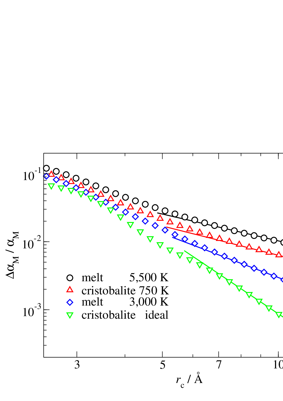
A surprising result of Fig. 6 is the relatively fast convergence of the Wolf summation for the “low-temperature” ($T=3,000$ K) melt, which is not only faster than at $T=5,500$ K melt but also faster than for the 750 K, thermal crystal. This may have to do with the fact that Madelung sums should actually converge for homoegeneous melts since the (partial) density autocorrelation function in dense liquids are damped oscillations at large $r$ not “suffering” from distant neighbor shells carrying large number of atoms and thereby preventing lattice sums from unconditional convergence. Ultimately, (twice) the electrostatic energy per point charge can be cast as an integral over the charge-density autocorrelation function, $C_{\rho\rho}(r)\equiv\langle\rho(0)\rho(r)\rangle$ via

where $0^{+}$ is meant to indicate that self-interactions of charges at $r=0$ are excluded from the integral. The (negative) integrand in the last term of Eq. (9) is shown in Fig. 7. It reveals that subsequent peaks in the integrand become ever smaller in the melt but not nexessarily in the crystal. In dense, three-dimensional liquid this behavior can be rationalized using the Ornstein-Zernike theory [31], which predicts density oscillations to obey asymptotically $\cos(r/\lambda+\varphi)\exp(-r/\zeta)$, where $\lambda$ is a wavelength, $\varphi$ a phase shift and $\zeta$ a correlation length. Maxima and minima in the negative integrand, which could be interpreted as a Madelung constant density, are located near the maxima of the partial dislike and like-ion radial distribution functions, respectively. While the magnitude of the integrand for large $r$ is clearly bound by a simple exponential in the liquid, this is not true for the crystal, where the extrema at $r\gtrsim 9$ Å and $r\lesssim 10$ Å are more pronounced than those in the interval $7$–$8$ Å.

As a small side remark to this article, we wish to note that the computational burden of the regular Ewald summation can be slightly reduced when the Fourier part of the interaction is not evaluated every time step but only every ${\cal{O}}(a_{0}k_{\textrm{E}})$ time steps. Such a reduction is possible, because the long-wavelength dynamics are slower than the ones associated with short wavelengths. The CPU time needed for the real-space sum would then scale as before with $Nr_{\textrm{c}}^{3}$, while the Fourier part would be reduced from $k_{\textrm{E}}^{3}N^{2}$ to $k_{\textrm{E}}^{4}N^{2}$, assuming that, say a wavenumber cutoff of $k_{\textrm{c}}\approx 4k_{\textrm{E}}$ is generally acceptable. For systems with stark (charge) heterogeneity on arbitrary wavelengths, it would be required to chose $k_{\textrm{c}}\propto 1/r_{\textrm{c}}$ as to avoid uncontrollable summation errors, which would otherwise arise if a structural heterogeneity existed on a wavelength exceeding simultaneously $r_{\textrm{c}}$ and $2\pi/k_{\textrm{c}}$. Minimizing the total CPU time through a proper choice of $k_{\textrm{E}}$ would then lead to a $N^{10/7}$ rather than a $N^{3/2}$ scaling of the numerical effort with particle number $N$.

References

- [1] M. P. Allen and D. J. Tildesley. Computer Simulation of Liquids. Oxford University Press, 2017.
- [2] D. Frenkel and B. Smit. Understanding Molecular Simulation. Elsevier, 2002.
- [3] F. H. Stillinger and T. A. Weber. Computer simulation of local order in condensed phases of silicon. Phys. Rev. B, 31(8):5262–5271, 1985.
- [4] J. Tersoff. New empirical model for the structural properties of silicon. Phys. Rev. Lett., 56(6):632–635, 1986.
- [5] P. J. Steinbach and B. R. Brooks. New spherical-cutoff methods for long-range forces in macromolecular simulation. J. Comp. Chem., 15(7):667–683, 1994.
- [6] M. Patra, M. Karttunen, M.T. Hyvönen, E. Falck, P. Lindqvist, and I. Vattulainen. Molecular dynamics simulations of lipid bilayers: Major artifacts due to truncating electrostatic interactions. Biophys. J., 84(6):3636–3645, 2003.
- [7] A. Mattoni, L. Colombo, and F. Cleri. Atomic scale origin of crack resistance in brittle fracture. Phys. Rev. Lett., 95(11), 2005.
- [8] L. Pastewka, P. Pou, R. Pérez, P. Gumbsch, and M. Moseler. Describing bond-breaking processes by reactive potentials: Importance of an environment-dependent interaction range. Phys. Rev. B, 78(16), 2008.
- [9] D. A. C. Beck, R. S. Armen, and V. Daggett. Cutoff size need not strongly influence molecular dynamics results for solvated polypeptides. Biochem., 44(2):609–616, JAN 18 2005.
- [10] C. Waibel, M. S. Feinler, and J. Gross. A modified shifted force approach to the Wolf summation. J. Chem. Theo. Comp., 15(1):572–583, 2019.
- [11] M. S. Daw and M. I. Baskes. Embedded-atom method: Derivation and application to impurities, surfaces, and other defects in metals. Phys. Rev. B, 29(12):6443–6453, 1984.
- [12] D. Wolf, P. Keblinski, S. R. Phillpot, and J. Eggebrecht. Exact method for the simulation of coulombic systems by spherically truncated, pairwise summation. J. Chem. Phys., 110(17):8254–8282, 1999.
- [13] C. J. Fennell and J. D. Gezelter. Is the Ewald summation still necessary? Pairwise alternatives to the accepted standard for long-range electrostatics. J. Chem. Phys., 124(23):234104, 2006.
- [14] H. M. Evjen. On the stability of certain heteropolar crystals. Phys. Rev., 39(4):675–687, 1932.
- [15] P. P. Ewald. Die Berechnung optischer und elektrostatischer Gitterpotentiale. Ann. Phys., 369(3):253–287, 1921.
- [16] U. Essmann, L. Perera, M. L. Berkowitz, T. Darden, H. Lee, and L. G. Pedersen. A smooth particle mesh Ewald method. J. Chem. Phys., 103(19):8577–8593, 1995.
- [17] M. Tuckerman, B. J. Berne, and G. J. Martyna. Reversible multiple time scale molecular dynamics. J. Chem. Phys., 97(3):1990–2001, 1992.
- [18] M. H. Müser, S. V. Sukhomlinov, and L. Pastewka. Interatomic potentials: Achievements and challenges, 2022.
- [19] M. I. Baskes, J. S. Nelson, and A. F. Wright. Semiempirical modified embedded-atom potentials for silicon and germanium. Phys. Rev. B, 40(9):6085–6100, 1989.
- [20] J. Jalkanen and M. H Müser. Systematic analysis and modification of embedded-atom potentials: case study of copper. Model. Simulat. Mater. Sci. Eng., 23(7):074001, 2015.
- [21] S. V. Sukhomlinov and M. H. Müser. Determination of accurate, mean bond lengths from radial distribution functions. J. Chem. Phys., 146(2):024506, 2017.
- [22] Pieter J. in ’t Veld, Ahmed E. Ismail, and Gary S. Grest. Application of Ewald summations to long-range dispersion forces. J. Chem. Phys., 127(14):144711, 2007.
- [23] S. W. de Leeuw, J. W. Perram, and E. R. Smith. Simulation of electrostatic systems in periodic boundary conditions. i. lattice sums and dielectric constants. Proc. R. Soc. A: Math. Phys. Eng. Sci., 373(1752):27–56, 1980.
- [24] J. W. Perram, H. G. Petersen, and S. W. De Leeuw. An algorithm for the simulation of condensed matter which grows as the 3/2 power of the number of particles. Mol. Phys., 65(4):875–893, 1988.
- [25] M. T. Dove, V. Heine, and K. D. Hammonds. Rigid unit modes in framework silicates. Mineral. Mag., 59(397):629–639, 1995.
- [26] M. H. Müser and K. Binder. Molecular dynamics study of the - transition in quartz: elastic properties, finite size effects, and hysteresis in the local structure. Phys. Chem. Min., 28(10):746–755, 2001.
- [27] B. W. H. van Beest, G. J. Kramer, and R. A. van Santen. Force fields for silicas and aluminophosphates based onab initiocalculations. Phys. Rev. Lett., 64(16):1955–1958, 1990.
- [28] K. Vollmayr, W. Kob, and K. Binder. Cooling-rate effects in amorphous silica: A computer-simulation study. Phys. Rev. B, 54(22):15808–15827, 1996.
- [29] D. Herzbach, K. Binder, and M. H. Müser. Comparison of model potentials for molecular-dynamics simulations of silica. J. Chem. Phys., 123(12):124711, 2005.
- [30] W. W. Schmahl, I. P. Swainson, M. T. Dove, and A. Graeme-Barber. Landau free energy and order parameter behaviour of the phase transition in cristobalite. Z. Kristallogr., 201(1-2):125–145, 1992.
- [31] R. J. Baxter. Ornstein–Zernike relation and Percus–Yevick approximation for fluid mixtures. J. Chem. Phys., 52(9):4559–4562, 1970.
- [32] G. A. Cisneros, M. Karttunen, P. Ren, and C. Sagui. Classical electrostatics for biomolecular simulations. Chem. Rev., 114(1):779–814, 2013.
- [33] N. Metropolis, A. W. Rosenbluth, M. N. Rosenbluth, A. H. Teller, and E. Teller. Equation of state calculations by fast computing machines. J. Chem. Phys., 21(6):1087–1092, 1953.