The Halo Bispectrum Multipoles in Redshift Space

Given the halo number density contrast $\delta_{h}(\mathbf{x})\equiv[n_{h}(\mathbf{x})-\bar{n}_{h}]/\bar{n}_{h}$ defined in terms of the number density $n_{h}(\mathbf{x})$ and its expectation value $\bar{n}=\langle n_{h}(\mathbf{x})\rangle$, and its Fourier transform¹¹ 1 We adopt the convention for the Fourier transform $$\delta(\mathbf{k})\equiv\int d^{3}x\,e^{-i\mathbf{k}\cdot\mathbf{x}}\,\delta(\mathbf{x})\,,$$ (2.1) with the inverse given by $$\delta(\mathbf{x})\equiv\int\frac{d^{3}k}{(2\pi)^{3}}\,e^{i\mathbf{k}\cdot\mathbf{x}}\,\delta(\mathbf{k})\,.$$ (2.2) $\delta_{h}(\mathbf{k})$ we can define the halo power spectrum $P_{h}$ and bispectrum $B_{h}$ respectively as

	$\displaystyle\langle\delta_{h}(\mathbf{k}_{1})\delta_{h}(\mathbf{k}_{2})\rangle$	$\displaystyle\equiv$	$\displaystyle(2\pi)^{3}\delta_{D}(\mathbf{k}_{12})\,P_{h}(k_{1})\,$		(2.3)
	$\displaystyle\langle\delta_{h}(\mathbf{k}_{1})\delta_{h}(\mathbf{k}_{2})\delta_{h}(\mathbf{k}_{3})\rangle$	$\displaystyle\equiv$	$\displaystyle(2\pi)^{3}\delta_{D}(\mathbf{k}_{123})\,B_{h}(k_{1},k_{2},k_{3})\,,$		(2.4)

where $\mathbf{k}_{12}=\mathbf{k}_{1}+\mathbf{k}_{2}$, $\mathbf{k}_{123}=\mathbf{k}_{1}+\mathbf{k}_{2}+\mathbf{k}_{3}$, and the Dirac deltas $\delta_{D}$ result from the assumed statistical homogeneity and isotropy. For the same reason $P_{h}(k_{1})$ is a function of one variable, $k_{1}=|\mathbf{k}_{1}|$ and $B_{h}(k_{1},k_{2},k_{3})$ is a function of the three sides of the triangle formed by $\mathbf{k}_{1}$, $\mathbf{k}_{2}$ and $\mathbf{k}_{3}$ and independent of its orientation.

In redshift-space, peculiar velocities $\mathbf{v}$ induce distortions in the galaxy distribution along the line-of-sight (LOS) $\hat{n}$. The observed position $\mathbf{s}$ will then be related to real position $\mathbf{x}$ by

$$\mathbf{s}=\mathbf{x}+\frac{\mathbf{v}\cdot\hat{n}}{a\,H(a)}\hat{n}\,.$$

(2.5)

As a result, clustering properties, and in particular galaxy correlation functions estimated in a given region of the sky, will depend on the local LOS. Since our focus is to test the modelling of the bispectrum based on measurements in simulation boxes with periodic boundary conditions, we will assume throughout this work the plane-parallel approximation for redshift-space distortions and therefore a global, constant LOS. The halo bispectrum will then be a function of the wavenumbers defining the triangular configuration $\mathbf{k}_{1}$, $\mathbf{k}_{2}$ and $\mathbf{k}_{3}$ plus the LOS $\hat{n}$, that is $B_{s}=B_{s}(\textbf{k}_{1},\textbf{k}_{2},\hat{n})$.

Our model for the redshift-space halo bispectrum is the sum of a deterministic and stochastic contribution, as

$$B_{s}(\mathbf{k}_{1},\mathbf{k}_{2},\mathbf{k}_{3})=B_{s}^{\rm(det)}(\mathbf{k}_{1},\mathbf{k}_{2},\mathbf{k}_{3})+B_{s}^{\rm(stoch)}(\mathbf{k}_{1},\mathbf{k}_{2},\mathbf{k}_{3})\,,$$

(2.6)

corresponding to the tree-level expression in Perturbation Theory (PT) resulting from the halo density given, in turn, by the sum of a deterministic and a stochastic component

$$\delta_{s}=\delta_{s}^{\rm(det)}+\delta_{s}^{\rm(stoch)}\,.$$

(2.7)

In Fourier space and up to the relevant order the deterministic contributions are given by

$$\delta_{s}^{\rm(det)}(\mathbf{k})=Z_{1}(\mathbf{k})\,\delta_{L}(\mathbf{k})+\int d^{3}q_{1}d^{3}q_{2}\delta_{D}(\mathbf{k}-\mathbf{q}_{12})Z_{2}(\mathbf{q}_{1},\mathbf{q}_{2})\,\delta_{L}(\mathbf{q}_{1})\,\delta_{L}(\mathbf{q}_{1})\,,$$

(2.8)

where $\delta_{L}$ is the linear matter overdensity and the redshift-space kernels are given in terms of the local ($b_{1}$, $b_{2}$) and tidal ($b_{\mathcal{G}_{2}}$) bias parameters and the linear growth rate $f$ by [39, 24, 26, 27, 40, 41, 42]

	$\displaystyle Z_{1}(\mathbf{k})$	$\displaystyle=$	$\displaystyle b_{1}+f\mu^{2}\,,$		(2.9)
	$\displaystyle Z_{2}(\mathbf{k}_{1},\mathbf{k}_{2})$	$\displaystyle=$	$\displaystyle\frac{b_{2}}{2}+b_{1}F_{2}(\mathbf{k}_{1},\mathbf{k}_{2})+b_{\mathcal{G}_{2}}S(\mathbf{k}_{1},\mathbf{k}_{2})+f\mu_{12}^{2}G_{2}(\mathbf{k}_{1},\mathbf{k}_{2})+$		(2.10)
			$\displaystyle+\frac{f\mu_{12}k_{12}}{2}\left[\frac{\mu_{1}}{k_{1}}Z_{1}(\textbf{k}_{2})+\frac{\mu_{2}}{k_{2}}Z_{1}(\textbf{k}_{1})\right]$

with $F_{2}$ and $G_{2}$ representing the usual matter density and velocity quadratic kernels and

$$S(\mathbf{k}_{1},\mathbf{k}_{2})=\left(\hat{k}_{1}\cdot\hat{k}_{2}\right)^{2}-1\,$$

(2.11)

while $\mu_{i}\equiv\mathbf{k}_{i}\cdot\hat{n}/k_{i}$ is the cosine of the angle formed by the wavenumber $\mathbf{k}_{i}$ with the LOS, specifically,

$$\mu_{12}=\frac{\mathbf{k}_{12}\cdot\hat{n}}{k_{12}}=-\frac{\textbf{k}_{3}\cdot\hat{n}}{k_{3}}=-\mu_{3}\,,$$

(2.12)

for a closed triangle with $\mathbf{k}_{123}=0$. The expansion of eq. (2.8) leads to the tree-level prediction for the bispectrum

$$B_{s}^{\rm(det)}(\mathbf{k}_{1},\mathbf{k}_{2},\hat{n})=2\,Z_{1}(\mathbf{k}_{1})\,Z_{1}(\mathbf{k}_{2})Z_{2}(\mathbf{k}_{1},\mathbf{k}_{2})P_{L}(k_{1})P_{L}(k_{2})+{\rm 2~perm.}\,$$

(2.13)

where $P_{L}(k)$ is the linear matter power spectrum.

The stochastic contribution to $\delta_{s}$ is given instead, following [42] and their notation, by

$$\delta_{s}^{\rm(stoch)}(\mathbf{x})=\epsilon(\mathbf{x})+\epsilon_{\delta}(\mathbf{x})\,\delta(\mathbf{x})+\epsilon_{\eta}(\mathbf{x})\eta(\mathbf{x})\,,$$

(2.14)

where $\epsilon$, $\epsilon_{\delta}$ and $\epsilon_{\eta}$ are stochastic fields uncorrelated to the density perturbations. The composite terms are limited to those linear in the matter density $\delta$ and in the l.o.s. derivative of the velocity component projected on the $\hat{n}$-axis $\eta\equiv\partial_{\hat{n}}(\mathbf{v}\cdot\hat{n})$, as these are responsible for the leading order contributions to the bispectrum. We neglect any higher-derivative operator in the stochastic contribution and we note that the last term should appear only due to selection effects [42]. In the large $k$ limit, we expect to recover the Poisson predictions for the power spectrum and bispectrum of the stochastic fields, that is [43]

	$\displaystyle\langle\epsilon(\mathbf{k}_{1})\epsilon(\mathbf{k}_{2})\rangle$	$\displaystyle\rightarrow\delta_{D}(\mathbf{k}_{12})\,\frac{1}{\bar{n}}\,,$		(2.15)
	$\displaystyle\langle\epsilon(\mathbf{k}_{1})\epsilon(\mathbf{k}_{2})\epsilon(\mathbf{k}_{3})\rangle$	$\displaystyle\rightarrow\delta_{D}(\mathbf{k}_{123})\,\frac{1}{\bar{n}^{2}}\,,$		(2.16)
	$\displaystyle\langle\epsilon(\mathbf{k}_{1})\epsilon_{\delta}(\mathbf{k}_{2})\rangle$	$\displaystyle\rightarrow\delta_{D}(\mathbf{k}_{123})\,\frac{b_{1}}{2\bar{n}}\,,$		(2.17)
	$\displaystyle\langle\epsilon(\mathbf{k}_{1})\epsilon_{\eta}(\mathbf{k}_{2})\rangle$	$\displaystyle\rightarrow\delta_{D}(\mathbf{k}_{123})\,\frac{1}{2\bar{n}}\,,$		(2.18)

where the first term only appears in the halo power spectrum, while the last three all contribute to the halo bispectrum. In principle we can expect independent departures from the Poisson prediction for all three terms, which in the large-scale limit can be described in terms of three constant parameters²² 2 In [23] the authors follow [44] in the modelling of the stochastic contribution assuming $$\delta_{s}^{(stoch)}=d_{1}\,\epsilon_{P}+d_{2}\,b_{1}\,\epsilon_{P}\,\delta+d_{1}\,\epsilon_{P}\,\eta\,,$$ (2.19) where the coefficients $d_{1}$ and $d_{2}$ parameterize the corrections to the Poisson prediction represented by field $\epsilon_{P}$ (for which the limits (2.15) and (2.16) hold as equalities). The Poisson case is recovered for $d_{1}=2\,d_{2}=1$. This implies that $\langle\epsilon\epsilon\rangle=\langle\epsilon\epsilon_{\eta}\rangle$ and their corrections to Poisson are therefore described by a single degree of freedom. They also relate $\langle\epsilon\epsilon\rangle$ and $\langle\epsilon\epsilon\epsilon\rangle$ but it does not seem justified. Such relation also appears inconsistent with the expansion above and it does not seem to be supported by the halo model description of [45]..

The corresponding stochastic contribution to the bispectrum at tree-level will then read

$\displaystyle B_{s}^{\rm(stoch)}(\mathbf{k}_{1},\mathbf{k}_{2},\hat{n})=\frac{1}{\bar{n}}\left[(1+\alpha_{1})\,b_{1}+(1+\alpha_{3})\,f\,\mu^{2}\right]\,Z_{1}(\mathbf{k}_{1})\,P_{L}(k_{1})+2~{\rm perm.}+\frac{1+\alpha_{2}}{\bar{n}^{2}}\,,$

(2.20)

where the parameters $\alpha_{i}$ vanish in the Poisson limit³³ 3 The notation for the $\alpha_{i}$ parameters is chosen in order to be consistent with 36 and 38, where $\alpha_{2}$ already appeared as correction to the $1/\bar{n}^{2}$ term, while $\alpha_{3}$ was not present..

In this work we do not consider any modelling of Finger-of-God effects as we expect them to be negligible at large scales and for a halo distribution.

We adopt the definition of the redshift-space multipoles of the bispectrum introduced by [27] (and assumed as well by [46] and [16]) where the vector configurations covering the domain of $B_{s}(\mathbf{k}_{1}\mathbf{k}_{2},\hat{n})$ are given in terms of the variables $k_{1}$, $k_{2}$, $k_{3}$, $\mu_{1}\equiv\cos(\theta)$ and $\xi$, with $\theta_{1}$ being the angle between $\mathbf{k}_{1}$ and the LOS while $\xi$ is the azimuthal angle describing a rotation of $\mathbf{k}_{2}$ around $\mathbf{k}_{1}$.

$B_{s}$ is then expanded in spherical harmonics as

$$B_{s}(k_{1},k_{2},k_{3},\theta,\xi)=\sum_{\ell}\sum_{m=-\ell}^{\ell}B_{\ell m}(k_{1},k_{2},k_{3})\,Y_{\ell}^{m}(\theta,\xi)$$

(2.21)

with the coefficients of the expansion given by

$$B_{\ell m}(k_{1},k_{2},k_{3})=\int_{-1}^{+1}\!\!d\!\cos{\theta}\int_{0}^{2\pi}d\xi B_{s}(k_{1},k_{2},k_{3},\theta,\xi)\,Y_{\ell}^{m}(\theta,\xi)\,.$$

(2.22)

We only consider $m=0$, even multipoles as the loss of information coming from excluding the $m\neq 0$ terms is negligible [16, 47]. In this case the spherical harmonics reduce to Legendre polynomials $\mathcal{L}_{\ell}$ and only depend on $\mu_{1}\equiv\cos\theta$,

$$Y_{\ell}^{0}(\theta,\xi)=\sqrt{\frac{2\ell+1}{4\pi}}\mathcal{L}_{\ell}(\mu_{1})\,$$

(2.23)

and the expansion of eq. (2.21) is replaced by

$$\frac{1}{2\pi}\int d\xi B_{s}(k_{1},k_{2},k_{3},\theta,\xi)=\sum_{\ell}\,B_{\ell}(k_{1},k_{2},k_{3})\,{\mathcal{L}}_{\ell}(\mu_{1})$$

(2.24)

where

	$\displaystyle B_{\ell}(k_{1},k_{2},k_{3})$	$\displaystyle=\sqrt{\frac{2\ell+1}{4\pi}}\,B_{\ell 0}(k_{1},k_{2},k_{3})$
		$\displaystyle=(2\ell+1)\frac{1}{2}\int_{-1}^{+1}\!\!d\!\cos{\theta}\Big[\frac{1}{2\pi}\int_{0}^{2\pi}d\xi B_{s}(k_{1},k_{2},k_{3},\theta,\xi)\Big]\,{\mathcal{L}}_{\ell}(\cos\theta)\,.$		(2.25)

The analysis is performed on redshift-space, halo bispectrum measurements from the set of 298 Minerva N-body simulations [48] whose real-space counterpart was already studied in 36 and 38. These follow the evolution of $1000^{3}$ dark matter particles in a cubic box of side $L=1500\,h^{-1}\,{\rm Mpc}$ and correspond to a total volume of about $1,000\,h^{-3}\,{\rm Gpc}^{3}$. Each halo catalog is defined by a minimal mass of $M\simeq 1.12\times 10^{13}\;h^{-1}M_{\odot}$. We refer the reader to 36 for a more detailed description of the simulations and of the halo catalog construction.

38 provides us with an estimate of the bias parameters characterising the halo population obtained as posteriors from the joint analysis of the halo power spectrum and bispectrum in real space. We will use these here as a reference for our redshift-space analysis, in addition to the value for the linear growth rate expected from the fiducial cosmology.

Our estimator of the bispectrum multipoles follow the definition of [27] for the $m=0$ case and constitutes an implementation of the one described in [46] based on Fast-Fourier Transforms. In our case, however, we assume a constant line-of-sight $\hat{n}$, corresponding to an exact realisation of the plane-parallel or distant observer approximation. The estimator reduces therefore to the following expression

$$\hat{B}_{\ell}=(2\ell+1)\frac{k_{f}^{3}}{N_{B}}\sum_{\mathbf{q}_{1}\in k_{1}}\sum_{\mathbf{q}_{2}\in k_{2}}\sum_{\mathbf{q}_{3}\in k_{3}}\,\delta_{K}(\mathbf{q}_{123})\,\delta_{s}(\mathbf{q}_{1})\,\delta_{s}(\mathbf{q}_{2})\,\delta_{s}(\mathbf{q}_{3})\,\mathcal{L}_{\ell}(\hat{q}_{1}\cdot\hat{n})\,,$$

(3.1)

where the sums, accounting for the discrete nature of the Fourier Transform $\delta_{s}(\mathbf{q})$ of the halo density in a simulation box, are over all wavenumbers $\mathbf{q}_{i}$ falling into the bin centered at $k_{i}$ of radial size $\Delta k$, that is, such that $k_{i}-\Delta k/2\leq|\mathbf{q}_{i}|<k_{i}+\Delta k/2$. Also, $\delta_{K}(\mathbf{q})$ is a Kronecker symbol equal to unity for $\mathbf{q}={\bf 0}$ and vanishing otherwise, while the normalisation factor

$$N_{B}(k_{1},k_{2},k_{3})=\sum_{\mathbf{q}_{1}\in k_{1}}\sum_{\mathbf{q}_{2}\in k_{2}}\sum_{\mathbf{q}_{3}\in k_{3}}\,\delta_{K}(\mathbf{q}_{123})\,,$$

(3.2)

provides the number of “fundamental triangles” $\{\mathbf{q}_{1},\mathbf{q}_{2},\mathbf{q}_{3}\}$ present in the “triangle bin” $\{k_{1},k_{2},k_{3}\}$. The grid-interpolation of the halo density $\delta_{s}(\mathbf{q})$ is obtained by means of a fourth-order mass assignment scheme and adopts the interlacing technique for aliasing reduction [49]. All bispectrum measurements, unless otherwise stated, assume a wavenumber bin size $\Delta k=k_{f}$, that is corresponding to the fundamental frequency characterising the simulation box, $k_{f}\equiv 2\pi/L$. This leads to the measurement of 1475 triangular configurations up to $k_{\rm max}=0.1\,h\,{\rm Mpc}^{-1}$ for each multipole⁴⁴ 4 We include “open triangle bins”, that is those where the bin centers cannot form a closed triangle such as $\{k_{1},k_{2},k_{3}\}=\{6,3,2\}k_{f}$ but that nevertheless contain closed fundamental triplets $\{\mathbf{q}_{1},\mathbf{q}_{2},\mathbf{q}_{3}\}$. See section 2.2 of 36 for a detailed description of the binning definition..

Figure 1 shows the mean of the bispectrum multipoles measured from the 298 Minerva N-body simulations for all triangular configurations. In these type of plots, the ordering of the configurations is determined by increasing values of $k_{1}$, $k_{2}$, $k_{3}$ which obey the requirement, $k_{1}\geq k_{2}\geq k_{3}$ (see 36 for a more detailed explanation). Vertical gray lines mark the triangle where the value of $k_{1}$ changes, so that all configurations on the left correspond to triangles made up with sides smaller or equal to such value of $k_{1}$. All measurements include shot-noise. The bottom half of each panel shows the relative error on the mean, along with the ratio between the expected Poisson shot-noise contribution and the overall signal (black, dashed lines).

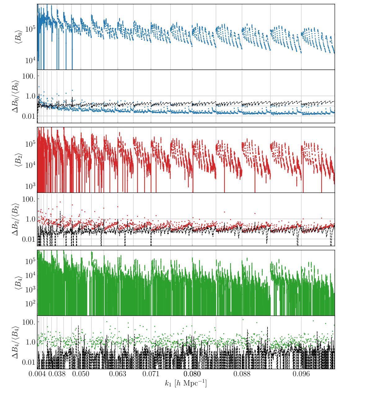
We notice that the relative error on the mean for the bispectrum monopole is at the ten-percent level and just slightly smaller at smaller scales. The shot-noise level is comparable to the statistical error at large scales and it is larger at smaller scales, as it happens in real-space for this halo population (see 36). The relative error on the quadrupole and hexadecapole mean is instead of the order of tens of percent and hundreds of percent, respectively. Because of the first term on the r.h.s. of (2.20), all multipoles receive a shot-noise contribution. This is comparable to the error on the mean for the quadrupole and lower by an order of magnitude for the hexadecapole.

As for 36 and 38, the covariance properties of our observables are estimated from a much larger set of 10,000 measurements from mock halo catalogs obtained with the Pinocchio code [50, 51, 52]. The mocks share the same cosmology, box size and resolution with the Minerva simulations and 298 realisations also adopt the same initial conditions. The mass threshold for the mocks is chosen to reproduce (below percent level) the amplitude of the large-scale halo power spectrum (including shot-noise) of the numerical simulations (see 36 for details). This quantity, in fact, determines the Gaussian contribution to the bispectrum covariance, the leading one for most triangular configurations (see also [53, 54]).

The covariance matrix for each bispectrum multipole and their cross-covariance is defined as

$$C_{\ell_{1}\ell_{2}}(t_{i},t_{j})\equiv\langle\hat{B}_{\ell_{1}}(t_{i})\,\hat{B}_{\ell_{2}}(t_{j})\rangle-\langle\hat{B}_{\ell_{1}}(t_{i})\rangle\langle\hat{B}_{\ell_{2}}(t_{j})\rangle\,,$$

(4.1)

where $t_{i}=\{k_{1i},k_{2i},k_{3i}\}$ and $t_{j}=\{k_{1j},k_{2j},k_{3j}\}$ represent two triangle configurations. We will denote as $\hat{C}_{\ell_{1}\ell_{2}}(t_{i},t_{j})$ its estimate from the 10,000 mock catalogs.

The left column of figure 2 shows the ratio between the mean of each bispectrum multipole measured in the numerical simulations and the mean of the same quantity measured in the Pinocchio mocks, limited to the 298 mocks with matching initial conditions. We find for the monopole the same discrepancy, as large as 7-8% depending on the triangle shape, already encountered in real space (see 36). The noise in the measurements for the higher-order multipoles, on the other hand, does not allow to clearly identify systematic differences at the level of 10% or below. The right column of figure 2 shows instead the ratio between the variance $\Delta B_{\ell}(t_{i})\equiv C_{\ell\ell}(t_{i},t_{i})$, estimated again from the numerical simulations and the one estimated from the Pinocchio mocks. Again, the Pinocchio set is limited here to the 298 realisations with matching seeds. Despite possible systematics on the observables, the variance is recovered by the Pinocchio mocks with an error below 10% and no apparent systematic difference for all multipoles. This is expected, given the close match of the power spectra and the fact that the leading contribution to the bispectrum covariance is fully determined by the power spectrum, see Eq. (4.2).

In addition to the numerical estimate of the covariance we consider as well the analytical prediction in the Gaussian approximation. The Gaussian contribution enters the variance of each multipole, $\Delta B_{\ell}\equiv C_{\ell\ell}(t_{i},t_{i})$, but also the correlation $C_{\ell_{1}\ell_{2}}(t_{i},t_{i})$ between $\hat{B}_{\ell_{1}}(t_{i})$ and $\hat{B}_{\ell_{2}}(t_{i})$ with $\ell_{1}\neq\ell_{2}$ but measured for the same triangle $t_{i}$.

From the definition of the multipoles estimators, eq. (3.1), we can write

	$\displaystyle C_{\ell_{1}\ell_{2}}(k_{1},k_{2},k_{3})$	$\displaystyle\equiv\langle\hat{B}_{\ell_{1}}\hat{B}_{\ell_{2}}\rangle-\langle\hat{B}_{\ell_{1}}\rangle\langle\hat{B}_{\ell_{2}}\rangle$
		$\displaystyle=(2\ell_{1}+1)(2\ell_{2}+1)\frac{k_{f}^{6}}{N^{2}_{B}}\sum_{\mathbf{q}_{1}\in k_{1}}\sum_{\mathbf{q}_{2}\in k_{2}}\sum_{\mathbf{q}_{3}\in k_{3}}\,\delta_{K}(\mathbf{q}_{123})\,\sum_{\mathbf{p}_{1}\in k_{1}}\sum_{\mathbf{p}_{2}\in k_{2}}\sum_{\mathbf{p}_{3}\in k_{3}}\,\delta_{K}(\mathbf{p}_{123})$
		$\displaystyle\times\,\mathcal{L}_{\ell_{1}}(\mu_{\mathbf{q}_{1}})\,\mathcal{L}_{\ell_{2}}(\mu_{\mathbf{p}_{1}})\,\Big[\langle\delta_{\mathbf{q}_{1}}\,\delta_{\mathbf{q}_{2}}\,\delta_{\mathbf{q}_{3}}\delta_{\mathbf{p}_{1}}\,\delta_{\mathbf{p}_{2}}\,\delta_{\mathbf{p}_{3}}\rangle-\langle\delta_{\mathbf{q}_{1}}\,\delta_{\mathbf{q}_{2}}\,\delta_{\mathbf{q}_{3}}\rangle\langle\delta_{\mathbf{p}_{1}}\,\delta_{\mathbf{p}_{2}}\,\delta_{\mathbf{p}_{3}}\rangle\Big]\,.$		(4.2)

In the Gaussian approximation, from the expectation values on the r.h.s. of the equation above, we retain only the contributions depending on the power spectrum. Assuming (without loss of generality) that $k_{1}\geq k_{2}\geq k_{3}$, these are given by

	$\displaystyle C_{\ell_{1}\ell_{2}}^{G}(k_{1},k_{2},k_{3})$	$\displaystyle=\frac{(2\ell_{1}+1)(2\ell_{2}+1)}{N^{2}_{B}\,k_{f}^{3}}\sum_{\mathbf{q}_{1}\in k_{1}}\sum_{\mathbf{q}_{2}\in k_{2}}\sum_{\mathbf{q}_{3}\in k_{3}}\,\delta_{K}(\mathbf{q}_{123})\,P_{tot}(\mathbf{q}_{1})\,P_{tot}(\mathbf{q}_{2})\,P_{tot}(\mathbf{q}_{3})$
		$\displaystyle\times\Big[(1+\delta^{K}_{k_{2},k_{3}})\,\mathcal{L}_{\ell_{1}}(\mu_{\mathbf{q}_{1}})\mathcal{L}_{\ell_{2}}(-\mu_{\mathbf{q}_{1}})+(\delta^{K}_{k_{1},k_{2}}+\delta^{K}_{k_{2},k_{3}})\,\mathcal{L}_{\ell_{1}}(\mu_{\mathbf{q}_{1}})\mathcal{L}_{\ell_{2}}(-\mu_{\mathbf{q}_{2}})+$
		$\displaystyle+2\,\delta^{K}_{k_{1},k_{3}}\,\mathcal{L}_{\ell_{1}}(\mu_{\mathbf{q}_{1}})\mathcal{L}_{\ell_{2}}(-\mu_{\mathbf{q}_{3}})\Big]\,,$		(4.3)

where $P_{tot}(\mathbf{q}_{1})=P(\mathbf{q}_{1})+P_{SN}$ is the anisotropic halo power spectrum including a shot-noise contribution while $\delta^{K}_{k_{i},k_{j}}$ is the Kronecker symbol equal to one for $k_{i}=k_{j}$, and vanishing otherwise. Notice that the terms in the square brackets correspond, in the case $\ell_{1}=\ell_{2}=0$, to the usual factor equal to 6, 2 and 1 respectively for equilateral, isosceles and scalene triangles.

Similarly to the power spectrum variance case, see e.g. [48], we can expand the anisotropic power spectra in multipoles to obtain

	$\displaystyle C_{\ell_{1}\ell_{2}}^{G}$	$\displaystyle=\frac{(2\ell_{1}+1)(2\ell_{2}+1)}{N^{2}_{B}\,k_{f}^{3}}\sum_{\ell_{3},\ell_{4},\ell_{5}}\sum_{\mathbf{q}_{1}\in k_{1}}\sum_{\mathbf{q}_{2}\in k_{2}}\sum_{\mathbf{q}_{3}\in k_{3}}\,\delta_{K}(\mathbf{q}_{123})\,P_{tot,\,\ell_{3}}(q_{1})\,P_{tot,\,\ell_{4}}(q_{2})\,P_{tot,\,\ell_{5}}(q_{3})$
		$\displaystyle\times\Big[(1+\delta^{K}_{k_{2},k_{3}})\,\mathcal{L}_{\ell_{1}}(\mu_{\mathbf{q}_{1}})\mathcal{L}_{\ell_{2}}(-\mu_{\mathbf{q}_{1}})+(\delta^{K}_{k_{1},k_{2}}+\delta^{K}_{k_{2},k_{3}})\,\mathcal{L}_{\ell_{1}}(\mu_{\mathbf{q}_{1}})\mathcal{L}_{\ell_{2}}(-\mu_{\mathbf{q}_{2}})+$
		$\displaystyle+2\,\delta^{K}_{k_{1},k_{3}}\,\mathcal{L}_{\ell_{1}}(\mu_{\mathbf{q}_{1}})\mathcal{L}_{\ell_{2}}(-\mu_{\mathbf{q}_{3}})\Big]\mathcal{L}_{\ell_{3}}(\mu_{1})\mathcal{L}_{\ell_{4}}(\mu_{2})\mathcal{L}_{\ell_{5}}(\mu_{3})\,.$		(4.4)

This is the expression we adopt in our evaluation of the Gaussian variance, with the sums over the $k$-shells performed exactly over the discrete wavenumbers $\mathbf{q}$ defining the Fourier-space density grid⁵⁵ 5 It is possible to simplify further this expression in the thin-shell approximation so that $\displaystyle C_{\ell_{1}\ell_{2}}^{G}$ $\displaystyle\simeq\frac{(2\ell_{1}+1)(2\ell_{2}+1)}{N_{B}\,k_{f}^{3}}\sum_{\ell_{3},\ell_{4},\ell_{5}}P_{tot,\,\ell_{3}}(k_{1})\,P_{tot,\,\ell_{4}}(k_{2})\,P_{tot,\,\ell_{5}}(k_{3})R_{\ell_{1},\ell_{2};\ell_{3}\ell_{4},\ell_{5}}(k_{1},k_{2},k_{3})\,.$ (4.5) where we defined $\displaystyle R_{\ell_{1},\ell_{2};\ell_{3}\ell_{4},\ell_{5}}(k_{1},k_{2},k_{3})$ $\displaystyle\equiv\frac{1}{N_{B}}\sum_{\mathbf{q}_{1}\in k_{1}}\sum_{\mathbf{q}_{2}\in k_{2}}\sum_{\mathbf{q}_{3}\in k_{3}}\,\delta_{K}(\mathbf{q}_{123})\,$ $\displaystyle\times\Big[(1+\delta^{K}_{k_{2},k_{3}})\,\mathcal{L}_{\ell_{1}}(\mu_{\mathbf{q}_{1}})\mathcal{L}_{\ell_{2}}(-\mu_{\mathbf{q}_{1}})+(\delta^{K}_{k_{1},k_{2}}+\delta^{K}_{k_{2},k_{3}})\,\mathcal{L}_{\ell_{1}}(\mu_{\mathbf{q}_{1}})\mathcal{L}_{\ell_{2}}(-\mu_{\mathbf{q}_{2}})+$ $\displaystyle+2\,\delta^{K}_{k_{1},k_{3}}\,\mathcal{L}_{\ell_{1}}(\mu_{\mathbf{q}_{1}})\mathcal{L}_{\ell_{2}}(-\mu_{\mathbf{q}_{3}})\Big]\mathcal{L}_{\ell_{3}}(\mu_{1})\mathcal{L}_{\ell_{4}}(\mu_{2})\mathcal{L}_{\ell_{5}}(\mu_{3})\,.$ (4.6) In the continuum limit, we can replace the sums over the shells with integrals and reduced them to a simple average over the orientation of the triangle $\left\{\mathbf{q}_{1},\mathbf{q}_{2},\mathbf{q}_{3}\right\}$, that is $$\frac{1}{N_{B}}\sum_{\mathbf{q}_{1}\in k_{1}}\sum_{\mathbf{q}_{2}\in k_{2}}\sum_{\mathbf{q}_{3}\in k_{3}}\,\delta_{K}(\mathbf{q}_{123})\simeq\frac{1}{N_{B}\,k_{f}^{6}}\prod_{i=1}^{3}\int_{k_{i}}d^{3}q_{i}\,\delta_{D}(\mathbf{q}_{123})=\frac{1}{4\pi}\int_{-1}^{1}d\mu_{1}\!\!\int d\xi\,,$$ (4.7) with an integrand that is now only a function of powers of $\mu_{1}$, $\mu_{2}$ and $\mu_{3}$. Then, assumming only even values for $\ell_{3}$, $\ell_{4}$ and $\ell_{5}$ (and clearly for $\ell_{1}$ and $\ell_{2}$), we can use the expansion for the Legendre polynomials $$\mathcal{L}(\mu)=\frac{1}{2^{\ell}}\sum_{n=1}^{\ell/2}\frac{(-1)^{n}(2\ell-2n)!}{n!(\ell-n)!(\ell-2n)!}\mu^{\ell-2n}\equiv\sum_{n=1}^{\ell/2}C_{\ell,n}\mu^{\ell-2n}$$ (4.8) to get an expression that can be automatically evaluated with a software allowing for symbolic manipulation, $\displaystyle R_{\ell_{1},\ell_{2};\ell_{3}\ell_{4},\ell_{5}}(k_{1},k_{2},k_{3})$ $\displaystyle\simeq\prod_{i=1}^{5}\sum_{n_{i}=1}^{\ell_{i}/2}C_{\ell_{i},n_{i}}\Big[(1+\delta^{K}_{k_{2},k_{3}})\mathcal{I}_{\ell_{1}+\ell_{2}+\ell_{3}-2(n_{1}+n_{2}+n_{3}),\,\ell_{4}-2n_{4},\,\ell_{5}-2n_{5}}$ $\displaystyle+(\delta^{K}_{k_{1},k_{2}}+\delta^{K}_{k_{2},k_{3}})\mathcal{I}_{\ell_{1}+\ell_{3}-2(n_{1}+n_{3}),\,\ell_{2}+\ell_{4}-2(n_{2}+n_{4}),\,\ell_{5}-2n_{5}}$ $\displaystyle+2\,\delta^{K}_{k_{1},k_{3}}\,\mathcal{I}_{\ell_{1}+\ell_{3}-2(n_{1}+n_{3}),\,\ell_{4}-2n_{4},\,\ell_{2}+\ell_{5}-2(n_{2}+n_{5})}\Big]\,,$ (4.9) , where the integrals $\mathcal{I}_{\alpha,\beta,\gamma}$ are defined in Appendix A. .

The comparison between the numerical estimate and analytic prediction for these quantities is shown in figure 3. One can see how the Gaussian prediction for $C_{00}$, $C_{22}$ and $C_{44}$ is able to describe the measured ones at the level of 5%, with a slight deficit noticeable in the monopole and quadrupole case for squeezed triangles, due to the missing non-Gaussian contribution [53, 54]. The agreement in the case of the cross-covariance $C_{\ell_{1}\ell_{2}}(t_{i},t_{i})$ is also rather good, with the theory underestimating the measurements by an overall 10%. In these cases the ratio can take large values when the denominator is close to zero, as it is the case particularly for $C_{0,4}$.

Finally, figure 4 shows a subset of the correlation matrix, defined as

$$r_{\ell_{1}\ell_{2}}(t_{i},t_{j})=\frac{C_{\ell_{1}\ell_{2}}(t_{i},t_{j})}{\sqrt{C_{\ell_{1}\ell_{1}}(t_{i},t_{i})\,C_{\ell_{2}\ell_{2}}(t_{j},t_{j})}}\,.$$

(4.10)

Each data-set $\hat{B}_{\ell}(t_{i})$ is restricted, for illustration purposes, to its first 32 triangular configurations $t_{i}$, denoted in the figure in terms of the three sides in units of the fundamental frequency, that is $\{k_{1},k_{2},k_{3}\}/k_{f}$. It follows that while the block-diagonal matrices show the correlation coefficients $r_{\ell\ell}(t_{i},t_{j})$ for each multipoles, the off-diagonal matrices depict their relative cross-covariance $r_{\ell_{1}\ell_{2}}(t_{i},t_{j})$. In addition, the top-right half is estimated from the full set of 10,000 Pinocchio mocks, while the bottom-left half is the theoretical prediction in the Gaussian approximation, vanishing for all elements with $t_{i}\neq t_{j}$. The bottom panels compare in more detail the predicted and measured coefficients $r_{\ell_{1}\ell_{2}}(t_{i},t_{i})$ with $\ell_{1}\neq\ell_{2}$ as a function of the selected triangles $t_{i}$. On these quantities the agreement between theory and numerical estimates is truly remarkable and extends up to $k_{\rm max}\sim 0.1\,h\,{\rm Mpc}^{-1}$, that is over the full range of scales that we will consider in the analysis described in the following sections.

Regarding the structure of the correlation coefficient, it is clear that only the elements corresponding to the expected Gaussian contributions appear to be relevant at these large scales. These, however, are not limited to the diagonal for the full data vector $D=\left\{B_{0},B_{2},B_{4}\right\}$, but obviously include all elements corresponding to the correlation between different multipoles sharing the same triangles.

Following 36 and 38, we fit all measurements together assuming their independence. This means that our total log-likelihood function corresponds to the sum of the log-likelihood for each individual realisation,

$$\ln{\mathcal{L}}_{\rm tot}=\sum_{\alpha=1}^{N_{R}}\ln{\mathcal{L}}_{\rm\alpha}\,,$$

(5.1)

where $N_{R}$ is the total number of realisations considered.

We work under the assumption of Gaussianity for the individual likelihood ${\mathcal{L}}_{\rm\alpha}$. However, we follow [55] in order to account for possible uncertainties in the determination of the precision matrix due to a limited number of mocks. The log-likelihood for a single realisation is then, modulo an additive, normalization constant,

$$\ln{\mathcal{L}}_{\alpha}=-\frac{N_{M}}{2}\ln\Big[1+\frac{\chi^{2}_{\alpha}}{N_{M}-1}\Big]\,,$$

(5.2)

where $N_{M}$ is the number of mock catalogs used for the numerical estimation of the covariance matrix (we refer the reader to 36 for further details). In this expression $\chi_{\alpha}^{2}$ represents the chi-square statistic for the individual realisation, given by

$$\chi^{2}_{\alpha}=\sum_{i,j=1}^{N_{D}}\left[\hat{D}^{(\alpha)}_{i}-D^{(theory)}_{i}\right]C_{ij}^{-1}\left[\hat{D}^{(\alpha)}_{j}-D^{(theory)}_{j}\right]\,,$$

(5.3)

where, in the most general case, $\hat{D}^{(\alpha)}\equiv\left\{\hat{B}_{0},\hat{B}_{2},\hat{B}_{4}\right\}$ is the data vector, of size $N_{D}$, encompassing the three bispectrum multipoles while $D^{(theory)}$ and $C_{ij}$ are, respectively, the corresponding theoretical model and covariance matrix.

We should notice that given the large number of 10,000 Pinocchio realisations, even for the largest data-set corresponding to the joint analysis of the three bispectrum multipoles up to $k_{\rm max,B}=0.1\,h\,{\rm Mpc}^{-1}$, with a total of $1,475\times 3\simeq 4,425$ data-points, the difference w.r.t. the Gaussian case is in fact negligible. The alternative approach of re-scaling the inverse covariance, as suggested in [56, 57], gives rise to error bars up to 10% larger, although we have checked that these do not lead to any appreciable differences in the recovered parameter posteriors that we discuss below.

Our main goal is assessing the validity and reach of the tree-level bispectrum model, eqs. (2.13) and (2.20) leaving the exploration of their potential to constrain cosmological parameters to a future work. For this reason, in our Bayesian analyses we assume galaxy bias, shot-noise and the growth rate $f$ as the only free parameters. The bispectrum multipoles defined in eq. (2.22) can be written as a linear combination of several contributions where the dependence on these parameters can be factorised, leading to a quick exploration of the likelihood function since each term only needs to be computed once for the fiducial cosmology.

This allows as well for an exact binning of the theoretical model, taking advantage of the discrete Fourier-space grid characterising numerical simulations in boxes with periodic boundary conditions. In this case we can sum $B_{s}(\mathbf{q}_{1},\mathbf{q}_{2},\mathbf{q}_{3},\hat{n})$ over all discrete modes $\mathbf{q}_{i}$ forming a close triangle $\mathbf{q}_{123}=0$ and belonging to the bin $\{k_{1},k_{2},k_{3}\}$. This leads to

$$B_{\ell}^{\rm(binned)}(k_{1},k_{2},k_{3})=\frac{2\ell+1}{N_{B}}\sum_{\mathbf{q}_{1}\in k_{1}}\sum_{\mathbf{q}_{2}\in k_{2}}\sum_{\mathbf{q}_{3}\in k_{3}}\delta_{K}(\mathbf{q}_{123})B_{s}(\mathbf{q}_{1},\mathbf{q}_{2},\mathbf{q}_{3},\hat{n})\mathcal{L}_{\ell}(\hat{q}_{1}\cdot\hat{n}),$$

(5.4)

where the sums account for the angle-average defining the bispectrum multipoles.

This approach requires the evaluation of the bispectrum model over a very large number of triangular configurations, making it unfeasible in a Bayesian analysis where cosmological parameters are explored. An approximate solution would be to evaluate the model $B_{\ell}$ on a single triangle defined by effective values of the wavenumbers. This approach, that takes advantage of the analytical evaluation of the angle integrals in (2.2) described in Appendix A, is presented in Appendix 6.6 along with a quantification of the systematic errors resulting in the parameters determination.

We will assess the goodness of the fits that we will perform in terms of the posterior predictive $p$-value (ppp) and the posterior-averaged reduced chi-square $\langle\chi^{2}_{\nu}\rangle_{\rm post}$. The ${\rm ppp}$ assumes values between 0 and 1, and we use the treshold ${\rm ppp}\geq 0.95$ to reject the model. The $\langle\chi^{2}_{\nu}\rangle_{\rm post}$ is compared to the 95 percent (upper) confidence limit associated to a number of degrees of freedom equal to the total number of data points fitted: when $\langle\chi^{2}_{\nu}\rangle_{\rm post}$ is greater than this value, the model fails to describe the data. For the comparison between different models and assumptions on the bias parameters, we use the Deviance Information Criterion (DIC) computed from the MCMC simulations. For details on the choice of these diagnostics, we redirect the reader to 36.

We start with a test of the full model in which all seven bias and shot-noise parameters are free to vary. We compare the fit to the bispectrum monopole to the joint analysis of monopole and higher-order multipoles, assuming the full volume of the 298 Minerva simulations. The first goal is to identify the set of parameters that can effectively be determined by our data-set, and the relative importance of the different multipoles in setting their constraints. We assume uniform priors on all parameters, with bounds specified in table 1.

The main results are shown in figure 5. The left panels show the marginalised, 68.3% credibility regions for the model parameters as a function of the maximum wavenumber included in the triangle selection. Two-dimensional marginalised contours are shown in the bottom-right panel for the $k_{\rm max}=0.06\,h\,{\rm Mpc}^{-1}$ case (indicated as the vertical, dotted line in the other two sub-panels). Finally, the top-right panel shows the posterior-averaged, reduced chi-square, $\langle\chi_{\nu}^{2}\rangle$ and the posterior predictive $p$-value.

The tree-level model described in section 2.1 provides a good fit to the data up to a $k_{\rm max}\simeq 0.08\,h\,{\rm Mpc}^{-1}$ for the monopole, while the reach is restricted to 0.06 and 0.045$\,h\,{\rm Mpc}^{-1}$, respectively, when $B_{2}$ and $B_{4}$ are also considered.

For $k_{\rm max}=0.06\,h\,{\rm Mpc}^{-1}$, the combination $B_{0}+B_{2}$ properly recovers the best-fit values of the bias parameters obtained from the joint analysis of the real-space power spectrum and bispectrum along with the fiducial value of the linear growth rate $f$, which are shown by the gray, dashed lines in the bottom-right panel.

The addition of the quadrupole $B_{2}$ greatly reduces the large degeneracy between the linear bias $b_{1}$ and the growth rate $f$, as well as with the quadratic bias parameters, characterising the monopole-only constraints. This qualitatively confirms the expectation that the bispectrum monopole does not fully capture the information potentially present in the anisotropic, redshift-space bispectrum [17, 58]. On the other hand, including as well the hexadecapole leads to no significant improvement for any parameter and we will drop it for all the tests that will follow.

It is clear that, despite the large total simulation volume, the data set is not able to provide meaningful constraints on all shot-noise parameters. This was true as well, for the same halo catalogs, in real space, even including power spectrum information (see 38).

In this section we compare different options to reduce the shot-noise parameters to a single one. In addition to the maximal model, characterised by seven parameters in total, we will consider the following models

• •

  $\alpha_{2}=0$ (6 parameters); this is justified by the posteriors obtained for the maximal model, which show that this parameter is simply not constrained by the data and can therefore be set to zero without affecting the overall fit;

• •

  $\alpha_{3}=-1$ (6 parameters); this corresponds to setting $\epsilon_{\eta}=0$, as expected under the assumption of no velocity bias and no selection effects [42].

Another option is to set $\alpha_{1}=\alpha_{3}$. This is implicit in the Poisson prediction for the shot-noise of a generic distribution in redshift space, where both corrections vanish. This prediction is also the outcome of a count-in-cell estimate of the shot-noise contributions to the bispectrum [59, 60] and corresponds to the standard shot-noise correction often implemented in bispectrum estimators [46, 61] and implicitly assumed in some data analysis [29, 6]. We will therefore consider the two, additional 5-parameters models (both assuming $\alpha_{2}=0$):

• •

  $\alpha_{3}=\alpha_{1}$ and $\alpha_{2}=0$ (5 parameters);

• •

  $\alpha_{3}=-1$ and $\alpha_{2}=0$ (5 parameters).

The top left panel in figure 6 shows a general comparison between all the models described in the bullet points above in terms of the difference in their DIC w.r.t. the maximal model with seven parameters, as a function of the maximum wavenumber $k_{\rm max}$, again for the monopole and quadrupole analysis. Differences larger than 5 are usually considered relevant. The top right panel of the same figure shows instead the effective number of parameters we are able to constrain from the data also as a function of $k_{\rm max}$. For a value of $k_{\rm max}<0.05\,h\,{\rm Mpc}^{-1}$, we do not have enough information to determine even 5 parameters and the $\Delta$DIC simply favours the simplest models. These are still favoured up to $k_{\rm max}\sim 0.08\,h\,{\rm Mpc}^{-1}$, where the additional degrees of freedom of more complex models are probably accounting for missing nonlinear corrections. The test does not clearly indicate a preference for the 5-parameter model with $\alpha_{3}=\alpha_{1}$ over the one with $\alpha_{3}=-1$, except for $k_{\rm max}>0.08\,h\,{\rm Mpc}^{-1}$, where we know that none of the models provides a good overall fit anymore. A comparison of the 2D marginalised posteriors from the monopole and quadrupole analysis at $k_{\rm max}=0.06\,h\,{\rm Mpc}^{-1}$ is shown for the two 5-parameters models and the maximal one in the bottom panel of figure 6. Both models improve the constraints on the growth rate, with minimal differences on the posteriors for the other parameters. The $\alpha_{3}=-1$ case provides a slightly better agreement with the fiducial value of $f$ and the real-space estimate of $b_{1}$.

References

- [1] R. Laureijs, J. Amiaux, S. Arduini, J. . Auguères, J. Brinchmann, R. Cole, M. Cropper, C. Dabin, L. Duvet, A. Ealet, and et al., Euclid Definition Study Report, ArXiv: 1110.3193 (Oct., 2011) [arXiv:1110.3193].
- [2] M. Levi, C. Bebek, T. Beers, R. Blum, R. Cahn, D. Eisenstein, B. Flaugher, K. Honscheid, R. Kron, O. Lahav, P. McDonald, N. Roe, D. Schlegel, and representing the DESI collaboration, The DESI Experiment, a whitepaper for Snowmass 2013, ArXiv: 1308.0847 (Aug., 2013) [arXiv:1308.0847].
- [3] O. Doré, J. Bock, M. Ashby, P. Capak, A. Cooray, R. de Putter, T. Eifler, N. Flagey, Y. Gong, S. Habib, K. Heitmann, C. Hirata, W.-S. Jeong, R. Katti, P. Korngut, E. Krause, D.-H. Lee, D. Masters, P. Mauskopf, G. Melnick, B. Mennesson, H. Nguyen, K. Öberg, A. Pullen, A. Raccanelli, R. Smith, Y.-S. Song, V. Tolls, S. Unwin, T. Venumadhav, M. Viero, M. Werner, and M. Zemcov, Cosmology with the SPHEREX All-Sky Spectral Survey, ArXiv e-prints (Dec., 2014) [arXiv:1412.4872].
- [4] Z. Slepian, D. J. Eisenstein, J. R. Brownstein, C.-H. Chuang, H. Gil-Marín, S. Ho, F.-S. Kitaura, W. J. Percival, A. J. Ross, G. Rossi, H.-J. Seo, A. Slosar, and M. Vargas-Magaña, Detection of baryon acoustic oscillation features in the large-scale three-point correlation function of SDSS BOSS DR12 CMASS galaxies, Mon. Not. R. Astron. Soc. 469 (Aug., 2017) 1738–1751, [arXiv:1607.0609].
- [5] A. Veropalumbo, I. Sáez Casares, E. Branchini, B. R. Granett, L. Guzzo, F. Marulli, M. Moresco, L. Moscardini, A. Pezzotta, and S. de la Torre, A joint 2- and 3-point clustering analysis of the VIPERS PDR2 catalogue at z 1: breaking the degeneracy of cosmological parameters, Mon. Not. R. Astron. Soc. 507 (Oct., 2021) 1184–1201, [arXiv:2106.1258].
- [6] H. Gil-Marín, W. J. Percival, L. Verde, J. R. Brownstein, C.-H. Chuang, F.-S. Kitaura, S. A. Rodríguez-Torres, and M. D. Olmstead, The clustering of galaxies in the SDSS-III Baryon Oscillation Spectroscopic Survey: RSD measurement from the power spectrum and bispectrum of the DR12 BOSS galaxies, Mon. Not. R. Astron. Soc. 465 (Feb., 2017) 1757–1788, [arXiv:1606.0043].
- [7] D. W. Pearson and L. Samushia, A Detection of the Baryon Acoustic Oscillation features in the SDSS BOSS DR12 Galaxy Bispectrum, Mon. Not. R. Astron. Soc. 478 (Aug., 2018) 4500–4512, [arXiv:1712.0497].
- [8] G. d’Amico, J. Gleyzes, N. Kokron, K. Markovic, L. Senatore, P. Zhang, F. Beutler, and H. Gil-Marín, The cosmological analysis of the SDSS/BOSS data from the Effective Field Theory of Large-Scale Structure, Journal of Cosmology and Astro-Particle Physics 2020 (May, 2020) 005, [arXiv:1909.0527].
- [9] O. H. E. Philcox and M. M. Ivanov, BOSS DR12 full-shape cosmology: CDM constraints from the large-scale galaxy power spectrum and bispectrum monopole, Phys. Rev. D 105 (Feb., 2022) 043517, [arXiv:2112.0451].
- [10] G. D’Amico, M. Lewandowski, L. Senatore, and P. Zhang, Limits on primordial non-Gaussianities from BOSS galaxy-clustering data, arXiv e-prints (Jan., 2022) arXiv:2201.11518, [arXiv:2201.1151].
- [11] G. Cabass, M. M. Ivanov, O. H. E. Philcox, M. Simonović, and M. Zaldarriaga, Constraints on Single-Field Inflation from the BOSS Galaxy Survey, arXiv e-prints (Jan., 2022) arXiv:2201.07238, [arXiv:2201.0723].
- [12] G. Cabass, M. M. Ivanov, O. H. E. Philcox, M. Simonović, and M. Zaldarriaga, Constraints on Multi-Field Inflation from the BOSS Galaxy Survey, arXiv e-prints (Apr., 2022) arXiv:2204.01781, [arXiv:2204.0178].
- [13] S. Alam, M. Ata, S. Bailey, F. Beutler, D. Bizyaev, J. A. Blazek, A. S. Bolton, J. R. Brownstein, A. Burden, C.-H. Chuang, J. Comparat, A. J. Cuesta, K. S. Dawson, D. J. Eisenstein, S. Escoffier, H. Gil-Marín, J. N. Grieb, N. Hand, S. Ho, K. Kinemuchi, D. Kirkby, F. Kitaura, E. Malanushenko, V. Malanushenko, C. Maraston, C. K. McBride, R. C. Nichol, M. D. Olmstead, D. Oravetz, N. Padmanabhan, N. Palanque-Delabrouille, K. Pan, M. Pellejero-Ibanez, W. J. Percival, P. Petitjean, F. Prada, A. M. Price-Whelan, B. A. Reid, S. A. Rodríguez-Torres, N. A. Roe, A. J. Ross, N. P. Ross, G. Rossi, J. A. Rubiño-Martín, S. Saito, S. Salazar-Albornoz, L. Samushia, A. G. Sánchez, S. Satpathy, D. J. Schlegel, D. P. Schneider, C. G. Scóccola, H.-J. Seo, E. S. Sheldon, A. Simmons, A. Slosar, M. A. Strauss, M. E. C. Swanson, D. Thomas, J. L. Tinker, R. Tojeiro, M. V. Magaña, J. A. Vazquez, L. Verde, D. A. Wake, Y. Wang, D. H. Weinberg, M. White, W. M. Wood-Vasey, C. Yèche, I. Zehavi, Z. Zhai, and G.-B. Zhao, The clustering of galaxies in the completed SDSS-III Baryon Oscillation Spectroscopic Survey: cosmological analysis of the DR12 galaxy sample, Mon. Not. R. Astron. Soc. 470 (Sept., 2017) 2617–2652, [arXiv:1607.0315].
- [14] R. Ruggeri, W. J. Percival, H. Gil-Marín, F. Beutler, E.-M. Mueller, F. Zhu, N. Padmanabhan, G.-B. Zhao, P. Zarrouk, A. G. Sánchez, J. Bautista, J. Brinkmann, J. R. Brownstein, F. Baumgarten, C.-H. Chuang, K. Dawson, H.-J. Seo, R. Tojeiro, and C. Zhao, The clustering of the SDSS-IV extended Baryon Oscillation Spectroscopic Survey DR14 quasar sample: measuring the evolution of the growth rate using redshift-space distortions between redshift 0.8 and 2.2, Mon. Not. R. Astron. Soc. 483 (Mar., 2019) 3878–3887, [arXiv:1801.0289].
- [15] Y.-S. Song, A. Taruya, and A. Oka, Cosmology with anisotropic galaxy clustering from the combination of power spectrum and bispectrum, Journal of Cosmology and Astro-Particle Physics 8 (Aug., 2015) 007, [arXiv:1502.0309].
- [16] P. Gagrani and L. Samushia, Information Content of the Angular Multipoles of Redshift-Space Galaxy Bispectrum, Mon. Not. R. Astron. Soc. 467 (May, 2017) 928–935, [arXiv:1610.0348].
- [17] V. Yankelevich and C. Porciani, Cosmological information in the redshift-space bispectrum, Mon. Not. R. Astron. Soc. (Nov., 2018) [arXiv:1807.0707].
- [18] A. Chudaykin and M. M. Ivanov, Measuring neutrino masses with large-scale structure: Euclid forecast with controlled theoretical error, Journal of Cosmology and Astro-Particle Physics 2019 (Nov., 2019) 034, [arXiv:1907.0666].
- [19] C. Hahn, F. Villaescusa-Navarro, E. Castorina, and R. Scoccimarro, Constraining Mν with the bispectrum. Part I. Breaking parameter degeneracies, Journal of Cosmology and Astro-Particle Physics 2020 (Mar., 2020) 040, [arXiv:1909.1110].
- [20] D. Gualdi and L. Verde, Galaxy redshift-space bispectrum: the importance of being anisotropic, Journal of Cosmology and Astro-Particle Physics 2020 (June, 2020) 041, [arXiv:2003.1207].
- [21] C. Hahn and F. Villaescusa-Navarro, Constraining Mν with the bispectrum. Part II. The information content of the galaxy bispectrum monopole, Journal of Cosmology and Astro-Particle Physics 2021 (Apr., 2021) 029, [arXiv:2012.0220].
- [22] N. Agarwal, V. Desjacques, D. Jeong, and F. Schmidt, Information content in the redshift-space galaxy power spectrum and bispectrum, Journal of Cosmology and Astro-Particle Physics 2021 (Mar., 2021) 021, [arXiv:2007.0434].
- [23] M. M. Ivanov, O. H. E. Philcox, T. Nishimichi, M. Simonović, M. Takada, and M. Zaldarriaga, Precision analysis of the redshift-space galaxy bispectrum, arXiv e-prints (Oct., 2021) arXiv:2110.10161, [arXiv:2110.1016].
- [24] E. Hivon, F. R. Bouchet, S. Colombi, and R. Juszkiewicz, Redshift distortions of clustering: a Lagrangian approach., Astron. Astrophys. 298 (June, 1995) 643, [astro-ph/9407049].
- [25] F. Bernardeau, S. Colombi, E. Gaztañaga, and R. Scoccimarro, Large-scale structure of the universe and cosmological perturbation theory, Phys. Rep. 367 (Sept., 2002) 1–3, [astro-ph/0112551].
- [26] L. Verde, A. F. Heavens, S. Matarrese, and L. Moscardini, Large-scale bias in the universe - ii. redshift-space bispectrum, Mon. Not. R. Astron. Soc. 300 (Nov., 1998) 747–756, [astro-ph/].
- [27] R. Scoccimarro, H. M. P. Couchman, and J. A. Frieman, The bispectrum as a signature of gravitational instability in redshift space, Astrophys. J. 517 (June, 1999) 531–540, [astro-ph/9808305].
- [28] R. Scoccimarro, The bispectrum: From theory to observations, Astrophys. J. 544 (Dec., 2000) 597–615, [astro-ph/0004086].
- [29] H. Gil-Marín, J. Noreña, L. Verde, W. J. Percival, C. Wagner, M. Manera, and D. P. Schneider, The power spectrum and bispectrum of SDSS DR11 BOSS galaxies - I. Bias and gravity, Mon. Not. R. Astron. Soc. 451 (July, 2015) 539–580, [arXiv:1407.5668].
- [30] H. Gil-Marín, L. Verde, J. Noreña, A. J. Cuesta, L. Samushia, W. J. Percival, C. Wagner, M. Manera, and D. P. Schneider, The power spectrum and bispectrum of SDSS DR11 BOSS galaxies - II. Cosmological interpretation, Mon. Not. R. Astron. Soc. 452 (Sept., 2015) 1914–1921, [arXiv:1408.0027].
- [31] H. Gil-Marín, C. Wagner, J. Noreña, L. Verde, and W. Percival, Dark matter and halo bispectrum in redshift space: theory and applications, Journal of Cosmology and Astro-Particle Physics 12 (Dec., 2014) 029, [arXiv:1407.1836].
- [32] D. Gualdi, H. Gil-Marín, and L. Verde, Joint analysis of anisotropic power spectrum, bispectrum and trispectrum: application to N-body simulations, Journal of Cosmology and Astro-Particle Physics 2021 (July, 2021) 008, [arXiv:2104.0397].
- [33] I. Hashimoto, Y. Rasera, and A. Taruya, Precision cosmology with redshift-space bispectrum: A perturbation theory based model at one-loop order, Phys. Rev. D 96 (Aug., 2017) 043526, [arXiv:1705.0257].
- [34] A. Taruya, T. Nishimichi, and S. Saito, Baryon acoustic oscillations in 2D: Modeling redshift-space power spectrum from perturbation theory, Phys. Rev. D 82 (Sept., 2010) 063522, [arXiv:1006.0699].
- [35] T. Nishimichi, G. D’Amico, M. M. Ivanov, L. Senatore, M. Simonović, M. Takada, M. Zaldarriaga, and P. Zhang, Blinded challenge for precision cosmology with large-scale structure: Results from effective field theory for the redshift-space galaxy power spectrum, Phys. Rev. D 102 (Dec., 2020) 123541, [arXiv:2003.0827].
- [36] A. Oddo, E. Sefusatti, C. Porciani, P. Monaco, and A. G. Sánchez, Toward a robust inference method for the galaxy bispectrum: likelihood function and model selection, Journal of Cosmology and Astro-Particle Physics 2020 (Mar., 2020) 056, [arXiv:1908.0177].
- [37] D. Alkhanishvili, C. Porciani, E. Sefusatti, M. Biagetti, A. Lazanu, A. Oddo, and V. Yankelevich, The reach of next-to-leading-order perturbation theory for the matter bispectrum, arXiv e-prints (July, 2021) arXiv:2107.08054, [arXiv:2107.0805].
- [38] A. Oddo, F. Rizzo, E. Sefusatti, C. Porciani, and P. Monaco, Cosmological parameters from the likelihood analysis of the galaxy power spectrum and bispectrum in real space, Journal of Cosmology and Astro-Particle Physics 2021 (Nov., 2021) 038, [arXiv:2108.0320].
- [39] J. N. Fry and E. Gaztañaga, Biasing and hierarchical statistics in large-scale structure, Astrophys. J. 413 (Aug., 1993) 447–452, [astro-ph/9302009].
- [40] K. C. Chan, R. Scoccimarro, and R. K. Sheth, Gravity and large-scale nonlocal bias, Phys. Rev. D 85 (Apr., 2012) 083509, [arXiv:1201.3614].
- [41] T. Baldauf, U. Seljak, V. Desjacques, and P. McDonald, Evidence for quadratic tidal tensor bias from the halo bispectrum, Phys. Rev. D 86 (Oct., 2012) 083540, [arXiv:1201.4827].
- [42] V. Desjacques, D. Jeong, and F. Schmidt, The galaxy power spectrum and bispectrum in redshift space, Journal of Cosmology and Astro-Particle Physics 2018 (Dec., 2018) 035, [arXiv:1806.0401].
- [43] F. Schmidt, Towards a self-consistent halo model for the nonlinear large-scale structure, Phys. Rev. D 93 (Mar., 2016) 063512, [arXiv:1511.0223].
- [44] A. Perko, L. Senatore, E. Jennings, and R. H. Wechsler, Biased Tracers in Redshift Space in the EFT of Large-Scale Structure, ArXiv e-prints (Oct., 2016) [arXiv:1610.0932].
- [45] D. Ginzburg, V. Desjacques, and K. C. Chan, Shot noise and biased tracers: A new look at the halo model, Phys. Rev. D 96 (Oct., 2017) 083528, [arXiv:1706.0873].
- [46] R. Scoccimarro, Fast estimators for redshift-space clustering, Phys. Rev. D 92 (Oct., 2015) 083532, [arXiv:1506.0272].
- [47] J. Byun and E. Krause, Modal compression of the redshift-space galaxy bispectrum, arXiv e-prints (May, 2022) arXiv:2205.04579, [arXiv:2205.0457].
- [48] J. N. Grieb, A. G. Sánchez, S. Salazar-Albornoz, and C. Dalla Vecchia, Gaussian covariance matrices for anisotropic galaxy clustering measurements, Mon. Not. R. Astron. Soc. 457 (Apr., 2016) 1577–1592, [arXiv:1509.0429].
- [49] E. Sefusatti, M. Crocce, R. Scoccimarro, and H. M. P. Couchman, Accurate estimators of correlation functions in Fourier space, Mon. Not. R. Astron. Soc. 460 (Aug., 2016) 3624–3636, [arXiv:1512.0729].
- [50] P. Monaco, T. Theuns, and G. Taffoni, The pinocchio algorithm: pinpointing orbit-crossing collapsed hierarchical objects in a linear density field, Mon. Not. R. Astron. Soc. 331 (Apr., 2002) 587–608, [astro-ph/].
- [51] P. Monaco, E. Sefusatti, S. Borgani, M. Crocce, P. Fosalba, R. K. Sheth, and T. Theuns, An accurate tool for the fast generation of dark matter halo catalogues, Mon. Not. R. Astron. Soc. 433 (Aug., 2013) 2389–2402, [arXiv:1305.1505].
- [52] E. Munari, P. Monaco, E. Sefusatti, E. Castorina, F. G. Mohammad, S. Anselmi, and S. Borgani, Improving fast generation of halo catalogues with higher order Lagrangian perturbation theory, Mon. Not. R. Astron. Soc. 465 (Mar., 2017) 4658–4677, [arXiv:1605.0478].
- [53] A. Barreira, The squeezed matter bispectrum covariance with responses, Journal of Cosmology and Astro-Particle Physics 2019 (Mar., 2019) 008, [arXiv:1901.0124].
- [54] M. Biagetti, L. Castiblanco, J. Noreña, and E. Sefusatti, The Covariance of Squeezed Bispectrum Configurations, arXiv e-prints (Nov., 2021) arXiv:2111.05887, [arXiv:2111.0588].
- [55] E. Sellentin and A. F. Heavens, Parameter inference with estimated covariance matrices, Mon. Not. R. Astron. Soc. 456 (Feb., 2016) L132–L136, [arXiv:1511.0596].
- [56] T. W. Anderson, An introduction to multivariate statistical analysis. Wiley New York, 1958.
- [57] J. Hartlap, T. Schrabback, P. Simon, and P. Schneider, The non-Gaussianity of the cosmic shear likelihood or how odd is the Chandra Deep Field South?, Astron. Astrophys. 504 (Sept., 2009) 689–703, [arXiv:0901.3269].
- [58] D. Gualdi, H. Gil-Marín, M. Manera, B. Joachimi, and O. Lahav, GEOMAX: beyond linear compression for three-point galaxy clustering statistics, Mon. Not. R. Astron. Soc. 497 (July, 2020) 776–792, [arXiv:1912.0101].
- [59] P. J. E. Peebles, The large-scale structure of the universe. Princeton, N.J., Princeton University Press, 1980. 435 p., 1980.
- [60] S. Matarrese, L. Verde, and A. F. Heavens, Large-scale bias in the universe: bispectrum method, Mon. Not. R. Astron. Soc. 290 (Oct., 1997) 651–662, [astro-ph/9706059].
- [61] N. S. Sugiyama, S. Saito, F. Beutler, and H.-J. Seo, A complete FFT-based decomposition formalism for the redshift-space bispectrum, Mon. Not. R. Astron. Soc. 484 (Mar., 2019) 364–384, [arXiv:1803.0213].
- [62] R. K. Sheth, K. C. Chan, and R. Scoccimarro, Nonlocal Lagrangian bias, Phys. Rev. D 87 (Apr., 2013) 083002, [arXiv:1207.7117].
- [63] T. Lazeyras, C. Wagner, T. Baldauf, and F. Schmidt, Precision measurement of the local bias of dark matter halos, Journal of Cosmology and Astro-Particle Physics 2 (Feb., 2016) 018, [arXiv:1511.0109].
- [64] T. Lazeyras and F. Schmidt, Beyond LIMD bias: a measurement of the complete set of third-order halo bias parameters, Journal of Cosmology and Astro-Particle Physics 9 (Sept., 2018) 008, [arXiv:1712.0753].
- [65] A. Eggemeier, R. Scoccimarro, M. Crocce, A. Pezzotta, and A. G. Sánchez, Testing one-loop galaxy bias: Power spectrum, Phys. Rev. D 102 (Nov., 2020) 103530, [arXiv:2006.0972].
- [66] A. Eggemeier, R. Scoccimarro, R. E. Smith, M. Crocce, A. Pezzotta, and A. G. Sánchez, Testing one-loop galaxy bias: Joint analysis of power spectrum and bispectrum, Phys. Rev. D 103 (June, 2021) 123550, [arXiv:2102.0690].
- [67] C. Moretti, F. Rizzo, K. Pardede, A. Oddo, E. Sefusatti, C. Porciani, and P. Monaco in preparation.
- [68] M. Colavincenzo, E. Sefusatti, P. Monaco, L. Blot, M. Crocce, M. Lippich, A. G. Sánchez, M. A. Alvarez, A. Agrawal, S. Avila, A. Balaguera-Antolínez, R. Bond, S. Codis, C. Dalla Vecchia, A. Dorta, P. Fosalba, A. Izard, F.-S. Kitaura, M. Pellejero-Ibanez, G. Stein, M. Vakili, and G. Yepes, Comparing approximate methods for mock catalogues and covariance matrices - III: bispectrum, Mon. Not. R. Astron. Soc. 482 (Feb., 2019) 4883–4905, [arXiv:1806.0949].
- [69] V. Desjacques, D. Jeong, and F. Schmidt, Large-scale galaxy bias, Phys. Rep. 733 (Feb., 2018) 1–193, [arXiv:1611.0978].