Flavour and dark matter in a scoto/type-II seesaw model
Abstract
The neutrino mass and dark matter (DM) problems are addressed in a Standard Model extension where the type-II seesaw and scotogenic mechanisms coexist. The model features a flavour discrete symmetry which is broken down to a , stabilising the (scalar or fermion) DM particle. Spontaneous CP violation is implemented through the complex vacuum expectation value of a singlet scalar field, inducing observable CP-violating effects in the lepton sector. The structure of the effective neutrino mass matrix leads to constraints on the low-energy neutrino observables, namely the atmospheric neutrino mixing angle , the Dirac CP-violating phase and the absolute neutrino mass scale . In particular, in most cases, the model selects one octant with . Moreover, the obtained lower bounds on are typically in the range probed by cosmology. We also analyse the constraints imposed on the model by current experimental limits on charged lepton flavour violating (cLFV) processes, as well as future projected sensitivities. It is shown that the Higgs triplet and scotogenic contributions to cLFV never overlap and that the interplay among Yukawa couplings, dark charged scalar masses and mixing leads to a wide parameter-space region compatible with current experimental bounds. We investigate the scalar and fermion DM parameter space of our model by considering relic density, direct-detection (DD) and collider constraints. For scalar DM the mass interval is viable and will be probed by future DD searches. In the fermion DM case, correct relic density is always obtained for GeV thanks to dark fermion-scalar coannihilation channels.
1 Introduction
Two major puzzles for which the Standard Model (SM) of particle physics does not provide an explanation are the existence of neutrino masses and of dark matter (DM). The discovery of neutrino oscillations McDonald:2016ixn; Kajita:2016cak and the observation of a DM matter relic energy density Planck:2018vyg thus call for physics beyond the SM. Over the past decades, the growing worldwide neutrino experimental programme has been remarkably improving the determination of neutrino oscillation parameters, namely the mass-squared differences, mixing angles and Dirac CP phase deSalas:2020pgw; Esteban:2020cvm; Capozzi:2021fjo. In spite of these experimental achievements, we still lack knowledge on which is the mechanism responsible for generating neutrino masses. From a theoretical perspective, and interpreting the SM as an effective theory, it is natural to consider that neutrinos are Majorana particles. The most popular framework where this is accounted for is based on the seesaw mechanism Minkowski:1977sc; Gell-Mann:1979vob; Yanagida:1979as; Glashow:1979nm; Mohapatra:1979ia; Konetschny:1977bn; Cheng:1980qt; Lazarides:1980nt; Schechter:1980gr; Mohapatra:1980yp; Magg:1980ut where naturally small neutrino masses are generated through the (tree-level) exchange of new degrees of freedom which are typically very heavy. A possible realization of this mechanism relies on extending the SM scalar sector with a triplet, triggering the so-called type-II seesaw Konetschny:1977bn; Cheng:1980qt; Lazarides:1980nt; Schechter:1980gr; Mohapatra:1980yp; Magg:1980ut. One of the attractive features of this mechanism is that the neutrino mass and mixing pattern is directly related to the dimensionless lepton-triplet couplings (apart from possible renormalization effects due to the gap between the triplet-decoupling and electroweak scale). This may have interesting phenomenological consequences as, for instance, in relating charged-lepton flavour violating (cLFV) processes for distinct flavours Rossi:2002zb; Joaquim:2006uz; Joaquim:2006mn; Raidal:2008jk; Brignole:2010nh; Joaquim:2009vp.
The existence of DM has been established through indirect astrophysical measurements and cosmological observations which indicate that about of the total matter in the Universe is DM Planck:2018vyg. Numerous candidate DM particles have been postulated Bertone:2016nfn; Arbey:2021gdg, among which the weakly interacting massive particles (WIMP) paradigm stands out. Although the neutrino mass and DM problem may be uncorrelated, it is interesting to explore scenarios in which both share the same solution. In this sense, the reason neutrinos are massive particles is somehow connected to the DM nature. This is exactly what happens in the scotogenic model Ma:2006km where neutrino masses arise at the quantum level via loops involving dark messengers which may be suitable DM particles. The most economical scotogenic model requires a couple of fermionic singlets and an inert scalar doublet. This dark sector is odd under a discrete symmetry (typically a ) stabilising the lightest odd particle and providing either a fermion or scalar DM particle. In this framework, it was shown that both Majorana and Dirac fermionic DM can reproduce the observed DM relic density (see, for instance, refs. Vicente:2014wga and Guo:2020qin for a recent analysis on the phenomenology of Majorana and Dirac DM, respectively). On the other hand, the phenomenology of scalar DM in the canonical scotogenic model resembles that of the broadly studied inert two Higgs doublet model Deshpande:1977rw; Barbieri:2006dq, and the correct relic density can be readily obtained via scalar and gauge interactions in the early Universe. A recent analysis of scalar DM phenomenology in the simplest scotogenic model can be found in ref. Avila:2021mwg. Several scoto-inspired models have been explored relying on different kinds of fermionic and/or scalar extensions, as well as on imposing additional symmetries (see, e.g., refs. Hirsch:2013ola; Fraser:2014yha; Ahriche:2016cio; vonderPahlen:2016cbw; Hagedorn:2018spx; Bonilla:2019ipe; Nomura:2019lnr; Avila:2019hhv; CentellesChulia:2019gic; Han:2019lux; Jana:2019mez; Escribano:2020iqq; Beniwal:2020hjc; Escribano:2021ymx; DeRomeri:2021yjo; deAnda:2021jzc). Typically, these models enlarge the viable parameter space for DM and neutrino mass generation due to the presence of new interactions, opening up the possibility for exotic collider signatures.
It could also be that neutrino masses receive important contributions both at the tree and loop level via different mechanisms, as it is the case in the scoto-seesaw scenario where type-I seesaw and the scotogenic mechanisms are responsible for generating the solar and atmospheric neutrino mass scale independently Rojas:2018wym; Mandal:2021yph. Interestingly, such coexistence of two different neutrino mass mechanisms allows for the possibility of vacuum-induced CP-violating effects in the neutrino sector, as shown in ref. Barreiros:2020gxu for a model with a flavour symmetry which is broken down to a DM stabilising . This is achieved by the complex vacuum expectation value (VEV) of a scalar singlet responsible for breaking CP spontaneously. The fermion-scalar couplings exhibit texture-zero patterns which lead to constraints of the low-energy neutrino mass and mixing parameters, namely the atmospheric mixing angle, the Dirac CP violating phase and the absolute neutrino mass scale.
Motivated by the scoto-seesaw idea, in this work we investigate the flavour and DM phenomenology of a model where the interplay is between the type-II seesaw and scotogenic mechanisms. As in ref. Barreiros:2020gxu, a flavour symmetry is broken to a dark and spontaneous CP violation (SCPV) is possible due to the complex VEV of a singlet scalar field. The paper is organised as follows. In section 2 we present our model, namely its field content and symmetries, and we discuss the interplay between the type-II seesaw and scotogenic mechanisms for neutrino masses and lepton mixing. The compatibility with neutrino oscillation data is studied in section 3, where the predictions from the two-texture zero effective neutrino mass matrix are presented for the different scenarios allowed by the symmetry. We also study leptonic CP violation (LCPV) Branco:2011zb, neutrinoless double-beta decay () and the link between low-energy observables and the SCPV phase. In section 4 we analyse the implications for cLFV taking into consideration the current constraints and projected sensitivities from experimental searches. DM phenomenology is investigated in section 5 for the two types of DM candidates, namely scalar and fermion. We consider relic-density and collider constraints, as well as prospects for DM direct-detection (DD) in the context of our model. Finally, our concluding remarks are presented in section 6. Details of the scalar sector and the DM (co)annihilation diagrams are presented in the appendices.
2 A scoto/type-II seesaw model with a flavour symmetry
In this work we consider a SM extension with one neutral fermion and four complex scalar multiplets: two doublets (), one triplet and one singlet . In addition, we impose an Abelian discrete flavour symmetry which, as will be later seen, forbids some Yukawa couplings and, consequently, leads to low-energy predictions for neutrino mass and mixing parameters. After spontaneous symmetry breaking (SSB), the symmetry breaks down to a dark symmetry, under which and are odd (these fields will be often referred as dark). The particle content of the model, together with the charge assignments under the original and remnant symmetries, is summarised in table 1. The three cases , and differ from each other by the charges of the SM lepton fields and, as discussed later, will lead to different predictions for the low-energy neutrino parameters.
| Fields | |||||
|---|---|---|---|---|---|
| Fermions | () | ||||
| () | |||||
| () | |||||
| () | |||||
| Scalars | () | ||||
| () | |||||
| () | |||||
| () | |||||
| () | |||||
Taking into account the field content and the symmetries of our model, the most general Yukawa Lagrangian is
| (1) |
where and denote the SM left-handed doublet and right-handed singlet charged-lepton fields, respectively. In a usual notation, the scalars , and are defined as:
| (2) |
with and (), being the complex Pauli matrix. In this work we impose CP invariance at the Langrangian level, which implies real Yukawa couplings , , and . Notice that since the coupling is allowed by the gauge and symmetries, LCPV can, in principle, be successfully transmitted to the neutrino sector as long as acquires a complex VEV 11 1 The scalar sector of our model is discussed in appendix A where it is shown that SCPV can be realised in our framework, and the scalar mass spectrum is discussed.
| (3) |
where and are real. If this is so, LCPV probed in neutrino oscillation experiments originates dynamically from the vacuum. Notice also that all fermions become massive after SSB. As already mentioned, the three different lepton charge assignments given in table 1 will lead to different Yukawa couplings , and . For the specific case, we have
| (4) |
where the ’s denote real entries (due to CP conservation) not determined by the symmetries of the model, and the dots in reflect its symmetric nature. The corresponding matrices for and can be obtained from the above by performing row permutations in , and column and row permutations in . For all cases, is diagonal and, thus, nontrivial lepton mixing originates solely from the neutrino sector.
In our model, neutrino masses receive contributions both from the tree-level type-II seesaw Konetschny:1977bn; Cheng:1980qt; Lazarides:1980nt; Schechter:1980gr; Mohapatra:1980yp; Magg:1980ut and the radiative scotogenic mechanisms Ma:2006km. The resulting effective neutrino mass matrix is given by,
| (5) |
The first term corresponds to the type-II seesaw (diagram in the first row of fig. 1) where is the VEV of , while the remaining terms account for the one-loop scotogenic contributions (diagrams in the second row in fig. 1 and diagrams in fig. 2). The loop factors , and depend on the mass generated after SSB, and on the dark neutral-scalar masses and mixing resulting from the neutral components of and . The complete expressions for , and are given in eqs. (92), (93) and (94) of appendix A, respectively.
A comment is in order regarding the diagrams in fig. 2. It is natural to consider that the couplings and from the scalar potential terms and given in eqs. (58) and (60), are small. In fact, by setting them to zero, it is straightforward to show that a lepton number symmetry is recovered. Therefore, those couplings are naturally small in the t’Hooft sense tHooft:1979rat. Furthermore, and are of special interest, due to their role in neutrino mass generation. Namely, for the scotogenic diagrams in fig. 1 vanish. On the other hand, by setting there is no type-II seesaw contribution to neutrino mass generation (see fig. 1) and all one-loop diagrams of fig. 2 are identically zero. Notice that the quartic coupling is not related to the VEVs of the neutral components of the Higgs triplet, doublet and singlet. However, as shown in eq. (73) of appendix A, the coupling controls directly the scalar triplet VEV , making the hierarchy natural. 22 2 In section 4, we mention that electroweak precision measurements impose GeV Kanemura:2012rj; Arhrib:2011uy; Arhrib:2011vc; Aoki:2012yt; Aoki:2012jj, making this VEV hierarchy choice phenomenologically suitable. Following this reasoning, in this limit the contribution to dark neutral scalar masses is negligible [see eqs. (83), (86) and (87)], and consequently the diagrams in fig. 2 are subdominant compared to those in fig. 1.
Once acquires a VEV, and after performing the rephasings , the mass becomes real and the phase is transmitted to . Thus, for the specific case of the charge assignment, the Yukawa matrices read
| (6) |
which combined with eq. (5) lead to
| (7) |
where the loop factors are those of eq. (5). The two texture-zero conditions stem from the considered flavour symmetry. It is worth stressing that the interplay among the type-II seesaw and the scotogenic terms is crucial to ensure compatibility with neutrino oscillation data and for LCPV to be possible. In fact, if one of the couplings or vanishes, compatibility with neutrino data is lost since would feature an additional vanishing entry, leading to two massless neutrinos and vanishing mixing angles. Alternatively, if , there is no CP violation in the lepton sector. For each of the three possible charge assignments, , and , the obtained effective neutrino mass matrices exhibit the following texture-zero structures:
| (8) |
where the nomenclature and follows that of ref. Alcaide:2018vni. In the next section, we will test our model against current neutrino data and analyse further constraints to which it leads to.
3 Compatibility with neutrino data
The compatibility of the neutrino mass matrices in eq. (8) with neutrino oscillation data has been previously analysed in ref. Alcaide:2018vni. In this work, we update the analysis in light of the latest global fits of neutrino data, the current bounds on and on the absolute neutrino mass scale. In order to find the low-energy constraints imposed by textures A1, B3 and B4 on the (physical) neutrino-mass and mixing parameters, we first express the effective neutrino mass matrix as
| (9) |
being the neutrino masses and the lepton mixing matrix, parameterised through Rodejohann:2011vc
| (10) |
where () are the lepton mixing angles (with , ), is the Dirac CP-violating phase and are Majorana phases. Since we are working in the mass basis of charged leptons [see eq. (4)], the matrix corresponds to the one which diagonalises . For normal and inverted neutrino-mass ordering (NO and IO, respectively), two of the three neutrino masses may be expressed in terms of the lightest neutrino mass (corresponding to and for NO and IO, respectively) and the measured neutrino mass-squared differences and as
| NO: | (11) | |||
| IO: | (12) |
The current allowed intervals for the lepton mixing angles, neutrino mass-squared differences and the Dirac phase obtained from global fits of neutrino oscillation data are shown in table 2 deSalas:2020pgw; Esteban:2020cvm; Capozzi:2021fjo.
| Parameter | Best Fit | range |
|---|---|---|
The effective neutrino mass matrix of eq. (5), obtained considering the symmetries of the model, must be matched with in eq. (9) by performing proper rephasings of the lepton fields and imposing the texture-zero conditions in eq. (8). This allows checking whether those conditions are compatible with current neutrino data and possibly select regions of the physical neutrino-parameter space preferred by the model. It is worth stressing that the parameters in , i.e. the Yukawa couplings in , and and the SCPV phase , can be fully determined once the masses of , and the VEV are fixed. In the case, and taking into account eq. (7), we get:
| (13) | ||||
| (14) | ||||
| (15) |
where the phase reads
| (16) |
and the loop-function ratio is defined as
| (17) |
In the above equations, the elements are evaluated for values of physical parameters which fulfil the B4 texture-zero condition given in (8). Interestingly, the VEV phase is fully determined by the neutrino mass and mixing parameters and the loop-function ratio , as seen from eq. (15) (further consequences of this will be addressed at the end of this section). Expressions similar to those in (13)-(17) can be readily obtained for cases and by performing the index replacements in and Yukawa parameters (, , ) and (, , , , , ), respectively.
Let us proceed to the compatibility analysis of textures A1, B3 and B4 with the data shown in table 2. The two texture-zero conditions of are tested performing a chi-squared analysis based on the minimisation of . This function is computed using the one-dimensional profiles and , and the two-dimensional distribution for and given in refs. deSalas:2020pgw; 10.5281/zenodo.4726908. The constraints in are incorporated in , using the Lagrange multiplier method described in ref. Alcaide:2018vni. For a fixed pair of parameters, the 2D 1, 2 and 3 compatibility regions were obtained by requiring , and , respectively.
In figs. 3 and 4 we show the 1, 2 and 3 allowed regions (in grey, blue and magenta, respectively) in the planes (,) and (,) for textures A1, B3 and B4. For comparison, we show in fig. 3 the 1, 2 and 3 contours of the regions allowed by neutrino oscillation data deSalas:2020pgw; 10.5281/zenodo.4726908 (dashed curves) together with the best-fit point for each case and corresponding values. The cases that fit the data best are B3 for IO () and A1 for NO (), being both compatible at the 1 level. The case B4 with NO () is viable at 2, while the cases B4 with IO () and B3 with NO () are only compatible with data at the 3 level. 33 3 Notice that we have not included in our chi-squared calculation the data preference for NO deSalas:2020pgw. For A1 we have , which leads to a vanishing decay rate. Therefore, this case is not allowed by neutrino oscillation data with IO neutrino masses and, for this reason, is not shown in our plots. Although we have not included bounds from cosmology or -decay experiments in our calculation, we present in fig. 4 the upper limit on obtained from the KATRIN current bound eV (at 90% CL) KATRIN:2021uub (red vertical line), and the upper-bound range on calculated from Planck limits on the sum of neutrino masses (grey shaded vertical band). The left (right) vertical dark-grey line refers to the less (most) conservative 95% CL bound, corresponding to eV ( eV) where Planck TT,TE+lowE+lensing+BAO (Planck TT+lowE) data was used Planck:2018vyg.
From the plots in fig. 3, we conclude that all three textures lead to significant constraints on and . For NO, A1 selects the second octant for at the 2 level and predicts a CP-violating phase in the interval at 3. On the other hand, cases B3 and B4 sharply predict . Additionally, the model selects the first (second) octant for texture B3 with NO and B4 with IO (B4 with NO and B3 with IO). It is interesting to note that the octant preference of these textures, and also the -phase predictions mentioned above, will be tested by improving the sensitivity on and with upcoming experiments like DUNE DUNE:2015lol or T2HK Hyper-KamiokandeWorkingGroup:2014czz.
The constraints of our model on the lightest neutrino mass are presented in fig. 4. One can see that, for all cases, the model predicts a 3 lower limit for , while for A1 with NO an upper bound is also established. These limits are a direct consequence of requiring compatibility of lepton mixing angles, mass-squared differences and with oscillation data. For A1, is constrained to the range meV (3), well below the current limits from cosmology and KATRIN. The remaining cases establish a lower limit on for values meV (3). This value is now being probed by cosmological observations, lying above (below) the less (most) conservative Planck bound. The case B4 with NO (B3 with IO) predicts as well an upper limit on , but only at the 2 level for values around meV ( meV).
Lastly, we analyse the constraints on decay rate by presenting the allowed regions for the effective neutrino mass parameter . Using the parameterisation given in eq. (10), reads
| (18) | ||||
| (19) |
for NO and IO, respectively.
In fig. 5, the (,) model regions allowed by neutrino oscillation data at the 1, 2 and 3 level are shown for B3,4 (using the same colour code as in fig. 3 and 4), and for NO (upper plots) and IO (lower plots) neutrino masses. 44 4 Note that case A1 for NO is not included since it predicts – see eq. (8). Besides the current limits on , presented previously in fig. 4, we show as well the upper-limit ranges imposed on by the experiments EXO-200 EXO-200:2019rkq, GERDA GERDA:2020xhi, CUORE CUORE:2021mvw and KamLAND-Zen 400 KamLAND-Zen:2016pfg. These ranges are indicated by vertical bars which reflect the uncertainty in theoretical calculations of the nuclear matrix elements. From the results of fig. 5, one can see that for B3 and B4 the lower bounds on are within the sensitivity of current decay experiments. In fact, the current KamLAND-Zen 400 result strongly disfavours B3 (NO and IO) and B4 (IO). The case B4 (NO) is still compatible with all data and will be tested by future projects such as KamLAND2-Zen KamLAND-Zen:2016pfg, AMORE II Lee:2020rjh, CUPID CUPID:2015yfg, LEGEND LEGEND:2017cdu, nEXOnEXO:2017nam, PandaX-III Chen:2016qcd or SNO+ I SNO:2015wyx. It is interesting to note that although our model is constrained by a very simple symmetry, it still imposes a lower limit on .
An appealing feature of our model is that the SCPV phase is determined by low-energy observables and the loop function ratio , as given in eq. (15) for . In table 3, we show the allowed intervals for when considering the best-fit values for the low-energy parameters and varying in the range . 55 5 We limit to this set of values since the condition with , is always verified in our model (see discussion at the end of appendix A). From that table, one can see that , suggesting that, although the CPV vacuum phase is small, large CP-violating effects in the lepton sector can be observed – see figs. 3 and 4.
| Case | interval |
|---|---|
| A1 (NO) | |
| B3 (NO) | |
| B3 (IO) | |
| B4 (NO) | |
| B4 (IO) |
Also, since , the condition required for SCPV given in eq. (72) leads to the approximate result
| (20) |
meaning that compatibility with neutrino data requires a nonvanishing value for the soft-breaking parameter , evading the cosmological domain-wall problem.
4 Charged-lepton flavour violation
In our model, the presence of new (charged and neutral) particles interacting with SM leptons opens up the possibility for cLFV processes like radiative , three-body decays and conversion in nuclei. These phenomena have been widely studied in the literature for SM extensions with scalar triplets Pich:1984uoh; Ma:2000xh; Akeroyd:2009nu; Chakrabortty:2012vp; Dinh:2013vya; BhupalDev:2013xol; Antusch:2018svb; Primulando:2019evb, as well as in scotogenic frameworks Toma:2013zsa; Vicente:2014wga; Ahriche:2016cio; Hagedorn:2018spx (the reader is addressed to these references for details on the decay width and conversion-rate calculations). We will not present the full analytical results here since, as will be later detailed, we will use existent packages for our computations. Before presenting numerical results, it is worth stressing some important features of our model regarding cLFV. Namely:
- •
the cLFV contributions involving the scalar triplet always depend on either elements of or on products of elements of . For instance, in the one-loop process, stemming from photon-diagram dipole contribution, appears. As can be readily seen from eq. (4), is diagonal for all possible charge assignments. Hence, that LFV process receives no triplet contribution. Note that for and we have and , while and for . conversion in nuclei arises solely from photon-exchange diagrams leading to dipole and monopole contributions proportional to and , respectively. As mentioned, the dipole term vanishes and the two Yukawa couplings in do not have a common index or for all symmetry cases, implying that conversion via mediation is not possible. As for the three-body decays, mediated at tree-level by the doubly-charged scalar , these are proportional to . Thus, contributions from to , and vanish. In summary, the only allowed -mediated cLFV processes are: and .
- •
the scotogenic contributions to cLFV decays involving the dark fermion and scalars are sensitive to the Yukawa parameters in and – see eqs. (1) and (4). For the case () [], we have and ( and ) [ and ]. Furthermore, all processes will be mediated at one-loop level by the odd charged scalars and . Performing the rotation presented in eq. (81) of appendix A.1, which relates the weak states and to the mass states and , the Yukawa matrices in the mass-eigenstate basis will be given by
(21) The cLFV amplitudes for will depend on products of the Yukawa couplings and , the mixing angle and the masses of the odd charged scalars. Each case will lead to distinct and processes. The three-body decays are limited to since there are only two nonvanishing Yukawa couplings in . Lastly, conversion in nuclei is only possible for .
| Cases | Type-II seesaw | Scotogenic |
|---|---|---|
| conversion | ||
| cLFV process | Present limit ( CL) | Future sensitivity |
|---|---|---|
| (MEG MEG:2016leq) | (MEG II MEGII:2018kmf) | |
| (BaBar BaBar:2009hkt) | (Belle II Belle-II:2018jsg) | |
| (BaBar BaBar:2009hkt) | (Belle II Belle-II:2018jsg) | |
| (SINDRUM SINDRUM:1987nra) | (Mu3e Blondel:2013ia) | |
| (Belle Hayasaka:2010np) | (Belle II Belle-II:2018jsg) | |
| (Belle Hayasaka:2010np) | (Belle II Belle-II:2018jsg) | |
| (Belle Hayasaka:2010np) | (Belle II Belle-II:2018jsg) | |
| (Belle Hayasaka:2010np) | (Belle II Belle-II:2018jsg) | |
| (Mu2e Mu2e:2014fns) | ||
| (COMET COMET:2018auw) | ||
| (SINDRUM II SINDRUMII:1993gxf) | (PRISM/PRIME Alekou:2013eta) | |
| (SINDRUM II SINDRUMII:2006dvw) | ||
| (SINDRUM II SINDRUMII:1996fti) |
In table 4 we list the cLFV processes to which the triplet and scotogenic degrees of freedom contribute at tree- and one-loop levels, respectively, for the three possible charge assignments. Additionally, in table 5 we present the current experimental bounds and future sensitivities for these cLFV observables. A couple of interesting conclusions can be drawn from the former table. Namely, one can see that in all cases the triplet and scotogenic contributions never overlap. Thus, each of the cLFV processes identified above is driven by either the or the fields. This means that if, for instance, and/or are observed, then they can be only mediated by the scalar triplet. This reasoning also applies for the remaining processes which occur via scotogenic mediation. Apart from this mechanism-dominance feature, one can also see that the simultaneous observation of certain cLFV processes would automatically exclude our model for all possible charge assignments. This would be the case if, for example, and , or and were simultaneously observed.
Having described some qualitative aspects of our framework regarding cLFV, we now proceed to a more detailed analysis which will allow us to probe the parameter space of the model. Before presenting the results, we discuss some important aspects that are relevant for the numerical procedure. Namely,
- •
the neutrino low-energy parameters (mass-squared differences and mixing angles) are fixed to their best-fit values for each possible charge assignment and neutrino-mass ordering (see section 3). This guarantees that the Yukawa couplings , and SCPV phase , reconstructed through eqs. (13)-(17), lead to compatibility with neutrino data for any given set of input masses , and dark neutral-scalar mixing [see eq. (89) in appendix A.1]. In all cases, as a perturbativity requirement, we impose the upper bound on the Yukawa couplings.
- •
We will mainly focus on the (texture ) case which leads to the most stringent muon cLFV constraints (we comment on the remaining cases at the end of this section). At the best-fit point (see the top-right and middle-right plots in figs. 3 and 4, respectively), the magnitude of the matrix elements, is
(22) for NO neutrino masses. Furthermore, as shown in table 3, the SCPV phase is approximately , leading to . Note that, we choose to present the cLFV results for NO since these are not significantly altered for the IO case.
- •
The VEV hierarchy is assumed, i.e. the triplet VEV is very small when compared with the EW scale and the scalar singlet VEV . The reason for this is twofold: first, from electroweak precision measurements on the parameter ParticleDataGroup:2020ssz, the upper bound GeV can be derived Kanemura:2012rj; Arhrib:2011uy; Arhrib:2011vc; Aoki:2012yt; Aoki:2012jj. Second, since we will consider around or above the EW scale, it is reasonable to take . This VEV configuration implies that the contribution of to the scalar masses, namely those of the inert doublets components, can be safely neglected as explained in section 2 and appendix A.1. Hence, the loop functions given in eqs. (92), (93) and (94), will be computed in that limit, i.e. only the diagrams of fig. 1 are relevant.
- •
As explained above, the scalar triplet contributes to the processes and at tree level. The branching ratios (BRs), normalized to their current experimental upper bounds provided by the Belle collaboration Hayasaka:2010np (see table 5), are given by Leontaris:1985qc; Bernabeu:1985na; Bilenky:1987ty; Akeroyd:2009nu; Dinh:2013vya
(23) The doubly-charged scalar mass is given by eq. (74) and can be freely adjusted by varying the couplings and , for any fixed VEV . Taking GeV and using as reference value eV [see eq. (22)], we have [see eq. (14) and (22)], leading to extremely suppressed BRs.
- •
The precise LEP-I measurements on the and -boson decay widths rule out SM-gauge boson decays into dark particles Cao:2007rm; Gustafsson:2007pc. This imposes the following lower bounds on the scalar masses of our model:
(24) where and , are respectively, the and -boson masses. Hence, the above conditions ensure that the decays , and , with ; and (see appendix A.1 for details), are kinematically forbidden. Reinterpreting the LEP-II results for chargino searches in the context of singly-charged scalar production , the bounds GeV can be considered Pierce:2007ut.
- •
The LHC ATLAS and CMS collaborations have been searching for doubly-charged scalar decays into same-sign dileptons , at different centre of mass energies TeV ATLAS:2012hi; CMS:2011sqa; ATLAS:2014kca; CMS:2016cpz; ATLAS:2017xqs; CMS:2017pet. The strongest bound comes from ATLAS analyses with of data at TeV for same-sign , and final-state searches. In fact, depending on the value of , we obtain the bound GeV for ATLAS:2017xqs. Note that the decay channel is absent in our model for all symmetry cases. Additionally, the ATLAS collaboration has been looking for ATLAS:2018ceg with of data at TeV establishing an upper bound of GeV, improving the LEP bound of eq. (24). Besides the mentioned bounds, other constraints stemming from, e.g. boundedness-from-below requirements, oblique parameters and contributions to Higgs invisible decays can be obtained. These studies are beyond the scope of this work (for some phenomenological analyses we refer the reader to refs. Huitu:1996su; Akeroyd:2005gt; Kanemura:2006bh; Melfo:2011nx; BhupalDev:2013xol; delAguila:2013mia; Babu:2016rcr; Antusch:2018svb; Primulando:2019evb; Chun:2019hce; Padhan:2019jlc; deMelo:2019asm; Ashanujjaman:2021txz).
Taking into account the considerations above, it is clear that we are able to satisfy the cLFV decay constraints for smaller and higher VEV values, as compared to the typical bounds obtained in the literature BhupalDev:2013xol; Antusch:2018svb; Primulando:2019evb. Taking the () NO case, and considering , implies a lower bound on the triplet VEV eV. In turn, for this value of , we have . Consequently, in order to satisfy the current Belle constraint on , TeV is required. Obviously, this lower bound on decreases for higher values, and vice-versa. For example, taking the lowest possible value , allowed by the LEP constraints (see discussion above), we obtain eV.
| Parameters | Scan range |
|---|---|
| (GeV) | |
| (GeV2) | |
| (GeV) | |
For definiteness, we will consider eV and, for the triplet scalar couplings (see appendix A), we set GeV, , and . This parameter choice leads to a quasi-degenerate spectrum for the triplet scalars, namely the doubly and singly charged, as well as, the neutral scalars, have masses around TeV. These values respect all the electroweak precision data and collider constraints mentioned above and the current cLFV bounds for the three-body decays mediated at tree level by .
Given the fact that the triplet-scalar is not relevant for muon cLFV, we will now concentrate our discussion on the scotogenic contributions to the , and conversion in nuclei. Our input parameters, namely the dark fermion mass and scalar potential couplings (see Appendix A), vary as shown in table 6. Throughout this work we assume that the SM Higgs doublet, as well as the inert doublets, do not mix with the singlet , i.e. we are working in the alignment limit. This is reflected by taking . Later on we will comment on the impact of relaxing this limit in our DM analysis of section 5. Additionally, we set the self-interacting dark scalar couplings to . Note that, these parameters have no implications for the analysis performed in this work since they do not affect the dark scalar masses used in our cLFV and WIMP-DM studies (see section 5). Moreover, since is the lightest non-dark scalar, we identify it as the CP-even Higgs boson discovered by the ATLAS and CMS collaborations with mass GeV ParticleDataGroup:2020ssz. For the remaining non-dark scalar masses we take TeV and TeV, the singlet VEV is set to TeV. One can justify the benchmark values for and by looking at the corresponding neutral scalar mass matrix. For the case with decoupled Higgs triplet states and assuming the alignment limit, we have [see eq. (77)]
| (25) |
leading to the and masses
| (26) |
with . To guarantee that for given the couplings and remain real, the condition
| (27) |
must be satisfied. Recall that the best-fit values of the SCPV phase given in table 3 are around (). In the particular case of interest (B4) with NO, the best-fit point corresponds to and the relation in eq. (27) leads to . For , one has
| (28) |
and, hence, has to be verified to ensure perturbativity. Thus, by taking as benchmark TeV, and may be respectively at, and TeV.
For model implementation we use the Mathematica package SARAH 4.14.5 Staub:2013tta; Staub:2015kfa. Particle mass and mixing spectra, BRs and conversion rates (CRs) are computed with SPheno 4.0.4 Porod:2003um; Porod:2011nf and FlavourKit Porod:2014xia. We start the analysis looking at muon cLFV, namely , and conversion in nuclei, for which the current bounds on the BRs and CRs and corresponding projected sensitivities are shown in table 5. Our results for these quantities are presented in figs. 6 and 7, from which the following conclusions can be drawn:


- •
The relation between and or for the nuclei is nearly linear, showing that the dipole contribution coming from the photon-penguin diagram is dominant. This linear relation is more evident when the dipole approximation holds, i.e. when the mass and are approximately equal. The observed spreading of the scatter points is due to the monopole contribution coming from the photon and the difference between the and masses. The box and -penguin diagrams have negligible contributions to the processes. This is due to the fact that their amplitudes depend, respectively, on the fourth power of Yukawa couplings and on the charged-lepton masses, suppressed by the large odd scalar masses. The current experimental bounds are indicated by the solid green lines and the projected sensitivities by the red dashed ones. We also refer from which experiments these bounds on the BRs and CRs come from, being their value reported in table 5. We notice that these bounds are easily surpassed for a large number of points.
- •
In fig. 7, we show the variation of the BR for in terms of the product of the Yukawa couplings (left plot) and on the odd-charged scalar mass (right plot). By looking at the left plot we notice that there is an upper bound . This can be understood by considering eq. (13) which, for a maximum value , implies eV. Given that (see section A.1) or, equivalently, , one has and thus . Furthermore, the quadratic dependence on is evident and the BR value increases for larger and lower .
- •
Using eq. (21), we can derive the following analytical expression Hagedorn:2018spx:
(29) Note that we have taken the reference value of GeV for since it corresponds to the lower bound imposed by LEP-II on that mass (this excludes the blue-shaded region on the right plot of fig. 7). From the above result, it is also clear that charged odd-scalar mixing is crucial. In fact, for vanishing in the scalar potential there is no mixing and, consequently, – see eq. (82). This would imply vanishing contributions to cLFV from the scotogenic sector. In order to understand the impact of Yukawa couplings and charged-scalar masses/mixing on cLFV rates, let us take the approximate result of eq. (29) with maximal mixing () and . Defining a mass-degeneracy parameter , we get
(30) which, for , can be approximated by
(31) It is clear that, as expected, the vanishes when the charged scalars are degenerate (). Furthermore, taking (upper bound on ), GeV (LEP lower bound on the charged scalar mass) and the limit , i.e. , we have . This value is consistent with the results shown in the right plot of fig. 7. For GeV, must be lowered to or , in order to satisfy the current MEG bound. For the maximum value , and for non-degenerate masses, the MEG bound implies TeV. This interplay among the several parameters leads to a wide parameter-space region compatible with current experimental bounds.


Although we have focused our discussion to the case, it is worth commenting on the remaining () and () scenarios. The cLFV observables allowed by the latter cases are shown in fig. 8 where we compare on the left to , and on the right to . Note that we reconstructed the Yukawa parameters for the best-fit NO values of low-energy observables, as done for (see previous discussion). We remark that, even though the current bounds and future sensitivities (see table 5) of these cLFV observables are orders of magnitude above the muon cLFV ones, there is significant parameter space where the constraints are saturated. As detailed above, this is due to the large range of Yukawa coupling values and dark charged scalar mass splittings, provided by the parameter variation displayed in table 6. The conclusions for these cases are similar to the ones reached by our analysis of the most stringent muon cLFV processes. Having investigated the cLFV implications of our hybrid seesaw/scotogenic framework, we now study the DM phenomenology of our model.
5 Dark matter
The dark-sector particles of our model are potential candidates for DM thanks to the charge assignments given in table 1. After SSB, a symmetry, under which the dark sector is odd, remains unbroken. The WIMP DM candidate will obviously be the lightest dark particle (LDP), for which there are two possibilities in our model: the (lightest) neutral scalar and the fermion . We will contemplate both scenarios in what follows. The computation of the DM relic density and DM-nucleon spin-independent cross section at tree level, , is performed with the MicrOmegas 5.2.7.a package Belanger:2014vza. We use SSP 1.2.5 Staub:2011dp to establish the link with SARAH, SPheno and FlavourKit – used in the previous section to obtain the particle mass/mixing spectrum, decays and cLFV observables. We will restrict our analysis to the NO case, for which cLFV has been studied in section 4. Note that DM phenomenology is not significantly altered for and . Compatibility with neutrino oscillation data is always ensured by extracting the Yukawa parameters and SCPV phase via eqs. (13)-(17). From now on, we will take best-fit values for the low-energy neutrino observables preferred by the model. Additionally, all generated points satisfy the current cLFV bounds. The remaining parameters vary in the ranges shown in table 6. Note that, for the scalar (fermion) DM case, we impose (), making () the LDP.
In appendix B, we show the annihilation and coannihilation diagrams that contribute to the thermally average cross section , where ”nonDM” refers to SM and non-SM even particles, i.e. all particles that are not dark. These contribute to the DM relic density as . We will use the range for the cold dark matter (CDM) relic density obtained by the Planck satellite data Planck:2018vyg,
| (32) |
5.1 Scalar dark matter
For the scalar DM candidate the annihilation diagrams are shown in fig. 17, while the coannihilation ones with the odd-charged scalars and fermion , are presented in figs. 19 and 21, respectively.

In fig. 9 we show versus the LDP or DM mass . The black points are within the Planck range for given in eq. (32). Instead, the orange and grey points correspond to an over and under DM abundance, respectively. The vertical blue-shaded band is excluded by collider data, namely by the LEP precision measurements on the and -boson decay widths. This forbids the decay , excluding the low-mass region [see eq. (24)]. The key features of our results concerning the DM abundance for scalar DM are:
- •
There are only two viable mass regions that lead to the correct relic density, namely GeV and . As already mentioned, the former is almost completely excluded by LEP.
- •
The dips in the relic density, labeled as (D1)-(D5) in the figure, can be understood by looking at the (co)annihilation diagrams shown in appendix B. Dips D1 occur at . They are due to the coannihliation -channel mediated by the -boson , and the (co)annihilation through -channel -boson mediation , respectively. D2 at stems from annihilation through -channel mediated by the SM Higgs-boson, i.e. . Notice that D2 is deeper than D1 since the and -boson contributions are momentum suppressed. Consequently, within the mass interval , there are no viable relic density points. For GeV, multiple decay channels open up, namely, the annihilation into two massive gauge bosons through quartic-coupling interactions, leading to a decrease of (D3). When GeV, the decay becomes possible – D4 and for GeV the decay into a pair of top quarks opens up – D5.
- •
For , our model is not compatible with the Planck interval. This is a distinct feature with respect to the usual inert-doublet/scotogenic models Diaz:2015pyv; Belyaev:2016lok; Rojas:2018wym. In these frameworks, for small charged and neutral odd-scalar mass splittings of GeV, a viable relic-density value is reached for scalar DM masses above GeV. This happens because the thermally-averaged cross section scales as , leading to increasing with increasing DM mass. One may consider scenarios with two inert scalar doublets, as in the case of the 3HDM supplemented with symmetries in the scalar potential studied in refs. Fortes:2014dca; Keus:2015xya; Cordero-Cid:2016krd; Hernandez-Sanchez:2020aop; Aranda:2019vda; Khater:2021wcx. It was noted that a low/intermediate and high-mass regions, with correct , do not coexist. In fact, a high-mass region was shown to be viable requiring a strong degeneracy among scalar masses, stemming from fine-tuning of scalar potential parameters or from restrictive symmetries. Multiple coannihilations among scalars lead to cancellations between pure (quartic) gauge and Higgs mediated channels, lowering the thermally-averaged cross section. As a result, a correct value for the relic density is achieved, being this effect more pronounced for masses above 500 GeV. In turn, the absence of an intermediate DM mass region is due to multiple coannihilations mediated by the , and Higgs bosons. In our two inert-doublet case, due to the link between dark scalar masses and scotogenic neutrino mass generation (see section 3), a highly-degenerate mass spectrum is not natural since it would lead to non-perturbative Yukawa couplings.
We now turn our attention to the DD implications for scalar DM. In fig. 10, we present the tree-level diagrams that contribute to the spin-independent elastic-scattering cross section via non-dark neutral scalar (left diagram) and -boson (right diagram) exchange. The dominant contribution to arises from the SM Higgs-mediated diagram, which in the alignment limit () is given by,
| (33) |
where and , being the mixing angle given in eqs. (89) and (90) (see appendix A.1). In the above equation, is the average nucleon mass, and is the nucleon form factor
| (34) |
being and the atomic and nucleon number of the atoms in the detector, respectively, and
| (35) |
where are the individual quark form factors in protons and neutrons. The MicrOmegas package default values for Belanger:2008sj yield . An upper limit for the cross section in eq. (33) can be obtained considering , and , as
| (36) |
This bound is well above the current limits from DD experiments on such as LUX LUX:2016ggv, PandaX-II PandaX-II:2016vec and XENON1T XENON:2018voc.

Scanning the quartic couplings , and the parameters , , in the ranges of table 6, we obtain the results for as function of the scalar DM mass shown in fig. 11. The same color code as in fig. 9 is used, where the orange (grey) points yield an over(under)-abundance of DM relic density, while for the black dots a relic abundance within the observed 3 range is obtained. For comparison, we also show the most stringent current constraint on provided by the XENON1T experiment XENON:2018voc (solid turquoise line). It can be seen that most of the viable relic density points are excluded by current DD bounds. Those surviving the XENON1T constraint will be probed by future experimental searches, as can be seen by looking at the dashed violet line which indicates the projected sensitivity of the LUX-ZEPLIN (LZ) LUX-ZEPLIN:2018poe experiment. Other forthcoming DD experiments will be able to further probe the parameter space of our model, such as, DARWIN DARWIN:2016hyl, PandaX PandaX:2018wtu and XENONnT XENON:2020kmp (for recent review on DD experimental prospects see ref. Billard:2021uyg). The dashed magenta line shows the ”neutrino floor” coming from coherent elastic neutrino scattering Billard:2013qya. Notice that in the upper right corner there is a region with no points since there the perturbativity condition imposed on the quartic couplings and – that contribute to as in eq. (33) – is violated.
As already mentioned, for scalar DM, most of our model’s parameter space is excluded by the LEP bound, relic density Planck interval and DD current constraints. Only a few points within the mass interval survive. There exist further collider constraints to take into account in this mass region when considering LHC Higgs boson data ATLAS:2016neq; ATLAS:2019nkf; CMS:2018yfx; ATLAS:2018hxb. Namely:
- •
Higgs invisible decay: The additional odd-neutral scalars () contribute to the Higgs invisible decay width through the channel () which opens up for masses when , or GeV for . The decay width and BR are,
(37) where is the SM Higgs decay width ParticleDataGroup:2020ssz. The BR above, is constrained by the LHC Higgs data, being the current bound ParticleDataGroup:2020ssz,
(38) - •
Higgs to photon-photon: Note that, there is no phase space for the decay () due to the LEP-II bound on [see eqs. (24) and discussion therein]. However, our odd-charged scalars will contribute at one-loop to the diphoton Higgs decay . We define the signal strength as,
(39) where we use the following SM value for and constraint on ParticleDataGroup:2020ssz,
(40)


The impact of the above two constraints can be appreciated in fig. 12. On the left and right panels are shown, respectively, the and , in terms of the scalar DM mass . By looking at the results, we see that the low-mass region is simultaneously ruled out by the bound on the Higgs invisible decay and the constraint of eqs. (38) and (40) (the exclusion regions are indicated in blue). However, the intermediate mass region is compatible with those constraints. Thus, we conclude that this mass region for scalar DM is viable since it leads to a correct relic density while evading current collider and DD experimental constraints.
Before proceeding to the study of fermionic DM we briefly comment on the impact of deviations from the alignment limit, by allowing . In this scenario, additional decay channels are possible as with and (see appendix B). This will have the overall effect of lowering the relic-density value. However, for a wide range of variation of , as we did for the remaining couplings, the overall presented picture will not be significantly altered. Regarding the spin-independent scattering cross section, one can show that considering does not lead to significant changes on the results of fig. 11. This can be seen by including in eq. (33) the corrections from interactions and mixing among non-dark scalars. The complete expression reads,
| (41) |
where
| (42) |
Note that since we consider , the and contributions to are subdominant with respect to that of . In the above expression, the matrix defined in eq. (78), encodes the non-dark neutral scalar mixing. In general, is parametrised by three mixing angles, , and , quantifying the admixture between and , and , and and , respectively. However, assuming to be very heavy (), it can be shown that and, thus, the contribution of and to can be safely neglected. In this limit, eq. (42), reduces to
| (43) |
with . From eqs. (77) and (78), one can show that is given by
| (44) |
As expected, the mixing between the two lightest non-dark neutral scalar states is controlled by their mass hierarchy and the quartic coupling . By setting (alignment limit), we recover the expression in eq. (33). For we obtain
| (45) |
with , , , , and for GeV. Note that, we take to be at its maximum allowed value from Higgs signal rate observables at the LHC Ilnicka:2018def; Robens:2019ynf. The obtained upper limit is comparable to the one of eq. (36) and by varying all couplings in their perturbativity ranges, the results would be similar to those in fig. 11.
5.2 Fermionic dark matter
The annihilation and coannihilation diagrams for the fermion DM candidate are shown in fig. 18, and figs. 20 and 21, respectively.

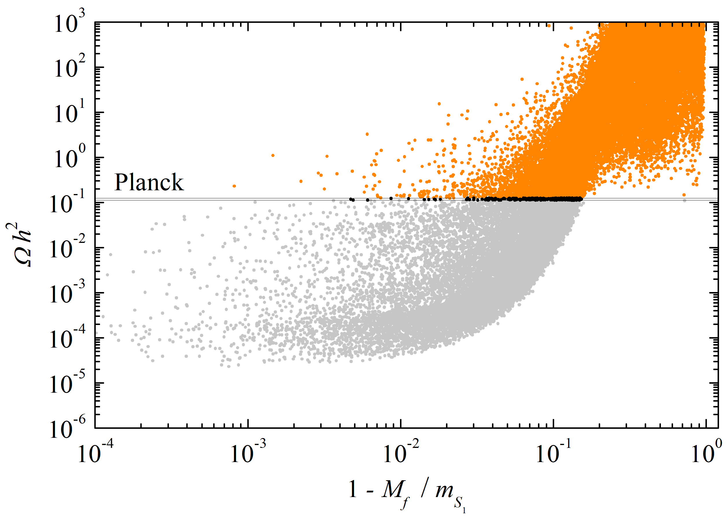

In fig. 13, we present the relic density as a function of the fermionic DM mass . We employ the same colour code of figs. 9, 11 and 12, with the addition that LEP excluded points [see eqs. (24) and discussion therein] are also indicated in grey. By looking at the black points, one concludes that correct relic density can be achieved for any value of lying above GeV. Furthermore, a similar relic density ”dip pattern” as the one of fig. 9 for scalar DM, is visible. This indicates that coannihilation decays between and the odd-scalars were included, being these crucial for achieving viable . In fact, only considering annihilation channels leads to a small thermally average cross section resulting in relic density over abundance. In fig. 14, we present as a function of the relative difference between and the mass of the lightest dark neutral (charged) scalar, (), on the left (right) plot. Globally, it can be inferred that for a relative difference inferior to , viable relic density is achieved.
Let us finally discuss the DD prospects for the fermionic DM. Since we are working in the alignment limit, i.e. , the Higgs doublet neutral scalars do not mix with . This implies the absence of tree-level contributions to the spin-independent cross section coming from the scattering of . Additionally, since is a Majorana fermion, the contributions to the electric and magnetic dipole moment identically vanish at one-loop level Herrero-Garcia:2018koq. Thus, in the alignment limit, there are no DD prospects for fermion DM. Once we allow , the fermion contributes at tree level to as show in fig. 15, thanks to the mixing between non-dark neutral scalars. The spin-independent nucleon-DM scattering cross-section in this case reads
| (46) |
where is defined in eq. (34), and
| (47) |
In the limit , the above expression reduces to
| (48) |
being defined in eq. (44). Thus, for fermion DM, can be simplified to
| (49) |
Notice that since , the dependence of on comes almost exclusively from . Also, for the contribution from the heaviest scalar to is subdominant. In such case, is required to be large enough to guarantee perturbativity for [see eq. (28) and discussion therein], leading to a further suppression of through the Yukawa coupling .
Maximizing the expression in eq. (49) with , and , leads to the bound cm2. For a more realistic case where is at its maximally-allowed value from Higgs signal rate observables at the LHC ( for GeV Ilnicka:2018def; Robens:2019ynf) and , with GeV, we obtain
| (50) |
In order to guarantee , can be at most 1.1 TeV, leading to cm2, which stands well above the current XENON1T limits.
In fig. 16, we show the contours for different values of up to the experimental limit Ilnicka:2018def; Robens:2019ynf. We conclude that, for GeV, contours with are below the XENON1T bound. Such mixing can be achieved for .
6 Concluding remarks
In this work, we have considered a SM extension where neutrino masses are generated via an interplay between the tree-level type-II seesaw and the radiative scotogenic mechanisms. The model features a flavour symmetry which leads to specific Yukawa patterns with texture zeros. Imposing CP conservation at the Lagrangian level, we show that SCPV leads to observable CP-violating effects in the lepton sector. The two texture-zero patterns for the effective neutrino mass matrix are tested in light of the most recent neutrino oscillation data. The main results and findings of our work can be summarised as follows:
- •
The imposed symmetry leads to an effective neutrino mass matrix with two texture zeros. Depending on the charges of the lepton fields, there are three different cases, namely , and , which lead to of type , and , respectively. For A1 we have , which is not compatible with IO. In this case, for NO, is constrained to be in the range (3), while is required to be in the interval meV (3) – well below the current limits from Planck cosmology and KATRIN. Significant constraints on and are obtained for B3 and B4, which select one of the octants and sharply predict . These two cases also lead to a lower limit on in the range probed by cosmology and to a neutrinoless double beta decay mass parameter within the sensitivity of current decay experiments. In particular, we have shown that the KamLAND-Zen 400 result strongly disfavours B3 (NO and IO) and B4 (IO).
- •
The three body decays and are induced by the scalars stemming from the triplet responsible for the type-II seesaw contributions to neutrino masses. Instead, the processes and are mediated at loop level by the dark-sector degrees of freedom. While these decays are possible for all cases, conversion occurs only for . We have shown that a large fraction of the model’s parameter space is excluded by current cLFV bounds, leaving some regions which will be probed by future experiments.
- •
We have studied the DM phenomenology for both the scalar and fermion cases. In the former, two viable mass regions for the lightest stable scalar are compatible with the experimental interval for the DM relic density, namely GeV and . The lower mass region is excluded by current DM DD experiments and by collider constraints from LEP on scalar masses and LHC Higgs data (invisible and diphoton decay). The intermediate mass interval is viable and will be probed by future DD searches. On the other hand, for GeV (high-mass region), our model leads to under abundant DM. This happens due to the link between dark scalar masses and scotogenic neutrino mass generation in our model (see section 3), which makes a highly-degenerate mass spectrum (required for obtaining correct for high DM masses) not natural since it would lead to non-perturbative Yukawa couplings. When the dark fermion is the lightest stable particle, a viable relic-density value is always obtained for GeV. This happens for dark fermion-scalar mass spittings below . In the alignment limit, there is no DD contribution (neither tree-level nor loop since is Majorana). Moving away from the alignment limit, non-dark neutral scalars mix, leading to tree-level contribution to the spin-independent cross section.
In conclusion, we have studied the phenomenology of a hybrid scoto-seesaw model which, albeit being based on a very simple flavour symmetry, leads to significant constraints in view of present and future data coming from neutrino, cLFV and DM experiments. We remark that the model presented here is much more restrictive and testable than that of ref. Barreiros:2020gxu. This is mainly due to the fact that, in the present case, the seesaw is of type II instead of type I as in that work.
Acknowledgements.
This work is supported by Fundação para a Ciência e a Tecnologia (FCT, Portugal) through the projects CFTP-FCT Unit UIDB/00777/2020 and UIDP/00777/2020, CERN/FIS-PAR/0004/2019 and PTDC/FIS-PAR/29436/2017, which are partially funded through POCTI (FEDER), COMPETE, QREN and EU. The work of D.B. and H.C. is supported by the PhD FCT grants SFRH/BD/137127/2018 and 2021.06340.BD, respectively.Appendix A The scalar sector
The scalar sector of our model presented in section 2 contains, besides of the usual Higgs doublet , two doublets , a scalar triplet and a complex scalar singlet , which we define as
| (51) |
with the following vacuum configuration,
| (52) |
Note that the dark scalar doublets are inert, i.e. they are VEV-less. This condition is needed to guarantee DM stability. The full scalar potential allowed by the flavour symmetry of our model (see table 1) is given by
| (53) |
with
| (54) | ||||
| (55) | ||||
| (56) | ||||
| (57) | ||||
| (58) | ||||
| (59) | ||||
| (60) | ||||
| (61) | ||||
| (62) | ||||
| (63) |
where all parameters are real. Note that we added a single soft-breaking term in eq. (56), namely which, as will be seen later, is crucial for compatibility with neutrino data and also helps avoiding the cosmological domain wall problem.
Minimisation of the scalar potential leads to four non-trivial conditions,
| (64) | ||||
| (65) | ||||
| (66) | ||||
| (67) |
These equations can be solved for , , and as a function of the VEVs , and , as well as the remaining parameters in . We obtain three distinct solutions,
| (68) | ||||
| (69) | ||||
| (i) : | (70) | |||
| (ii) : | (71) | |||
| (iii) : | (72) |
In the above, the expressions for and are common to all solutions. Note that (i) and (ii) lead to trivial phases and, therefore, the only viable solution to implement SCPV is (iii). Furthermore, if the soft-breaking parameter vanishes we will have which is still a CPV solution. However, in this model, such value of is only allowed by compatibility with neutrino data for case A1 at the 3 level. In turn, as seen in section 3, for cases B3 and B4, is fixed to values close to (), when considering best-fit values for neutrino observables to data. Therefore, a non-vanishing is required, avoiding also the domain wall problem from spontaneous breaking. The SCPV solution (72) corresponds to the global minimum of the potential if .
From eq. (69), the VEV of may be written as
| (73) |
where the hierarchy was considered. Note that, as discussed in section 2, those VEV relations are natural in the t’Hooft sense tHooft:1979rat. Also, is further suppressed for very heavy scalar triplet .
A.1 Scalar mass spectrum and scotogenic loop functions
The scalar content of our model can be divided in two classes, depending on the charge carried by the fields under the unbroken symmetry, i.e. we can have even scalars or odd dark scalars. Besides the usual pseudo-Goldstone bosons and , the even scalars are a doubly charged scalar , a charged Higgs , and five neutral scalars. The mass of is given by
| (74) |
while the mass reads,
| (75) |
In turn, the mass matrix of the non-dark neutral scalar states can be written as,
|
|
(76) |
in the basis. In order to obtain the above matrix form, we rephased the fields , and and used eqs. (68), (69) and (72) to write , , and in terms of the remaining potential parameters. The same method is used to find mass and mixing matrices for the other scalars of the model. In the limit , achieved for and small [see eq. (73)], decouple, as can be seen from eq. (76). The masses of the remaining neutral scalars can then be obtained by computing the eigenvalues of
| (77) |
written in the basis. The corresponding mixing reads
| (78) |
being a orthogonal matrix parametrised by three mixing angles and () the neutral scalar mass eigenstates.
The dark scalar sector contains two charged () and four neutral () scalars. Note that the mass-eigenstates with masses are those relevant for cLFV (see section 4). The corresponding mass matrix reads,
| (79) |
in the basis, and the respective eigenvalues are
| (80) | ||||
with , , and . The charged components of the inert doublets are related to through an orthogonal matrix as
| (81) |
being the mixing angle given by,
| (82) |
The mass-eigenstates () with masses are the ones relevant for one-loop neutrino mass generation (see sections 2 and 3). The corresponding mass matrix in the basis reads,
| (83) |
with,
|
|
(84) | ||
|
|
(85) |
being . The and masses may then be obtained by computing the eigenvalues of the matrices in eqs. (84) and (85), respectively. In the limit , we get
| (86) |
with and
| (87) |
with . In the above expressions,
| (88) |
The neutral components of the inert doublets are related to through the orthogonal matrix :
| (89) |
where the two mixing angles and are given by,
|
|
(90) |
From eq. (89), the weak-basis fields and can be written as,
| (91) |
and, thus, the scotogenic loop functions relevant for neutrino mass generation, in the mass eigenstate-basis, read:
| (92) | ||||
| (93) | ||||
| (94) |
Using the explicit expression for in terms of the mixing angles [see eq. (89)]:
| (95) | ||||
| (96) |
| (97) |
Some comments regarding the above loop-functions are in order. Notice that they depend on the masses shown in eqs. (86) and (87), as well as mixing among dark neutral states defined by the angles in eq. (90). In the limit ( decoupled from the remaining scalars), the mass differences are given by:
| (98) |
| (99) |
As seen from the above equations, the degeneracy is controlled by . If and/or are small, which, as argued, is natural in the t’Hooft sense, we have , implying . For the purposes of our analysis, we take some limiting cases of the above loop-functions. If the term proportional to is absent from the scalar potential [see eq. (60)], then while and . This implies and, thus, vanishing scotogenic contributions to neutrino masses (see fig. 1 and discussion therein). Still, cLFV mediated by dark scalars is possible since and mix. If, additionally [see eq. (62)], there is no scoto-induced cLFV [see discussion in section 4 and eq. (29)]. If only , we obtain , [see eqs. (82) and (80)], while, and . Thus, but and there is no scotogenic neutrino mass generation nor radiative cLFV. This indicates that with , as verified by our numerical analysis presented in section 4. In conclusion, when and/or , the loop-functions tend to zero faster than , and the ratio defined in eq. (17) obeys .
Appendix B Dark matter (co)annihilation diagrams
References
- (1) A.B. McDonald, Nobel Lecture: The Sudbury Neutrino Observatory: Observation of flavor change for solar neutrinos, Rev. Mod. Phys. 88 (2016) 030502.
- (2) T. Kajita, Nobel Lecture: Discovery of atmospheric neutrino oscillations, Rev. Mod. Phys. 88 (2016) 030501.
- (3) Planck collaboration, Planck 2018 results. VI. Cosmological parameters, Astron. Astrophys. 641 (2020) A6 [1807.06209].
- (4) P.F. de Salas, D.V. Forero, S. Gariazzo, P. Martínez-Miravé, O. Mena, C.A. Ternes et al., 2020 global reassessment of the neutrino oscillation picture, JHEP 02 (2021) 071 [2006.11237].
- (5) I. Esteban, M.C. Gonzalez-Garcia, M. Maltoni, T. Schwetz and A. Zhou, The fate of hints: updated global analysis of three-flavor neutrino oscillations, JHEP 09 (2020) 178 [2007.14792].
- (6) F. Capozzi, E. Di Valentino, E. Lisi, A. Marrone, A. Melchiorri and A. Palazzo, Unfinished fabric of the three neutrino paradigm, Phys. Rev. D 104 (2021) 083031 [2107.00532].
- (7) P. Minkowski, at a Rate of One Out of Muon Decays?, Phys. Lett. B 67 (1977) 421.
- (8) M. Gell-Mann, P. Ramond and R. Slansky, Complex Spinors and Unified Theories, Conf. Proc. C 790927 (1979) 315 [1306.4669].
- (9) T. Yanagida, Horizontal gauge symmetry and masses of neutrinos, Conf. Proc. C 7902131 (1979) 95.
- (10) S.L. Glashow, The Future of Elementary Particle Physics, NATO Sci. Ser. B 61 (1980) 687.
- (11) R.N. Mohapatra and G. Senjanovic, Neutrino Mass and Spontaneous Parity Nonconservation, Phys. Rev. Lett. 44 (1980) 912.
- (12) W. Konetschny and W. Kummer, Nonconservation of Total Lepton Number with Scalar Bosons, Phys. Lett. B 70 (1977) 433.
- (13) T.P. Cheng and L.-F. Li, Neutrino Masses, Mixings and Oscillations in SU(2) x U(1) Models of Electroweak Interactions, Phys. Rev. D 22 (1980) 2860.
- (14) G. Lazarides, Q. Shafi and C. Wetterich, Proton Lifetime and Fermion Masses in an SO(10) Model, Nucl. Phys. B 181 (1981) 287.
- (15) J. Schechter and J.W.F. Valle, Neutrino Masses in SU(2) x U(1) Theories, Phys. Rev. D 22 (1980) 2227.
- (16) R.N. Mohapatra and G. Senjanovic, Neutrino Masses and Mixings in Gauge Models with Spontaneous Parity Violation, Phys. Rev. D 23 (1981) 165.
- (17) M. Magg and C. Wetterich, Neutrino Mass Problem and Gauge Hierarchy, Phys. Lett. B 94 (1980) 61.
- (18) A. Rossi, Supersymmetric seesaw without singlet neutrinos: Neutrino masses and lepton flavor violation, Phys. Rev. D 66 (2002) 075003 [hep-ph/0207006].
- (19) F.R. Joaquim and A. Rossi, Gauge and Yukawa mediated supersymmetry breaking in the triplet seesaw scenario, Phys. Rev. Lett. 97 (2006) 181801 [hep-ph/0604083].
- (20) F.R. Joaquim and A. Rossi, Phenomenology of the triplet seesaw mechanism with Gauge and Yukawa mediation of SUSY breaking, Nucl. Phys. B 765 (2007) 71 [hep-ph/0607298].
- (21) M. Raidal et al., Flavour physics of leptons and dipole moments, Eur. Phys. J. C 57 (2008) 13 [0801.1826].
- (22) A. Brignole, F.R. Joaquim and A. Rossi, Beyond the standard seesaw: Neutrino masses from Kahler operators and broken supersymmetry, JHEP 08 (2010) 133 [1007.1942].
- (23) F.R. Joaquim, Running effects on neutrino parameters and l(i) — l(j) gamma predictions in the triplet-extended MSSM, JHEP 06 (2010) 079 [0912.3427].
- (24) G. Bertone and D. Hooper, History of dark matter, Rev. Mod. Phys. 90 (2018) 045002 [1605.04909].
- (25) A. Arbey and F. Mahmoudi, Dark matter and the early Universe: a review, Prog. Part. Nucl. Phys. 119 (2021) 103865 [2104.11488].
- (26) E. Ma, Verifiable radiative seesaw mechanism of neutrino mass and dark matter, Phys. Rev. D 73 (2006) 077301 [hep-ph/0601225].
- (27) A. Vicente and C.E. Yaguna, Probing the scotogenic model with lepton flavor violating processes, JHEP 02 (2015) 144 [1412.2545].
- (28) S.-Y. Guo and Z.-L. Han, Observable Signatures of Scotogenic Dirac Model, JHEP 12 (2020) 062 [2005.08287].
- (29) N.G. Deshpande and E. Ma, Pattern of Symmetry Breaking with Two Higgs Doublets, Phys. Rev. D 18 (1978) 2574.
- (30) R. Barbieri, L.J. Hall and V.S. Rychkov, Improved naturalness with a heavy Higgs: An Alternative road to LHC physics, Phys. Rev. D 74 (2006) 015007 [hep-ph/0603188].
- (31) I.M. Ávila, G. Cottin and M.A. Díaz, Revisiting the scotogenic model with scalar dark matter, 2108.05103.
- (32) M. Hirsch, R.A. Lineros, S. Morisi, J. Palacio, N. Rojas and J.W.F. Valle, WIMP dark matter as radiative neutrino mass messenger, JHEP 10 (2013) 149 [1307.8134].
- (33) S. Fraser, E. Ma and O. Popov, Scotogenic Inverse Seesaw Model of Neutrino Mass, Phys. Lett. B 737 (2014) 280 [1408.4785].
- (34) A. Ahriche, K.L. McDonald and S. Nasri, The Scale-Invariant Scotogenic Model, JHEP 06 (2016) 182 [1604.05569].
- (35) F. von der Pahlen, G. Palacio, D. Restrepo and O. Zapata, Radiative Type III Seesaw Model and its collider phenomenology, Phys. Rev. D 94 (2016) 033005 [1605.01129].
- (36) C. Hagedorn, J. Herrero-García, E. Molinaro and M.A. Schmidt, Phenomenology of the Generalised Scotogenic Model with Fermionic Dark Matter, JHEP 11 (2018) 103 [1804.04117].
- (37) C. Bonilla, L.M.G. de la Vega, J.M. Lamprea, R.A. Lineros and E. Peinado, Fermion Dark Matter and Radiative Neutrino Masses from Spontaneous Lepton Number Breaking, New J. Phys. 22 (2020) 033009 [1908.04276].
- (38) T. Nomura, H. Okada and O. Popov, A modular symmetric scotogenic model, Phys. Lett. B 803 (2020) 135294 [1908.07457].
- (39) I.M. Ávila, V. De Romeri, L. Duarte and J.W.F. Valle, Phenomenology of scotogenic scalar dark matter, Eur. Phys. J. C 80 (2020) 908 [1910.08422].
- (40) S. Centelles Chuliá, R. Cepedello, E. Peinado and R. Srivastava, Scotogenic dark symmetry as a residual subgroup of Standard Model symmetries, Chin. Phys. C 44 (2020) 083110 [1901.06402].
- (41) Z.-L. Han and W. Wang, Predictive Scotogenic Model with Flavor Dependent Symmetry, Eur. Phys. J. C 79 (2019) 522 [1901.07798].
- (42) S. Jana, P.K. Vishnu and S. Saad, Minimal dirac neutrino mass models from gauge symmetry and left–right asymmetry at colliders, Eur. Phys. J. C 79 (2019) 916 [1904.07407].
- (43) P. Escribano, M. Reig and A. Vicente, Generalizing the Scotogenic model, JHEP 07 (2020) 097 [2004.05172].
- (44) A. Beniwal, J. Herrero-García, N. Leerdam, M. White and A.G. Williams, The ScotoSinglet Model: a scalar singlet extension of the Scotogenic Model, JHEP 21 (2020) 136 [2010.05937].
- (45) P. Escribano and A. Vicente, An ultraviolet completion for the Scotogenic model, Phys. Lett. B 823 (2021) 136717 [2107.10265].
- (46) V. De Romeri, M. Puerta and A. Vicente, Dark matter in a charged variant of the Scotogenic model, 2106.00481.
- (47) F.J. de Anda, O. Medina, J.W.F. Valle and C.A. Vaquera-Araujo, Scotogenic Majorana neutrino masses in a predictive orbifold theory of flavor, Phys. Rev. D 105 (2022) 055030 [2110.06810].
- (48) N. Rojas, R. Srivastava and J.W.F. Valle, Simplest Scoto-Seesaw Mechanism, Phys. Lett. B 789 (2019) 132 [1807.11447].
- (49) S. Mandal, R. Srivastava and J.W.F. Valle, The simplest scoto-seesaw model: WIMP dark matter phenomenology and Higgs vacuum stability, Phys. Lett. B 819 (2021) 136458 [2104.13401].
- (50) D.M. Barreiros, F.R. Joaquim, R. Srivastava and J.W.F. Valle, Minimal scoto-seesaw mechanism with spontaneous CP violation, JHEP 04 (2021) 249 [2012.05189].
- (51) G.C. Branco, R.G. Felipe and F.R. Joaquim, Leptonic CP Violation, Rev. Mod. Phys. 84 (2012) 515 [1111.5332].
- (52) G. ’t Hooft, Naturalness, chiral symmetry, and spontaneous chiral symmetry breaking, NATO Sci. Ser. B 59 (1980) 135.
- (53) S. Kanemura and H. Sugiyama, Dark matter and a suppression mechanism for neutrino masses in the Higgs triplet model, Phys. Rev. D 86 (2012) 073006 [1202.5231].
- (54) A. Arhrib, R. Benbrik, M. Chabab, G. Moultaka, M.C. Peyranere, L. Rahili et al., The Higgs Potential in the Type II Seesaw Model, Phys. Rev. D 84 (2011) 095005 [1105.1925].
- (55) A. Arhrib, R. Benbrik, M. Chabab, G. Moultaka and L. Rahili, Higgs boson decay into 2 photons in the type~II Seesaw Model, JHEP 04 (2012) 136 [1112.5453].
- (56) M. Aoki, S. Kanemura, M. Kikuchi and K. Yagyu, Renormalization of the Higgs Sector in the Triplet Model, Phys. Lett. B 714 (2012) 279 [1204.1951].
- (57) M. Aoki, S. Kanemura, M. Kikuchi and K. Yagyu, Radiative corrections to the Higgs boson couplings in the triplet model, Phys. Rev. D 87 (2013) 015012 [1211.6029].
- (58) J. Alcaide, J. Salvado and A. Santamaria, Fitting flavour symmetries: the case of two-zero neutrino mass textures, JHEP 07 (2018) 164 [1806.06785].
- (59) W. Rodejohann and J.W.F. Valle, Symmetrical Parametrizations of the Lepton Mixing Matrix, Phys. Rev. D 84 (2011) 073011 [1108.3484].
- (60) P. F. De Salas, D. V. Forero, S. Gariazzo, P. Martínez-Miravé, O. Mena, C. A. Ternes et al., “Chi2 profiles from Valencia neutrino global fit.” http://globalfit.astroparticles.es/, 2021. 10.5281/zenodo.4726908.
- (61) KATRIN collaboration, Direct neutrino-mass measurement with sub-electronvolt sensitivity, Nature Phys. 18 (2022) 160 [2105.08533].
- (62) DUNE collaboration, Long-Baseline Neutrino Facility (LBNF) and Deep Underground Neutrino Experiment (DUNE): Conceptual Design Report, Volume 2: The Physics Program for DUNE at LBNF, 1512.06148.
- (63) Hyper-Kamiokande Working Group collaboration, A Long Baseline Neutrino Oscillation Experiment Using J-PARC Neutrino Beam and Hyper-Kamiokande, 12, 2014 [1412.4673].
- (64) EXO-200 collaboration, Search for Neutrinoless Double- Decay with the Complete EXO-200 Dataset, Phys. Rev. Lett. 123 (2019) 161802 [1906.02723].
- (65) GERDA collaboration, Final Results of GERDA on the Search for Neutrinoless Double- Decay, Phys. Rev. Lett. 125 (2020) 252502 [2009.06079].
- (66) CUORE collaboration, Search for Majorana neutrinos exploiting millikelvin cryogenics with CUORE, Nature 604 (2022) 53 [2104.06906].
- (67) KamLAND-Zen collaboration, Search for Majorana Neutrinos near the Inverted Mass Hierarchy Region with KamLAND-Zen, Phys. Rev. Lett. 117 (2016) 082503 [1605.02889].
- (68) AMoRE collaboration, AMoRE: A search for neutrinoless double-beta decay of 100Mo using low-temperature molybdenum-containing crystal detectors, JINST 15 (2020) C08010 [2005.05567].
- (69) CUPID collaboration, CUPID: CUORE (Cryogenic Underground Observatory for Rare Events) Upgrade with Particle IDentification, 1504.03599.
- (70) LEGEND collaboration, The Large Enriched Germanium Experiment for Neutrinoless Double Beta Decay (LEGEND), AIP Conf. Proc. 1894 (2017) 020027 [1709.01980].
- (71) nEXO collaboration, Sensitivity and Discovery Potential of nEXO to Neutrinoless Double Beta Decay, Phys. Rev. C 97 (2018) 065503 [1710.05075].
- (72) X. Chen et al., PandaX-III: Searching for neutrinoless double beta decay with high pressure136Xe gas time projection chambers, Sci. China Phys. Mech. Astron. 60 (2017) 061011 [1610.08883].
- (73) SNO+ collaboration, Current Status and Future Prospects of the SNO+ Experiment, Adv. High Energy Phys. 2016 (2016) 6194250 [1508.05759].
- (74) A. Pich, A. Santamaria and J. Bernabeu, MU- — E- + GAMMA DECAY IN THE SCALAR TRIPLET MODEL, Phys. Lett. B 148 (1984) 229.
- (75) E. Ma, M. Raidal and U. Sarkar, Phenomenology of the neutrino mass giving Higgs triplet and the low-energy seesaw violation of lepton number, Nucl. Phys. B 615 (2001) 313 [hep-ph/0012101].
- (76) A.G. Akeroyd, M. Aoki and H. Sugiyama, Lepton Flavour Violating Decays tau — anti-l ll and mu — e gamma in the Higgs Triplet Model, Phys. Rev. D 79 (2009) 113010 [0904.3640].
- (77) J. Chakrabortty, P. Ghosh and W. Rodejohann, Lower Limits on from New Measurements on , Phys. Rev. D 86 (2012) 075020 [1204.1000].
- (78) D.N. Dinh and S.T. Petcov, Lepton Flavor Violating Decays in TeV Scale Type I See-Saw and Higgs Triplet Models, JHEP 09 (2013) 086 [1308.4311].
- (79) P.S. Bhupal Dev, D.K. Ghosh, N. Okada and I. Saha, 125 GeV Higgs Boson and the Type-II Seesaw Model, JHEP 03 (2013) 150 [1301.3453].
- (80) S. Antusch, O. Fischer, A. Hammad and C. Scherb, Low scale type II seesaw: Present constraints and prospects for displaced vertex searches, JHEP 02 (2019) 157 [1811.03476].
- (81) R. Primulando, J. Julio and P. Uttayarat, Scalar phenomenology in type-II seesaw model, JHEP 08 (2019) 024 [1903.02493].
- (82) T. Toma and A. Vicente, Lepton Flavor Violation in the Scotogenic Model, JHEP 01 (2014) 160 [1312.2840].
- (83) MEG collaboration, Search for the lepton flavour violating decay with the full dataset of the MEG experiment, Eur. Phys. J. C 76 (2016) 434 [1605.05081].
- (84) MEG II collaboration, The design of the MEG II experiment, Eur. Phys. J. C 78 (2018) 380 [1801.04688].
- (85) BaBar collaboration, Searches for Lepton Flavor Violation in the Decays tau+- — e+- gamma and tau+- — mu+- gamma, Phys. Rev. Lett. 104 (2010) 021802 [0908.2381].
- (86) Belle-II collaboration, The Belle II Physics Book, PTEP 2019 (2019) 123C01 [1808.10567].
- (87) SINDRUM collaboration, Search for the Decay mu+ — e+ e+ e-, Nucl. Phys. B 299 (1988) 1.
- (88) A. Blondel et al., Research Proposal for an Experiment to Search for the Decay , 1301.6113.
- (89) K. Hayasaka et al., Search for Lepton Flavor Violating Tau Decays into Three Leptons with 719 Million Produced Tau+Tau- Pairs, Phys. Lett. B 687 (2010) 139 [1001.3221].
- (90) Mu2e collaboration, Mu2e Technical Design Report, 1501.05241.
- (91) COMET collaboration, COMET Phase-I Technical Design Report, PTEP 2020 (2020) 033C01 [1812.09018].
- (92) SINDRUM II collaboration, Test of lepton flavor conservation in mu — e conversion on titanium, Phys. Lett. B 317 (1993) 631.
- (93) A. Alekou et al., Accelerator system for the PRISM based muon to electron conversion experiment, in Community Summer Study 2013: Snowmass on the Mississippi, 10, 2013 [1310.0804].
- (94) SINDRUM II collaboration, A Search for muon to electron conversion in muonic gold, Eur. Phys. J. C 47 (2006) 337.
- (95) SINDRUM II collaboration, Improved limit on the branching ratio of mu — e conversion on lead, Phys. Rev. Lett. 76 (1996) 200.
- (96) Particle Data Group collaboration, Review of Particle Physics, PTEP 2020 (2020) 083C01.
- (97) G.K. Leontaris, K. Tamvakis and J.D. Vergados, Lepton and Family Number Violation From Exotic Scalars, Phys. Lett. B 162 (1985) 153.
- (98) J. Bernabeu, A. Pich and A. Santamaria, CP Phases in the Charged Current and Higgs Sectors for Majorana Neutrinos, Z. Phys. C 30 (1986) 213.
- (99) S.M. Bilenky and S.T. Petcov, Massive Neutrinos and Neutrino Oscillations, Rev. Mod. Phys. 59 (1987) 671.
- (100) Q.-H. Cao, E. Ma and G. Rajasekaran, Observing the Dark Scalar Doublet and its Impact on the Standard-Model Higgs Boson at Colliders, Phys. Rev. D 76 (2007) 095011 [0708.2939].
- (101) M. Gustafsson, E. Lundstrom, L. Bergstrom and J. Edsjo, Significant Gamma Lines from Inert Higgs Dark Matter, Phys. Rev. Lett. 99 (2007) 041301 [astro-ph/0703512].
- (102) A. Pierce and J. Thaler, Natural Dark Matter from an Unnatural Higgs Boson and New Colored Particles at the TeV Scale, JHEP 08 (2007) 026 [hep-ph/0703056].
- (103) ATLAS collaboration, Search for doubly-charged Higgs bosons in like-sign dilepton final states at TeV with the ATLAS detector, Eur. Phys. J. C 72 (2012) 2244 [1210.5070].
- (104) CMS collaboration, Inclusive search for doubly charged higgs in leptonic final states at sqrt s=7 TeV, .
- (105) ATLAS collaboration, Search for anomalous production of prompt same-sign lepton pairs and pair-produced doubly charged Higgs bosons with TeV collisions using the ATLAS detector, JHEP 03 (2015) 041 [1412.0237].
- (106) CMS collaboration, Search for a doubly-charged Higgs boson with collisions at the CMS experiment, .
- (107) ATLAS collaboration, Search for doubly charged Higgs boson production in multi-lepton final states with the ATLAS detector using proton–proton collisions at , Eur. Phys. J. C 78 (2018) 199 [1710.09748].
- (108) CMS collaboration, A search for doubly-charged Higgs boson production in three and four lepton final states at , .
- (109) ATLAS collaboration, Search for doubly charged scalar bosons decaying into same-sign boson pairs with the ATLAS detector, Eur. Phys. J. C 79 (2019) 58 [1808.01899].
- (110) K. Huitu, J. Maalampi, A. Pietila and M. Raidal, Doubly charged Higgs at LHC, Nucl. Phys. B 487 (1997) 27 [hep-ph/9606311].
- (111) A.G. Akeroyd and M. Aoki, Single and pair production of doubly charged Higgs bosons at hadron colliders, Phys. Rev. D 72 (2005) 035011 [hep-ph/0506176].
- (112) S. Kanemura, D. Nomura and K. Tsumura, Dimension-six top-Higgs interaction and its effect in collider phenomenology, Phys. Rev. D 74 (2006) 076007 [hep-ph/0607333].
- (113) A. Melfo, M. Nemevsek, F. Nesti, G. Senjanovic and Y. Zhang, Type II Seesaw at LHC: The Roadmap, Phys. Rev. D 85 (2012) 055018 [1108.4416].
- (114) F. del Águila and M. Chala, LHC bounds on Lepton Number Violation mediated by doubly and singly-charged scalars, JHEP 03 (2014) 027 [1311.1510].
- (115) K.S. Babu and S. Jana, Probing Doubly Charged Higgs Bosons at the LHC through Photon Initiated Processes, Phys. Rev. D 95 (2017) 055020 [1612.09224].
- (116) E.J. Chun, S. Khan, S. Mandal, M. Mitra and S. Shil, Same-sign tetralepton signature at the Large Hadron Collider and a future collider, Phys. Rev. D 101 (2020) 075008 [1911.00971].
- (117) R. Padhan, D. Das, M. Mitra and A. Kumar Nayak, Probing doubly and singly charged Higgs bosons at the collider HE-LHC, Phys. Rev. D 101 (2020) 075050 [1909.10495].
- (118) T.B. de Melo, F.S. Queiroz and Y. Villamizar, Doubly Charged Scalar at the High-Luminosity and High-Energy LHC, Int. J. Mod. Phys. A 34 (2019) 1950157 [1909.07429].
- (119) S. Ashanujjaman and K. Ghosh, Revisiting type-II see-saw: present limits and future prospects at LHC, JHEP 03 (2022) 195 [2108.10952].
- (120) F. Staub, SARAH 4 : A tool for (not only SUSY) model builders, Comput. Phys. Commun. 185 (2014) 1773 [1309.7223].
- (121) F. Staub, Exploring new models in all detail with SARAH, Adv. High Energy Phys. 2015 (2015) 840780 [1503.04200].
- (122) W. Porod, SPheno, a program for calculating supersymmetric spectra, SUSY particle decays and SUSY particle production at e+ e- colliders, Comput. Phys. Commun. 153 (2003) 275 [hep-ph/0301101].
- (123) W. Porod and F. Staub, SPheno 3.1: Extensions including flavour, CP-phases and models beyond the MSSM, Comput. Phys. Commun. 183 (2012) 2458 [1104.1573].
- (124) W. Porod, F. Staub and A. Vicente, A Flavor Kit for BSM models, Eur. Phys. J. C 74 (2014) 2992 [1405.1434].
- (125) G. Bélanger, F. Boudjema, A. Pukhov and A. Semenov, micrOMEGAs4.1: two dark matter candidates, Comput. Phys. Commun. 192 (2015) 322 [1407.6129].
- (126) F. Staub, T. Ohl, W. Porod and C. Speckner, A Tool Box for Implementing Supersymmetric Models, Comput. Phys. Commun. 183 (2012) 2165 [1109.5147].
- (127) M.A. Díaz, B. Koch and S. Urrutia-Quiroga, Constraints to Dark Matter from Inert Higgs Doublet Model, Adv. High Energy Phys. 2016 (2016) 8278375 [1511.04429].
- (128) A. Belyaev, G. Cacciapaglia, I.P. Ivanov, F. Rojas-Abatte and M. Thomas, Anatomy of the Inert Two Higgs Doublet Model in the light of the LHC and non-LHC Dark Matter Searches, Phys. Rev. D 97 (2018) 035011 [1612.00511].
- (129) E.C.F.S. Fortes, A.C.B. Machado, J. Montaño and V. Pleitez, Scalar dark matter candidates in a two inert Higgs doublet model, J. Phys. G 42 (2015) 105003 [1407.4749].
- (130) V. Keus, S.F. King, S. Moretti and D. Sokolowska, Observable Heavy Higgs Dark Matter, JHEP 11 (2015) 003 [1507.08433].
- (131) A. Cordero-Cid, J. Hernández-Sánchez, V. Keus, S.F. King, S. Moretti, D. Rojas et al., CP violating scalar Dark Matter, JHEP 12 (2016) 014 [1608.01673].
- (132) J. Hernandez-Sanchez, V. Keus, S. Moretti, D. Rojas-Ciofalo and D. Sokolowska, Complementary Probes of Two-component Dark Matter, 2012.11621.
- (133) A. Aranda, D. Hernández-Otero, J. Hernández-Sanchez, V. Keus, S. Moretti, D. Rojas-Ciofalo et al., Z3 symmetric inert ( 2+1 )-Higgs-doublet model, Phys. Rev. D 103 (2021) 015023 [1907.12470].
- (134) W. Khater, A. Kunčinas, O.M. Ogreid, P. Osland and M.N. Rebelo, Dark matter in three-Higgs-doublet models with S3 symmetry, JHEP 01 (2022) 120 [2108.07026].
- (135) G. Belanger, F. Boudjema, A. Pukhov and A. Semenov, Dark matter direct detection rate in a generic model with micrOMEGAs 2.2, Comput. Phys. Commun. 180 (2009) 747 [0803.2360].
- (136) LUX collaboration, Results from a search for dark matter in the complete LUX exposure, Phys. Rev. Lett. 118 (2017) 021303 [1608.07648].
- (137) PandaX-II collaboration, Dark Matter Results from First 98.7 Days of Data from the PandaX-II Experiment, Phys. Rev. Lett. 117 (2016) 121303 [1607.07400].
- (138) XENON collaboration, Dark Matter Search Results from a One Ton-Year Exposure of XENON1T, Phys. Rev. Lett. 121 (2018) 111302 [1805.12562].
- (139) LUX-ZEPLIN collaboration, Projected WIMP sensitivity of the LUX-ZEPLIN dark matter experiment, Phys. Rev. D 101 (2020) 052002 [1802.06039].
- (140) J. Billard, L. Strigari and E. Figueroa-Feliciano, Implication of neutrino backgrounds on the reach of next generation dark matter direct detection experiments, Phys. Rev. D 89 (2014) 023524 [1307.5458].
- (141) DARWIN collaboration, DARWIN: towards the ultimate dark matter detector, JCAP 11 (2016) 017 [1606.07001].
- (142) PandaX collaboration, Dark matter direct search sensitivity of the PandaX-4T experiment, Sci. China Phys. Mech. Astron. 62 (2019) 31011 [1806.02229].
- (143) XENON collaboration, Projected WIMP sensitivity of the XENONnT dark matter experiment, JCAP 11 (2020) 031 [2007.08796].
- (144) J. Billard et al., Direct Detection of Dark Matter – APPEC Committee Report, 2104.07634.
- (145) ATLAS, CMS collaboration, Measurements of the Higgs boson production and decay rates and constraints on its couplings from a combined ATLAS and CMS analysis of the LHC pp collision data at and 8 TeV, JHEP 08 (2016) 045 [1606.02266].
- (146) ATLAS collaboration, Combined measurements of Higgs boson production and decay using up to fb-1 of proton-proton collision data at 13 TeV collected with the ATLAS experiment, Phys. Rev. D 101 (2020) 012002 [1909.02845].
- (147) CMS collaboration, Search for invisible decays of a Higgs boson produced through vector boson fusion in proton-proton collisions at 13 TeV, Phys. Lett. B 793 (2019) 520 [1809.05937].
- (148) ATLAS collaboration, Measurements of Higgs boson properties in the diphoton decay channel with 36 fb-1 of collision data at TeV with the ATLAS detector, Phys. Rev. D 98 (2018) 052005 [1802.04146].
- (149) A. Ilnicka, T. Robens and T. Stefaniak, Constraining Extended Scalar Sectors at the LHC and beyond, Mod. Phys. Lett. A 33 (2018) 1830007 [1803.03594].
- (150) T. Robens, Investigating extended scalar sectors at current and future colliders, PoS LHCP2019 (2019) 138 [1908.10809].
- (151) J. Herrero-Garcia, E. Molinaro and M.A. Schmidt, Dark matter direct detection of a fermionic singlet at one loop, Eur. Phys. J. C 78 (2018) 471 [1803.05660].