Relaxation and dynamics of high-stress pre-displaced string resonators
Abstract
Pre-displaced micromechanical resonators made from high-stress material give rise to new rich static and dynamic behavior. Here, an analytical model is presented to describe the mechanics of such pre-displaced resonators. The bending and tension energies are derived and a modified Euler-Bernoulli equation is obtained by applying the least action principle. By projecting the model onto a cosine shape, the energy landscape is visualized, and the pre-displacement dependence of stress and frequency is studied semi-analytically. The analysis is extended with finite-element simulations, including the mode shape, the role of overhang, and the stress distribution.
I Introduction
Nowadays, micro and nanomechanical resonators are widely used for a large variety of applications, ranging from sensing and detection Westerveld et al. 2021; Calleja et al. 2012; Waggoner and Craighead 2007, optical and microwave quantum transducers in hybrid opto-electro-mechanical systems Lauk et al. 2020, to fundamental experiments in the quantum regime O’Connell et al. 2010; Chan et al. 2011; Fiaschi et al. 2021. These resonators are often made out of pre-strained films, like Si3N4 , as such materials provide very high quality factors Poot et al. 2015; Høj et al. 2021; Unterreithmeier et al. 2010; Norte et al. 2016, enabling e.g. high detection efficiencies in the case of sensors Waggoner and Craighead 2007 and long coherence times in mechanical quantum storage Heinrich et al. 2021. For all these experiments, it is imperative to engineer the geometry of the resonator Eichenfield et al. 2009; Høj et al. 2021; Poot and Tang 2014; Bagheri et al. 2013; Cole et al. 2011; Fong et al. 2019; Bereyhi et al. 2021 including the stress Ghadimi et al. 2018; Beccari et al. 2022, to reach the best performance. Our recent work Hoch et al. 2022 experimentally demonstrates the geometrical tuning of the stress of resonators made out of pre-strained SiN films. This not only provides a new approach for a systematic study of dissipation dilution Unterreithmeier et al. 2010; Schmid et al. 2011 but also raises interesting questions, like their potential to buckle and the influence of the geometry on the eigenmodes. A thorough study of the statics and dynamics of these structures is, however, still lacking.
Here, we provide a detailed analysis of the mechanics of pre-displaced beam resonators using analytical methods which are supported by finite-element simulations. In Sec. II the stress relaxation of straight and pre-displaced high-stress beams is studied, as well as their potential to buckle. In Sec. III, expressions for the bending and tension energy stored in the beam are derived. Based on this, their equations of motion - i.e. modified Euler-Bernoulli equations - are obtained in Sec. IV. For a deeper understanding, the model is projected onto the mode shape resembling the fundamental mode (Sec. V). Finally, in Sec. VI, finite elements simulations are used to validate the results and to study the role of the overhang, the mode shape, and the distribution of the stress throughout the beams.
II Relaxation

II.1 Relaxation of straight strings
Nanomechanical strings are typically made by etching a thin film, most notably silicon nitride, with a large, uniform tensile stress, followed by their release from the supporting substrate. The films are typically thin (thickness length ) so that the out-of-plane components (i.e., ; see Fig. 1(a) for the coordinate system) of the stress tensor vanish ( for ), and only in-plane tensile forces remain. For an isotropic material, there are no shear stresses and only the components remain. The film stress is a property of the growth process and can be controlled using e.g. the stoichiometry of the material. It is the amount of stress that remains present for two-dimensional resonators that are clamped on all sides, such as membranes Hoch et al. 2021, or when narrow (width ) and straight structures are patterned but still held by the supporting substrate as illustrated in the top panel of Fig. 1(a). After release, the forces in the direction cannot be sustained and [Fig. 1(a) center]. In this case, is, thus, the only remaining stress component, and we define its value as . Since the straight beam is clamped at the ends, the length before and after the release remains the same [see Fig. 1(a)] and thus the xx-component of the strain tensor, is identical before and after the release. For an isotropic linear-elastic material with Young’s modulus and Poison ratio , this longitudinal strain is given by , which is before and after the release. Since these two are equal, the remaining xx-component of the stress tensor can be determined: . For our silicon nitride films with and , this yields (see Appendix), corresponding to a pre-strain . Note that the cross sectional area can always be used to convert back and forth between the stress and tension .
Finally, when the clamping at and would be removed [Fig. 1(a) bottom], the beam would relax completely so that also , and the beam would attain a length . To put this into perspective: a long beam would shrink by when freed.
II.2 Relaxation of pre-displaced strings
So far, the discussion of relaxation of high-stress beams has focused on straight strings. Figure 1(b) shows a schematic of our pre-displaced strings Hoch et al. 2022. Here, the beam is made with a center line that is not straight, but has a x-dependent displacement in the y-direction . The length of the beam is thus longer than then distance between the clamping points ; the exact length depends both on and as will be shown in the next Section. Before release, the beam is supported [Fig. 1(b) top] and the stress is again . Now, upon release both transverse relaxation, as well as straightening of its shape will occur. Both will happen together, but for the understanding it is good to imagine this as two separate steps: one where the transverse stress relaxes like was shown in Fig. 1(a), but still retaining the pre-displacement, and a second one where the pre-displacement relaxes too. After the first step, the relaxed stress would also be , just like for a straight beam, but now along the direction of the center line, which can be locally under an angle with the x-axis. There will thus be an uncompensated y-component in the tension along the string, which will cause the straightening changing the profile to [Fig. 1(b) middle]. As we will detail in the following sections, how much the string straightens depends on the competition between tension and bending energy, and if there is potential to buckle.
II.3 Potential to buckle
Buckling is the sudden deformation of a structure under a compressive load, which can lead to out-of-plane deformations Etaki et al. 2008; Erbil et al. 2020; Nayfeh et al. 1995. In engineering, buckling may result in catastrophic failure of structures, but in micromechanics buckling can also be harnessed to implement a variety of functions in micromechanical devices, e.g. for information storage Charlot et al. 2008; Bagheri et al. 2011 or to control propagation of waves Kim et al. 2021. As explained above, when pre-displaced strings relax towards the line connecting the clamping points, their curve length shortens and the tensile stress decreases. When the string would be (actively made) straight between the clamping points [see Fig. 1(b) bottom], the tension can become negative, and out-of-plane deformations - cf. buckling in the z-direction - may be energetically favorable compared to in-plane deformations for . In this Section we explore if this situation can occur, or not.
The curve length of the resonator depends on the in- and out-of-plane displacement profiles, and , respectively, through the functional
| (1) |
Throughout this paper, it is assumed that the displacements are not large, e.g. and and likewise for and . In this approximation, the length becomes
| (2) |
Now, if the string would be completely straight (cf. and ), then the curve length should equal the distance between the clamping points: , which is not necessarily equal to the length that the straightened string would have if is was not clamped, , thus resulting in a strain that can be positive or negative, depending on whether is smaller or larger than . For there is still tensile strain and no buckling occurs. However, if there is a compressive load exerted by the clamping points. Still, out-of-plane buckling may only occur when that compression is large enough, i.e., when the critical strain Poot and van der Zant 2012 is exceeded: .
Figure 1(c) shows a color plot of the strain when beams with varying length and varying pre-displacements would be made straight, as well as the line where the critical strain is reached (dashed line). Long beams with small initial displacements (upper left corner) still have tensile strain when made straight, but short beams with a large displacement (lower right corner) would have compressive strain that can exceed the critical strain. Even though in Fig. 1(c) there was a large tensile stress present before release, this shows that there are still beams that have the potential to buckle, and, thus, also the out-of-plane displacement should be taken into account in the analysis.
III Bending and tension energy
To understand the statics and dynamics of the pre-displaced strings, the potential energy that is stored in both the bending and stretching of the beam is needed. In this section, first the bending energy is calculated, followed by the tension energy .
III.1 Bending energy
It costs energy to deform a mechanical structure and a part of that is due to bending. For example, when a doubly-clamped beam is displaced downwards, in the middle its bottom surface will be stretched, whereas its top becomes compressed Cleland 2003; Landau and Lifshitz 1986. Only the neutral plane does not deform. There, not only the direction of the in-plane displacement , but also the displacement-induced stretching force (concretely , see Sec. III.2) reverses sign there, so that both in the stretched and in the compressed area, elastic energy is stored. By averaging the work needed over the cross section of the beam, one obtains Cleland 2003; Poot and van der Zant 2012; Unterreithmeier et al. 2010
| (3) |
where is the bending rigidity (also known as the flexural rigidity) and is the second moment of area which equals for a beam with a rectangular cross section displaced in the z-direction Cleland 2003. The quotes in Eq. (3) denote derivatives with respect to ; the bending energy thus depends on the curvature of the displacement profile, , squared.
In the case of a tensionless beam with a pre-displacement in the y direction , the same argument can be used to find the bending energy for the in-plane direction:
| (4) |
with and . For , the bending energy is at its minimum: and the more the beam displaces from its initial shape the more bending energy this costs. The total bending energy is the sum of and .
III.2 Tension energy
Compared to , the tension energy is more subtle to calculate since, in addition to a constant component , a part of the tension depends on the flexural displacements. First focusing on in-plane displacements only, one can ask what force distribution generates a particular , given a tension . The static force balance of a string under tension is Poot and van der Zant 2012
| (5) |
This is typically used to find the displacement for a given force distribution by solving the differential equation, but when is already specified, the force per unit length that is needed to create that displacement can be obtained from Eq. (5) directly. is thus a functional of the displacement profile, we indicate this with . Eq. (5) shows that the larger the displacement, the larger the force per unit length has to be.
Physically, originates from the tension that tries to pull the string back to . When incrementing the displacement, work is done against that tension, which is stored as potential energy. By summing the work required to bring the displacement from 0 to , and integrating over the length of the string, one obtains:
| (6) |
By using Eq. (5) and defining , Eq. (6) can be expressed as
| (7) | |||||
| (8) |
Note, that the second integral in Eq. (8) only contains the final displacement profile and its curvature, whereas the first integral takes the changing magnitude of the displacement and tension during the process of going from to into account through the dummy variable . If the tension would be independent of , i.e., , then the integral over would give Unterreithmeier et al. 2010. With the contribution because of the displacement-induced elongation of Eq. (2) included, the tension is
| (9) |
The second term in Eq. (9) gives an additional , so that appears in the anti-derivative of the first integrant of Eq. (8). The prefactor of that term is instead of the in front of in the expression from . Here, it should be emphasized again that is the tension of the straight beam , and not the tension initially present after the transverse stress relaxation, as was detailed in Sec. II.2. Still, after inserting into Eq. (9) and rearranging, one obtains
| (10) |
which shows clearly that depends on the pre-displacement and on the initial stress .
After performing partial integration and realizing that the boundary terms are zero for the boundary conditions , the tension energy becomes:
| (11) |
It should be noted that the “effective” tension appearing between the curly brackets in is neither the initial tension , nor the final tension , but . When is positive, , i.e. straight strings, is a minimum of . When the effective tension is negative, corresponds to a maximum in and buckling may occur, as explored in Sec. II.3. From Eq. (9) it is clear that this requires .
When both displacements in the y- () and z-direction () are present, the tension is a functional of both profiles, , and after a similar derivation as done above for only, the tension energy becomes:
| (12) |
with .
IV Equations of motion
The equation of motion for and can be obtained using the formalism of Lagrangian mechanics Wells 1967. For this, the total potential energy , as derived in the previous Section, as well as the kinetic energy are needed. The latter is:
| (13) |
where the dot indicates a derivative w.r.t. time .
To obtain the equations of motion, in short, one inserts (and likewise for ) into the Lagrangian and linearizes in the infinitesimal virtual displacement . This results in integrals containing , as well as its time (in ) and spatial derivatives (in , , and ). And after performing partial integration, and setting the total change in the Lagrangian to zero, one obtains an equation with an integral over the beam length containing itself, but no longer its derivatives. Since should hold for arbitrary , the prefactor of inside the integral should vanish at all locations . This yields to the Euler-Bernoulli equations Cleland 2003; Landau and Lifshitz 1986 with tension included Nayfeh et al. 1995; Poot et al. 2007; Westra et al. 2010; Unterreithmeier et al. 2010, but now with the fourth order spatial derivative of instead of :
| (14) | |||||
| (15) |
Here, external forces (per unit length) in the y and z direction ( and ) have also been included. Note, that the actual tension appears again Nayfeh et al. 1995, and not the effective tension appearing as prefactor in [see Eq. (12)]. This is because the virtual work done by the virtual displacement not only contains the direct change via the integral of Eq. (12), but also the change . This is analogous to the emergence of the ac tension Westra et al. 2010 in description of the flexural resonances of carbon nanotubes Poot et al. 2007 and buckled beams Etaki et al. 2008. The fact that only appears in the equation of motion is expected, since in a local force balance - which would also lead to Eqs. (14)-(15) - it is irrelevant if the tension is due to , due to the elongation, or a combination of the two.
A dimension analysis Poot et al. 2007 shows that is the parameter that determines the importance of tension over bending rigidity. A resonator with behaves as a string, whereas one with acts as a tensionless beam. Interestingly, when the “stringness” Hoch et al. 2022 , i.e. a resonator where the tension dominates over the bending rigidity, drops out of Eq. (14). Thus, after relaxing, the pre-displaced beams simply behave as strings under tension and the only effect of the pre-displacement will be the geometric tuning of the tension Hoch et al. 2022. Irrespective of the value of , the term in Eq. (14) is independent of and and, hence, when solving the equations of motion, that term can be viewed as an additional in-plane force per unit length that acts on the beam. Thus, to solve the static displacement and the eigenmodes, one can follow the standard approach of inserting and solving for the static profile and for the eigenmodes by taking . In the latter case, it is important to also include the ac part of the tension Poot et al. 2007. Although the mode shapes can be solved analytically, finding the tension and eigenvalues typically has to be done numerically Poot et al. 2007; Hoch et al. 2022.
V Projection onto modes
The full equations of motion [Eqs. (14) and (15)] are partial differential equations that govern both the spatial profile and the dynamics. Getting insights from these directly is therefore not easy. The analysis can be greatly simplified by assuming a specific displacement profile and projecting onto that mode. Of course, the better that Ansatz is, the better the agreement between the dynamics calculated using the full and the reduced equations of motion will be. In our experimental work Hoch et al. 2022, the focus was on the so-called “Sbeam” design that is close to the cosine shape. Inspired by this, we take
| (16) |
for the pre- and post-release in-plane displacement and the out-of-plane displacement, respectively. Note that displacement profiles of the form (16) satisfy the boundary conditions for doubly-clamped beams Cleland 2003 and also correspond to the shape of buckled beams Poot and van der Zant 2012. With a single anti-node at , they also resemble the shape of the fundamental in- and out-of-plane flexural modes of beams and strings. On the other hand, Eq. (16) is not expected to work well for higher modes which have very different shapes, e.g with more nodes. For these, different projections for the static and dynamic behaviour may be used Westra et al. 2010. Alternatively the full model [Eqs. (14) and (15)] can be solved, or finite-element simulation can be performed. However, in the following we focus on the fundamental modes. Inserting Eq. (16) into the expression for , , , and , and performing the integration yields:
| (17) | |||||
| (18) | |||||
| (19) | |||||
| (20) |
where is the total mass of the beam Poot and van der Zant 2012. The factors after the multiplication sign depend on the assumed displacement profile. If, for example, instead of , was chosen (i.e. the fundamental mode shape of a string, as well as the pre-displacement of our “sine” design Hoch et al. 2022) these factors would be , , , and , respectively. In words, for the same amount of center displacement, it would have less bending energy, but equal stretching energy and tension as well as a higher effective mass . In the following, we employ on the shape given by Eq. (16) for the projection onto the modes; this agrees well with finite-element simulations as will be shown below.
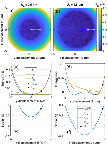
V.1 Potential energy landscape
After the projection onto the mode shape using Eq. (16), the total potential energy is a function of the two center displacements, and . Figure 2(a) and (b) show this two-dimensional energy landscape for beams with two different center pre-displacements . First of all, note that both potentials are symmetric with respect to . This can be understood because only appears in Eqs. (17)-(20). Moreover, both panels show that it costs energy to displace the beam beyond and that the potential energy can be lowered by straightening (). Still, they show very different behaviour: For , the potential energy contours appear almost concentric, and the relaxed displacement, given by the position of the potential minimum , is close to 0. Figure. 2(c) indicates that in this case the tension energy (blue) dominates over the bending energy (green) and that after straightening the string still has a considerable positive strain value [Fig. 2(e)]. For , the beam thus almost completely straightens and still has considerable tensile stress after relaxing.
For , the situation is different. In this case, the potential landscape is more complex as both the contour plot in (b) and the line cuts in (d) show. From the latter, appears to have two minima, but, as panel (b) shows, the left one is actually a saddle point. The global minimum is at , which indicates that there is still a significant bending. In other words, the beam has not fully straightened. Looking at the strain in Fig. 2(f) clarifies that would be a situation with a compressive strain that exceeds the critical value for buckling (see Sec. II.3). Indeed, looking back at Fig. 1(c) shows that the beam with does not have the potential to buckle, whereas the one with has. In the latter case, the beam thus remains displaced, but has only very small (tensile) stress after relaxing. Note that there is no out-of-plane displacement, which would be ; in our numerical studies that situation was only encountered for compressive initial stress . Even for , with tensile film stress the pre-displaced beams thus “prefer” an in-plane displacement above out-of plane buckling. Still, the potential to buckle as introduced in Sec. II.3 is an important parameter that indicates if the beams will almost completely straighten, or not.

V.2 Pre-displacement dependence
The position of the minimum in the potential energy can be tracked as a function of the pre-displacement . With its value, also the relaxed tension can be calculated from Eq. (20). Figure 3(a) and (b) show and the tension normalized by the cross sectional area, respectively. These show that, in agreement with the experiments Hoch et al. 2022, for , the final displacement is close to zero and that the stress is still relatively large. The latter is close to that of a straight string , as calculated using Eq. (10) (dotted). Beyond where becomes zero, the stress becomes small - but is still tensile - and the displacement grows. Interestingly, the relaxed displacement approaches that of a buckled beam under compressive tension (dotted line) Nayfeh et al. 1995. This shows once more that the behaviour of the beams is intimately related to their potential to buckle. Both before, after, and close to the buckling transition, both the final stress and displacement obtained from the analytical modal-projection model are almost indistinguishable from those obtained using finite-element simulations (FEM, dashed lines). This shows that the analytical model can be used to accurately describe the static relaxation of the pre-displaced beams.
V.3 Reduced equations of motion
To derive the reduced equations of motion, i.e. the differential equations that govern the dynamics of the center displacements and , the formalism of Hamiltonian mechanics is employed. There, Hamilton’s equations relates the generalized momenta and that are associated with and , respectively, to derivatives of the Hamiltonian with respect to said quantities, and vice versa Wells 1967:
| (21) | |||||
| (22) |
From this, the reduced equations of motion follow directly:
| (23) | |||||
| (24) | |||||
Here, is again the effective mass. Comparing these equations to the equation of motion for a harmonic oscillator shows that the part of the right hand sides that is proportional to and , respectively, contains the spring constants and these determine the resonance frequencies. Both the first (i.e. bending) and second (tension, via ) term contribute to this. Besides these linear contributions, there are e.g. also terms proportional to and . The last term in Eqs. (23) and (24) is clearly nonlinear, but, since the tension depends on and [see Eq. (20)], also the second term contributes to the beam’s nonlinearities. This term also nonlinearly couples in- and out-of-plane motion Westra et al. 2010; Nayfeh and Mook 1979; a detailed analysis of these nonlinear effects in pre-displaced beams will, however, be published elsewhere.
By linearizing Eqs. (23) and (24) around , the spring constants are obtained and from these the eigenfrequencies 11 1 Note that due to the symmetry with respect to (see Sec. V.1), there is no linear coupling ( for ) between and and the eigenmodes are purely y and z polarized.. Figure 3(c) shows the frequencies calculated using the analytical modal projection model as a function of in orange. Both the frequency for the z and for the y polarized modes show good agreement with those calculated using finite-element simulations. The vertical offset between the analytical model and the finite-element simulations can be explained by the difference between the assumed and the actual mode shape. For small , both frequencies also follow the same trend as the frequency of a string (light blue) Verbridge et al. 2006; Schmid et al. 2011; Ghadimi et al. 2017 when using the tensile stress calculated with Eq. (20) [cf. the orange line Fig. 3(a)]. For larger , the z-polarized mode continues to follow the frequency of a string, but the y-polarized mode has a different behaviour, both in the analytical model and the finite-element simulations. As shown in Sec. VI.1, especially during the upward trend of the in-plane mode with , that in-plane mode shape is strongly modified, explaining why the deviation between the reduced model and the FEM simulation increases there. Still, the upward trend and the position of the transition are reproduced by the analytical model. The modal projection can thus be also used to understand the dynamics of the fundamental modes. For example, the difference between the in and out-of-plane mode frequencies for large can be directly related to the ellipsoidal equipotential contours in Fig. 2(b) around the minimum, which indicate that the curvature of , i.e. the spring constants , are very different for the and direction.
VI Finite-element simulations
To go beyond the analytical model presented in the previous sections and the Euler-Bernouli equations of Eqs. (14) and (15), we also performed finite-elements (FEM) simulations using COMSOL MultiPhysics®. The model is built using the Solid Mechanics toolbox, and the control of geometric parameters, as well as the extraction of the results, is done with Matlab® via the LiveLink™ interface as detailed in Hoch et al. 2022. From the FEM simulations, both static and dynamic quantities can be obtained, as was shown in Fig. 3. There, there was a very good agreement between the projected model and the FEM simulations for both the final displacement and the stress. For the eigenfrequencies in Fig. 3(c), deviations between the analytical model and the simulations were visible, that were attributed to difference between the actual mode shape and the assumed cosine-shape of Eq. (16). In the following the exact mode shape will be studied in more detail using FEM simulations. Also the role of the overhanging clamping points and the stress distribution within the beams will be studied in this Section.
VI.1 Mode shapes

To validate the Ansatz made in Sec. V, first the static beam shape before and after relaxation is investigated. For this, the geometry of the Sbeam is created as detailed in Ref. Hoch et al. 2022 and its static relaxation is computed. As shown in Fig. 4(a) and (b), the two typical pre-displaced beams that were also studied analytically, both straighten after relaxing, i.e. their final profiles (blue) are smaller than the initial profile . The Sbeam is nearly straight for while still having a significant displacement remaining for , which confirms the discussion from Fig. 3(a). The relaxed static profile is also compared with the cosine function of Eq. (16) (dashed black line). Indeed, the simulated is described well by that Ansatz.
Next, the eigenmodes are simulated and Fig. 4(c)-(f) shows the first out-of-plane (“Z1”) and in-plane (“Y1”) polarized modes for (left) and (right). The simulated eigenfrequencies of these modes are also indicated. In both cases, the lowest eigenmode is the fundamental out-of-plane mode Z1. Taking a closer look at the mode profile shows clear differences between the two pre-displacements: The left one has finite slope close to the clamping points and looks thus more like a sin shape of a pure string rather than a cosine. That is due to the significant remaining stress after relaxing (see Fig. 3(b)) Poot and van der Zant 2012. By comparison, the lower final tension for gives a larger bending contribution resulting in a much more rounded shape, which is captured well by the cosine function.
For , the in-plane mode shape (e) looks similar to that of the out-of-plane mode and also matches well with the cosine shape (dashed line) of Eq. (16). However, the Y1 mode of the beam shape is different (f). The central maximum in the modal displacement is now a local minimum. Instead, two maxima appear near one and three quarter of . Such mode shapes are characteristic of buckled beams (see e.g. Nayfeh and Mook 1979 and Etaki et al. 2008). Note, that Fig. 3(c) showed that at pre-displacement, the mode of Fig. 4(f) has crossed the y-polarized mode with a single node (“Y2”), similar what happens for the aforementioned buckled beams. Hence at point the Y1 mode is actually the fifth eigenmode of the structure and lies above the odd Y2 mode. Still, we stick to this nomenclature as the mode in Fig. 4(f) is a direct continuation of the original Y1 at .
All these considerations indicate that a small tension, or equivalently a large remaining , can impact the in-plane eigenmodes due the close connection to the dynamics of buckled beams. Note that in this case, the mode clearly deviates from the assumed cosine shape so that in this regime the analytical model from Sec. V is no longer accurate, explaining the deviations in Fig. 3(c) between that model and the FEM simulations. Still for most of the parameters, the simulated fundamental mode shape is describes to a good approximation by Eq. (16).
VI.2 Role of overhang
Another important question is how the details of the clamping region influence the statics and dynamics of the pre-displaced beams. In the experiments Hoch et al. 2022, the beams are defined by vertically etching the structures into the silicon nitride Terrasanta et al. 2022, followed by isotropic etching of the silicon oxide underneath. This causes an “overhang” of the clamping region, which can have an effect on e.g. the residual stress and resonance frequencies Bückle et al. 2021; Babaei Gavan et al. 2009. The size of this overhang is determined by the depth of the isotropic silicon-oxide etch and is in our experimental realization Hoch et al. 2022.

To model the role of such an overhang, the FEM geometry of the pre-displaced beams is extended with two rectangular pads that are clamped at their outside sides, as shown in Fig. 5(a). Their extent in the y-direction is chosen large enough that the exact boundary condition at those ends does not influence the results. Intuitively, the overhang will make the clamping of the beam less rigid compared to the case with fixed boundary conditions at . This will affect the final displacement, stress, and resonance frequencies. In accordance with the previous sections, here the center displacement is defined as the y-component of the displacement vector field evaluated at the beam center: 22 2 The Cartesian coordinates used here correspond to the original, undeformed geometry.. Figure 5(b) shows that for both pre-displacements and , the relative change in is negative, indicating that the relaxed beams retain less final displacement when the overhang gets bigger (and for , it stays ). Furthermore, the residual stress component shown in Fig. 5(c) increases with the overhang. The larger , the higher this relative increase of is, which is consistent with the model by Bückle et al. Bückle et al. 2021. In this case, the tension in the wide overhang regions pulls on the beam, thereby increasing the tension of the latter Bereyhi et al. 2019.
The eigenfrequencies also have a relative shift compared to a beam without overhang as Fig. 5(d) shows. However, the change is nonmonotonic as it exhibits both downward and upward shifts. That can be understood from the interplay between the increase in effective length Babaei Gavan et al. 2009 on the one hand and the increase in the stress on the other hand. The former leads to a reduction in the frequency of flexural modes, whereas the latter increases the frequency Bückle et al. 2021; Bereyhi et al. 2019. The competition between these two effect leads to the complex behaviour observed in Fig. 5(d), where, depending on displacement polarization, pre-displacement, and overhang, both a positive or a negative frequency shift can be obtained. Still, the experimental etch depth of Hoch et al. 2022 will only cause small shifts of frequencies of less than for string. For the stress and final displacement, the changes are slightly larger but never exceed the percent level so that in many cases its effect can be neglected. Nevertheless, for very accurate modelling of the strings, the overhang should be included.
VI.3 Bending and stress distribution
The beam geometry has and in the above discussions, the beam was viewed as a one- (Sec. IV) or even zero-dimensional object (Sec. V) without considering its cross sections. Still, it is important to look how the stress of each continuum element Nayfeh and Mook 1979 is re-distributed along the beam and over its cross section after relaxing, especially to understand better why the Sbeam does not become fully straight. Here, only the xx-component is shown because the FEM simulations indicate that all other components are orders of magnitude of smaller () and thus negligible compared to , even at the largest geometric stress tuning. This also confirms the argument in Sec. II.

Figure 6 shows the distribution of three different pre-displaced beams; the values averaged over the entire beam are indicated in the colorbar. In agreement with Fig. 3(b), the larger , the smaller the average final stress. However, these average values does not tell the entire story. The xy projections show that locally the stress can deviate from the mean. Although for the straight beam [panel (a)] the average of is is distributed uniformly over the structure, the stress is nonuniform for the pre-displaced beams [(b) and (c)], even reaching significant negative (i.e. compressive) values for . First, note that in all cases is symmetric about the center Moreover, the stress distributions at three yz-planes are plotted for [(i), (ii), and (iii)], showing that, as expected for thin beams Cleland 2003; Poot and van der Zant 2012, the stress is constant along the thickness of the beam. Therefore, cuts at constant are sufficient for fully representing the stress distribution in these structures.
The xy-cuts in Fig. 6(b) and (c) show that for the two pre-displaced beams is different on both sides of the center curve (which corresponds to the so-called neutral plane Cleland 2003). Overall, the relaxation is accompanied by a shrinking of the beam’s curve length as discussed in Sec. II, causing the reduction in the average longitudinal stress. On top of this global effect, one side of the beam is stretched more than average, and thus has a higher-than-average stress, whereas the other side is stretched less or even compressed, resulting in a lower local that can even be compressive (, blue). Figure 6 shows that from 0 to and from to , the stress is higher at the upper edge of the xy-cut and lower at the lower edge. This situation is reversed between and . The difference between these two regions coincides with the inflection point of the center curve. The sign of the local curvature of thus determines whether the upper or lower side has a higher-than-average stress. A more detailed analysis of the distribution of over the beam width indicates a linear dependence on around the average value. This is exactly as expected for bending of the beam Cleland 2003; Poot and van der Zant 2012. The FEM simulations thus confirm that the final relaxation is determined by the interplay between the tension and bending rigidity as predicted by our analytical model. Finally, it should be kept in mind that for a static situation, the longitudinal stress integrated over the width and thickness of the beam is constant along . This can be understood since any variation of the tension leads to longitudinal displacements that will balance the gradient in Flensberg 2006.
VII Conclusion
A theoretical framework to analyze the relaxation and dynamics of pre-displaced beams was presented. First, the relaxation of straight and pre-displaced beams was studied and expressions for the bending and tension energy were derived. For the tension energy, it is neither the initial nor the final tension that appears, but their average. The equations of motion were derived and a modified Euler-Bernoulli equation is obtained. The pre-displacement appears as an additional in-plane force. In the limit of high tension, the resonators behave as simple strings with a geometrically-tunable tension. By projecting on the fundamental mode shape, the system is reduced to two variables: the in- and out-of-plane displacements at the center. From the energy landscape, insights in the relaxation and the role of buckling are obtained. This reduced model can be used to understand the static relaxation and dynamics of the fundamental modes, such as the geometric tuning of the stress and resonance frequency. Finally, the analytical model is supported by finite-element simulations of the mode shapes, the role of the overhang, and stress profiles. This enables a good understanding of the experimental observations in Ref. Hoch et al. 2022 and future work will explore the nonlinear properties of the pre-displaced beams more detail.
*
Appendix A Parameter values
The parameters used are inspired by our experimental work described in Ref. Hoch et al. 2022, where high-stress silicon nitride beams were used. The nominal values of the parameters used in the calculations and simulation in this Article are given in Table 1.
| Parameter | Description | Value | Source |
|---|---|---|---|
| Thickness | Hoch et al. 2022 | ||
| Width | Hoch et al. 2022 | ||
| Length | Hoch et al. 2022 | ||
| Film stress | Hoch et al. 2021 | ||
| Density | COMSOL material library | ||
| Young’s modulus | COMSOL material library | ||
| Poisson ratio | COMSOL material library |
Acknowledgements.
This research was funded by the German Research Foundation (DFG) under Germany’s Excellence Strategy - EXC-2111-390814868 and TUM-IAS, which is funded by the German Excellence Initiative and the European Union Seventh Framework Programme under grant agreement 291763. We thank Timo Sommer and Pedro Soubelet for discussion.References
- Westerveld et al. (2021) W. J. Westerveld, M. Mahmud-Ul-Hasan, R. Shnaiderman, V. Ntziachristos, X. Rottenberg, S. Severi, and V. Rochus, Sensitive, small, broadband and scalable optomechanical ultrasound sensor in silicon photonics, Nat. Photonics 15, 341 (2021).
- Calleja et al. (2012) M. Calleja, P. M. Kosaka, Á. S. Paulo, and J. Tamayo, Challenges for nanomechanical sensors in biological detection, Nanoscale 4, 4925 (2012).
- Waggoner and Craighead (2007) P. S. Waggoner and H. G. Craighead, Micro- and nanomechanical sensors for environmental, chemical, and biological detection, Lab Chip 7, 1238 (2007).
- Lauk et al. (2020) N. Lauk, N. Sinclair, S. Barzanjeh, J. P. Covey, M. Saffman, M. Spiropulu, and C. Simon, Perspectives on quantum transduction, Quantum Science and Technology 5, 020501 (2020).
- O’Connell et al. (2010) A. D. O’Connell, M. Hofheinz, M. Ansmann, R. C. Bialczak, M. Lenander, E. Lucero, M. Neeley, D. Sank, H. Wang, M. Weides, J. Wenner, J. M. Martinis, and A. N. Cleland, Quantum ground state and single-phonon control of a mechanical resonator, Nature 464, 697 (2010).
- Chan et al. (2011) J. Chan, T. Alegre, A. H. Safavi-Naeini, J. T. Hill, A. Krause, S. Gröblacher, M. Aspelmeyer, and O. Painter, Laser cooling of a nanomechanical oscillator into its quantum ground state, Nature 478, 89 (2011).
- Fiaschi et al. (2021) N. Fiaschi, B. Hensen, A. Wallucks, R. Benevides, J. Li, T. P. M. Alegre, and S. Gröblacher, Optomechanical quantum teleportation, Nat. Photonics 15, 817 (2021).
- Poot et al. (2015) M. Poot, K. Y. Fong, and H. X. Tang, Deep feedback-stabilized parametric squeezing in an opto-electromechanical system, New J. Phys. 17, 043056 (2015).
- Høj et al. (2021) D. Høj, F. Wang, W. Gao, U. B. Hoff, O. Sigmund, and U. L. Andersen, Ultra-coherent nanomechanical resonators based on inverse design, Nat. Commun. 12, 1 (2021).
- Unterreithmeier et al. (2010) Q. P. Unterreithmeier, T. Faust, and J. P. Kotthaus, Damping of nanomechanical resonators, Phys. Rev. Lett. 105, 027205 (2010).
- Norte et al. (2016) R. Norte, J. Moura, and S. Gröblacher, Mechanical resonators for quantum optomechanics experiments at room temperature, Phys. Rev. Lett. 116, 147202 (2016).
- Heinrich et al. (2021) A. J. Heinrich, W. D. Oliver, L. M. K. Vandersypen, A. Ardavan, R. Sessoli, D. Loss, A. B. Jayich, J. Fernandez-Rossier, A. Laucht, and A. Morello, Quantum-coherent nanoscience, Nature Nanotechnology 16, 1318 (2021).
- Eichenfield et al. (2009) M. Eichenfield, J. Chan, R. M. Camacho, K. J. Vahala, and O. Painter, Optomechanical crystals, Nature 462, 78 (2009).
- Poot and Tang (2014) M. Poot and H. X. Tang, Broadband nanoelectromechanical phase shifting of light on a chip, Appl. Phys. Lett. 104, 061101 (2014).
- Bagheri et al. (2013) M. Bagheri, M. Poot, L. Fan, F. Marquardt, and H. X. Tang, Photonic cavity synchronization of nanomechanical oscillators, Phys. Rev. Lett. 111, 213902 (2013).
- Cole et al. (2011) G. D. Cole, I. Wilson-Rae, K. Werbach, M. R. Vanner, and M. Aspelmeyer, Phonon-tunnelling dissipation in mechanical resonators, Nature Communications 2, 231 (2011).
- Fong et al. (2019) K. Y. Fong, D. Jin, M. Poot, A. Bruch, and H. X. Tang, Phonon coupling between a nanomechanical resonator and a quantum fluid, Nano Lett. 19, 3716 (2019).
- Bereyhi et al. (2021) M. J. Bereyhi, A. Arabmoheghi, S. A. Fedorov, A. Beccari, G. Huang, T. J. Kippenberg, and N. J. Engelsen, Nanomechanical resonators with ultra-high- perimeter modes, arXiv:2108.03615v2 (2021), https://arxiv.org/abs/2108.03615. (accessed March 14, 2022), arXiv:2108.03615 [physics.app-ph] .
- Ghadimi et al. (2018) A. H. Ghadimi, S. A. Fedorov, N. J. Engelsen, M. J. Bereyhi, R. Schilling, D. J. Wilson, and T. J. Kippenberg, Elastic strain engineering for ultralow mechanical dissipation, Science 360, 764 (2018).
- Beccari et al. (2022) A. Beccari, D. A. Visani, S. A. Fedorov, M. J. Bereyhi, V. Boureau, N. J. Engelsen, and T. J. Kippenberg, Strained crystalline nanomechanical resonators with quality factors above 10 billion, Nat. Phys. 10.1038/s41567-021-01498-4 (2022).
- Hoch et al. (2022) D. Hoch, X. Yao, and M. Poot, Geometric tuning of stress in silicon nitride beam resonators, in preparation (2022).
- Schmid et al. (2011) S. Schmid, K. D. Jensen, K. H. Nielsen, and A. Boisen, Damping mechanisms in high-Q micro and nanomechanical string resonators, Phys. Rev. B 84, 165307 (2011).
- Hoch et al. (2021) D. Hoch, K.-J. Haas, L. Moller, T. Sommer, P. Soubelet, J. J. Finley, and M. Poot, Efficient optomechanical mode-shape mapping of micromechanical devices, Micromachines 12, 880 (2021).
- Etaki et al. (2008) S. Etaki, M. Poot, I. Mahboob, K. Onomitsu, H. Yamaguchi, and H. S. J. van der Zant, Motion detection of a micromechanical resonator embedded in a d.c. squid, Nat Phys 4, 785 (2008).
- Erbil et al. (2020) S. O. Erbil, U. Hatipoglu, C. Yanik, M. Ghavami, A. B. Ari, M. Yuksel, and M. S. Hanay, Full electrostatic control of nanomechanical buckling, Phys. Rev. Lett. 124, 046101 (2020).
- Nayfeh et al. (1995) A. H. Nayfeh, W. Kreider, and T. J. Anderson, Investigation of natural frequencies and mode shapes of bukcled beams, AIAA Journal 33, 1121 (1995).
- Charlot et al. (2008) B. Charlot, W. Sun, K. Yamashita, H. Fujita, and H. Toshiyoshi, Bistable nanowire for micromechanical memory, J Micromechanics Microengineering 18, 045005 (2008).
- Bagheri et al. (2011) M. Bagheri, M. Poot, M. Li, W. P. H. Pernice, and H. X. Tang, Dynamic manipulation of nanomechanical resonators in the high-amplitude regime and non-volatile mechanical memory operation, Nat Nano 6, 726 (2011).
- Kim et al. (2021) S. Kim, J. Bunyan, P. F. Ferrari, A. Kanj, A. F. Vakakis, A. M. van der Zande, and S. Tawfick, Buckling-mediated phase transitions in nano-electromechanical phononic waveguides, Nano Lett. 21, 6416 (2021), pMID: 34320324, https://doi.org/10.1021/acs.nanolett.1c00764 .
- Poot and van der Zant (2012) M. Poot and H. S. van der Zant, Mechanical systems in the quantum regime, Phys. Rep. 511, 273 (2012).
- Cleland (2003) A. Cleland, Foundations of Nanomechanics (Springer, 2003).
- Landau and Lifshitz (1986) L. D. Landau and E. M. Lifshitz, Theory of elasticity (Butterworth-Heineman, 1986).
- Wells (1967) D. A. Wells, Schaum’s Outline of Theory and Problems of Lagrangian Dynamics (McGraw-Hill, 1967).
- Poot et al. (2007) M. Poot, B. Witkamp, M. A. Otte, and H. S. J. van der Zant, Modelling suspended carbon nanotube resonators, Phys. Stat. Sol. (b) 244, 4252 (2007).
- Westra et al. (2010) H. J. R. Westra, M. Poot, H. S. J. van der Zant, and W. J. Venstra, Nonlinear modal interactions in clamped-clamped mechanical resonators, Phys. Rev. Lett. 105, 117205 (2010).
- Nayfeh and Mook (1979) A. H. Nayfeh and D. T. Mook, Nonlinear Oscillations (Wiley, 1979).
- (37) Note that due to the symmetry with respect to (see Sec. V.1), there is no linear coupling ( for ) between and and the eigenmodes are purely y and z polarized.
- Verbridge et al. (2006) S. S. Verbridge, J. M. Parpia, R. B. Reichenbach, L. M. Bellan, and H. G. Craighead, High quality factor resonance at room temperature with nanostrings under high tensile stress, J. Appl. Phys. 99, 124304 (2006).
- Ghadimi et al. (2017) A. H. Ghadimi, D. J. Wilson, and T. J. Kippenberg, Radiation and internal loss engineering of high-stress silicon nitride nanobeams, Nano Lett. 17, 3501 (2017).
- Terrasanta et al. (2022) G. Terrasanta, T. Sommer, M. Müller, M. Althammer, R. Gross, and M. Poot, Aluminum nitride integration on silicon nitride photonic circuits: a hybrid approach towards on-chip nonlinear optics, Opt. Express 30, 8537 (2022).
- Bückle et al. (2021) M. Bückle, Y. S. Klaß, F. B. Nägele, R. Braive, and E. M. Weig, Universal length dependence of tensile stress in nanomechanical string resonators, Phys. Rev. Applied 15, 034063 (2021).
- Babaei Gavan et al. (2009) K. Babaei Gavan, E. W. J. M. van der Drift, W. J. Venstra, M. R. Zuiddam, and van der Zant H. S. J., Effect of undercut on the resonant behaviour of silicon nitride cantilevers, J. Micromechanics Microengineering 19, 035003 (2009).
- (43) The Cartesian coordinates used here correspond to the original, undeformed geometry.
- Bereyhi et al. (2019) M. J. Bereyhi, A. Beccari, S. A. Fedorov, A. H. Ghadimi, R. Schilling, D. J. Wilson, N. J. Engelsen, and T. J. Kippenberg, Clamp-tapering increases the quality factor of stressed nanobeams, Nano Lett. 19, 2329 (2019).
- Flensberg (2006) K. Flensberg, Electron-vibron coupling in suspended nanotubes, New J. Phys. 8, 5 (2006).
- (46) COMSOL material library, Si3N4 - Silicon nitride, COMSOL Multiphysics v5.6.