FuncPipe: A Pipelined Serverless Framework for Fast and Cost-Efficient Training of Deep Learning ModelsJournal: POMACSVolume: 634712Price: 15.00DOI: 10.1145/3570607CCS: Computer systems organization Cloud computingCCS: Computing methodologies Distributed computing methodologiesCCS: Computing methodologies Machine learningThanks: Bo Jiang is the corresponding author.
Abstract.
Training deep learning (DL) models in the cloud has become a norm. With the emergence of serverless computing and its benefits of true pay-as-you-go pricing and scalability, systems researchers have recently started to provide support for serverless-based training. However, the ability to train DL models on serverless platforms is hindered by the resource limitations of today’s serverless infrastructure and DL models’ explosive requirement for memory and bandwidth. This paper describes FuncPipe, a novel pipelined training framework specifically designed for serverless platforms that enable fast and low-cost training of DL models. FuncPipe is designed with the key insight that model partitioning can be leveraged to bridge both memory and bandwidth gaps between the capacity of serverless functions and the requirement of DL training. Conceptually simple, we have to answer several design questions, including how to partition the model, configure each serverless function, and exploit each function’s uplink/downlink bandwidth. In particular, we tailor a micro-batch scheduling policy for the serverless environment, which serves as the basis for the subsequent optimization. Our Mixed-Integer Quadratic Programming formulation automatically and simultaneously configures serverless resources and partitions models to fit within the resource constraints. Lastly, we improve the bandwidth efficiency of storage-based synchronization with a novel pipelined scatter-reduce algorithm. We implement FuncPipe on two popular cloud serverless platforms and show that it achieves 7%-77% cost savings and 1.3X-2.2X speedup compared to state-of-the-art serverless-based frameworks.
Keywords:
Serverless Function, Distributed Training, Pipeline Parallelism1. Introduction
Serverless computing has recently been exploited for distributed training as an alternative to traditional VM-based training (Wang et al. 2019; Carreira et al. 2019; Jiang et al. 2021; Xu et al. 2021). Serverless-based training has many attractive properties. First, it relieves machine learning (ML) practitioners from management tasks such as configuring VMs’ environment and setting up distributed training clusters (Carreira et al. 2019; Wang et al. 2019). Second, its true pay-as-you-go pricing helps ML practitioners avoid paying for idle resources, e.g., during the trial-and-error process of model training (Wang et al. 2019). Such trial-and-error processes can last a long time: based on our analysis of two popular DL training traces, Philly (Jeon et al. 2019) and Helios (Hu et al. 2021), users spent more than half of the end-to-end training time on this process. Third, it exhibits good resource elasticity and can auto-scale to many workers, i.e., serverless functions (Wang et al. 2019; Thorpe et al. 2021). The increased parallelism is especially beneficial for DL training, e.g., the ability to launch many workers for fast hyperparameter tuning and the flexibility to terminate workers for early-stopped configurations (Li et al. 2020a; Domhan et al. 2015).
However, today’s cloud serverless platforms, e.g., AWS Lambda, impose stringent limits on available memory and bandwidth that make it difficult to utilize them to train resource-intensive DL models directly. Despite recent system efforts in enabling model training on cloud serverless platforms (Xu et al. 2021; Jiang et al. 2021), ML practitioners still do not have access to fast and cost-efficient serverless-based training. Our empirical analysis reveals the following two key challenges.


First, serverless functions have restricted communication capability compared to traditional cloud VMs that does not meet the growing communication demand for training DL models. For instance, the maximum bandwidth of an AWS Lambda function is only about 70 MB/s (0.5 Gb/s) (Klimovic et al. 2018a; Wang et al. 2018) while a VM can have up to 100 Gb/s bandwidth. Moreover, serverless functions lack the ability for direct inter-function communication, which makes their communications rely on intermediaries such as Amazon S3 and ElastiCache (Wang et al. 2019; Jiang et al. 2021). Compounding with other training options like data parallelism, existing serverless-based training frameworks can suffer severe communication bottlenecks. Fig. 1(a) shows the average iteration time for training a 900 MB AmoebaNet-D with 8 AWS Lambda functions using LambdaML (Jiang et al. 2021), a state-of-the-art serverless-based training framework. The computation takes only 6 seconds for each iteration, while communication takes nearly 6X of that.
Second, serverless functions are allowed a much smaller memory footprint than traditional VMs, hindering their ability to achieve a cost-efficient computation-to-communication ratio. For example, AWS Lambda offers up to 10 GB memory size for a serverless function (Amazon 2022), while a VM has up to TBs of memory. In contrast, the memory consumption during training can easily reach tens of GBs and increases with the model size and the activation size which is proportional to the batch size. We observe in Fig. 1(a) that increasing the computation-to-communication ratio of the AmoebaNet-D model from 0.17 to 0.45 (with local batch size 32) would require about 30GB of memory, far above the current memory cap of AWS Lambda functions. Existing serverless-based training frameworks provide no effective solution to improve this low computation-to-communication ratio (Jiang et al. 2021; Carreira et al. 2019; Wang et al. 2019).
Our work aims at improving the speed and cost-efficiency of training DL models on cloud serverless platforms. In designing FuncPipe, we address the above challenges through two major approaches, utilizing model partition techniques and improving storage-based communication efficiency. Our key insight is that model partitioning is not only good for overcoming the memory constraint but also useful in relieving the communication burden in training. Through model partition, we can increase the computation to communication ratio by supporting a larger training batch size (e.g., 32 vs. 8 without partition for AmoebaNet-D model) on each serverless function. Model partition also reduces the size of gradients, compared to data parallelism, on each serverless function but at the cost of additional communication, i.e., exchanging outputs between different partitions. Because these outputs are much smaller than the gradients, the total amount of data transfer with model partition is still a small portion of data parallelism-based training. On the other hand, to further speed up the function-storage communication, we design a new scatter-reduce algorithm for synchronization that pipelines the upload and download tasks. Our pipelined scatter-reduce design simultaneously utilizes both uplink and downlink bandwidth of serverless functions, a desirable feature not supported by LambaML, recent work for serverless-based training (Jiang et al. 2021).
At the core, FuncPipe explores pipeline parallelism (Huang et al. 2019; Fan et al. 2021; Narayanan et al. 2019; Shoeybi et al. 2019), a type of parallel structure based on the model partition, for fast and low-cost serverless-based training. We answer two key design questions: (i) how to partition the DL model for the pipeline; and (ii) how to allocate resources for each serverless function. Though the first question has been widely studied in server-based pipeline training (Fan et al. 2021; Narayanan et al. 2019; Tarnawski et al. 2020), it poses a more complicated optimization question in a serverless environment. Specifically, those prior work often assume static training resources, i.e., a fixed number of workers with fixed resources, with the goal to only maximize training throughput. In contrast, FuncPipe simultaneously determines the model partition, the number of replicas for each partition (hence the number of workers) and the resource configuration for each worker, with a large search space (i.e., a large number of workers and many possible resource configurations), to optimize for both training throughput and cost.
Fig. 1(b) compares the performance of training an AmoebaNet-D with the model partition and serverless resource allocation configurations found by FuncPipe and two existing algorithms (denoted by B1 and B2). We can see that an efficient configuration can greatly improve the overall performance. Training with configuration found by FuncPipe decreases 52%/70% iteration time/cost compared to B1, and reduces cost by 80% compared to B2 with only 8% time overhead. However, it is nontrivial to identify these effective configurations for different models because the decisions for model partition and resource allocation are tightly-coupled. The optimal model partition depends on the allocated resources, and the training performance achieved by the model partition determines whether the resource allocation is cost-effective. Therefore, a joint decision of the two aspects is required, making the optimization problem more challenging.
In short, we make the following main contributions.
- •
We design and implement FuncPipe; a novel pipelined serverless framework that enables fast and cost-efficient training of DL models with layered structures. FuncPipe provides user-friendly Python APIs that require minimal changes to user code. We make the source code of FuncPipe publicly available 11 1 https://github.com/liu445126256/FunPipe.
- •
We propose a novel pipelined scatter-reduce algorithm that utilizes uplink and downlink bandwidth during model synchronization. Our algorithm reduces the synchronization time by 6%-26% and the overall iteration time by 2%-18% compared to the non-pipelined scatter-reduce used in LambdaML (Jiang et al. 2021).
- •
We formulate a co-optimization problem of model partition and resource allocation using Mixed-Integer Quadratic Programming (MIQP). Our optimization approach finds configurations that achieve an average of 80% faster training speed or 55% lower cost compared to existing approaches (Tarnawski et al. 2020; Brochu et al. 2010).
- •
We conduct an extensive evaluation of FuncPipe on two popular serverless platforms with representative DL models. FuncPipe achieves 1.3X-2.2X training speedup and 7%-77% cost reduction, compared to LambdaML, the state-of-the-art serverless training framework (Jiang et al. 2021).
2. Background
2.1. Serverless Computing
Serverless computing provides a new paradigm for deploying applications. To use serverless computing on major platforms such as AWS Lambda (Amazon 2022), users upload their applications (including code and dependencies) and execute them as stateless serverless functions. Though serverless users can execute the functions and obtain the computation results without managing the underlying computing infrastructures, users need to configure the functions with the proper amount of resources. The task of resource configuration in today’s serverless platforms amounts to deciding the memory allocation; given a memory allocation, other resources like CPU and network bandwidth are allocated accordingly by the cloud providers. Further, users are charged proportionally to the allocated memory and the actual runtime of their applications.
Serverless computing makes it easy to launch many instances of the same serverless function (up to thousands) concurrently; each function instance is often ready to run within seconds or even milliseconds (Vahidinia et al. 2020; McGrath and Brenner 2017). Serverless provides the true pay-as-you-go pricing models and has garnered interests from both industry and academia (Hendrickson et al. 2016; Akkus et al. 2018; Rausch et al. 2019; Eismann et al. 2020) to run event-driven workloads such as in-memory caching (Wang et al. 2020b; Romero et al. 2021a; Romero et al. 2021b) and workloads that benefit from a high degree of parallelism, including distributed training (Wang et al. 2019; Carreira et al. 2019; Xu et al. 2021; Jiang et al. 2021). While prior work focuses on enabling distributed DL training on the serverless platforms, this work improves the training speed and cost-efficiency with approaches including pipelining and co-optimization of model partition and resource allocation.
2.2. Distributed Training
Distributed training refers to training a machine learning model with multiple workers that communicate over different networks (Zhang et al. 2020; Chu et al. 2020). When using distributed training, DL practitioners need to make two major decisions, i.e., determining how to divide tasks among workers (parallelism) and how to communicate progress (synchronization).
Parallelism. Data parallelism (Li et al. 2020c; Shallue et al. 2019) is a widely adopted type of parallelism where each worker maintains a replica of the entire model and a portion of the dataset. In a training iteration, i.e., the processing of one batch of data, workers calculate gradients on their local data and then communicate the gradients to update the model parameters. Another type is model parallelism (Chen et al. 2018; Jain et al. 2020a; Bian et al. 2021) where the model is partitioned across workers. Rather than compute the gradients for the entire model, each worker will only compute the data batch on the assigned partition and then communicate the output to the worker that holds the next partition. Consequently, model parallelism often leads to reduced memory consumption and communication data size on each worker, as the total size of transferred data is usually much smaller than that of model gradients in data parallelism. Model parallelism can be further combined with data parallelism by having multiple replicas for each model partition (Jia et al. 2019; Awan et al. 2020; Geng et al. 2019). In such a case, workers working on the same partition need to communicate gradients. Similar to model parallelism, such hybrid parallelism reduces communication as only gradients for partitions are exchanged when compared to data parallelism. Our work falls under the general hybrid parallelism as we leverage pipeline parallelism, detailed in §2.3, where we partition the model and allow data parallelism for each partition.
Synchronization. Distributed training can either use synchronous (Huang et al. 2019; Li and Hoefler 2021; Fan et al. 2021; Jain et al. 2020b) or asynchronous protocols (Narayanan et al. 2019; McDonald et al. 2010; Zhang et al. 2016) to instruct when workers can proceed to work on the next data batch. Synchronous protocol, in essence, ensures that workers work on the same version of model parameters by aggregating gradients from all workers to update the model at the end of every iteration. Therefore, it is not subject to potential accuracy convergence issues faced by asynchronous training. In this work, we focus on synchronous training to avoid impact on converged accuracy.
Serverless-based distributed training. In serverless-based training, each worker is mapped to a running serverless function. Existing serverless-based training frameworks (Wang et al. 2019; Carreira et al. 2019; Jiang et al. 2021; Xu et al. 2021) are based on data parallelism and differ mainly in their communication designs. There are two major communication architectures, i.e., centralized and decentralized. Parameter Server (PS) is a typical centralized architecture where workers upload their gradients to a central server, and from whom fetch the latest updated model parameters (Li et al. 2020b; Li et al. 2021). A recently proposed serverless-based training framework Cirrus (Carreira et al. 2019) adopts such an architecture. In decentralized architecture, workers communicate with each other following the steps of specific communication algorithms, such as all-reduce (Thakur et al. 2005; Patarasuk and Yuan 2009; Patarasuk and Yuan 2007; Research 2017) and scatter-reduce (Thakur et al. 2005). The state-of-the-art serverless-based training framework LambdaML (Jiang et al. 2021) adopts decentralized architecture and proposes a storage-based scatter-reduce method to combat the performance degradation due to indirect communication via the intermediary storage. Our work also uses decentralized architecture as it is shown to have better scalability in general (Jiang et al. 2021). The major difference between our work and LambdaML is that our work explores more complicated pipeline parallelism as the key to addressing the performance bottleneck of serverless-based training. We focus on combining pipeline parallelism with serverless design and optimizing the performance of serverless-based pipeline training.
2.3. Pipeline Training and Model Partition
Pipeline parallelism has been explored to improve the resource utilization of traditional server-based model parallel distributed training (Shoeybi et al. 2019; Huang et al. 2019; Fan et al. 2021; Narayanan et al. 2019; Li and Hoefler 2021). At a high level, pipeline parallelism divides a data batch into micro-batches and treats each model partition as a stage in the pipeline. During the training, micro-batches will be scheduled to go through the model partitions in a pipelined fashion to simultaneously utilize resources of different stages. As such, pipeline parallelism can address model parallelism’s low resource utilization problem by reducing worker idle time.
One of the key designs to ensure the efficiency of pipeline training is model partition. Although model partition is a well-studied topic in model parallelism (Jeon et al. 2020; Mirhoseini et al. 2017; Hafeez et al. 2021; Bojja Venkatakrishnan et al. 2019; Mirhoseini et al. 2018), the proposed algorithms usually achieve sub-optimal performance when applied to pipeline training due to mismatched goals. The goal for model parallelism is to minimize the processing time of one batch, while in pipeline training, the goal is to minimize the processing time of multiple micro-batches in an iteration. Prior work on server-based pipeline training has proposed several model partition strategies to improve pipeline training throughput (Fan et al. 2021; Narayanan et al. 2019; Tarnawski et al. 2020). However, they often assume static training resources, i.e., a fixed number of workers with a fixed amount of resources. In serverless computing, we are presented with the flexibility to scale up to many workers and to easily configure workers with different amounts of resources. Such flexibility is a double-edged sword: it gives us more knobs to improve the performance and reduce the monetary cost, while it also makes the problem of configuring pipeline parallelism more difficult. In this work, we tackle the challenge of effectively partitioning the model in pipeline training and configuring resources in a serverless environment to achieve high training throughput and incur low cloud bills.
3. FuncPipe Design
In this section, we present FuncPipe, a novel pipelined serverless framework for efficiently training DL models. §3.1 provides an overview of the system architecture and workflow. §3.2 and §3.3 give detailed designs of the training pipeline and pipelined scatter-reduce, respectively. §3.4 presents our co-optimization approach for model partition and resource allocation.
3.1. Overview
System architecture. As shown in Fig. 2, FuncPipe consists of three parts, startup components, runtime components, and client-side APIs. The startup and runtime components are displayed in the two gray boxes in the figure, represented by blue and yellow boxes, respectively. Those components run on the serverless platform and interact with cloud storage and client-side APIs. The client-side APIs enable the users to set up, launch, and monitor the training with minimum effort. Our choice of cloud storage as function-to-function communication channel follows the recent work LambdaML (Jiang et al. 2021). Specifically, we choose object storage, e.g., AWS S3, for its low monetary cost. Even though in-memory storage like Elasticache and DynamoDB provides lower access latency, they are often more costly. Plus, latency has little impact on the performance of serverless-based training, whose communication bottleneck is often caused by the limited function bandwidth.
Workflow. The workflow of FuncPipe is shown in Fig. 2. The user first prepares the training code using FuncPipe APIs and then sets up and launches training from the client side (\raisebox{-.5pt}{\footnotesize1}⃝ and \raisebox{-.5pt}{\footnotesize2}⃝). In the beginning, an initial worker with the startup components performs the preparation work: \raisebox{-.5pt}{\footnotesize3}⃝ Model Profiler profiles model layers, i.e. network topologies in the architecture of the deep learning model such as convolutional layers and fully connected layers, on serverless functions with different memory allocations; \raisebox{-.5pt}{\footnotesize4}⃝ With the gathered layer-wise information, e.g., computation time, parameter and activation size, Partition/Resource Optimizer finds the optimal model partition and the best resource allocation based on our MIQP formulation (§3.4); \raisebox{-.5pt}{\footnotesize5}⃝ Function Manager configures resources and launches all training workers to start the pipeline.
When the pipeline training starts, micro-batches are scheduled to traverse the pipeline with the help of the following components. \raisebox{-.5pt}{\footnotesize6}⃝ Each worker runs a Pipeline Scheduler and the scheduler decides the processing order of the micro-batches. \raisebox{-.5pt}{\footnotesize7}⃝ Task Executor handles the processing tasks by interacting with underlying storage-based Communication Primitives and Pytorch. It properly overlaps communication and computation. \raisebox{-.5pt}{\footnotesize8}⃝ Each worker runs a Function Manager, and the managers exchange information during training to ensure the health of the pipeline. As serverless functions have a limited lifetime, e.g., 15 minutes in AWS Lambda, Function Manager checkpoints and restarts the worker at a designated time interval to avoid function timeout. The same procedure is adopted by prior work (Carreira et al. 2019; Jiang et al. 2021). Finally, \raisebox{-.5pt}{\footnotesize9}⃝ Monitor Daemon gathers and uploads training information that users can access using client-side API (\raisebox{-0.2pt}{\hspace{-.5pt}\scriptsize10}⃝).
3.2. Training Pipeline
We illustrate the pipeline design of FuncPipe through the example in Fig. 3. FuncPipe uses the pipeline to perform synchronous training that avoids potential convergence and accuracy issues. FuncPipe partitions the model and places each partition on a serverless worker. In a training iteration, the data batch is divided into micro-batches, and they are scheduled to traverse the partitions in the following order: (i) all micro-batches go through each partition to perform forward computation; (ii) after all forward computations have finished, the micro-batches go in a reversed order for backward computation, i.e., backpropagation.
Each worker in our pipeline generally handles two types of tasks, computation and communication. Communication tasks are further divided into upload, download, and sync. The output of the partitions is communicated through upload and download to/from the cloud storage; sync is required at the end of a training iteration if multiple workers are configured for a partition (i.e., data parallelism). It can be performed once the backward computation of the partition is completed.
Our micro-batch scheduling policy is similar to the one used by GPipe (Huang et al. 2019), which was designed for server and GPU-based training. Our scheduling policy has two differences: it treats communication tasks as a pipeline stage and overlaps it with the computation task, and it uses a pipelined scatter-reduce algorithm (§3.3) to utilize both uplink and downlink bandwidth for the sync task. Our communication-oriented optimization is driven by the key difference between serverless and server-based pipelines, i.e., the proportion of communication time in the overall training time. For example, in the server-based case, communication time is usually negligible as its workers can have large bandwidth, e.g., 100Gb RDMA or 300GB NVlink. In the serverless case, however, communication can take up a large proportion as serverless functions have limited bandwidth. More concretely, both upload and download times can be comparable to computation time. The sync time can even be significantly longer depending on the degree of data parallelism.
Other micro-batch scheduling policies (Jain et al. 2020b; Fan et al. 2021; Li and Hoefler 2021) could also be used but will lead to more complex pipeline structures and therefore introduce additional complexity in developing the co-optimization approach (§3.4). In other words, we choose the current scheduling policy for its simplicity, and we leave exploring other scheduling methods as future work.
3.3. Pipelined Scatter-Reduce
We identify one of the causes for the low communication efficiency in existing serverless-based training frameworks (Jiang et al. 2021) as that the current storage-based synchronization design fails to make efficient use of the network bandwidth. To address the problem, we propose a pipelined storage-based scatter-reduce method that simultaneously utilizes downlink and uplink bandwidth. Fig. 4(a) displays the state-of-the-art storage-based scatter-reduce method proposed in LambdaML (Jiang et al. 2021). It utilizes the computation resource of all workers for gradient aggregation by dividing the gradients as splits, where is the number of workers, and each worker is in charge of merging one split. The scatter-reduce process can be divided into three phases: in phase 1, each worker uploads the gradient splits that other workers are in charge of to the storage. In phase 2, the -th worker retrieves all the -th splits uploaded by other workers and computes the merged gradients. In phase 3, each worker uploads its merged split and retrieves all other merged splits. The communication time of phase 1 and phase 2 are both , where is the size of the gradients, is the bandwidth of a worker and is the latency for accessing the storage. The communication time of phase 3 is , and the total synchronization time is
| (1) |
As the upload in phase 1 and the download in phase 2 are performed serially, the network resource is not efficiently utilized.
Our scatter-reduce further pipelines phase 1 and phase 2 to improve communication efficiency. The pipelined phase includes a total of steps, as shown in Fig. 4(b):
- •
In step : worker uploads gradient split to storage.
- •
In step , for : worker uploads gradient split to storage while downloading split uploaded by worker .
- •
In step : worker downloads gradient split uploaded by worker .
We use arithmetic modulo in the above. The communication time of each of the above steps is , and the time for steps is . The total synchronization time is
| (2) |
Comparison of (1) and (2) shows that the pipelined scatter-reduce achieves a noticeable reduction in the transfer time, i.e. from to . For example, for an AWS Lambda function with 70MB/s bandwidth, the data transfer time of synchronizing a 280MB model among 8 workers can be reduced by 27%, from 11s to 8s. Although our design can suffer higher latency with the increase of workers, the latency is much smaller than the data transfer time, e.g., the measured is less than ms for AWS Lambda.
3.4. Co-optimization of Model Partition and Resource Allocation
To make the training pipeline fast and cost-efficient, we need to optimize the partition plan that splits model layers into different pipeline stages and the resource allocation for each stage. This plan includes the number of workers used for intra-stage data parallelism as well as the memory size of each worker. A major challenge here is the strong coupling between model partitioning and resource allocation, which defies most existing solutions that optimize only one aspect (Narayanan et al. 2019; Fan et al. 2021; Tarnawski et al. 2020). In this section, we formulate the co-optimization of model partition and resource allocation as a mixed-integer quadratic program.
3.4.1. Formulation of Optimization Problem
Consider a model with layers. Let be the set of possible degrees of data parallelism, where , meaning no data parallelism. Let be the set of different memory sizes for serverless workers. We use a binary variable to indicate whether the model is partitioned after layer . Let be the degree of data parallelism. We enforce the same degree of data parallelism for all stages to reduce the problem complexity. Let be the memory size of workers holding layer . We parameterize and as and with binary variables and , where if and if . The number of micro-batches per worker is given by , where is the total number of micro-batches. Other notations will be introduced as needed; see Appendix A for a full table of notations.
Our goal is to choose , and to minimize the cost and time per training iteration. We formulate it as the nonlinear binary integer program in (3), which we explain below.
| (3a) | |||||
| (3b) | |||||
| (3c) | |||||
| (3d) | |||||
| (3e) | |||||
The expressions for and will be given in §3.4.2. We combine the two objectives into a single objective in (3a) using the weighted sum method. Each pair of weights yields a Pareto optimal solution. As the weights vary, the solutions will trace out the Pareto Frontier (Ngatchou et al. 2005).
To explain the constraints, we first introduce the hat operator. Given any sequence where is a quantity associated with layer , we define
| (4) |
where are our decision variables for model partition. The hat operator accumulates quantities forwardly in each partition. Let denote the set of the highest layers of the partitions. For the example in Fig. 3, . For , is the sum of the quantity over the partition containing layer . In Fig. 3, is the sum over partition 2.
The constraints (3b) specify that the memory consumption of each partition does not exceed the allocated memory of the corresponding worker. Let denote the parameter size and the activation size per micro-batch at layer . For , is the memory for activations of micro-batches in the partition that layer belongs to; comprises three parts of memory consumption, for parameters, for gradients, and for serialized data during model synchronization. Note synchronization is needed only if . The quantity is the basic memory consumption of a serverless worker, e.g., memory consumed by the framework. We only need the constraints for , as the others are redundant. The constraints (3c) enforce consistency of the memory allocation for adjacent layers if they belong to the same partition, as they actually share the same workers, i.e. if . With being the maximum memory available, the constraint for becomes vacuous when the model is partitioned after , i.e. . The constraints (3d) and (3e) specify that we choose exactly one degree of data parallelism and exactly one memory configuration for each layer.
To solve (3), we convert it into an MIQP using standard linearization techniques, which is then solved by off-the-shelf solvers, e.g., Gurobi(Gurobi 2022a). The details for linearization is in Appendix C.
3.4.2. Performance Model
Iteration cost. Recall the memory allocated for layer workers is . Since layers of the same partition are assigned to the same workers, we only count the layers in , and the total memory of all workers is
| (5) |
The cost of serverless functions is proportional to the product of their running time and memory allocation, so the iteration cost is
| (6) |
where is the unit price specified by the service provider.
Iteration time. As shown in Fig. 3, the iteration time is given by
| (7) |
where is the forward time. When layer is the lowest layer of a partition (e.g., layer 2 in Fig. 3), is the backward computation completion time of that partition, and the corresponding model synchronization time. For other layers (e.g., layer 3 in Fig. 3), their sum will be dominated by that of the lowest layer of the same partition (e.g., layer 2), and hence their inclusion in (7) does not affect . Next we introduce the formulas for , and in detail.
Forward and backward time.
We only show the calculation of the forward time . The calculation of the backward time is similar and relegated to Appendix B. The forward time is
where is the time for the first micro-batch to traverse the forward pipeline, the lag between consecutive micro-batches at the end of the forward pipeline, and the number of micro-batches per worker. The time is given by
where is the forward computation time of layer , the upload time of the output of layer to the storage, and the download time of the output of layer from the storage to layer . The individual terms are related to by
| (8) | |||||
where is the forward computation time of layer by a worker with memory , is the average slowdown factor due to resource contention when we overlap computation and communication, is the output size of layer , is the bandwidth of a worker with memory , and is the measured latency to storage. The values of , , and are measured by the Model Profiler during initial profiling. Note that communication times and are nonzero only if , i.e. there is a partition boundary after layer .
The lag is the maximum time of all stages, i.e.
where denotes the set of variables for , and is related to by (4). For , is the computation time for the stage containing layer . For the example in Fig. 3, is the time for the second computation stage, consisting of layer 2 and layer 3. Note we only need to include for , but the inclusion of the other gets rid of .
Synchronization time.
When is the lowest layer of a partition, e.g., layer for partition 2 in Fig. 3, the synchronization time of that partition is
| (9) |
where and are parameters that depend on the synchronization algorithm. For the pipelined scatter-reduce, we have and by (2). The tilde operator is similar to the hat operator in (4), except that it accumulates the quantities backwardly so that of the lowest layer equals the size of the partition. The model update time is negligible and hence not included. Note is positive only if the degree of data parallelism is more than , i.e. . When is not the lowest layer of a partition, we also define by (9). The inclusion of those quantities do not affect the value in (7), since if and layers and belong to the same partition.
4. Implementation
FuncPipe is implemented on top of Pytorch with 4012 lines of Python code. It provides easy-to-use APIs and requires minimal changes to legacy training code on the user side. A code example for using FuncPipe is given in Appendix D. FuncPipe currently supports two serverless platforms, AWS Lambda and Alibaba Cloud Function Compute, and can be easily extended to other platforms as the platform API design in FuncPipe is decoupled from the underlying SDK implementations, e.g., boto3 for AWS Lambda and fc2 for Alibaba Cloud Function Compute.
Pipeline task overlap. The different tasks, upload, download, and computation have internal dependencies and different resource requirements, i.e., downlink bandwidth, uplink bandwidth, and CPU. These tasks are organized as Directed Acyclic Graphs (DAGs) and handled by different threads in the Task Executor. Tasks of different types are processed in parallel; each is assigned a unique ID and contains a set of IDs representing its dependencies. A task is immediately processed once its dependencies are satisfied.
Communication collectives. FuncPipe performs storage-based communications, including send-and-receive between different partitions and scatter-reduce among partition replicas. The data communicated are serialized with the python library pickle and uploaded to the storage bucket as files. Metadata information is included in the file name to distinguish different pairs and types of communication. Workers periodically query the cloud storage bucket to check for download.
MIQP solution. For models with over a hundred layers, solving the MIQP problem can take hours or even days, limiting its practical usage. As many model layers can have small memory consumption and short computation time, they can be merged with other layers to reduce the value of , i.e. the total number of layers in optimization. By merging the layers, our method ensures a minute-level solution time. Currently, we provide three options for the merging criterion, computation time, parameter size, or activation size. For all the tested models, merging by balancing the computation time achieves better performance and is adopted in our experiments.
FuncPipe provides two implementations for Partition/Resource Optimizer. The first one solves the MIQP optimization using serverless functions. However, off-the-shelf solvers can have licence limits that require additional support in order to be used in the serverless environment. For example, Gurobi requires user to have a Gurobi token server that grants temporary license (Gurobi 2022b). For users that want to avoid such effort, we provide a second implementation that solves the MIQP optimization at the client side. The information obtained by Model Profiler is retrieved by the client for optimization and the results are uploaded back to the initial worker.
Limitation discussion. Currently FuncPipe does not support training models that contains a layer that exceeds the maximum memory for a serverless function. A solution to this problem, and also a possible direction for further optimization is to use tensor parallelism (Shazeer et al. 2018; Jia et al. 2018; Jia et al. 2019; Shoeybi et al. 2019; Narayanan et al. 2021). Tensor parallelism partitions a tensor along specific dimensions, for example, Megatron (Shoeybi et al. 2019) partitions transformer layer by splitting its weight matrix and FlexFlow (Jia et al. 2019) partitions CNN layer in terms of both channels and input length. The major benefit we expect from using tensor parallelism is more fined-grained partition decision, which can potentially lead to more cost-efficient resource choices and the avoid of memory overflow caused by super large-sized layers. However, using tensor parallelism increases the complexity of the proposed co-optimization approach, as the extra decision dimensions greatly expand the search space. In such case, techniques like approximation may be required to make the solution of the MIQP practical. We leave extending FuncPipe to tensor parallelism as future work.
5. Evaluation
This section first presents the overall performance of FuncPipe by comparing it with state-of-the-art serverless-based training designs (§5.2) and discusses its system scalability (§5.4). We then validate the effectiveness of FuncPipe’s designs with component-wise study, including the evaluation of our pipelined scatter-reduce algorithm (§5.5) and co-optimization of model partition and resource allocation (§5.6). Next, we discuss the effect of resource availability on different serverless platforms (§5.7). Finally, we evaluate the performance of FuncPipe with increased network bandwidth (§5.8).
5.1. Methodology
Cloud serverless testbed. Our evaluation uses two of the mainstream serverless platforms, AWS Lambda (Amazon 2022) and Alibaba Cloud Function Compute (Alibaba 2022a), that provide different resource options. AWS Lambda provides a maximum of 10 GBs of memory allocation for each serverless function. Its corresponding cloud storage service, S3, grants unlimited bandwidth to concurrent access. Alibaba Cloud Function Compute has different resource availability compared with AWS Lambda. It allows a maximum memory allocation of 32 GBs, and its cloud storage OSS puts a limit on the concurrent bandwidth, e.g., a total of 10 Gb/s for a normal customer. Most of our evaluations are on AWS Lambda, and we leverage Alibaba Cloud Function Compute to study the impact of resource availability on different serverless platforms.
Models and datasets. The DL models used for our evaluation are in Table 1. ResNet101, AmoebaNet-D18, and AmoebaNet-D36 are popular Convolution Neural Network (CNN) models for computer vision tasks. BERT-Large is a transformer model for natural language processing. We use the popular image classification dataset CIFAR-10 to train the CNN models. To train BERT-Large, we run masked language modeling on the dataset Wikitext-2. We use synchronous Stochastic Gradient Descent (SGD) optimizer with the same global batch size (further explained in §5.2) for all tested designs in the evaluation, and we report the average per-iteration training time and cost.
| Model name | Parameter size (MB) | Activation size per sample (MB) |
| ResNet101 | 170 | 198 |
| AmoebaNet-D18 | 476 | 432 |
| AmoebaNet-D36 | 900 | 697 |
| BERT-Large | 1153 | 263 |
Baselines. We compare FuncPipe with existing serverless-based training designs with two different structures: the pure serverless-based structure and the hybrid PS structure (as introduced in §2.2). LamdaML (Jiang et al. 2021) is the state-of-the-art pure serverless-based training framework, and it also includes an implementation of the hybrid design exemplified by Cirrus (Carreira et al. 2019), an end-to-end serverless framework for ML training. These two baselines are referred to as LambdaML and HybridPS. We further integrate gradient accumulation, a commonly adopted technique for reducing the memory consumption in training (Sohoni et al. 2019; Song et al. 2020; Devarakonda et al. 2017). The resulting baselines are referred to as LambdaML-GA and HybridPS-GA, both serving as baselines that have reduced worker memory allocation and better-balanced computation to communication time ratio. The baselines and their resource allocation strategies are summarized as follows.
- •
LambdaML follows a pure serverless-based training design. It uses the maximum memory allocation and maximum local batch size within the memory limit for each worker. This strategy reduces the number of workers used for training with a given global batch size.
- •
HybridPS follows a hybrid PS training design and requires the use of parameter servers. We select the instance with the lowest cost that can perform our tasks without incurring CPU or memory bottleneck at the parameter server, i.e., a c5.9xlarge instance on AWS and a r7.2xlarge instance on Alibaba. The resource allocation of workers follows the same strategy in LambdaML (Jiang et al. 2021) for a fair comparison. Note that we replace the data serialization API in the implementation of (Jiang et al. 2021) with the python pickle module to utilize the worker network bandwidth better. We observe that our modification improves training speed and cost. For example, before this modification, HybridPS could only achieve a throughput of about 20 MB/s; the current implementation can fully utilize the bandwidth at about 70 MB/s.
- •
LambdaML-GA applies gradient accumulation to the LambdaML baseline. It uses the same number of workers as LambdaML but allocates the minimum memory required after performing gradient accumulation for each worker. We use a batch size of 1 for each accumulation step to minimize memory consumption.
- •
HybridPS-GA uses a similar resource allocation strategy and the same batch size for each accumulation step as LambdaML-GA.
To validate the effectiveness of our co-optimization on model partition and resource allocation, we compare it with two existing algorithms.
- •
TPDMP is the latest graph-based model partition algorithm for server-based pipeline training (Tarnawski et al. 2020). It maximizes the pipeline training throughput with a fixed amount of resources. To apply TPDMP to the serverless scenario, we perform a grid search on the resource allocation and optimize the model partition with TPDMP for each allocation. We select the configuration that minimizes the objective function in (3).
- •
Bayes is a black-box optimization method that has been proved effective in deciding cloud configurations (Alipourfard et al. 2017). It generates a configuration, measures its performance, and iteratively refines the decision. Bayes can be used to optimize the model partition and resource allocation jointly. However, with the large search space of our problem, Bayes can require many rounds of optimization just to find a feasible configuration. For example, it fails to find configurations that do not cause out-of-memory (OOM) errors for over half of our training tasks within 20 rounds of optimization. To reduce the prohibitive time cost of real-world measurement, we evaluate each configuration with our performance model, which has a high accuracy of 88% as shown in Appendix E. Using performance models in place of the actual measurement is recently proposed and demonstrated to produce good optimization performance (Wang et al. 2020a; Zhao et al. 2022). We run a total of 100 rounds of optimization to minimize the objective function in (3).
FuncPipe settings. For the evaluation, we use discrete memory allocation choices, i.e., [512MB, 1024MB, 2048MB, 3072MB, 4096MB, 6144MB, 8192MB, 10240MB]. We empirically set the micro-batch size to as it achieves a generally better performance on the evaluation models. We use four pairs of weights of , i.e., , to locate the corresponding points on the Pareto Frontier. These weights are chosen empirically because they can generate results that represent very distinct speed and cost trade-offs. The same weights are used for the baseline algorithms TPDMP and Bayes.
Recommendation. FuncPipe also recommends a configuration out of the optimized results, labeled as Recommendation in subsequent figures. Denote by and the training time and cost of the minimum cost configuration obtained using weights . Assume the training time and cost of a given configuration as and . We use to represent how efficient a configuration is by comparing its speedup with its cost increase over the cheapest configuration. In our evaluation FuncPipe recommends the fastest configuration that satisfies .
5.2. Overall Performance
The training performance of FuncPipe and its comparison with existing serverless-based training designs are shown in Fig. 5. Generally, FuncPipe achieves better performance in both training speed and cost over existing designs in most of the test cases (comparable or faster performance in other cases). And the performance improvement increases with the model size and global batch size. The results are obtained with three commonly adopted global batch size of , , and . The performance of each baseline method is represented as a single point in the figure, and for FuncPipe, it is a curve consisting of the points corresponding to the configurations obtained using the four pairs of weights. Note that there can be fewer than four points on a curve as different weights may lead to the same configuration. The configuration recommended by FuncPipe is also highlighted in this figure. We make the following key observations.
First, FuncPipe achieves 1.3X-2.2X training speedup and 7%-77% cost reduction compared with the best-performing baseline LambdaML when training AmoebaNet-D18, AmoebaNet-D36 and BERT-Large with global batch sizes of and . The 2.2X speedup and 77% cost reduction is achieved when training BERT-Large with global batch size . The improved training speed and cost-efficiency come from the reduced communication time and increased computation to communication ratio, as further illustrated in §5.3.
Second, when training on a single worker is feasible, i.e., training with batch size 16, existing designs can achieve cost-efficiency similar to that of FuncPipe since no communication overhead exists. However, our follow-up experiments show that their training speed cannot be further improved given more resources. This is because more resources change the training from a single worker to multiple workers, which incurs prohibitive communication costs for the existing designs. In contrast, FuncPipe can achieve up to 1.6X speedup (training BERT-Large) over the best-performing serverless-based training baseline (LambdaML) when given more resources (2.4X cost).
Third, the hybrid design, HybridPS, achieves comparable or even better performance than LambdaML when training ResNet101. However, with the increase in model size and global batch size (leading to the use of more workers), the server node in this centralized structure can be heavily burdened. As a result, we can observe noticeable performance gap between HybridPS and LambdaML when training AmoebaNet-D36 and BERT-Large in Fig. 5(c). In addition, we see that the use of gradient accumulation (LambdaML-GA and HybridPS-GA) can reduce the training cost at the price of a longer training time. However, the reduction is neither significant nor guaranteed to exist. We attribute it to the use of gradient accumulation, which reduces the memory allocation but may incur higher costs due to the increased runtime.


5.3. Training Time Breakdown
Fig. 6(a) displays the time breakdown for training BERT-Large (Fig. 5(a)). The small batch size allows the baseline methods to train the model on a single worker (no communication time) and thus fully utilize the computation resource and achieve cost-efficient training. However, their training speed cannot be improved any further. As their workers already have the maximum memory allocation, increasing the resource usage means using more workers. Such scaling up incurs high communication costs and stalls the training—synchronizing BERT-Large (1153MB) with 70MB/s bandwidth can take tens of seconds, which is longer than the total computation time. This shows that FuncPipe can be faster than existing designs even when training with a small batch size.
Fig. 6(b) shows the time breakdown of training ResNet101 with batch size 64 (i.e., Fig. 5(b)). The improvement in training speed achieved by FuncPipe is relatively smaller than in Fig. 6(c) and Fig. 6(d). This is because when the model size is small, the synchronization time of LambdaML and HybridPS can be close to the sum of pipeline flush time and intra-stage model synchronization time in FuncPipe. This suggests that we expect small improvement or comparable performance from FuncPipe with small models.
Figs. 6(c) and 6(d) show the time breakdown for training BERT-Large and AmoebaNet-D36, respectively (i.e., Fig. 5(b)). The breakdown shows that the performance improvement of FuncPipe in Fig. 5(b) can be largely attributed to the reduced communication time, i.e., its pipeline flush time and intra-stage model synchronization time are much lower than the synchronization time of LambdaML. We can also see that FuncPipe has a larger computation to communication time ratio compared with the baseline methods, making FuncPipe more cost-efficient.


5.4. System Scalability
Next, we evaluate the scalability of FuncPipe by comparing its performance to the best-performing design, i.e., LambdaML, based on observations from §5.2. For this experiment, we use the total amount of allocated memory to denote the system resource. Further, we use the global batch size to specify the amount of work. As such, we are evaluating both FuncPipe and LambdaML’s ability to handle more work (i.e., increased global batch size) given more resources (i.e., total memory). For LambdaML, we increase the global batch size and resource usage by adding more workers. Each worker is allocated the maximum memory and uses the maximum local batch size according to the resource strategy of LambdaML. For FuncPipe, we increase the global batch size and use the recommended configuration.
Fig. 8 reports the average training throughput, i.e., number of processed samples per second, on model AmoebaNet-D18 and AmoebaNet-D36. The training throughput is normalized to that of LambdaML with global batch size 32. We first observe that FuncPipe achieves higher training throughput than LambdaML when given the same resource allocation. For example, when training the AmoebaNet-D36 model, the throughput is 180% higher when both use 800 GB total memory. Second, both FuncPipe and LambdaML exhibit a sublinear scaling up performance with FuncPipe scaling better than LambdaML. We find that reduced per-worker network bandwidth causes the sublinear scaling up performance. The per-worker bandwidth reduction was also observed in prior work (Thorpe et al. 2021), and we suspect that it is because the serverless platforms schedule different serverless functions to the same machine, and thus they share a bandwidth capacity. Additionally, we see that FuncPipe is less affected by the bandwidth reduction than LambdaML, possibly due to the effectiveness of FuncPipe’s designs in reducing the overall communication burden.


5.5. Scatter-Reduce Communication Efficiency
We compare our pipelined scatter-reduce design with LambdaML’s non-pipelined scatter-reduce (Jiang et al. 2021). To perform the comparison, we use the recommended configuration for training AmoebaNet-D18 with a global batch size of . The configuration divides the model into three stages, each with a data parallelism of 2. We gradually increase the level of data parallelism (the global batch size is increased proportionally) from to and compare the training throughput. As shown in Fig. 8(a), the two scatter-reduce methods achieve similar performance with small data parallel levels at the beginning (pipelined scatter-reduce has 2% higher throughput). As the data parallel level increases, we observe a growing performance gap, and pipelined scatter-reduce achieves a 22% higher training throughput than non-pipelined scatter-reduce. This increased performance gap can be understood in two ways. First, the increased data parallelism level increases the difference in transfer time of the two algorithms, as seen by comparing (1) and (2). Theoretically, a reduction of up to 33% in transfer time can be achieved. Fig. 8(b) shows that the gap between the synchronization time gradually increases from 6% and reaches 26%. Second, the increased data parallelism level uses more workers. Based on our observation in AWS Lambda, more workers can reduce the available bandwidth per worker. As such, the communication time can take up a larger proportion of the overall training time, thus emphasizing the benefit of communication optimization. In summary, our pipelined scatter-reduce can effectively improve communication efficiency.

5.6. Co-optimization Performance
We evaluate the performance of our co-optimization design by comparing it with existing model partition/resource allocation algorithms in terms of training performance and solution time.
Training performance. Fig. 9 compares the model partition and resource allocation policies found by our co-optimization method and those by two existing algorithms (Tarnawski et al. 2020; Brochu et al. 2010). Note that some methods in the figure contain fewer points as they generate the same configuration for different pairs of weights. The results show that our design achieves the best overall performance. Compared to TPDMP , our design has a comparable average training cost (within 3% difference) but an average speedup of 1.8X when optimized for the same objective function. The performance gap between our design and TPDMP suggests the benefit of co-optimizing the model partition and resource allocation. Compared to Bayes , our co-optimization method achieves 7% higher average training speed and 55% lower average cost. We observe that the policies generated by Bayes often have higher monetary costs; we attribute Bayes ’s cost-inefficiency to its tendency to over-provision the resource to avoid infeasible solutions, i.e., policies that lead to OOM error.
Solution time. We evaluate the algorithms on the client side using an Intel(R) Core(TM) i5-10210U CPU. The average solution time for each configuration in Fig. 9 is 274s, 603s, 45s for FuncPipe, TPDMP and Bayes respectively. The results show that FuncPipe achieves the best performance with a reasonable solution cost, i.e., minute level. When the optimization problem is solved on the client side, it incurs no cloud bills; when it is solved in the cloud, such minute-level solution cost is negligible to the training cost.

5.7. Impact of Different Resource Availability
We evaluate the performance of FuncPipe on the Alibaba Cloud to understand the potential impact of different resource availability. The major difference between AWS and Alibaba cloud is that the bandwidth of Alibaba Cloud storage OSS (Alibaba 2022c) has a total limit of 10Gb/s. The same bandwidth limit exists for the VM server used by the HybridPS baseline. We study how the same bandwidth bottleneck affects the performance of these methods. Due to the space limit, we only show the results of training ResNet101 and AmoebaNet-D36 with global batch size 64 and 256 in Fig. 10. Overall, we find that FuncPipe demonstrates similar benefits in Alibaba Cloud to AWS: comparable performance or small improvement on small-sized models and better performance in both training speed and cost as the model size and global batch size increase, with up to 1.8X speedup and 49% cost reduction compared with the best-performing baseline HybridPS. Note that the best baseline differs from AWS Lambda, as Alibaba cloud functions achieve higher throughput communicating with VM than with the object storage as we observe. This result shows that FuncPipe can alleviate the effect of the limited bandwidth.
Other platforms (Microsoft 2022a) may have similar limits on the storage-side bandwidth, e.g., Azure Storage has a total limit of 25Gb/s (Microsoft 2022b). Such storage-side bandwidth bottleneck may limit the ability of FuncPipe to scale out, and FuncPipe may eventually be outperformed by HybridPS as the bandwidth of the latter can be increased by scaling up the parameter server. One solution for this is to use a VM-based storage design, like Pocket (Klimovic et al. 2018b), and the total bandwidth can be increased the same way as HybridPS. In this case, we expect FuncPipe to achieve better performance than HybridPS, as the evaluation has demonstrated the performance benefits of FuncPipe under the same bandwidth. Extending FuncPipe to VM-based storage and further comparing to the HybridPS design is left as future work.
5.8. Impact of Increased Function Bandwidth
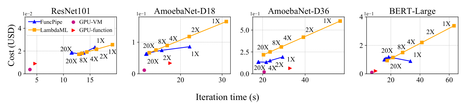
As our breakdown analysis in §5.3 shows that the improvement achieved by FuncPipe mostly comes from the reduced communication time, we are interested in the performance of FuncPipe when the network bandwidth increases. We simulate the performance of FuncPipe with the performance model proposed in §3.4 by changing the value of bandwidth . We compare the performance with that of the best-performing baseline LambdaML, which is simulated using its analytical model (Jiang et al. 2021). Fig. 11 reports the training speed and cost as we gradually increase the bandwidth to 20x of the current function bandwidth in AWS Lambda, i.e., from about 0.5 Gb/s to 10 Gb/s, which is a common bandwidth for a VM.
Generally, as the bandwidth increases, the performances of FuncPipe and LambdaML improve. The performance improvement of LambdaML is larger than that of FuncPipe as LambdaML has a higher communication cost. The relatively mild performance improvement of FuncPipe with the increase of bandwidth suggests that FuncPipe is more robust to different network settings. With 20X the bandwidth, compared with LambdaML, FuncPipe achieves comparable performances on ResNet101 and BERT-Large, i.e., 12.2% higher speed but 7.0% higher cost when training ResNet101, 12.9% higher speed but 6.3% higher cost when training BERT-Large. The trade-offs in speed and cost are caused by the small differences in the tendencies of the policies of FuncPipe and LambdaML. When training AmoebaNet-D18/AmoebaNet-D36, FuncPipe improves the training speed by 6.8%/14.0% while reducing the cost by 6.4%/38.6%. Such improvements are mostly attributed to FuncPipe’s optimized function memory allocation. This shows that even with the communication bottleneck removed, the memory allocation policy of FuncPipe can still benefit serverless-based training, although by a smaller margin.
Despite the improvements that FuncPipe achieves over existing serverless-based frameworks, a performance gap still exists between training with FuncPipe and GPU-enabled VM instances due to the lack of GPU support in serverless function. We conduct preliminary comparison by training the models on a popular p3.2xlarge AWS instance (equipped with a V100 GPU). As none of the models can be trained on the single GPU without causing memory overflow, we adopt gradient accumulation to reduce the memory consumption. The micro-batch size used for gradient accumulation is 4, the same as the micro-batch size in FuncPipe. The results reported in Fig. 11 show that GPU-based training can greatly outperform serverless CPU-based training in terms of cost, i.e. up to 90% cost reduction. The cause is that the per data sample processing cost of a vCPU can be tens of times higher than that of a GPU. Fortunately, some of the serverless platforms, e.g. Alibaba Cloud, are recently equipping their serverless functions with GPU (Alibaba 2022b). Similarly, we report the performance of training with a single serverless GPU function in Fig. 11. Note that as GPU function has yet not been made fully available to users, we evaluate the training speed on a GPU of the same type as the GPU function and obtain the cost with the announced GPU function price. The results show that GPU function greatly narrows gap in the per data sample processing cost with VM GPU instance. It is our next step of work to extend FuncPipe to such GPU function, evaluate its distributed training performance against VM GPUs and explore further optimization.
6. Related Work
Pipeline in serverless-based training. Dorylus (Thorpe et al. 2021) is a pipelined framework with a hybrid structure, i.e., CPU servers with serverless functions, for training Graph Neural Network (GNN) models. It exploits the inherent features of GNN to separate the computation tasks and uses serverless functions only for lightweight linear algebra operations. In contrast, our work exploits a serverless-based pipeline for training DNN models, which cannot be easily separated and trained the same way using Dorylus because they require much heavier computation and communication. Hydrozoa (Guo et al. 2022) proposes a pipelined framework that enables distributed training on GPU-enabled container instances. As serverless function has more stringent resource limits than container instance, our work focuses on providing more efficient communication design and careful co-optimization of model partition and resource allocation to tackle such resource challenges. Note that our optimization designs have the potential to benefit distributed training in other environments like the GPU-enabled container instances, as our preliminary experiments have demonstrated the benefits of our co-optimized model partition and resource allocation policy in GPU-based training.
Serverless communication. Feng et al. propose two centralized storage-based methods for model synchronization (Feng et al. 2018). However, such a design is generally of low efficiency due to the bandwidth bottleneck of the central nodes. LambdaML proposes a more efficient decentralized scatter-reduce method, but it fails to utilize the available bandwidth fully (Jiang et al. 2021). In parallel, other works focus on improving the performance of storage systems for higher communication efficiency. Pocket proposes a distributed data store that provides better elasticity and latency (Klimovic et al. 2018b). Shredder designs a low-latency cloud store that supports in-storage computing (Zhang et al. 2019). This line of work could be integrated with our pipelined storage-based communication approach to improving the network performance potentially. Another choice is to use common NAT-traversal techniques to enable direct communication among functions (Fouladi et al. 2019; Wawrzoniak and Bruno 2021). Direct communication can allow existing communication algorithms, e.g., ringAllreduce (Research 2017), to be used. However, NAT-traversal usually requires external servers that can cause communication bottlenecks. The performance of using existing communication designs for serverless-based training with NAT-traversal remains unclear.
Model partition and resource allocation in serverless. Recent works have studied the model partition and resource allocation problem for serverless-based inference serving (Yu et al. 2021; Jarachanthan et al. 2021). These works aim at satisfying Service Level Objectives in latency while minimizing cost or further improving throughput. Gillis fixes the per-function memory allocation and optimizes model partition to lower inference cost with a reinforcement learning approach (Yu et al. 2021). AMPS fixes the number of functions/partitions and co-optimizes the partition and memory allocation with a MIP formulation (Jarachanthan et al. 2021). Compared with inference, the optimization for distributed training, which is the focus of this work, includes more decision factors such as inner-stage data parallelism and synchronization cost and makes it more challenging to generate efficient model partition and resource configuration.
7. Conclusion
In this paper, we presented the design and implementation of a novel pipelined serverless training framework called FuncPipe. With the ever increasing interests in truly taking advantage of serverless computing, many researchers have looked at utilizing serverless functions to build scalable applications and improving serverless platforms (Wang et al. 2020b; Romero et al. 2021b; Romero et al. 2021a; Thorpe et al. 2021). Our key goal can be simply boiled down to understand how to allow DL practitioners to train models on serverless platforms in a fast and low-cost manner, regardless of model size and training hyperparameters such as batch size that impact memory consumption. With three key designs—(i) the pipeline parallelism for model partitions, (ii) the communication-efficient scatter-reduce, and (iii) the co-optimization of partition and resource allocation policy, FuncPipe was able to overcome the memory and bandwidth limitations of serverless platforms. We demonstrated the benefits of FuncPipe, i.e. 1.3X-2.2X training speedup and 7%-77% cost reduction compared to state-of-the-art serverless training frameworks (Jiang et al. 2021), by testing with four commonly used models and on two popular serverless providers in numerous settings. Interestingly, we observed that the benefits of FuncPipe remain even if the bandwidth of serverless functions increases to a level comparable to today’s VM bandwidth. This observation suggests the relevance of FuncPipe techniques even as the cloud providers continue to improve serverless infrastructure.
Acknowledgements.
This work was supported in part by the National Natural Science Foundation of China (No. 42050105, 62072302, 62020106005, 62061146002, 61960206002), the Program of Shanghai Academic/Technology Research Leader under Grant No. 18XD1401800, the US National Science Foundation under Grant NGSDI-2105564, and VMWare. We thank our shepherd Michael Ferdman, and the anonymous reviewers.References
- (1)
- Akkus et al. (2018) Istemi Ekin Akkus, Ruichuan Chen, Ivica Rimac, Manuel Stein, Klaus Satzke, Andre Beck, Paarijaat Aditya, and Volker Hilt. 2018. SAND: Towards High-Performance Serverless Computing. In 2018 Usenix Annual Technical Conference (USENIX ATC 18). 923–935.
- Alibaba (2022a) Alibaba. 2022a. Alibaba Cloud Function Compute. https://www.aliyun.com/product/fc.
- Alibaba (2022b) Alibaba. 2022b. Alibaba Cloud Function Compute Instance Type. https://help.aliyun.com/document_detail/179379.html.
- Alibaba (2022c) Alibaba. 2022c. Alibaba Cloud Object Storage Service. https://www.aliyun.com/product/oss.
- Alipourfard et al. (2017) Omid Alipourfard, Hongqiang Harry Liu, Jianshu Chen, Shivaram Venkataraman, Minlan Yu, and Ming Zhang. 2017. CherryPick: Adaptively Unearthing the Best Cloud Configurations for Big Data Analytics. In 14th USENIX Symposium on Networked Systems Design and Implementation (NSDI 17). 469–482.
- Amazon (2022) Amazon. 2022. AWS Lambda. https://www.aliyun.com/product/fc.
- Awan et al. (2020) Ammar Ahmad Awan, Arpan Jain, Quentin Anthony, Hari Subramoni, and Dhabaleswar K Panda. 2020. HyPar-Flow: exploiting MPI and Keras for scalable hybrid-parallel DNN training with tensorflow. In International Conference on High Performance Computing. 83–103.
- Bian et al. (2021) Zhengda Bian, Qifan Xu, Boxiang Wang, and Yang You. 2021. Maximizing Parallelism in Distributed Training for Huge Neural Networks. arXiv preprint arXiv:2105.14450 (2021).
- Bojja Venkatakrishnan et al. (2019) Shaileshh Bojja Venkatakrishnan, Shreyan Gupta, Hongzi Mao, Mohammad Alizadeh, et al. 2019. Learning Generalizable Device Placement Algorithms for Distributed Machine Learning. Advances in Neural Information Processing Systems 32 (2019).
- Brochu et al. (2010) Eric Brochu, Vlad M Cora, and Nando De Freitas. 2010. A tutorial on Bayesian optimization of expensive cost functions, with application to active user modeling and hierarchical reinforcement learning. arXiv preprint arXiv:1012.2599 (2010).
- Carreira et al. (2019) Joao Carreira, Pedro Fonseca, Alexey Tumanov, Andrew Zhang, and Randy Katz. 2019. Cirrus: A serverless framework for end-to-end ml workflows. In Proceedings of the ACM Symposium on Cloud Computing. 13–24.
- Chen et al. (2018) Chi-Chung Chen, Chia-Lin Yang, and Hsiang-Yun Cheng. 2018. Efficient and robust parallel dnn training through model parallelism on multi-gpu platform. arXiv preprint arXiv:1809.02839 (2018).
- Chu et al. (2020) Ching-Hsiang Chu, Pouya Kousha, Ammar Ahmad Awan, Kawthar Shafie Khorassani, Hari Subramoni, and Dhabaleswar K Panda. 2020. Nv-group: link-efficient reduction for distributed deep learning on modern dense gpu systems. In Proceedings of the 34th ACM International Conference on Supercomputing. 1–12.
- Devarakonda et al. (2017) Aditya Devarakonda, Maxim Naumov, and Michael Garland. 2017. Adabatch: Adaptive batch sizes for training deep neural networks. arXiv preprint arXiv:1712.02029 (2017).
- Domhan et al. (2015) Tobias Domhan, Jost Tobias Springenberg, and Frank Hutter. 2015. Speeding up automatic hyperparameter optimization of deep neural networks by extrapolation of learning curves. In Twenty-fourth international joint conference on artificial intelligence.
- Eismann et al. (2020) Simon Eismann, Joel Scheuner, Erwin Van Eyk, Maximilian Schwinger, Johannes Grohmann, Nikolas Herbst, Cristina L Abad, and Alexandru Iosup. 2020. Serverless applications: Why, when, and how? IEEE Software 38, 1 (2020), 32–39.
- Fan et al. (2021) Shiqing Fan, Yi Rong, Chen Meng, Zongyan Cao, Siyu Wang, Zhen Zheng, Chuan Wu, Guoping Long, Jun Yang, Lixue Xia, et al. 2021. DAPPLE: A pipelined data parallel approach for training large models. In Proceedings of the 26th ACM SIGPLAN Symposium on Principles and Practice of Parallel Programming. 431–445.
- Feng et al. (2018) Lang Feng, Prabhakar Kudva, Dilma Da Silva, and Jiang Hu. 2018. Exploring serverless computing for neural network training. In 2018 IEEE 11th international conference on cloud computing (CLOUD). IEEE, 334–341.
- Fouladi et al. (2019) Sadjad Fouladi, Francisco Romero, Dan Iter, Qian Li, Shuvo Chatterjee, Christos Kozyrakis, Matei Zaharia, and Keith Winstein. 2019. From laptop to lambda: Outsourcing everyday jobs to thousands of transient functional containers. In 2019 USENIX Annual Technical Conference (USENIX ATC 19). 475–488.
- Geng et al. (2019) Jinkun Geng, Dan Li, and Shuai Wang. 2019. Horizontal or vertical? a hybrid approach to large-scale distributed machine learning. In Proceedings of the 10th Workshop on Scientific Cloud Computing. 1–4.
- Guo et al. (2022) Runsheng Guo, Victor Guo, Antonio Kim, Josh Hildred, and Khuzaima Daudjee. 2022. Hydrozoa: Dynamic Hybrid-Parallel DNN Training on Serverless Containers. Proceedings of Machine Learning and Systems 4 (2022), 779–794.
- Gurobi (2022a) Gurobi. 2022a. Gurobi - The Fastest Solver. https://www.gurobi.com.
- Gurobi (2022b) Gurobi. 2022b. Setting up and using a Floating license. https://www.gurobi.com/documentation/9.5/quickstart_mac/setting_up_and_using_a_flo.html.
- Hafeez et al. (2021) Ubaid Ullah Hafeez, Xiao Sun, Anshul Gandhi, and Zhenhua Liu. 2021. Towards optimal placement and scheduling of DNN operations with Pesto. In Proceedings of the 22nd International Middleware Conference. 39–51.
- Hendrickson et al. (2016) Scott Hendrickson, Stephen Sturdevant, Tyler Harter, and Venkataramani. 2016. Serverless Computation with OpenLambda. In 8th USENIX Workshop on Hot Topics in Cloud Computing (HotCloud 16).
- Hu et al. (2021) Qinghao Hu, Peng Sun, Shengen Yan, Yonggang Wen, and Tianwei Zhang. 2021. Characterization and prediction of deep learning workloads in large-scale gpu datacenters. In Proceedings of the International Conference for High Performance Computing, Networking, Storage and Analysis. 1–15.
- Huang et al. (2019) Yanping Huang, Youlong Cheng, Ankur Bapna, Orhan Firat, Dehao Chen, Mia Chen, HyoukJoong Lee, Jiquan Ngiam, Quoc V Le, Yonghui Wu, et al. 2019. Gpipe: Efficient training of giant neural networks using pipeline parallelism. Advances in neural information processing systems 32 (2019).
- Jain et al. (2020a) Arpan Jain, Ammar Ahmad Awan, Asmaa M Aljuhani, Jahanzeb Maqbool Hashmi, Quentin G Anthony, Hari Subramoni, Dhableswar K Panda, Raghu Machiraju, and Anil Parwani. 2020a. Gems: Gpu-enabled memory-aware model-parallelism system for distributed dnn training. In SC20: International Conference for High Performance Computing, Networking, Storage and Analysis. IEEE, 1–15.
- Jain et al. (2020b) Arpan Jain, Ammar Ahmad Awan, Asmaa M Aljuhani, Jahanzeb Maqbool Hashmi, Quentin G Anthony, Hari Subramoni, Dhableswar K Panda, Raghu Machiraju, and Anil Parwani. 2020b. Gems: Gpu-enabled memory-aware model-parallelism system for distributed dnn training. In SC20: International Conference for High Performance Computing, Networking, Storage and Analysis. IEEE, 1–15.
- Jarachanthan et al. (2021) Jananie Jarachanthan, Li Chen, Fei Xu, and Bo Li. 2021. AMPS-Inf: Automatic Model Partitioning for Serverless Inference with Cost Efficiency. In 50th International Conference on Parallel Processing. 1–12.
- Jeon et al. (2020) Beomyeol Jeon, Linda Cai, Pallavi Srivastava, Jintao Jiang, Xiaolan Ke, Yitao Meng, Cong Xie, and Indranil Gupta. 2020. Baechi: fast device placement of machine learning graphs. In Proceedings of the 11th ACM Symposium on Cloud Computing. 416–430.
- Jeon et al. (2019) Myeongjae Jeon, Shivaram Venkataraman, Amar Phanishayee, Junjie Qian, Wencong Xiao, and Fan Yang. 2019. Analysis of Large-Scale Multi-Tenant GPU Clusters for DNN Training Workloads. In 2019 USENIX Annual Technical Conference (USENIX ATC 19). 947–960.
- Jia et al. (2018) Zhihao Jia, Sina Lin, Charles R. Qi, and Alex Aiken. 2018. Exploring Hidden Dimensions in Parallelizing Convolutional Neural Networks. In Proceedings of the 35th International Conference on Machine Learning, Vol. 80. 2279–2288.
- Jia et al. (2019) Zhihao Jia, Matei Zaharia, and Alex Aiken. 2019. Beyond Data and Model Parallelism for Deep Neural Networks. Proceedings of Machine Learning and Systems 1 (2019), 1–13.
- Jiang et al. (2021) Jiawei Jiang, Shaoduo Gan, Yue Liu, Fanlin Wang, Gustavo Alonso, Ana Klimovic, Ankit Singla, Wentao Wu, and Ce Zhang. 2021. Towards demystifying serverless machine learning training. In Proceedings of the 2021 International Conference on Management of Data. 857–871.
- Klimovic et al. (2018a) Ana Klimovic, Yawen Wang, Christos Kozyrakis, Patrick Stuedi, Jonas Pfefferle, and Animesh Trivedi. 2018a. Understanding ephemeral storage for serverless analytics. In 2018 USENIX Annual Technical Conference (USENIX ATC 18). 789–794.
- Klimovic et al. (2018b) Ana Klimovic, Yawen Wang, Patrick Stuedi, Animesh Trivedi, Jonas Pfefferle, and Christos Kozyrakis. 2018b. Pocket: Elastic ephemeral storage for serverless analytics. In 13th USENIX Symposium on Operating Systems Design and Implementation (OSDI 18). 427–444.
- Li et al. (2020a) Liam Li, Kevin Jamieson, Afshin Rostamizadeh, Ekaterina Gonina, Jonathan Ben-tzur, Moritz Hardt, Benjamin Recht, and Ameet Talwalkar. 2020a. A System for Massively Parallel Hyperparameter Tuning. In Proceedings of Machine Learning and Systems, Vol. 2. 230–246.
- Li and Hoefler (2021) Shigang Li and Torsten Hoefler. 2021. Chimera: efficiently training large-scale neural networks with bidirectional pipelines. In Proceedings of the International Conference for High Performance Computing, Networking, Storage and Analysis. 1–14.
- Li et al. (2021) Shijian Li, Oren Mangoubi, Lijie Xu, and Tian Guo. 2021. Sync-Switch: Hybrid Parameter Synchronization for Distributed Deep Learning. In 2021 IEEE 41th International Conference on Distributed Computing Systems (ICDCS).
- Li et al. (2020b) Shijian Li, Robert J. Walls, and Tian Guo. 2020b. Characterizing and Modeling Distributed Training with Transient Cloud GPU Servers. In 2020 IEEE 40th International Conference on Distributed Computing Systems (ICDCS).
- Li et al. (2020c) Shen Li, Yanli Zhao, Rohan Varma, Omkar Salpekar, Pieter Noordhuis, Teng Li, Adam Paszke, Jeff Smith, Brian Vaughan, Pritam Damania, and Soumith Chintala. 2020c. PyTorch Distributed: Experiences on Accelerating Data Parallel Training. Proc. VLDB Endow. 13, 12 (2020), 3005–3018.
- McDonald et al. (2010) Ryan McDonald, Keith Hall, and Gideon Mann. 2010. Distributed training strategies for the structured perceptron. In Human language technologies: The 2010 annual conference of the North American chapter of the association for computational linguistics. 456–464.
- McGrath and Brenner (2017) Garrett McGrath and Paul R Brenner. 2017. Serverless computing: Design, implementation, and performance. In 2017 IEEE 37th International Conference on Distributed Computing Systems Workshops (ICDCSW). IEEE, 405–410.
- Microsoft (2022a) Microsoft. 2022a. Microsoft Azure Cloud Computing. https://azure.microsoft.com/.
- Microsoft (2022b) Microsoft. 2022b. Microsoft Azure Storage. https://azure.microsoft.com/services/storage.
- Mirhoseini et al. (2018) Azalia Mirhoseini, Anna Goldie, Hieu Pham, Benoit Steiner, Quoc V. Le, and Jeff Dean. 2018. Hierarchical Planning for Device Placement. In ICLR.
- Mirhoseini et al. (2017) Azalia Mirhoseini, Hieu Pham, Quoc V Le, Benoit Steiner, Rasmus Larsen, Yuefeng Zhou, Naveen Kumar, Mohammad Norouzi, Samy Bengio, and Jeff Dean. 2017. Device placement optimization with reinforcement learning. In International Conference on Machine Learning. PMLR, 2430–2439.
- Narayanan et al. (2019) Deepak Narayanan, Aaron Harlap, Amar Phanishayee, Vivek Seshadri, Nikhil R Devanur, Gregory R Ganger, Phillip B Gibbons, and Matei Zaharia. 2019. PipeDream: generalized pipeline parallelism for DNN training. In Proceedings of the 27th ACM Symposium on Operating Systems Principles. 1–15.
- Narayanan et al. (2021) Deepak Narayanan, Mohammad Shoeybi, Jared Casper, Patrick LeGresley, Mostofa Patwary, Vijay Korthikanti, Dmitri Vainbrand, Prethvi Kashinkunti, Julie Bernauer, Bryan Catanzaro, Amar Phanishayee, and Matei Zaharia. 2021. Efficient Large-Scale Language Model Training on GPU Clusters Using Megatron-LM. In Proceedings of the International Conference for High Performance Computing, Networking, Storage and Analysis.
- Ngatchou et al. (2005) Patrick Ngatchou, Anahita Zarei, and A El-Sharkawi. 2005. Pareto multi objective optimization. In Proceedings of the 13th International Conference on, Intelligent Systems Application to Power Systems. IEEE, 84–91.
- Patarasuk and Yuan (2007) Pitch Patarasuk and Xin Yuan. 2007. Bandwidth efficient all-reduce operation on tree topologies. In 2007 IEEE International Parallel and Distributed Processing Symposium. IEEE, 1–8.
- Patarasuk and Yuan (2009) Pitch Patarasuk and Xin Yuan. 2009. Bandwidth optimal all-reduce algorithms for clusters of workstations. J. Parallel and Distrib. Comput. 69, 2 (2009), 117–124.
- Rausch et al. (2019) Thomas Rausch, Waldemar Hummer, Vinod Muthusamy, Alexander Rashed, and Schahram Dustdar. 2019. Towards a serverless platform for edge AI. In 2nd USENIX Workshop on Hot Topics in Edge Computing (HotEdge 19).
- Research (2017) Baidu Research. 2017. baidu-allreduce. https://github.com/baidu-research/baidu-allreduce.
- Romero et al. (2021a) Francisco Romero, Gohar Irfan Chaudhry, Íñigo Goiri, Pragna Gopa, Paul Batum, Neeraja J Yadwadkar, Rodrigo Fonseca, Christos Kozyrakis, and Ricardo Bianchini. 2021a. Faa$T: A Transparent Auto-Scaling Cache for Serverless Applications. (2021).
- Romero et al. (2021b) Francisco Romero, Mark Zhao, Neeraja J. Yadwadkar, and Christos Kozyrakis. 2021b. Llama: A Heterogeneous & Serverless Framework for Auto-Tuning Video Analytics Pipelines. In Proceedings of the ACM Symposium on Cloud Computing (Seattle, WA, USA) (SoCC’21).
- Shallue et al. (2019) Christopher J. Shallue, Jaehoon Lee, Joseph Antognini, Jascha Sohl-Dickstein, Roy Frostig, and George E. Dahl. 2019. Measuring the Effects of Data Parallelism on Neural Network Training. Journal of Machine Learning Research 20, 112 (2019), 1–49.
- Shazeer et al. (2018) Noam Shazeer, Youlong Cheng, Niki Parmar, Dustin Tran, Ashish Vaswani, Penporn Koanantakool, Peter Hawkins, et al. 2018. Mesh-tensorflow: Deep learning for supercomputers. Advances in neural information processing systems 31 (2018).
- Shoeybi et al. (2019) Mohammad Shoeybi, Mostofa Patwary, Raul Puri, Patrick LeGresley, Jared Casper, and Bryan Catanzaro. 2019. Megatron-lm: Training multi-billion parameter language models using model parallelism. arXiv preprint arXiv:1909.08053 (2019).
- Sohoni et al. (2019) Nimit Sharad Sohoni, Christopher Richard Aberger, Megan Leszczynski, Jian Zhang, and Christopher Ré. 2019. Low-memory neural network training: A technical report. arXiv preprint arXiv:1904.10631 (2019).
- Song et al. (2020) Liuyihan Song, Pan Pan, Kang Zhao, Hao Yang, Yiming Chen, Yingya Zhang, Yinghui Xu, and Rong Jin. 2020. Large-scale training system for 100-million classification at alibaba. In Proceedings of the 26th ACM SIGKDD International Conference on Knowledge Discovery & Data Mining. 2909–2930.
- Tarnawski et al. (2020) Jakub M Tarnawski, Amar Phanishayee, Nikhil Devanur, Divya Mahajan, and Fanny Nina Paravecino. 2020. Efficient algorithms for device placement of dnn graph operators. Advances in Neural Information Processing Systems 33 (2020), 15451–15463.
- Thakur et al. (2005) Rajeev Thakur, Rolf Rabenseifner, and William Gropp. 2005. Optimization of collective communication operations in MPICH. The International Journal of High Performance Computing Applications 19, 1 (2005), 49–66.
- Thorpe et al. (2021) John Thorpe, Yifan Qiao, Jonathan Eyolfson, Shen Teng, Guanzhou Hu, Zhihao Jia, Jinliang Wei, Keval Vora, Ravi Netravali, Miryung Kim, et al. 2021. Dorylus: Affordable, Scalable, and Accurate GNN Training with Distributed CPU Servers and Serverless Threads. In 15th USENIX Symposium on Operating Systems Design and Implementation (OSDI 21). 495–514.
- Vahidinia et al. (2020) Parichehr Vahidinia, Bahar Farahani, and Fereidoon Shams Aliee. 2020. Cold start in serverless computing: Current trends and mitigation strategies. In 2020 International Conference on Omni-layer Intelligent Systems (COINS). IEEE, 1–7.
- Wang et al. (2020b) Ao Wang, Jingyuan Zhang, Xiaolong Ma, Ali Anwar, Lukas Rupprecht, Dimitrios Skourtis, Vasily Tarasov, Feng Yan, and Yue Cheng. 2020b. InfiniCache: Exploiting Ephemeral Serverless Functions to Build a Cost-Effective Memory Cache. In 18th USENIX Conference on File and Storage Technologies (FAST 20). usenix.org, 267–281.
- Wang et al. (2019) Hao Wang, Di Niu, and Baochun Li. 2019. Distributed machine learning with a serverless architecture. In IEEE INFOCOM 2019-IEEE Conference on Computer Communications. IEEE, 1288–1296.
- Wang et al. (2020a) Linnan Wang, Rodrigo Fonseca, and Yuandong Tian. 2020a. Learning Search Space Partition for Black-box Optimization using Monte Carlo Tree Search. In Advances in Neural Information Processing Systems (NeurIPS), 2020 (online).
- Wang et al. (2018) Liang Wang, Mengyuan Li, Yinqian Zhang, Thomas Ristenpart, and Michael Swift. 2018. Peeking behind the curtains of serverless platforms. In 2018 USENIX Annual Technical Conference (USENIX ATC 18). 133–146.
- Wawrzoniak and Bruno (2021) Ingo Wawrzoniak, Mike and Fraga Barcelos Paulus Bruno. 2021. Boxer: Data Analytics on Network-enabled Serverless Platforms. In 11th Annual Conference on Innovative Data Systems Research.
- Xu et al. (2021) Fei Xu, Yiling Qin, Li Chen, Zhi Zhou, and Fangming Liu. 2021. DNN: Achieving Predictable Distributed DNN Training With Serverless Architectures. IEEE Trans. Comput. 71, 2 (2021), 450–463.
- Yu et al. (2021) Minchen Yu, Zhifeng Jiang, et al. 2021. Gillis: Serving Large Neural Networks in Serverless Functions with Automatic Model Partitioning. In 2021 IEEE 41st International Conference on Distributed Computing Systems (ICDCS). IEEE, 138–148.
- Zhang et al. (2019) Tian Zhang, Dong Xie, Feifei Li, and Ryan Stutsman. 2019. Narrowing the gap between serverless and its state with storage functions. In Proceedings of the ACM Symposium on Cloud Computing. 1–12.
- Zhang et al. (2016) Wei Zhang, Suyog Gupta, Xiangru Lian, and Ji Liu. 2016. Staleness-Aware Async-SGD for Distributed Deep Learning. In Proceedings of the Twenty-Fifth International Joint Conference on Artificial Intelligence (IJCAI’16). 2350–2356.
- Zhang et al. (2020) Zhen Zhang, Chaokun Chang, Haibin Lin, Yida Wang, Raman Arora, and Xin Jin. 2020. Is network the bottleneck of distributed training?. In Proceedings of the Workshop on Network Meets AI & ML. 8–13.
- Zhao et al. (2022) Yiyang Zhao, Linnan Wang, Kevin Yang, Tianjun Zhang, Tian Guo, and Yuandong Tian. 2022. Multi-objective Optimization by Learning Space Partitions. 10th International Conference on Learning Representations, ICLR (2022).
Appendix A Notations in §3.4
| Notation | Definition |
| basic memory consumption of a serverless worker | |
| total number of micro-batches | |
| number of model layers. | |
| unit price of serverless function | |
| latency from serverless worker to cloud storage | |
| model size of layer | |
| size of activations of layer per micro-batch | |
| size of output of layer per micro-batch | |
| size of gradients from layer to layer per micro-batch | |
| slowdown factor for computation due to resource contention | |
| number of data parallelism options | |
| value of -th data parallelism option | |
| number of resource allocation options | |
| memory size of -th resource option | |
| bandwidth of -th resource option | |
| forward computation time of layer with -th resource option | |
| backward computation time of layer with -th resource option | |
| , means model is partitioned between layers and | |
| , means the -th data parallelism option is chosen | |
| , means layer workers have -th memory size | |
| iteration time | |
| iteration cost | |
| forward time for full forward pipeline | |
| time for one micro-batch traverse forward pipeline | |
| lag between micro-batches at end of forward pipeline | |
| backward time until layer completes computation | |
| model synchronizing time at layer | |
| time for layer to upload its output to storage. | |
| time for layer to download input from storage. | |
| time for to upload gradient output to storage. | |
| time for layer to be download gradient from storage. | |
| degree of data parallelism, | |
| number of micro-batches per worker, | |
| memory size of layer worker, | |
| bandwidth of layer worker, | |
| accumulated activation size at layer (accumulated forwardly). | |
| accumulated model size at layer (accumulated forwardly). | |
| accumulated model size at layer (accumulated backwardly). | |
| accumulated forward computation time at layer (accumulated forwardly). | |
| accumulated backward computation time at layer (accumulated backwardly). |
Appendix B Backward Time
The backward computation time of layer , the upload and download time , between layers and are given by
where is the gradient size from layer to layer . We introduce a tilde operator similar to the hat operator in (4), except that it accumulates the quantities backwardly. The cumulative backward computation time from the previous partition boundary down to layer is given by
| (10) |
For each , define
| (11) |
where
When is the lowest layer of a partition, is the computation completion time of that partition, and is the corresponding lag between consecutive micro-batches. Note that if and layers and belong to the same partition.
Appendix C Linearization
First we present the major linearization techniques used to convert the non-linear binary integer programming to MIQP:
Technique 1: Linearizing the multiplication of two binary variables. , can be linearized as follows:
Technique 2: Linearizing the multiplication of a continuous variable and a binary variable. , is a continuous variable, can be linearized as follows:
Technique 3: Linearizing of the operator. are continuous variables, can be linearized as follows:
where is a large constant. Next we introduce how we linearize the formulation in detail.
- (1)
Linearizing the equality constraint for the cumulative values , , , and . We introduce , , , and as continuous variables and linearize their equality constraints. We use in (10) as an example and it is similar with the others. We can write as:
Since is a binary variable, can be converted to a new binary variable by recursively performing linearization with Technique 1. Then continuous variable satisfies the following constraint
and are both binary variables, thus can be linearized applying Technique 1.
- (2)
Linearizing the equality constraint for , , and . We introduce , , and as continuous variables and linearize their equality constraints. We use as an example and it is similar with the others. We can write in (8) as:
and are both binary variables, thus can be linearized applying Technique 1.
- (3)
Linearizing forward time and backward time . We use as an example and it is similar with . Linearizing in (11) is equal to linearizing . Since is the of a set of continuous variables, it can be presented as a continuous variable with linear constraints using Technique 3. Expand , we have
Since is a continuous variable and is a binary variable, can be linearized applying Technique 2.
- (4)
Linearizing . Expand (9), we have
and are binary variables, is a continuous variable, thus we can first linearize using Technique 2 and then further linearize by applying Technique 2 again.
- (5)
Linearizing full iteration time . So far we have linearized , and in (7). We can further remove the operator using Technique 3.
- (6)
Linearizing total memory allocation . Expand (5), we have
Since , , and are all binary variables, and can be linearized using Technique 1.
- (7)
Linearizing memory constraint. At last, we linearize the memory constraint, the first constraint in (3). Expand the constraint, we have
and can both be linearized with Technique 2.
Appendix D A FuncPipe function example
Below is a code example for training with FuncPipe. As highlighted in orange, only minimal changes to the Pytorch training code are required.
Appendix E Performance Model Accuracy
Table 3 displays the prediction error in training time for the measured points of FuncPipe in Fig. 5. The results show that our performance model achieves an average prediction error of less than 12%. The largest error happens when training Amoebanet-D36 with a global batch size of . We note that this error is mainly caused by the unexpected bandwidth variation; other model training is less impacted as they use fewer serverless workers and are less subject to the performance interference among workers. We leave the consideration of such interference in our performance model as part of future work.
| 16 | 64 | 256 | Average | |
| ResNet101 | 5.9% | 11.2% | 15.4% | 10.8% |
| Amoebanet-D18 | 13.3% | 9.0% | 10.6% | 11.0% |
| Amoebanet-D36 | 10.8% | 4.0% | 18.1% | 11.0% |
| Bert-large | 9.8% | 11.0% | 16.4% | 12.4% |
| Average | 9.9% | 8.8% | 15.1% | 11.3% |