98.80.-k, 96.25.De, 96.90.+c
Local dynamical effects of scale invariance: the lunar recession
Abstract
Scale invariance is expected in empty Universe models, while the presence of matter tends to suppress it.
As shown recently, scale invariance is certainly absent in cosmological models with densities
equal to or above the critical value .
For models with densities below ,
the possibility of limited effects remains open.
If present, scale invariance would be a global cosmological
property. Some traces could be observable locally. For the Earth-Moon two-body system, the predicted additional lunar recession
would be increased by 0.92 cm/yr, while the tidal interaction would also be slightly increased.
The Earth-Moon distance is the most systematically measured distance in the Solar System, thanks to
the Lunar Laser Ranging (LLR) experiment active since 1970.
The observed lunar recession from LLR amounts to 3.83 () cm/yr;
implying a tidal change of the length-of-the-day (LOD) by 2.395 ms/cy. However, the observed change of the LOD
since the Babylonian Antiquity is only 1.78 ms/cy, a result supported by paleontological data, and
implying a lunar recession of 2.85 cm/yr.
The significant difference of (3.83-2.85) cm/yr = 0.98 cm/yr,
already pointed out by several authors over the last two decades,
corresponds well to the predictions of the scale-invariant theory,
which is also supported by several other astrophysical tests.
keywords
cosmology, dark energy, Earth-Moon system1 Introduction
The scale-invariant theory aims at responding to a most fundamental principle expressed by Dirac [11]: “It appears as one of the fundamental principles in Nature that the equations expressing basic laws should be invariant under the widest possible group of transformations”. Our objective is to explore whether, in addition to Galilean invariance, Lorentz invariance, and general covariance, some effects of scale invariance would also be present in our low density Universe. This is particularly justified since scale invariance is present in Maxwell’s equations in absence of charges and currents, while in General Relativity (GR) scale invariance is a property of the empty space in absence of a cosmological constant, a property pointed out by [4].
Clearly, the presence of matter tends to kill scale invariance as shown by [17]. Thus, the question arises about how much matter in the Universe is necessary for suppressing scale invariance. Would one single atom in the Universe be enough to kill scale invariance? Clearly, we do not know whether this is the case, but the way to get an answer to the above questions is to carefully examine the theoretical consequences of this assumption and to perform comparisons with observations. From the scale covariant expressions of the Ricci tensor, curvature scalar and general field equation developped by [11] and [7], cosmological models were obtained by [23] who showed that scale invariance is clearly forbidden for models with matter densities equal and above the critical density . This result was found consistent with considerations [30] on causal connexion in Universe models.
These models also indicate that, as soon that one considers models with a density parameter , scale-invariant effects are drastically reduced, before totally disappearing at . For a Universe model with , they are nevertheless sufficient to drive a significant acceleration of the expansion. Several positive results have been obtained, e.g. on the distance modulus vs. reshifts relation, the Hubble rate vs. age and density parameter, the vs. relations, even if due to the observed scatter the discrimination from the CDM is difficult at present [23], [28]. The growth of density fluctuations is accounted for without the need of dark matter [27]; the same for the observed mass excess in clusters of galaxies [24]; and the radial acceleration relation for galaxies is reproduced [29]. For a brief summery of the Scale Invariant Vacuum paradigm and its main results and current progress see [20].
The question whether astrophysical systems, such as the solar system and galaxies, follow the Hubble-Lemaître expansion has stimulated a vast literature since the pioneer work of McVittie [33, 34] and the Einstein-Straus theorem [16]. The presence of an expansion at smaller scales has been considered as an open question by Bonnor [5] and recently revisited by us [31]. The fact that the dark-energy dominates the matter-energy content of the Universe and that this energy appears as driving the acceleration of expansion is reviving the interest in the question: If dark energy is uniformly distributed in space would it not imply effects that may be present at small scales? The Earth-Moon system occupies a particular place in this context, since there are direct accurate measurements of the evolution of the distance in this two-body system.
It is thus appropriate to examine whether there are some local effects of scale invariance, e.g. in the Solar System. According to several pioneer works [26, 14, 15, 22] the local effects in the Solar System due to scale invariance would have been of the order of the Hubble-Lemaître expansion or some fraction of it. (The Hubble-Lemaître expansion with km s-1 Mpc-1 corresponds to 10.7 m/yr for one astronomical unit, or 2.75 cm/yr for the Earth-Moon distance of 384’400 km). For the proper interpretation of these effects in the scale-invariant context, it is necessary to account for the limitations of the -variations due to a significant matter density in the Universe, and this implies a refined analysis, which we do here.
Section 2 briefly recalls the main points of the scale-invariant vacuum idea. Section 3 examines the limitations of the scale-factor and their impact on timescales. In Section 4, we study the weak-field low-velocity approximation of the scale-invariant field equation and the two-body problem. In Section 5, we compare the predicted and observed lunar recession from Lunar Laser Ranging (LLR) in relation with the data on the length-of-the day (LOD). Section 6 gives the conclusions.
2 Some points on the scale invariant vacuum (SIV) theory
Some recalls on the scale-invariant framework have been given recently [30], with references therein. In short, the theory is expressed in the cotensor framework appropriate to the Integrable Weyl Geometry developed by [11] and [7]. The developpements are rather parallel to those of General Relativity (GR), but with the possibility of conformal scale transformations of the form,
| (1) |
in addition to the general covariance. Primed quantities refer to the GR framework, while quantities without a prime refer to the scale covariant context. Scale covariant first and second derivatives, scale covariant Christoffel symbols, Riemann-Christoffel cotensor, Ricci cotensor and total co-curvature have been developed in the Integrable Weyl Geometry by [11], leading to a general scale covariant field equation [7].
In GR, one needs to define the line element corresponding to the physical system studied, for example the FLWR line element is adopted for expressing the cosmological equations in a homogeneous and isotropic Universe. Similarly, in the scale covariant context, an additional condition is necessary to fix the gauge. Dirac and Canuto et al. had chosen the then in vogue “Large Number Hypothesis“ [12]. We prefer to adopt as basic gauging condition the following assumption: The macroscopic empty space is scale invariant, homogeneous and isotropic. This is a simple and most reasonable assumption, which is consistent with the scale invariance of the equations of Maxwell and of General Relativity in empty space, as recalled in the introduction. Moreover, the equation of state of the vacuum is precisely the one equation permitting the vacuum density to remain constant for an adiabatic expansion or contraction [9]. We also note that the assumption of homogeneity and isotropy appears a reasonnable one for the macroscopic empty space.
Within the cotensor framework, our gauging condition can be expressed as follows [23],
| (2) |
It is what is left from the scale covariant field equation if space is empty 11 1 The de Sitter metric for empty space with is conformal to the Minkowski metric, and is identical to it for the condition . This condition is consistent with the solution (7. The first member (LHS) results from the scale invariant form of the Ricci tensor [11]. The second member (RHS) contains only the cosmological constant in the scale covariant form, with
| (3) |
is the cosmological constant in GR. The first member of Eq.(2) contains terms depending on , the coefficient of metrical connection, related to the scale factor of Eq. (1),
| (4) |
We note that if the scale factor is a constant, all terms in vanish and Eq. (2) implies . This means that the scale-invariant field equation just becomes the field equation of GR without a cosmological constant.
For reasons of homogeneity and isotropy of the empty space, the scale factor should depend on time only, so that the only non-zero component of is ,
| (5) |
In Weyl’s Integrable Geometry, is playing a fundamental role alike the . From the time and space components of Equation (2) one obtains:
| (6) |
Thus, the gauging conditions leads to analytical relations between the scale factor and the cosmological constant, which represents the energy density of the vacuum. These differential equations give a new physical significance to the cosmological constant, which now appears as the energy density of the relative variations of the scale factor, see the first of Eqs.(6) and [30] for its connection to inflationary stage of the very early Universe. The solution of these differential equations is
| (7) |
We take the present time and also consider the present scale as a reference to which all scales are referred to. Thus, may be written as,
| (8) |
Remarkably, the gauging condition, which implies the two equations (6), lead to major simplifications of the cosmological equations derived by [7] on the basis of the general field equations. One obtains [23]:
| (9) | |||
| (10) |
On the right side of both, we note an additional term. For a constant , Friedmann’s equations are recovered. A third equation may be derived from the above two,
| (11) |
Since is negative, the extra term represents an additional acceleration in the direction of the motion. Thus, the effects of the scale invariance are fundamentally different from those of a cosmological constant. For an expanding Universe, this extra force produces an accelerated expansion, without requiring dark energy. For a contraction, the additional term favors collapse. This is exactly what the corresponding term in the weak-field approximation is also doing, as verified in the study of the growth of density fluctuations [27]. There, the additional term favors contraction and allows an early formation of galaxies in absence of dark matter.
3 Limits on the variations of the scale factor
3.1 Solutions of the cosmological equations for
Analytical solutions for the flat scale-invariant models with have been obtained by [21] in the case of matter dominated models, with the corresponding equation of conservation,
| (12) |
It is noticeable that an analytical solution exists. It is expressed in the timescale where at present and . Such solutions are illustrated in [23] and [30]. Along with with as usual. There is no meaningful scale-invariant solution for equal or larger than 1, consistently with causality relations [30]. We see that the initial time when , the Big Bang, is at:
| (13) |
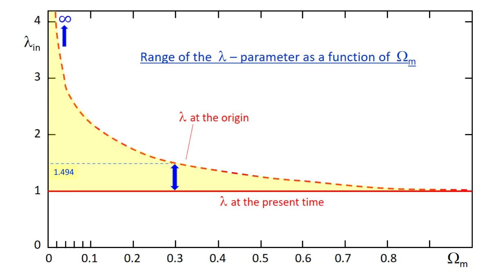
This dependence in 1/3 produces a rapid increase of for increasing low matter density. For , the values of are 0, 0.215, 0.464, 0.669, 0.794. Since , this leads to a strong reduction of the range of -variations for increasing matter densities as illustrated in Fig. 1. While the range of scale variations is infinite between the Big Bang and now for an empty Universe model, the range would be very limited for significant -values, for example from only 1.494 to 1.0 for The Hubble parameter, in the same timescale, is
| (14) |
Thus, varies between and the infinite for between 0 and 1. We also write
| (15) |
These are respectively the normalized contributions (vs. ) of the matter, space curvature, and scale factor . With these definitions equation (9) leads to,
| (16) |
These quantities are usually considered at the present time. In the case of energy-density dominated by radiation and relativistic matter, for flat scale-invariant models with , analytical solutions for the expansion factor, the matter density, the radiation density and temperature have been obtained by [25].
3.2 Some essential properties of the scale-invariant solutions
Let us further examine the conditions of applicability of the above results:
- 1.
Case of for homogeneous and isotropic Einstein-like empty space, but not necessarily empty Universe with homogeneous and isotropic cosmological space. The two equations (6) and their solution (7) for have been derived for the macroscopic empty space, under the assumption that it is homogeneous and isotropic, which implies a dependence of on time only. The empty space obeys an equation and in the scale-invariant theory the vacuum density is also related to the cosmological constant by . For one has and and the cosmological equation (11) then implies , which is the trace of the matter energy-momentum tensor.
Alike in GR, the properties of the vacuum and thus of the cosmological constant are intrinsic characteristics of the vacuum space, not depending on any matter content and distribution, and so was it also in the derivation of Eqs. (6). Thus, these equations and their solution apply everywhere in the Universe, independently of . As a consequence, the solution is a universal function, characteristic of the empty space. Let us note that the energy density of the empty space can be expressed in term of a scalar field ,
| (17) |
with the constant . The field obeys a modified Klein-Gordon equation and is advantageously playing the role of the “inflaton” during inflation [30].
- 2.
Case of in presence of matter. The presence of matter could be viewed as space inhomogeneities below certain scale but absent at larger scales and especially at cosmic scales. The presence of matter is determined by the density parameter , which influences the interval of time between the initial time and . For a higher -value (between 0 and 1), the interval is smaller and so does the range of the -values. In this indirect way, the presence of matter drastically reduces the range of variation of the scale factor (Fig. 1). Most importantly, we easily verify that in the scale-invariant context (Section 3.1), does not change during the evolution of the Universe, both in the matter and radiation eras. As long as the radiation era is very short and negligible compared to the full age of the Universe, then the initial time defines as a constant for the Universe.
Thus, steps 1 and 2 show that the function has a form which is universal , but the range of the time variations, and thus of , is strongly limited by the matter content.
- 3.
Case of for comoving galaxies. Now, comouving galaxies have the same timescale and thus the same age (the cosmic time). Thus, the parameter, its first, second derivatives and the coefficient of metrical connection are the same in all comoving galaxies:
(18)
Therefore, we are led to the following global conclusion: The universal function and its limitations apply the same way in all comouving galaxies. Thus, the effects of the variations of with their limitations could also be expected locally, e.g. in the Solar System, which is a low velocity subpart of a comoving galaxy.
3.3 Relations between timescales
We have two different timescales (both concerning the cosmic time): (1.) The age of the above cosmological model, with at the present time and at the origin. (2.) The usual timescale , with Gyr at the present time [18] and at the Big-Bang. The relation between ages in the two timescales is,
| (19) |
This means that for an event at a given epoch, the age fraction with respect to the present age is the same in both timescales. This gives the two following relations between particular times and ,
| (20) |
For the derivatives of these two timescales, we have,
| (21) |
These derivatives have constant values, implying that the two times are linearly connected. For larger -values, is also larger (13) and the timescale is squeezed over a smaller fraction of the interval [0,1] as [, ]. The above expressions are useful to express the relative variations of the scale factor as function of ages.
4 The dynamical equation and the two-body problem
4.1 The weak-field low-velocity approximation of the equation of motion
This approximation in the scale-invariant framework is leading to a modified expression of the Newton’s Law [26, 24]. In spherical coordinates, it is
| (22) |
This expression for a weak field is derived from the geodesic equation by Dirac in the reference [11], which was also obtained from an action principle by [6]. The conservation law for a dust Universe in the scale invariant context imposes a relation of the form [23]: This means that the inertial mass of a particle or of an object is not necessarily a constant, a situation which also occurs in GR and Special Relativity where the inertial mass of an object depends on its velocity. Within SIV the mass is evolving like in the same way as the length, so that, interestingly enough, the gravitational potential of an object is a scale-invariant quantity. We call the mass that varies like , where is the cosmic time. In a Universe model with , a mass at the present time was at time , at the Big-Bang. Over small and moderate time intervals, the mass may often be considered as a constant.
With respect to the classical expression, there is an additional acceleration term in the direction of motion. This term proportional to the velocity is favoring collapse in an accretion system and favoring expansion in a two-body system. From here onwards, we call the gravitational constant (a true constant), expressed in the appropriate units in the above cosmological models, while wil now on be reserved to the value expressed in the current time units (years, seconds).
Equation (22) contains terms and derivatives which are functions of the universal , the range of which is squeezed by the limited range of the adopted -scale in the cosmological models. As increases, a given range in the current time units (e.g. 2 Gyr) is expressed in terms of the corresponding smaller interval. We need to convert the equation of motion (22) expressed with variable into terms of the cosmic time in the current units (years, seconds) with an origin at and a present value Gyr. Equation (22) becomes,
| (23) |
The corresponding units of in the usual -scale are . Thus, we have the correspondence with the usual units conversion. At the present epoch or in the current units, the masses and are evidently equal. At other epochs, the relation is,
| (24) |
This results in the correct scaling of expected mass at the Big Bang to be compared with ; therefore, .
Thus, multiplying both members of Eq.(23) by , we get at time ,
| (25) |
We see that the presence of matter () always reduces the effect of the additional acceleration term, for it disappears. Now, let us consider the situation at the present time . We define the numerical factor using:
| (26) |
The modified Newton’s equation at present time , currently 13.8 Gyr, is then:
| (27) |
The small additional term depends on the global cosmology, in particular on parameter , as discussed above. In an empty Universe, . For , one has . For higher values, consistently with the discussion of the Eq. (12) the additional term would be absent [30]. In the case with , one has . Thus, the additional acceleration term is significantly reduced.
4.2 The two-body problem with -limitations
Let us now consider a two-body system within the SIV theory with and a density parameter . From Eq.(22) in the -scale, the orbital motion was found to be still described by the Binet equation (the mass change being accounted for) and thus obeying the equation of conics [26] and [24]
| (28) |
The parameter is related to the semi-major axis , semi-minor axis , and eccentricity via the relationships:
| (29) |
The eccentricity is a scale-invariant quantity. For , one has a circular orbit with a radius . There is a small growth of the parameter , or for as we consider here, first in the time -scale,
| (30) |
Thus, the orbital motion of a bound system is described by a circle (or an ellipse) with a slight superposed outwards spiraling motion. Quite interestingly, the small cosmological expansion keeps the orbital velocity constant. This reminiscent of the behaviour in MOND, where the speed on an orbit becomes asymptotically independent of the size of the orbit [35].
The above expressions formally only apply within an empty Universe with The limitations of the range of - and -variations given by Eqs. (20) are not yet included. Clearly, we have to account for them in a Universe with a density parameter different from zero. Thus, with Eqs. (20) and (21) we may write the relative change of the orbital radius (or parameter ),
| (31) |
This applies at a time . Let us consider, at the present epoch where the orbital radius is , an interval of time (say one year) very small with respect to Gyr. We may thus write the relative change of the orbital distance during this small interval of time,
| (32) |
For , we would get and thus . In a Universe model with a density parameter , the temporal increase of the orbital parameter is smaller than that in an empty universe (). For tending to 1, the relative orbital increase tends to zero. For , the factor is equal to 0.4152, 0.3306, 0.2632 respectively. Below, we will consider the standard model with . On the whole, the account of matter strongly reduces the expected effects of scale invariance.
5 Study of the Earth-Moon system
5.1 The LLR data
Let us turn to the observations. Since March 1970, the Earth-Moon distance has been intensively measured by Lunar Laser Ranging (LLR), first at Mc Donald Observatory and since the 80’s at several other observatories around the world. A total of 20’138 ranges up to September 2015 have been performed leading to an average lunar recession of 3.83 cm/yr [43, 44]. We note the impressive accuracy. The value of the lunar recession has not much changed since the first determination more than three decades ago [8], which illustrates the quality of the measurements. The Earth-Moon distance is the most intensively and systematically measured distance in the Solar System and the only one by a direct laser signal.
The main effect producing this recession is the Earth-Moon tidal coupling: the tidal bump of the Earth embarked by the fast Earth axial rotation, with an angular velocity faster than that of the Moon on its orbits, generates a forward pull on the Moon. This pull is transferring some axial terrestrial angular momentum to the lunar orbital one. Over geological times, the lunar recession has likely changed since the Moon was closer to the Earth and thus the tidal exchanges were larger. For example, a lunar recession of about 6.5 cm/yr was estimated for the Ediacaran - Early Cambrian period (about 600 Myr ago) by [1].
5.2 The LOD data
According to the theoretical modeling of the tidal waves, lunar motion, and terrestrial rotation by [43], the observed lunar recession of 3.83 cm/yr implies an increase of the length of the day (LOD) of 2.395 ms/cy (millisecond per century). The LOD is defined as the excess of the length of the day with respect to 86’400 SI seconds. We note that the value of 2.395 ms/yr for the change of the LOD over centuries is consistent with the calculation of the tidal coupling under the assumption of conservation of the global angular momentum of the Earth-Moon system [14, 31]. This theoretical value of the increase of the LOD has also been very well confirmed recently by [2]. These authors revisited the Earth rotation theories with a two-layer deformable Earth model, including dissipative effects at the core-mantle boundary and account of the coupling torque between the two. The deceleration is numerically estimated with frequency-dependent modeling of the various solid and oceanic tides. In the assumption of the long-term coupling of the core and mantle, they obtain a deceleration of the Earth rotation corresponding to an increase of the LOD of 2.418 ms/cy in very good agreement with the above modeling by [43].
The best and longest studies on the change of the LOD in History have been performed by Stephenson et al. [40], who analyzed the lunar and solar eclipses from 720 BC up to 1600 AD and found an average shift of the LOD by 1.78 ( 0.03) ms/cy. Such a shift, apparently very small, is acting every day and progressively produces large effects over a long period. When cumulated over 2000 yr, differences in the time of solar and lunar eclipses are amounting to about 18’000 s. Such time differences are leading to big shifts in the eclipse locations, up to thousands of km. The constraints on the eclipse locations and indications (when available) about the time of the eclipse allowed Stephenson et al. to make the above determination, which had only slightly changed in their successive papers since 1984, see references in [40]. These authors also suggested the existence of a slight undulation around the mean with a period of 1500 yr, possibly related to the effect of magnetic core-envelope coupling [13].
Various other effects may contribute to the LOD, with different timescales: atmospheric effects, ice melting and change of the sea level, glacial isostatic adjustment, and core-envelope coupling. The most uncertain contribution is that of the core coupling which seems responsible for the 1500 yr undulation. Over the long term, the various negative and positive effects appear to balance each other before the year 1990, see data by [36, 37] and our recent detailed review of the problem [31], (since 1990, the fast melting of even the polar ice fields contribute to an increase of the Earth momentum of inertia). The reality of the difference between the above observed mean value of the LOD (1.78 ms/cy) and the value due to the tidal interaction (2.395 ms/cy) has recently been further emphasized by [41].
We note that other estimates of the change of the LOD have been made from lunar occultations, however on a shorter time basis. The observations of lunar occultations from 1656 to 1986 have been analyzed by [32], they indicate a slowing down of the Earth of 0.73 () ms/cy. The data show some decadal variations around the mean, which were also present in the further analyses. Various astronomical telescopic observations over the last 350 yr were analyzed by [39], which led to a mean increase of the LOD of 0.9 ms/cy. A new determination of the change of the LOD based on the data from [40] for occultations since 1680 complemented by IERS data for the period 1970 to 2020 has been performed recently by us [31]. We showed an average increase of 1.09 () ms/cy for the LOD over that period. All these determinations based on relatively limited durations are more subject to decadal fluctuations than the ancient eclipse observations.
Interestingly enough, another independent very long-term determination of the deceleration of the Earth rotation has been established on the basis of paleontological studies by Deines and Williams [10]. These authors examined all available paleontological fossils and deposits for direct measurements of Earth’s rotation, in particular they used corals, bivalves, brachipods, rythmites and stromatolites. These fossils are keeping the traces of phases of daily growth due to the alternance of days and nights. The oldest records go back to 1.85 Gyr ago, however such very ancient data are highly uncertain. Much more reliable data are availablle since the Cambrian explosion of the forms of life, when animals with hard shells first appeared, about 542 Myr ago. From their whole sample, [10] found a clear decrease of the number of days in one year. For example, 400 Myr ago, an epoch where there are lots of data, the mean number of days in one year (considered of constant duration, but see below) was about days (with an uncertainty of about 7 days). From their sample of collected data, Deines and Williams found a mean deceleration corresponding to a change of the LOD 1.642 ( 0.48) ms/cy. This mean value is quite interesting, although not taken at present time it concerns an age differing by less 3% of the present age of the Universe. The error is larger than the one by Stephenson et al. [40] ( ms/cy). Nevertheless, it gives another value consistent with and independent of the value by Stephenson et al. [40]. Based on an incredibly much longer time period, the result by Deines and Williams is supporting the discrepancy between the change of the LOD and the value of the lunar recession.
5.3 Theoretical Predictions of the two-body problem
Let us consider the possible increase of the Earth-Moon distance during one year in the scale-invariant context. For an empty Universe with an age of Gyr and a mean Earth-Moon distance of km, the lunar recession would be
| (33) |
This is close to the Hubble-Lemaître expansion rate with km/(s Mpc), corresponding to a lunar recession of 2.75 . For a Universe with , and the predicted cosmological expansion of the Earth-Moon system is,
| (34) |
a value substantially smaller than the Hubble-Lemaître expansion.
Let us also shortly consider the Earth-Mars distance. The relevant parameters are:
Mars : km, , km.
Earth: km, , km.
The difference of parameters for Mars and the Earth is km. The estimate of the Mars-Earth recession based on this distance would be in an empty Universe, With the factor for , we get
| (35) |
5.4 The tidal interaction in the scale invariant context
Let us also examine the tidal interaction in the Earth-Moon system. The law of angular momentum conservation for a given mass element in the scale invariant framework [26], is , while both and , are scaling like , e.g. . Let us examine the conservation of the total angular momentum of the Earth (E)–Moon (M) system at time [14],
| (36) |
The angle is the variable angle between the lunar orbital plane and the Earth equator. The numerical factor accounts for the consequences of the eccentricity of the lunar orbit, see numerical value below. Quantities and are respectively the moment of inertia and the axial angular velocity of the Earth. is the mass of the Moon and its orbital angular velocity. is the mean distance between the Earth and Moon. is the total angular momentum at the present time . We neglect the axial angular momentum of the Moon, since its mass is 1.2 % of that of the Earth and its axial rotation period (equal to its orbital period) is 27.3 days. Thus, the lunar axial angular momentum is a fraction of about of that of the Earth.
Let us evaluate the time derivative of the above expression (36),
| (37) |
Account has been given to the change of the moment of inertia due to the mass variation. is the axial rotation period of the Earth. For , we have the relation , which also applies in the SIV context, there is the Earth’s mass. We can develop the third term on the left of the above expression (37),
| (38) |
Indeed, as well as . Introducing this expression in Eq.(37) and explicating the time dependence of the various terms leads to
| (39) |
From this relation, we now extract the lunar recession , which becomes after some simplifications,
| (40) |
We may write it in a more condensed form by defining a constant ,
| (41) |
By using (since is scaling like equation (40) can now be written as:
| (42) |
For a time differing very little from , e.g. by one year, one has , and thus with a high accuracy we write,
| (43) |
The first term on the right represents the tidal effect linking the change of the LOD and the lunar recession, the second term results from the increase of the moment of inertia of the Earth (which reduces the lunar recession), the third term expresses the global expansion of the system. Interestingly enough, this third term is just the same as that predicted by the study of to the two-body problem, which shows the internal consistency of both approaches. We note that the change of the mass of the Moon is also contained in this third term, it was intervening through the last term in Eq.(40).
We have now to bring the above equation in the current time units, seconds and years. With Eq. (20) and (21), we get
| (44) |
In a cosmological Universe model with , the ratio . The constant is here in the units of , while is in the units of . Thus, both have to be turned -units and the scaling factors simplify. Thus, and can finally be both expressed in current time units (seconds or years).
5.5 Numerical values and discussion
We adopt the following numerical values of the various astronomical quantities
| (45) | |||
The value 0.331 is obtained from precession data [42]. Coefficient . The angle varies between 18.16 and 28.72 degrees, thus we adopt a mean value of . We have to estimate the value of . The tidal effects behave like , thus they depend on the eccentricity like . The time spent in an interval of angles goes like , thus like . The product of the two leads to a dependence of the form . For , let us take a value of which leads to . We thus obtain for the coefficient cm s-1.
Let us evaluate numerically the various contributions. With the LOD of 1.78 ms/cy from the antique data by [40], the first term contributes to a lunar recession of 2.85 cm/yr, while the LOD of 1.09 ms/cy from 1680 to the present [31] leads to a recession of 1.74 cm/yr. The second term in Eq. (44) gives for the case of ,
| (46) |
The direct expansion effect is
| (47) |
This term corresponds to a third of the general Hubble-Lemaitre expansion. Summing the various contributions, we get
| (48) |
Thus, we see that the scale invariant analysis is giving a relatively good agreement with the lunar recession of 3.83 cm/yr obtained from LLR observations. The difference amounts only to 10 % of the observed lunar recession. This is clearly much better than in the standard case, where the predicted LOD of 2.395 ms/cy corresponding to the observed recession diverges from the observed one of 1.78 ms/cy by 35 %. Thus, the scale invariant analysis appears to give more consistent results that the standard case. We do not consider this as a proof of the scale invariant theory, but this shows that the SIV theory deserves some attention, especially since more than several other astrophysical tests (see introduction) are successful.
We point out that the discrepancy between the observed LOD from historical records and the observed lunar recession has already been mentioned by several authors. Munk [38] has emphasized the interest of the discrepancy between the LLR lunar recession and the LOD data, invoking climatic effects. However, this would not be consistent with the data by Deines and Williams [10] which cover a much longer period of time over the geological epochs. Dumin [14] has also clearly demonstrated the above discrepancy between the LLR and the LOD results, showing that there was an excess of lunar recession of about 1.3 cm/yr not accounted by the slowing down of the Earth, an excess which would correspond to a fraction of about the half of the Hubble expansion. Dumin further studied this discrepancy and discussed some possible origins of it [15]. Krizek and Somer [22] have supported a local expansion of at least the order of the half of Hubble rate from an analysis of various properties in the Solar System. Also, the reality of the discrepancy between the observed LOD and the lunar recession was emphasized by Stephenson et al. [41].
On one side, we may of course wonder whether this small effect of about 1.3 cm/yr is sufficient to claim for an additional symmetry property in Physics. On the other side, steps forward often come by scrutinizing minute differences. Also, a larger effect would have already been found by more people than the few above precursors.
6 Conclusions
We have studied several mechanical properties in the scale invariant context, in particular we have shown the large reduction of the additional dynamical effects with the matter density. We have considered the two-body problem and the tidal interaction in the Earth-Moon system. As examples in the two-body system, independently of tidal effects, there would be a cosmological increase of 0.92 cm/yr for the Earth-Moon distance.
The observed lunar recession from LLR data amounts to 3.83 () cm/yr and the corresponding theoretical tidal change of the LOD is 2.395 ms/cy [43, 44]. Now, the observed change of the LOD since the Babylonian Antiquity is only 1.78 ms/cy, leading to a significant difference of 35 % [41]. Moreover, the value of 1.78 ms/cy is supported by the data from paleontology over hundreds million years. Such a change of the LOD would correspond to a lunar recession of 2.85 cm/yr, instead of 3.83 cm/yr as observed. The difference in the lunar recession is well accounted for within the dynamics of the SIV theory (48). A minima, the above results shows that the problem of scale invariance is worth of some attention.
7 Acknowledgments:
A.M. expresses his gratitude to his wife for her patience and support. V.G. is extremely grateful to his wife and daughters for their understanding and family support during the various stages of the research presented. This research did not receive any specific grant from funding agencies in the public, commercial, or not-for-profit sectors.
8 APPENDIX: A note on the result of Banik and Kroupa
A criticism of the scale invariant theory was expressed by Banik and Kroupa [3] with the argument that “the predicted expansion of the Earth–Moon orbit is incompatible with lunar laser ranging data at ”. They used the following expression for the change of the lunar angular velocity,
| (49) |
The correct expression in the scale invariant theory (SIV) is according to the unmodified expression of the orbital velocity , and thus via one has:
| (50) |
Now, is given by Eq.(44), where the first term on the right of this equation corresponds to in (49),
| (51) |
The first and last terms on the right simplify, we get
| (52) |
The first two terms are identical with those of Banik and Kroupa, however the last term, which is an important one, is absent in their equation. This clearly invalidate their claim. On the contrary, the results of the present work confirm the remarkable compatibility of the scale invariant theory with the observed lunar recession, an agreement which does not exist in the standard theory.
References
- [1] Azarevich, M.B., Lopez, V.L.: Lunar recession encoded in tidal rhythmites: a selective overview with examples from Argentina Geo-Marine Letters. 37 (2017),333–344
- [2] Baenas, T., Escapa, A., Ferrandiz, J.M.: Secular changes in length of day: Effect of the mass redistribution Astron. & Astrophys.648 (2021), 89–98
- [3] Banik, I., Kroupa, P.: Scale invariant dynamics in the Solar system. MNRAS, 407 (2020), L62-66
- [4] Bondi, H.: The cosmological scene 1945-1952. Modern Cosmology in Retrospect (1990) Bertotti, B., Balbinot, R., & Bergia, S. Cambridge Univ. Press., 189
- [5] Bonnor, W.B. Local Dynamics and the Expansion of the Universe. Gen. Rel. Grav. 32 (2000) 1005.
- [6] Bouvier, P., Maeder, A.: Consistency of Weyl’s Geometry as a Framework for Gravitation. Astroph. Space Sci. 54 (1978), 497-508
- [7] Canuto, V., Adams, P. J., Hsieh, S.-H., & Tsiang, E.: Scale-covariant theory of gravitation and astrophysical applications. Phys. Rev.D. 16 (1977), 1643-1663
- [8] Christodoulidis, D. C., Smith, D. E., Williamson, R. G. et al.: Observed Tidal Braking in the Earth/moon/sun System. J. Geophys. Res. 93(B6) (1988), 6216–6236
- [9] Carroll, S. M., Press, W. H., & Turner, E. L.: The Cosmological Constant. Ann. Eev. Astron. Astrphys. 30, 499–542
- [10] Deines, S.D., Williams, C.A.: Earth’s rotational deceleration: determination of tidal friction independent of timescales. Astron.Journal. 151 (2016). 103–114
- [11] Dirac, P. A. M.: Long range forces and broken symmetries, Proceedings of the Royal Society of London Series A, 333 (1973), 403–418
- [12] Dirac, P. A. M.: Cosmological Models and the Large Numbers Hypothesis. Proceedings of the Royal Society of London Series A, 338 (1974), 439–446
- [13] Dumberry, M, Bloxham, J.: Azimuthal flows in the Earth’s core and changes in length of day at millennial timescales. Geophys. Journal. 165 (2006), 32–46
- [14] Dumin, Yu.V.: A new application of the lunar laser retroreflectors: Searching for the “local” hubble expansion. Adv. Space Res. 31 (2003), 2461-2466
- [15] Dumin, Yu.V.: Local Hubble expansion: current state of the problem. In Cosmology on Small Scales (2016), Eds. M. Krizek and Y. Dumin, Institute of Math. CAS, Prague, 23–40
- [16] Einstein, A., Straus, E.G.: The Influence of the Expansion of Space on the Gravitation Fields Surrounding the Individual Stars. Rev. Mod. Phys. 17 (1945), 120.
- [17] Feynman, R. P.: Mainly mechanics, radiation, and heat. Feynman lectures on physics, 1(1963)
- [18] Frieman, J. A., Turner, M. S., & Huterer, D.: Dark energy and the accelerating universe. Ann. Rev. Astron. Astrophys. 46 (2008), 385–437
- [19] Gross, R.: Earth Rotation Variations - Long period, in Treatise of Geophysics, vol 3, Geodesy (2009) Ed. G. Schubert, Elsevier, Amsterdam, p. 239
- [20] Gueorguiev, V.G.; Maeder, A. The Scale Invariant Vacuum Paradigm: Main Results and Current Progress. Universe 8 (2022) 213.
- [21] Jesus, J.F. : Exact solution for flat scale-invariant cosmology. Rev. Mex. Astron. Astrophys. 55 (2018), 17–20
- [22] Krizek, M., Somer, L.: Anthropic principleand the local Hubble expansion. In Cosmology on Small Scales (2016), Eds. M. Krizek and Y. Dumin, Institute of Math. CAS, Prague, 65–94
- [23] Maeder, A.: An Alternative to the LambdaCDM Model: The Case of Scale Invariance. Astrophys. J. 834 (2017a), 194–210
- [24] Maeder, A.: Dynamical Effects of the Scale Invariance of the Empty Space: The Fall of Dark Matter? Astrophys. J. 849 (2017c),158–177
- [25] Maeder, A.: Evolution of the early Universe in the scale-invariant theory. arXiv:1902.10115.
- [26] Maeder, A., Bouvier, P.: Scale invariance, Metrical Connection and the Motions of Astronomical Bodies. Astron. Astrophys., 73 (1979), 82-89
- [27] Maeder, A.; Gueorguiev, V.G.: The growth of the density fluctuations in the scale-invariant vacuum theory Physics of the Dark Universe, 25 (2019), 100315–100330
- [28] Maeder, A.; Gueorguiev, V.G.: The Scale-Invariant Vacuum (SIV) Theory: A Possible Origin of Dark Matter and Dark Energy. Universe, 6 (2020a), 46
- [29] Maeder, A.; Gueorguiev, V.G. Scale-invariant dynamics of galaxies, MOND, dark matter, and the dwarf spheroidals. MNRAS, 492(2020b), 2698
- [30] Maeder, A.; Gueorguiev, V.G.: Scale invariance, horizons, and inflation. MNRAS 504 (2021a), 4005-4014
- [31] Maeder, A.; Gueorguiev, V.G.: On the relation of the lunar recession and the length-of-the-day. Astroph. Space Sci. 366 (2021b), 101–125
- [32] McCarthy, D.D., Babcock, A.: The length of day since 1656. Physics of the Earth and Planetary Interiors. 44 (1986), 281–292
- [33] McVittie, G.C. Condensations in an Expanding Universe. MNRAS 92 (1932) 500.
- [34] McVittie, C.G. The Mass-Particle in an Expanding Universe. MNRAS 93 (1933) 325.
- [35] Milgrom, M.: MOND laws of galactic dynamics. MNRAS 437 (2014), 2531–2541
- [36] Mitrovica, J.X., Wahr, J.: Ice Age Earth Rotation. Ann. Rev. Earth & Planetary Sci. 39 2011), 577–616
- [37] Mitrovica, J.X., Hay, C.C., Morrow, E. et al.: Reconciling past changes in Earth’s rotation with 20th century global sea-level rise: Resolving Munk’s enigma Sci. Adv. 1 (2015), e1500679-1500684
- [38] Munk,W.H.: Twentieth century sea level: An enigma. Proc.Natl. Acad. Sci. USA. 99 (2002), 6550–6555.
- [39] Sidorenkov, N.S.: The effect of the El Nino Southern oscillation on the excitation of the Chandler motion of the Earth’s pole. Astron. Reports (in Russian). 41 (1997), 705–708
- [40] Stephenson, F.R., Morrison, L.V., Hohenkerk, C.Y.: Measurement of the Earth’s rotation: 720 BC to AD 2015. Proc. R. Soc. A472 (2016), 404–430.
- [41] Stephenson, F.R., Morrison, L.V., Hohenkerk, C.Y.: Eclipses and the Earth’s Rotation General Assembly,Proceedings of the IAU IAU XXX (2020), 160–162
- [42] Williams, J.G.: Contribution to the Earth’s Obliquity Rate, Precession, and Nutation Astron. J. 108 (1994), 71
- [43] Williams, J.G., Boggs, D.H., Ratcliff, J.T.: Lunar Tidal Recession. 47th Lunar and Planetary Science Conference (2016a), 1096-1100
- [44] Williams, J.G., Boggs, D.H.: Secular tidal changes in lunar orbit and Earth rotation. Celestial Mechanics and Dynamical Astron. 126 (2016b), 89–129