Anomaly Detection by Leveraging Incomplete Anomalous Knowledge with Anomaly-Aware Bidirectional GANs
Abstract
The goal of anomaly detection is to identify anomalous samples from normal ones. In this paper, a small number of anomalies are assumed to be available at the training stage, but they are assumed to be collected only from several anomaly types, leaving the majority of anomaly types not represented in the collected anomaly dataset at all. To effectively leverage this kind of incomplete anomalous knowledge represented by the collected anomalies, we propose to learn a probability distribution that can not only model the normal samples, but also guarantee to assign low density values for the collected anomalies. To this end, an anomaly-aware generative adversarial network (GAN) is developed, which, in addition to modeling the normal samples as most GANs do, is able to explicitly avoid assigning probabilities for collected anomalous samples. Moreover, to facilitate the computation of anomaly detection criteria like reconstruction error, the proposed anomaly-aware GAN is designed to be bidirectional, attaching an encoder for the generator. Extensive experimental results demonstrate that our proposed method is able to effectively make use of the incomplete anomalous information, leading to significant performance gains compared to existing methods11 1 Code is available at https://github.com/tbw162/AA-BiGAN..
1 Introduction
Anomaly detection aims to identify anomalous samples from normal ones, with applications widely found in fields ranging from network security Garcia-Teodoro et al. 2009, financial fraud detection Abdallah et al. 2016, industrial damage detection to medical diagnosis Fernando et al. 2021 etc. In anomaly detection, normal data generally refers to samples preserving some kinds of regularities (typically composed of one or several types of samples), while anomaly often lacks an explicit and clear definition. Generally, any samples that deviate significantly from the normal ones are considered as anomalies. Obviously, according to this definition, the types of anomalies are numerous and sometimes even infinite. The extreme diversity of anomalies distinguish the anomaly detection problem from other tasks and also poses a significant challenge to it.


Existing anomaly detection methods can be roughly grouped into supervised and unsupervised categories. By assuming a full accessibility to anomalies during the training, supervised methods turn the anomaly detection problem into a classification problem. Anomalous samples are generally more difficult and expensive to collect, thus unsupervised methods that only rely on the use of normal samples are used more widely in practice. Despite it is difficult to collect anomalies from every anomaly type, collecting anomalies from one or several types is often possible. For instance, by viewing images of skin diseases as anomalies, it is easy to collect some images of commonly observed skin diseases, but impossible to collect images for all known and unknown skin diseases. Under the circumstances with incompletely collected anomalies, we can still resort to the unsupervised methods by neglecting the anomalies already collected. But this approach will definitely not lead to the optimal performance for not leveraging the available anomalous knowledge, as illustrated in Fig. 1(a). Supervised methods, on the other hand, essentially seek to find a decision boundary that can separate the normal and collected anomalous samples. However, since the collected anomalies only represent a fraction of all anomaly types, when a anomaly of unseen type is presented, the classifier may not be able to classify it correctly, as illustrated in Fig. 1(b).
To leverage the incompletely collected anomalies, a semi-supervised anomaly detection method SSAD is proposed in Görnitz et al. 2013, which learns a compact hyper-sphere that encompasses the normal samples, while excluding the collected anomalies outside of it. In Deep SAD Ruff et al. 2019, a deep neural network is trained to encourage the learned representations of normal samples gathering towards a common center, while those of anomalies moving away from it, increasing the discrimination between normal and anomalous samples’ representations. Obviously, both methods are established on a good distance metric, which, however, is often very difficult to be found, especially in the high-dimensional data space like images. Recently, Das et al. 2020 proposed to incorporate the information of anomalies identified by an expert into a basic anomaly detector through active learning framework. However, the active learning approach requires the collected anomalies to be processed one by one, losing the merits of batch processing. Moreover, to integrate with the active learning, the basic anomaly detector used in Das et al. 2020 is relatively simple, making it not suitable to be used in high-dimensional data.
In this paper, we argue that the most natural way to address this problem is to approach it from the perspective of probabilistic distribution learning. Under this view, the problem can be reformulated as learning a distribution that can not only model the normal samples well, but also ensure low density values for the collected anomalies, as illustrated in Fig. 1(c). Inspired by recent successes of deep generative models Goodfellow et al. 2014, we propose to ground this problem on them. But different from previous generative models, we developed a generative model that can not only capture the distribution of samples from the normal dataset, but also avoid to assign probabilities for samples in the abnormal dataset. Specifically, an anomaly-aware generative adversarial network (GAN) is developed, which is able to explicitly avoid generating samples that look like the training anomalies, apart from the basic capability of generating normal samples. Moreover, due to the high computational cost of directly evaluating the density value, following the unsupervised anomaly detection methods based on GANs Zenati et al. 2018b, we make the proposed anomaly-aware GAN to be bidirectional, too. With the bidirectional structure, surrogate metrics (e.g., reconstruction error) can be easily calculated to assess the abnormality of a new sample. Extensive experiments were conducted to evaluate the performance of the proposed method. The results demonstrate that the proposed method is able to exploit the collected anomalies to boost the detection performance effectively, and outperforms the comparable baselines by a remarkable margin.
2 Preliminaries of GAN-Based Unsupervised Anomaly Detection
One of the main approach for unsupervised anomaly detection is to estimate the probability distribution of normal data. Generative adversarial networks (GANs) Goodfellow et al. 2014, known for their superior capability of modeling the distribution of high-dimensional data like images, have been applied to detect anomalies. In Schlegl et al. 2017, a vanilla GAN is trained to model the normal data by playing a min-max game
| (1) |
where and represent the generator and discriminator, respectively; and are the distribution of normal data and standard Gaussian distribution, respectively. After training, a joint distribution over the data and latent code is obtained. However, due to the prohibitive computational complexity involved in the integration , the density cannot be used to detect anomalies directly. Instead, Schlegl et al. 2017 proposed to use gradient descent methods to find a latent code that can explain the data in the latent space, and then use the reconstruction error between original data and the recovered data to assess the abnormality, that is, . Some other surrogate criteria are also proposed, e.g., leveraging the learned discriminator Zenati et al. 2018a; Sinha et al. 2020. Since the discriminator is not trained to distinguish anomalies from normal data, these criteria generally do not perform as well as the reconstruction error.
Bidirectional-GAN-Based Methods
To reduce the computational cost of searching the latent code, bidirectional GANs Dumoulin et al. 2017; Li et al. 2017; Donahue et al. 2017 were later used for anomaly detection, in which the associated encoder can output the latent codes directly. For a bidirectional GAN, it includes two joint distributions, the encoder-induced and generator-induced joint distribution
| (2) | ||||
| (3) |
where and represent the encoder and generator , respectively, both of which are parameterized by neural networks. It is proved in Dumoulin et al. 2017 that and will converge to the same distribution by playing the following min-max game
| (4) |
Since is defined as and holds after convergence, it can be easily seen that the marginal distribution of w.r.t. must be , and can be viewed as the inference network of . Thus, for a sample , we can use the inference network to output its latent code and then use to compute the reconstruction error.
3 Anomaly Detection with Anomaly-Aware Bidirectional GANs
3.1 Problem Description
To describe the problem clearly, we define two datasets
| (5) | ||||
| (6) |
where and denote the set of normal samples and collected anomalies, respectively. According to the characteristics of anomaly detection tasks, we assume that the normal population can be sufficiently represented by the dataset , while because of the extreme diversity of anomalies, only contain a fraction of anomaly types and cannot be used to represent the whole abnormal population. The problem interested in this paper is to judge a testing sample is anomalous or not based on the two given datasets and . Unsupervised detection methods only leverage the normal dataset , while supervised ones leverage both but assume that can represent the entire anomaly population. Both of the methods are not suitable for the considered circumstance. Note that the dataset is assumed to be only composed of normal samples in the analyses below, but we will show experimentally that it could be mixed with some anomalies, leading to only a slight performance drop.
3.2 Enabling Anomaly-Awareness for Bidirectional GANs under Disjoint Supports
Deep generative models have been successfully applied to detect anomalies by learning the distribution of normal samples in , but none of them make use of the collected anomalies in . In this section, to leverage the available anomalous information given by in , an Anomaly-Aware Bidirectional GAN (AA-BiGAN) is developed, which can explicitly avoid to assign probabilities for samples in . To this end, we first transform the traditional bidirectional GAN described in (2) into the framework of least-square GAN (LSGAN) Mao et al. 2017, which using least-square loss to realize the updating equations. It is known that the optimization objective (2) aims to drive the output of discriminator towards 1 and 0 for samples from and , respectively, while encouraging the generator and encoder to confuse the discriminator by driving it to output 0.5. Under the LSGAN framework, least-square loss is used to replace the cross-entropy loss in (2), leading to the following updating rules
| (7) |
| (8) |
where the generator and encoder refer to the conditional distribution and , respectively; and and . Following similar proofs in LSGAN, we can obtain the lemma.
Lemma 1.
Proof.
Please refer to the Supplementary Materials. ∎
Although it is known that the marginal of joint distribution is equal to the training data distribution after convergence, the method still lacks the ability of explicitly avoiding to assign probabilities for samples in . To achieve this goal, we modify the updating rules in (3.2) and (3.2) by adding an anomaly-relevant term
| (9) |
| (10) |
where the distributions
| (11) | ||||
| (12) |
and represent the distributions of samples in and , respectively. Although the exact expressions of and are not known, we can easily draw samples from them. The optimal discriminator is obtained
| (13) |
By substituting the optimal discriminator into (3.2), it can be easily verified that under the prerequisite of disjoint support , the optima is achieved if and only if . Therefore, we have the following theorem
Theorem 2.
Proof.
Please refer to Supplementary Materials. ∎
From Theorem 2, it can be seen that due to , the marginal of generative distribution will converge to , which is the same as previous GANs when is set as . Although the new updating rules do not change the converged distribution, they bring us a different optimal discriminator as shown in (13), which is aware of the distribution of collected anomalies. To see this, let us examine the training dynamics of the generator. Suppose that a sample is generated from the generative model . If the sample looks similar to the collected anomalies, that is, , according to the discriminator in (13), its output value must be very small i.e., close to . Since the target value of discriminator is 0.5 for the training of generator, the significant discrepancy between the two values will push the generator quickly moving away from current state. Therefore, the discriminator (13) is able to prevent the generator from generating anomaly-like samples. By contrast, it can be easily shown that when setting as , the optimal discriminator of previous GANs obtained by (2) or (3.2) and (3.2) is
| (14) |
which does not include the anomaly-relevant term in the discriminator. Without this term, even if a sample that looks similar to anomalies is generated, the discriminator is not guaranteed to output a small value. As a result, the discriminator in (14) does not have the capability of explicitly preventing the generator from generating anomaly-like samples. Although theoretically the marginal of both generative distributions, no matter which discriminator is used, will converge to eventually, this is established on the assumptions of infinite training data and infinite representational capacities of neural networks. However, none of these conditions can be satisfied in practice, making the learned distribution only be an approximate of the ideal distribution . Therefore, the collected anomalies are possibly assigned with some non-negligible probabilities in the learned distribution. However, if the anomaly-aware discriminator (13) is used, this kind of possibilities could be reduced significantly, thanks to the model’s capability of explicitly avoiding to generate anomaly-like samples.
3.3 Relaxing the Prerequisites
The derivation of anomaly-aware bidirectional GANs in the previous section hinges on the prerequisite of disjoint supports for distributions of normal and anomalous samples and , that is, . However, the disjoint condition may not always hold in practice, especially when the anomalies and normal samples share lots of commonalities. In this section, we show that this prerequisite can be removed by adjusting the target values of discriminator. Moreover, we can also show that the target values do not need to be restricted to some fixed values, but could have lots of feasible configurations. To be specific, we have the following theorem.
Theorem 3.
If the discriminator , generator and encoder are updated according to
| (15) |
| (16) |
the two distributions and after convergence will be equal, that is, .
Proof.
Please refer to the Supplementary Materials. ∎
The proof of this theorem relies on the use of Jensen inequality and is more complex than that of Theorem 2. According to this theorem, we are able to obtain a bidirectional generative model that can explicitly avoid to generate anomaly-like samples even if the disjoint supports condition does not hold. For the parameters , and , theoretically they could be set arbitrary. In the experiments, we follow LSGAN and set and as and , respectively. For the value of , we find that the performance is not sensitive to its value, as demonstrated by the results in Supplementary Materials. We observed that letting it far away from , and generally deliver a slightly better performance, thus we simply set it set as for all experiments.
3.4 Detection Methods
With the anomaly-aware bidirectional GAN, we can apply it to identify anomalies for new samples. Due to the difficulties of computing the marginal densities , reconstruction error is used as the surrogate criteria to replace the density value, as found in many generative-model based anomaly detection methods An and Cho 2015; Zenati et al. 2018b. Specifically, we employ the encoder to produce a latent code for the sample , and then use the generator to generate a sample from the code . The error is then used to indicate the degree of abnormality of input sample . It is widely observed that the vanilla bidirectional GANs do not reconstruct the input well. Thus, to increase their reconstruction ability, as proposed in Li et al. 2017, one more discriminator is added to distinguish the pairs between and , with the specific expression deferred to the Supplementary Materials. In addition to the reconstruction error, some papers Akcay et al. 2018 also proposed to use the norm of latent code to detect anomalies by noticing that the codes of normal samples follow a standard normal distribution . Thus, if a code’s norm is large, it is highly suspected of being an anomaly. In practice, we find that both of the two criteria work well, but show some differences on specific datasets. In our experiments, we simply choose the one with better performance on the validation subset for a specific dataset.
4 Related work
With the recent advancement of deep learning, neural networks have been used to help anomaly detection Pang et al. 2021a. Among the existing methods, a typical approach is to train a deep model to reconstruct the normal data and then employ the reconstruction error to detect anomalies Xia et al. 2015. To achieve better and robust performance, variational auto-encoders (VAE) Kingma and Welling 2014 are further used in An and Cho 2015. To increase the distinction between the reconstruction errors of normal and anomalous samples, a memory module Gong et al. 2019 and discriminators Perera et al. 2019 are added into the autoencoders. Another type of mainstream generative models, generative adversarial networks (GAN), are also widely used for anomaly detection Schlegl et al. 2017. To obtain the reconstruction error more cheaply, bidirectional GANs Dumoulin et al. 2017 are proposed to use in Zenati et al. 2018b. In addition to reconstruction-based methods, many methods established on density estimation are also studied, e.g., estimating the density distribution of normal samples using energy-based models Zhai et al. 2016 or deep Gaussian mixture models Zong et al. 2018, and then using the density value to detect anomalies. There are also many other methods that resort to the one-class classifier, which assumes that normal samples can often be encompassed by a compact hypersphere Tax and Duin 2004 or separated by a hyperplane Schölkopf et al. 2001. Deep SVDD Ruff et al. 2018 is further proposed, which uses neural networks to learn discriminative representations for normal and anomalous samples and then finds a hypersphere to separate them like SVDD. In recent years, it has been pointed out that it is possible to collect a handful of anomalies before the training in practice. Early methods simply turn this problem into a binary classification problem Kingma et al. 2014, without considering the incompleteness of the collected anomalies. Differently, SSAD Görnitz et al. 2013 proposed to ground the problem on unsupervised detection method SVDD, while ensuring the available anomalous samples are outside of the hypersphere. Later, deep SAD Ruff et al. 2019 proposed to learn a mapping function that encourages the representations of normal samples gathering toward a center, while those of collected anomalies moving away from it. Although both methods achieve superior performance, these methods heavily rely on the use of a good distance metric, which is often difficult to be found in high-dimensional data. Recently, Das et al. 2020 seeks to use active learning to incorporate the anomalies identified by an expert into the existing basic anomaly detector. Pang et al. 2021b proposed a reinforcement-learning-based method to actively seek novel types of anomalies. However, the architecture of basic anomaly detectors employed in both methods is relatively simple, impeding them from being applied to high-dimensional data with complex structure like images.
5 Experiments
5.1 Experimental Setups
Datasets
Following the setups in Deep SAD Ruff et al. 2019, we first evaluate the detection performance of our method on three image datasets. i) MNIST: A dataset consisting of 60000 training and 10000 testing handwritten digit images of 2828 from 10 classes. ii) F-MNIST: A dataset consisting of 60000 training and 10000 testing fashion images of 2828 from 10 classes. iii) CIFAR10: A dataset consisting of 50000 training and 10000 testing images from ten classes. Then, six classic anomaly detection datasets are used to further evaluate the performance of proposed method.
Training & Evaluation
Following the paper Ruff et al. 2019, for each dataset, we select one category as normal, while treating the remaining nine types as anomalies. To mimic the circumstance of incomplete anomalous information, a proportion of samples from one of the nine anomalous categories have been collected. The proposed model is trained on the normal samples and collected anomalies. The testing dataset is splitted into a validation and testing dataset with a ratio of and . The hyperparameters are fine-tuned on the validation dataset, please refer to the Supplementary Material for more details of training. The area under the receiver operating characteristic curve (AUROC) is employed as the performance criteria. The reported experimental results are averaged over 90 experiments (i.e., 10 choices of normal categories 9 choices of anomalous categories).
| Data | SSAD Raw | SSAD Hybrid | SS-DGM | Supervised Classifier | Deep SAD | NDA | AA-BiGAN (ours) | |
| .00 | 96.0 2.9 | 96.3 2.5 | n.a. | n.a. | 92.8 4.9 | 86.5 9.5 | 96.3 2.8 | |
| .01 | 96.6 2.4 | 96.8 2.3 | 89.9 9.2 | 92.8 5.5 | 96.4 2.7 | 96.5 3.7 | 97.4 2.1 | |
| MNIST | .05 | 93.3 3.6 | 97.4 2.0 | 92.2 5.6 | 94.5 4.6 | 96.7 2.4 | 96.8 3.2 | 97.8 2.0 |
| .10 | 90.7 4.4 | 97.6 1.7 | 91.6 5.5 | 95.0 4.7 | 96.9 2.3 | 96.9 3.0 | 98.4 1.7 | |
| .20 | 87.2 5.6 | 97.8 1.5 | 91.2 5.6 | 95.6 4.4 | 96.9 2.4 | 97.1 2.9 | 98.2 1.6 | |
| .00 | 92.8 4.7 | 91.2 4.7 | n.a. | n.a. | 89.2 6.2 | 82.7 11.4 | 93.0 4.8 | |
| .01 | 92.1 5.0 | 89.4 6.0 | 65.1 16.3 | 74.4 13.6 | 90.0 6.4 | 90.1 8.5 | 94.4 5.0 | |
| F-MNIST | .05 | 88.3 6.2 | 90.5 5.9 | 71.4 12.7 | 76.8 13.2 | 90.5 6.5 | 91.0 7.1 | 94.6 4.2 |
| .10 | 85.5 7.1 | 91.0 5.6 | 72.9 12.2 | 79.0 12.3 | 91.3 6.0 | 91.4 7.0 | 94.7 4.3 | |
| .20 | 82.0 8.0 | 89.7 6.6 | 74.7 13.5 | 81.4 12.0 | 91.0 5.5 | 91.4 7.1 | 94.8 4.1 | |
| .00 | 62.0 10.6 | 63.8 9.0 | n.a. | n.a. | 60.9 9.4 | 64.8 8.2 | 65.0 9.4 | |
| .01 | 73.0 8.0 | 70.5 8.3 | 49.7 1.7 | 55.6 5.0 | 72.6 7.4 | 73.4 7.7 | 80.2 6.6 | |
| CIFAR-10 | .05 | 71.5 8.1 | 73.3 8.4 | 50.8 4.7 | 63.5 8.0 | 77.9 7.2 | 78.9 7.7 | 81.5 6.4 |
| .10 | 70.1 8.1 | 74.0 8.1 | 52.0 5.5 | 67.7 9.6 | 79.8 7.1 | 80.1 7.6 | 83.6 6.4 | |
| .20 | 67.4 8.8 | 74.5 8.0 | 53.2 6.7 | 80.5 5.9 | 81.9 7.0 | 81.6 7.3 | 84.8 7.2 |
Baselines
Semi-supervised anomaly detection methods are used for comparison: SSAD Görnitz et al. 2013, SS-DGM Kingma et al. 2014, Deep SAD Ruff et al. 2019, negative data augmentation method (NDA) Sinha et al. 2020, and active anomaly detection (AAD) Das et al. 2020 for tabular dataset. In addition, a supervised binary classifier is also trained for comparison. The performance of these methods, except NDA and AAD, are quoted from Deep SAD in Ruff et al. 2019. The NDA and AAD papers concentrate on different scenarios as ours, thus we report their performance by running and tuning their publicized code on our experiments.
5.2 Performance and Analysis
Overall Performance
Table 1 shows the performance of our proposed model. To investigate how the number of collected anomalies affects the performance, the performance is evaluated under different values of , where is defined as the ratio between the number of collected anomalies and the number of normal samples. When is set to , the semi-supervised methods are reduced to the unsupervised ones. It can be seen that as long as a very small fraction of anomalies is used, a significant performance improvement can be observed, especially on the complex dataset of CIFAR-10. And as the ratio of available anomalies further increases, a steady improvement can be observed. Under the specific case of , the performance gains observed in our proposed method over the best baseline on MNIST, F-MNIST and CIFAR-10 are , and , respectively, demonstrating that our method can exploit the partially-observed anomalies effectively to boost the overall detection performance. Moreover, it can be also seen that as the dataset of interest becomes more complex, the advantages of our proposed method become more clear. This may be attributed to the strong ability of GANs in modeling the probabilistic distribution of image data. By contrast, due to the difficulties of finding an appropriate metric to measure the distance in high-dimensional data space, distance-based detection methods, like SSAD and Deep SAD, struggle in such scenarios. As for the NDA, although it is also established on GANs, it focuses more on the generation of images, lacking the necessary bidirectional structure to produce the surrogate detection criteria like reconstruction error as in our model.
Performance with polluted normal dataset
In some scenarios, it may be difficult to obtain a clean dataset , in which a small proportion of anomalous samples may be mixed. To investigate how our proposed model performs under such circumstances, experiments are conducted under different ratios of pollution , where is defined as the ratio between the number of pollution anomalies and the number of normal samples in the training. Fig. 2 shows the detection performance of different models as a function of on different datasets, in which the is fixed as . It can be seen that the performance of almost all methods deteriorates as the pollution ratio increases from to . However, the proposed method decreases much slower than the compared ones. This may be because the probabilistic method is more tolerant to data pollution than distance-based methods. We can observe that the performance of NDA decreases quickly as increases. This may be because data pollution breaks its required distribution disjoint assumption in NDA.


Impact of the diversity of collected anomalies
Fig. 3 shows how the performance of different methods varies as the number of categories of collected anomalies increases from to , in which and are fixed as and , respectively. It can be seen that the performance of all considered methods improves steadily as the number of categories increases from to . This is consistent with our intuition since more types of anomalies are exposed to the models. However, the gain of our proposed method becomes less significant as more and more categories of anomalies are added into the training. This is easy to understand, when anomalies from five categories are used, it means anomalies from over a half of anomalous categories are accessible during the training, making the problem less challenging and hence the advantage of our method less obvious. But due to the extreme diversity of anomalies in real-world applications, the collected anomalies typically can only account for a very small fraction of all types, which suggests that the setups with small number of categories are actually more meaningful.
| Data | AAD | SSAD Hybrid | Supervised Classifier | Deep SAD | AA-BiGAN (Ours) |
| Arrhythmia | 75.8 3.2 | 78.3 5.1 | 39.2 9.5 | 75.9 8.7 | 80.7 3.2 |
| Cardio | 90.7 2.1 | 86.3 5.8 | 83.2 9.6 | 95.0 1.6 | 98.0 1.2 |
| Satellite | 77.2 4.1 | 86.9 2.8 | 87.2 2.1 | 91.5 1.1 | 87.4 2.3 |
| Satimage-2 | 99.9 0.1 | 96.8 2.1 | 99.1 0.1 | 99.9 0.1 | 99.9 0.1 |
| Shuttle | 99.0 0.2 | 97.7 1.0 | 95.1 8.0 | 98.4 0.9 | 99.1 0.1 |
| Thyroid | 96.5 0.8 | 95.3 3.1 | 97.8 2.6 | 98.6 0.9 | 98.9 0.1 |
Performance on other anomaly detection datasets
We evaluated our method on six other classic anomaly detection datasets. Table 2 shows the performance of our proposed model under the scenario of and . From the table, it can be seen our proposed model overall outperforms current baseline methods. Even on Arrhythimia dataset, which contains less than samples, our model still achieve a performance improvement, demonstrating the competitiveness of the proposed method on small datasets.
6 Conclusion
In this paper, we studied the problem of anomaly detection under the circumstance that a handful of anomalies are available during the training. To effectively leverage the incomplete anomalous information to help anomaly detection, an anomaly-aware GAN is developed, which is able to explicitly avoid assigning probabilities for the collected anomalies, apart from the basic capabilities of modeling the distribution of normal samples. To facilitate the computation of anomaly detection criteria like reconstruction error, the anomaly-aware GAN is designed to be bidirectional. Extensive experiments demonstrated that under the circumstance of incomplete anomalous information, our model significantly outperformed existing baseline methods.
Acknowledgement
This work is supported by the National Natural Science Foundation of China (No. 61806223, U1811264), Key R&D Program of Guangdong Province (No. 2018B010107005), National Natural Science Foundation of Guangdong Province (No. 2021A1515012299). This work is also sponsored by CAAI-Huawei MindSpore Open Fund.
References
- Abdallah et al. [2016] Aisha Abdallah, Mohd Aizaini Maarof, and Anazida Zainal. Fraud detection system: A survey. Journal of Network and Computer Applications, 68:90–113, 2016.
- Akcay et al. [2018] Samet Akcay, Amir Atapour-Abarghouei, and Toby P Breckon. Ganomaly: Semi-supervised anomaly detection via adversarial training. In ACCV, pages 622–637, 2018.
- An and Cho [2015] Jinwon An and Sungzoon Cho. Variational autoencoder based anomaly detection using reconstruction probability. Special Lecture on IE, 2(1):1–18, 2015.
- Das et al. [2020] Shubhomoy Das, Weng-Keen Wong, Thomas Dietterich, Alan Fern, and Andrew Emmott. Discovering anomalies by incorporating feedback from an expert. ACM Transactions on Knowledge Discovery from Data (TKDD), 14(4):1–32, 2020.
- Donahue et al. [2017] Jeff Donahue, Philipp Krähenbühl, and Trevor Darrell. Adversarial feature learning. In ICLR, 2017.
- Dumoulin et al. [2017] Vincent Dumoulin, Ishmael Belghazi, Ben Poole, Alex Lamb, Martín Arjovsky, Olivier Mastropietro, and Aaron C. Courville. Adversarially learned inference. In ICLR, 2017.
- Fernando et al. [2021] Tharindu Fernando, Harshala Gammulle, Simon Denman, Sridha Sridharan, and Clinton Fookes. Deep learning for medical anomaly detection–a survey. ACM Computing Surveys (CSUR), 54(7):1–37, 2021.
- Garcia-Teodoro et al. [2009] Pedro Garcia-Teodoro, Jesus Diaz-Verdejo, Gabriel Maciá-Fernández, and Enrique Vázquez. Anomaly-based network intrusion detection: Techniques, systems and challenges. computers & security, 28(1-2):18–28, 2009.
- Gong et al. [2019] Dong Gong, Lingqiao Liu, Vuong Le, Budhaditya Saha, Moussa Reda Mansour, Svetha Venkatesh, and Anton van den Hengel. Memorizing normality to detect anomaly: Memory-augmented deep autoencoder for unsupervised anomaly detection. In CVPR, pages 1705–1714, 2019.
- Goodfellow et al. [2014] Ian Goodfellow, Jean Pouget-Abadie, Mehdi Mirza, Bing Xu, David Warde-Farley, Sherjil Ozair, Aaron Courville, and Yoshua Bengio. Generative adversarial nets. NeurIPS, 2014.
- Görnitz et al. [2013] Nico Görnitz, Marius Kloft, Konrad Rieck, and Ulf Brefeld. Toward supervised anomaly detection. Journal of Artificial Intelligence Research, 46:235–262, 2013.
- Kingma and Welling [2014] Diederik P. Kingma and Max Welling. Auto-encoding variational bayes. In Yoshua Bengio and Yann LeCun, editors, ICLR, 2014.
- Kingma et al. [2014] Diederik P Kingma, Shakir Mohamed, Danilo Jimenez Rezende, and Max Welling. Semi-supervised learning with deep generative models. In NeurIPS, pages 3581–3589, 2014.
- Li et al. [2017] Chunyuan Li, Hao Liu, Changyou Chen, Yuchen Pu, Liqun Chen, Ricardo Henao, and Lawrence Carin. Alice: Towards understanding adversarial learning for joint distribution matching. NeurIPS, pages 5495–5503, 2017.
- Lucic et al. [2018] Mario Lucic, Karol Kurach, Marcin Michalski, Sylvain Gelly, and Olivier Bousquet. Are gans created equal? a large-scale study. In NeurIPS, 2018.
- Mao et al. [2017] Xudong Mao, Qing Li, Haoran Xie, Raymond YK Lau, Zhen Wang, and Stephen Paul Smolley. Least squares generative adversarial networks. In ICCV, pages 2794–2802, 2017.
- Pang et al. [2021a] Guansong Pang, Chunhua Shen, Longbing Cao, and Anton Van Den Hengel. Deep learning for anomaly detection: A review. ACM Computing Surveys (CSUR), 54(2):1–38, 2021.
- Pang et al. [2021b] Guansong Pang, Anton van den Hengel, Chunhua Shen, and Longbing Cao. Toward deep supervised anomaly detection: Reinforcement learning from partially labeled anomaly data. In Proceedings of the 27th ACM SIGKDD Conference on Knowledge Discovery & Data Mining, pages 1298–1308, 2021.
- Perera et al. [2019] Pramuditha Perera, Ramesh Nallapati, and Bing Xiang. Ocgan: One-class novelty detection using gans with constrained latent representations. In CVPR, pages 2898–2906, 2019.
- Ruff et al. [2018] Lukas Ruff, Robert Vandermeulen, Nico Goernitz, Lucas Deecke, Shoaib Ahmed Siddiqui, Alexander Binder, Emmanuel Müller, and Marius Kloft. Deep one-class classification. In ICML, pages 4393–4402, 2018.
- Ruff et al. [2019] Lukas Ruff, Robert A Vandermeulen, Nico Görnitz, Alexander Binder, Emmanuel Müller, Klaus-Robert Müller, and Marius Kloft. Deep semi-supervised anomaly detection. In ICLR, 2019.
- Schlegl et al. [2017] Thomas Schlegl, Philipp Seeböck, Sebastian M Waldstein, Ursula Schmidt-Erfurth, and Georg Langs. Unsupervised anomaly detection with generative adversarial networks to guide marker discovery. In IPMI, pages 146–157, 2017.
- Schölkopf et al. [2001] Bernhard Schölkopf, John C Platt, John Shawe-Taylor, Alex J Smola, and Robert C Williamson. Estimating the support of a high-dimensional distribution. Neural computation, 13(7):1443–1471, 2001.
- Sinha et al. [2020] Abhishek Sinha, Kumar Ayush, Jiaming Song, Burak Uzkent, Hongxia Jin, and Stefano Ermon. Negative data augmentation. In ICLR, 2020.
- Tax and Duin [2004] David MJ Tax and Robert PW Duin. Support vector data description. Machine learning, 54(1):45–66, 2004.
- Xia et al. [2015] Yan Xia, Xudong Cao, Fang Wen, Gang Hua, and Jian Sun. Learning discriminative reconstructions for unsupervised outlier removal. In ICCV, pages 1511–1519, 2015.
- Zenati et al. [2018a] Houssam Zenati, Chuan Sheng Foo, Bruno Lecouat, Gaurav Manek, and Vijay Ramaseshan Chandrasekhar. Efficient gan-based anomaly detection. arXiv preprint arXiv:1802.06222, 2018.
- Zenati et al. [2018b] Houssam Zenati, Manon Romain, Chuan-Sheng Foo, Bruno Lecouat, and Vijay Chandrasekhar. Adversarially learned anomaly detection. In ICDM, pages 727–736, 2018.
- Zhai et al. [2016] Shuangfei Zhai, Yu Cheng, Weining Lu, and Zhongfei Zhang. Deep structured energy based models for anomaly detection. In ICML, pages 1100–1109, 2016.
- Zong et al. [2018] Bo Zong, Qi Song, Martin Renqiang Min, Wei Cheng, Cristian Lumezanu, Daeki Cho, and Haifeng Chen. Deep autoencoding gaussian mixture model for unsupervised anomaly detection. In ICLR, 2018.
Supplementary Materials of Anomaly Detection by Leveraging Incomplete Anomalous Knowledge with Anomaly-Aware Bidirectional GANs
Appendix A A. Proof of Lemma 1
Lemma 1.
If the discriminator , generator and encoder are updated according to
| (3.2) |
| (3.2) |
the joint distributions and will converge to an identical distribution, that is, .
Proof.
We first derive the optimal discriminator for a fixed as below:
| (17) |
For the convince of writing, we write , as and . We reformulate (3.2) as follows:
| (18) | ||||
Where is the Pearson divergence. Thus minimizing (18) yields minimizing the Pearson divergence between and . When , (3.2) and (3.2) converge to the optimal solution. ∎
Appendix B B. Proof of Lemma 2
Theorem 2.
Suppose . If the discriminator , generator and encoder are updated according to
| (3.2) |
| (3.2) |
after convergence, the two distributions and will be equal, that is, .
Proof.
For the convince of writing, we write , , as , , and . Expressing the expectations as integrals, (3.2) and (3.2) can be rewritten as:
| (19) | ||||
| (20) | ||||
where .
Forcing the first order derivative of the (19) to be 0, we obtain the optimal solution of discriminator:
| (13) |
Using optimal solution of discriminator we can reformulate (20) as
| (21) | ||||
Because , and are disjoint. Thus we divide entire space into two sub-spaces, and . On the subspace , and . On the subspace , and . Using above properties to rewrite the (21),
| (22) | ||||
Thus (22) can be reformulated to
| (23) | ||||
Minimizing (23),
| (24) | ||||
Where is the Pearson divergence, thus , is the probaility distribution function, thus , only when , and , thus minimizing (24) can obtain .
∎
Appendix C C. Proof of Lemma 3
Theorem 3.
Proof.
For the convince of writing, we write , , as , , and . Expressing the expectations as integrals, (3) and (3) can be rewritten as:
| (25) | ||||
| (26) | ||||
where .
Forcing the first order derivative of the (25) to be 0, we obtain the optimal solution of discriminator:
| (27) |
Using optimal solution of discriminator we can reformulate (26) as
| (28) | ||||
Introducing , is a convex function, it satisfies , if , (28), it can be rewritten as
| (29) | ||||
Using the properties of convex functions, we can obtain
| (30) | ||||
Because are all probability distribution, , (30) can obtain the following result
| (31) | ||||
Assuming that , replacing in (29) with , we obtain
| (32) | ||||
Thus we observe that the minimum value of (29) is obtained when .
∎
Input
Normal :
Collected Anomalies :
Adam learning rate:
Output
Training model
Appendix D D. Reconstruction-Enhanced Objective Functions
According to updating rules (3), (3), the joint distributions and after convergence will be equal. But in practical, a violation of cycle-consistency so often occurs. This result in poor reconstruction ability. To overcome this issue, we introduce an extra discriminator to distinguish the pairs between and , where is the reconstruction of . The objective functions are modified by adding the reconstruction-enhanced term,
| (33) |
| (34) |
The parameters can be updated by using the gradient of objective function. The complete training procedure is summarized in Algorithm 1.
Appendix E E. Training Details
For images from MNIST and F-MNIST, they are all resize to 32323. During training process we employ DCGAN architectures as Encoder-Generator framework. We implement our model on PyTorch and employ Adam optimizer for optimization. The learning rate of Generator and Encoder is set to be 0.0001, the learning rate of Discriminator is set to be 0.000025. The detailed information of the classic anomaly detection benchmarks are shown in Table 3. We employ standard 3-layer MLP feed-forward architectures with 256-64-16 units.
| Dataset | Numbers | Dimensions | #outliers (%) |
| arrhythmia | 452 | 274 | 66 (14.6%) |
| cardio | 1,831 | 21 | 176 (9.6%) |
| satellite | 6,435 | 36 | 2,036 (31.6%) |
| satimage-2 | 5,803 | 36 | 71 (1.2%) |
| shuttle | 49,097 | 9 | 3,511 (7.2%) |
| thyroid | 3,772 | 6 | 93 (2.5%) |
Appendix F F. Additional Experimental Results


Reconstruction Error Visualization
In this experiment, we randomly choose one category as the normal-data category and another one as the available-anomaly category, from which a small proportion of samples are collected and used for training. Samples from the rest eight categories are viewed as novel anomalies. We train our proposed model under different collected-anomaly ratio on the training dataset and then plot the boxplots of reconstruction errors of samples from the testing datasets in Fig. 4, in which the case with corresponds the scenario without using any anomalies during the training. It can be observed from the figure that as long as a proportion () of anomalies are leveraged, the reconstruction error will be enlarged significantly on both of the observed and novel anomalies, while still keeping low on normal samples. The remarkable difference in reconstruction error will obviously facilitate the identification of anomalies and promote the detection accuracy. It can be also observed that the reconstruction error on the novel anomalies is not as large as that on the observed anomalies. This is reasonable since the model is trained to enlarge the reconstruction error on the category of observed anomalies. But thanks to the more accurate characterization to the data distribution, it is observed that the reconstruction errors on novel anomalies increase, too, making them easier to be detected.
Reconstructed Images Visualization
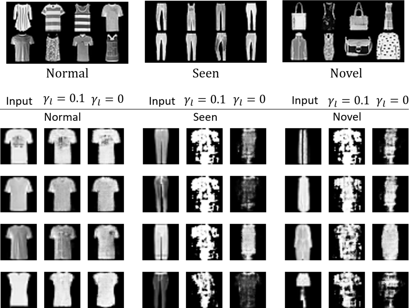
Considering that the image patterns in F-MNIST are easy to identify, we train our proposed model under different collected-anomaly ratio on the F-MNIST dataset and then select the reconstructed images from the testing datasets to show in Fig. 5. The case with corresponds the scenario without using any anomalies during the training. It can be observed that for normal samples, whether utilizing the collected anomalies or not, the images can be well reconstructed. But without the leverage of collected anomalies, AA-BiGAN() seems to reconstruct the anomaly samples as well. The reconstruction of the anomalous samples output by the AA-BiGAN() has a very similar shape contour to the original data. As long as a proportion() of collected anomalies are leveraged, the reconstructed images of anomalies becomes blurry and noise, brings a significant difference between original images and reconstructed images. The comparison of reconstructed images intuitively explain how our model yields more discriminative reconstruction error criteria for better detection.
Generation Ability Assessment
Extensive experiments are conducted to verify our proposed model’s generation quality. Fig. 6 shows our model can generate high quality images which patterns are easy to distinguish. To further evaluate the our model’s generation ability, we conduct experiments referring to Lucic et al. 2018 settings. In each experiment, we regard one category as anomalies and train on the other nine categories. We train epochs for F-MNIST and MNIST and epochs for CIFAR-10, with the best observed FID to be reported. Although the main propose of our model is to enhance the distinguishability between normal and anomaly samples rather than obtaining high quality generated images, it can still be observed that our model’s FID score is overall in the same level as existing generative models, showing the generation ability of our proposed model.
| MNIST | F-MNIST | CIFAR-10 | |
| GAN | 9.8 0.9 | 29.6 1.6 | 72.7 3.6 |
| WGAN | 6.7 0.4 | 21.5 1.6 | 55.2 2.3 |
| LSGAN | 7.8 0.6 | 30.7 2.2 | 87.1 47.5 |
| VAE | 40.1 0.7 | 100.9 3.0 | 155.7 11.6 |
| AA-BiGAN | 8.9 1.0 | 27.2 1.8 | 111.3 10.1 |


Sensitivity Analysis
We analyze the major hyperparameter of our proposed method. According to our developed theories, the parameter could be set arbitrarily, in practical it better not make equal to , and . We evaluate the performance of our model under four different values of , which is shown in Table 5. It can be seen that the performance is not sensitive to . The results show that the best performance can be obtained when keeping the value of far away from the target value of other parameters. We thus set always to 3/4.
| 0.25 | 0.4 | 0.6 | 0.75 | |
| , | 94.5 4.3 | 94.4 4.3 | 94.5 4.2 | 94.6 4.2 |
| , | 91.6 5.0 | 91.3 5.3 | 91.3 5.2 | 91.8 4.9 |
| Data | OCSVM | Deep SVDD | ALAD | CAE | SSAD Raw | SSAD Hybrid | SS-DGM | Deep SAD | Supervised Classifier | NDA | AA-BiGAN (Ours) | |
| .00 | 96.3 2.5 | 92.8 4.9 | 96.2 3.3 | 92.9 5.7 | 97.9 1.8 | 97.4 2.0 | 92.2 5.6 | 96.7 2.4 | 94.5 4.6 | 96.8 3.2 | 97.8 2.0 | |
| .01 | 95.6 2.5 | 92.1 5.1 | 93.3 4.2 | 91.3 6.1 | 96.6 2.4 | 95.2 2.3 | 92.0 6.0 | 96.4 2.7 | 91.5 5.9 | 96.4 2.7 | 96.9 2.3 | |
| MNIST | .05 | 93.8 3.9 | 89.4 5.8 | 92.6 5.2 | 87.2 7.1 | 93.4 3.4 | 89.5 3.9 | 91.0 6.9 | 93.5 4.1 | 86.7 7.4 | 93.2 4.9 | 95.1 3.0 |
| .10 | 91.4 5.1 | 86.5 6.8 | 91.0 5.6 | 83.7 8.4 | 90.7 4.4 | 86.0 4.6 | 89.7 7.5 | 91.2 4.9 | 83.6 8.2 | 90.4 5.9 | 93.2 4.3 | |
| .20 | 85.9 7.6 | 81.5 8.4 | 88.0 6.2 | 78.6 10.3 | 87.4 5.6 | 82.1 5.4 | 87.4 8.6 | 86.6 6.6 | 79.7 9.4 | 87.3 6.8 | 90.8 5.1 | |
| .00 | 91.2 4.7 | 89.2 6.2 | 91.1 5.3 | 90.2 5.8 | 94.0 4.4 | 90.5 5.9 | 71.4 12.7 | 90.5 6.5 | 76.8 13.2 | 91.0 7.0 | 94.6 4.2 | |
| .01 | 91.5 4.6 | 86.3 6.3 | 91.3 4.2 | 87.1 7.3 | 92.2 4.9 | 87.8 6.1 | 71.2 14.3 | 87.2 7.1 | 67.3 8.1 | 89.8 8.6 | 94.1 4.3 | |
| F-MNIST | .05 | 90.7 4.9 | 80.6 7.1 | 90.5 4.5 | 81.6 9.6 | 88.3 6.2 | 82.7 7.8 | 71.9 14.3 | 81.5 8.5 | 59.8 4.6 | 87.5 10.5 | 93.1 4.6 |
| .10 | 89.3 6.2 | 76.2 7.3 | 89.6 4.5 | 77.4 11.1 | 85.6 7.0 | 79.8 9.0 | 72.5 15.5 | 78.2 9.1 | 56.7 4.1 | 85.1 12.9 | 91.8 4.9 | |
| .20 | 88.1 6.9 | 69.3 6.3 | 88.3 4.6 | 72.5 12.6 | 81.9 8.1 | 74.3 10.6 | 70.8 16.0 | 74.8 9.4 | 53.9 2.9 | 80.7 15.1 | 90.2 5.2 | |
| .00 | 63.8 9.0 | 60.9 9.4 | 65.0 9.4 | 56.2 13.2 | 73.8 7.6 | 73.3 8.4 | 50.8 4.7 | 77.9 7.2 | 63.5 8.0 | 78.9 7.7 | 81.2 6.4 | |
| .01 | 63.8 9.3 | 60.5 9.4 | 65.4 9.8 | 56.2 13.1 | 73.0 8.0 | 72.8 8.1 | 51.1 4.7 | 76.5 7.2 | 62.9 7.3 | 78.2 7.1 | 81.9 6.6 | |
| CIFAR-10 | .05 | 62.6 9.2 | 59.6 9.8 | 65.1 9.3 | 55.7 13.3 | 71.5 8.2 | 71.0 8.4 | 50.1 2.9 | 74.0 6.9 | 62.2 8.2 | 76.0 7.0 | 81.1 6.7 |
| .10 | 62.9 8.2 | 58.6 10.0 | 64.4 9.3 | 55.4 13.3 | 54.6 13.3 | 69.3 8.5 | 50.5 3.6 | 71.8 7.0 | 60.6 8.3 | 74.5 7.7 | 78.2 7.1 | |
| .20 | 61.9 8.1 | 57.0 10.6 | 64.2 9.4 | 54.6 14.3 | 67.8 8.6 | 67.9 8.1 | 50.1 1.7 | 68.5 7.1 | 58.5 6.7 | 72.1 8.5 | 77.0 8.1 |
| Data | OCSVM | Deep SVDD | ALAD | CAE | SSAD Raw | SSAD Hybrid | SS-DGM | Deep SAD | Supervised Classifier | NDA | AA-BiGAN (Ours) | |
| 0 | 91.4 5.1 | 86.5 6.8 | 91.0 5.6 | 83.7 8.4 | 88.0 6.0 | 91.4 5.1 | 86.5 6.8 | 88.5 6.4 | 91.0 5.6 | |||
| 1 | 90.7 4.4 | 86.0 4.6 | 89.7 7.5 | 91.2 4.9 | 83.6 8.2 | 90.4 3.9 | 94.5 3.7 | |||||
| MNIST | 2 | 92.5 3.6 | 87.7 3.8 | 92.8 5.3 | 92.0 3.6 | 90.3 4.6 | 94.7 3.2 | 95.9 2.7 | ||||
| 3 | 93.9 3.3 | 89.8 3.3 | 94.9 4.2 | 94.7 2.8 | 93.9 8.6 | 96.0 3.0 | 96.3 2.7 | |||||
| 5 | 95.5 2.5 | 91.9 3.0 | 96.7 2.3 | 97.3 1.8 | 96.9 1.7 | 97.9 1.6 | 97.7 1.5 | |||||
| 0 | 89.3 6.2 | 76.2 7.3 | 89.6 4.5 | 77.4 11.1 | 89.5 6.1 | 89.3 6.2 | 76.2 7.3 | 73.3 18.2 | 91.0 4.5 | |||
| 1 | 85.6 7.0 | 79.8 9.0 | 72.5 15.5 | 78.2 9.1 | 56.7 4.1 | 85.1 12.9 | 92.3 5.1 | |||||
| F-MNIST | 2 | 87.8 6.1 | 80.1 10.5 | 74.3 15.4 | 80.5 8.2 | 62.3 2.9 | 90.2 7.9 | 93.6 4.6 | ||||
| 3 | 89.4 5.5 | 83.8 9.4 | 77.5 14.7 | 83.9 7.4 | 67.3 3.0 | 92.2 6.7 | 94.2 4.4 | |||||
| 5 | 91.2 4.8 | 86.8 7.7 | 79.9 13.8 | 87.3 6.4 | 75.3 2.7 | 95.3 4.5 | 95.3 4.4 | |||||
| 0 | 62.9 8.2 | 58.6 10.0 | 64.4 9.3 | 55.4 13.3 | 60.8 10.7 | 62.9 8.2 | 58.6 10.0 | 64.2 6.4 | 65.4 9.1 | |||
| 1 | 69.8 8.4 | 69.3 8.5 | 50.5 3.6 | 71.8 7.0 | 60.6 8.3 | 74.5 7.7 | 78.2 7.1 | |||||
| CIFAR-10 | 2 | 73.0 7.1 | 72.3 7.5 | 50.3 2.4 | 75.2 6.4 | 61.0 6.6 | 75.9 8.1 | 84.3 6.1 | ||||
| 3 | 73.8 6.6 | 73.3 7.0 | 50.0 0.7 | 77.5 5.9 | 62.7 6.8 | 76.8 7.6 | 85.6 5.8 | |||||
| 5 | 75.1 5.5 | 74.2 6.5 | 50.0 1.0 | 80.4 4.6 | 60.9 4.6 | 78.8 6.2 | 87.8 5.2 |
| Data | OCSVM Hybrid | CAE | NDA | Deep SVDD | AAD | SSAD Hybrid | SS-DGM | Supervised Classifier | Deep SAD | AA-BiGAN (Ours) |
| Arrhythmia | 76.7 6.2 | 74.0 7.5 | 74.1 8.9 | 74.6 9.0 | 75.8 3.2 | 78.3 5.1 | 50.3 9.8 | 39.2 9.5 | 75.9 8.7 | 80.7 3.2 |
| Cardio | 82.8 9.3 | 94.3 2.0 | 86.0 5.8 | 84.8 3.6 | 90.7 2.1 | 86.3 5.8 | 66.2 14.3 | 83.2 9.6 | 95.0 1.6 | 98.0 1.2 |
| Satellite | 68.6 4.8 | 80.0 1.7 | 78.0 3.3 | 79.8 4.1 | 77.2 4.1 | 86.9 2.8 | 57.4 6.4 | 87.2 2.1 | 91.5 1.1 | 87.4 2.3 |
| Satimage-2 | 96.7 2.1 | 99.0 0.0 | 94.8 2.3 | 98.3 1.4 | 99.9 0.1 | 96.8 2.1 | 99.2 0.6 | 99.1 0.1 | 99.9 0.1 | 99.9 0.1 |
| Shuttle | 94.1 9.5 | 98.2 1.2 | 98.2 0.5 | 86.3 7.5 | 99.0 0.2 | 97.7 1.0 | 97.9 0.3 | 95.1 8.0 | 98.4 0.9 | 99.1 0.1 |
| Thyroid | 91.2 4.0 | 75.2 10.2 | 91.9 4.5 | 72.0 9.7 | 96.5 0.8 | 95.3 3.1 | 72.7 12.0 | 97.8 2.6 | 98.6 0.9 | 98.9 0.1 |
Empirical Study of Computational Efficiency
We investigate the training complexity by comparing the training duration of our method and ALAD Zenati et al. 2018b. Theoretically, our model employs the same network architecture as ALAD model, the only difference is that we have added one more term to the updating function. Thus the complexity of our method is similar to the baseline ALAD model. On the F-MNIST and CIFAR-10 datasets, the one-epoch training time of our model is 8.833 seconds and 10.108 seconds, while that of the ALAD model is 7.924 seconds and 8.729 seconds. It can be seen that our model, though with much stronger performance, can be trained almost as efficiently as ALAD.
Complete Tables of Experimental Results
In addition to the semi-supervised models Görnitz et al. 2013; Kingma et al. 2014; Ruff et al. 2019; Sinha et al. 2020; Das et al. 2020 mentioned in the main paper text, we also consider some unsupervised models Schölkopf et al. 2001; Ruff et al. 2018; Zenati et al. 2018b for comparison. Table 6 lists the complete experimental results as a function of pollution ratio on the three image datasets, in which the ratio of available anomalies is fixed as 0.05. Specifically, an averaged improvement of , , on MNIST, F-MNIST, CIFAR-10 are observed. As the pollution ratio increases from 0.0 to 0.2, the superiority of our model is even more evident. Another noteworthy point is that ALAD model Zenati et al. 2018b also appear to be more robust than distance-based models, which further confirms that the GAN-based probabilistic methods are often more tolerant of data pollution than the distance-based methods.
Table 7 lists the specific experimental results as a function of the number of categories of collected anomalies increases, in which and are fixed as 0.05 and 0.1. Our proposed model improves the average performance by , , on MNIST, F-MNIST, CIFAR-10. On the specific CIFAR-10 dataset, thanks to the strong ability of GANs in modeling the complex images, our model achieves a remarkable improvement in all level.
Table 8 lists the complete experimental results on tabular dataset. With the strong modeling capacity of deep neural networks, our proposed batch-processing model achieve an average improvement of performance compared to AAD. In comparison with the distance-based methods, the competitive results can be observed, which demonstrating the effectiveness of the proposed probabilistic method on classic anomaly detection datasets.