SSR-GNNs: Stroke-based Sketch Representation with Graph Neural Networks
Abstract
This paper follows cognitive studies to investigate a graph representation for sketches, where the information of strokes, i.e., parts of a sketch, are encoded on vertices and information of inter-stroke on edges. The resultant graph representation facilitates the training of a Graph Neural Networks for classification tasks, and achieves accuracy and robustness comparable to the state-of-the-art against translation and rotation attacks, as well as stronger attacks on graph vertices and topologies, i.e., modifications and addition of strokes, all without resorting to adversarial training. Prior studies on sketches, e.g., graph transformers, encode control points of stroke on vertices, which are not invariant to spatial transformations. In contrary, we encode vertices and edges using pairwise distances among control points to achieve invariance. Compared with existing generative sketch model for one-shot classification lake2015human, our method does not rely on run-time statistical inference. Lastly, the proposed representation enables generation of novel sketches that are structurally similar to while separable from the existing dataset.
1 Introduction
Unlike the human vision system, it is well acknowledged that end-to-end deep learning methods lack intermediate representations that enable innate invariance to spatial translation and rotation hinton2021represent; hinton1979some; bi2017; popsci2017; levesque2011winograd; clark2015elementary; newyorker2013; nytimes2017gm.
While such transformation invarianace can potentially be achieved through expensive robust (adversarial) training, it is believed that invariance (1) should be an innate property rather than an external model constraint, and (2) should not trade off recognition accuracy significantly. This motivates us to revisit the canonical computer vision perspective (such as object representation by components biederman1987recognition, and local visual representation design lowe2004distinctive) towards an explicit representation design for possessing innate properties.
A commonly sought-after solution is to identify a part-whole structure hinton2021represent, following the insights of how the human vision system hinton1979some; biederman1987recognition parses scenes into atomic parts for recognition and generation, while both parts and the topologies of parts are invariant to spatial transformations. The part-whole structure is also supported by the Gestalt principles desolneux2007gestalt and cognitive science lake2017building; lake2012concept; lake2015human.
Building on top of existing work and within the context of computer vision for sketch recognition, we present a part-whole representation where strokes, as parts, are connected as a graph to form a sketch. The focus on sketches draws inspiration from studies in biology and cognitive science kubilius2016deep; landau1988importance; ha2017neural; ritter2017cognitive. For example, landau1988importance; ritter2017cognitive show that human vision relies more on shapes than on textures or colors. Studies also show that successful CNNs learn shape representations from natural images geirhos2018imagenettrained; kriegeskorte2015deep; kubilius2016deep; hosseini2018assessing.
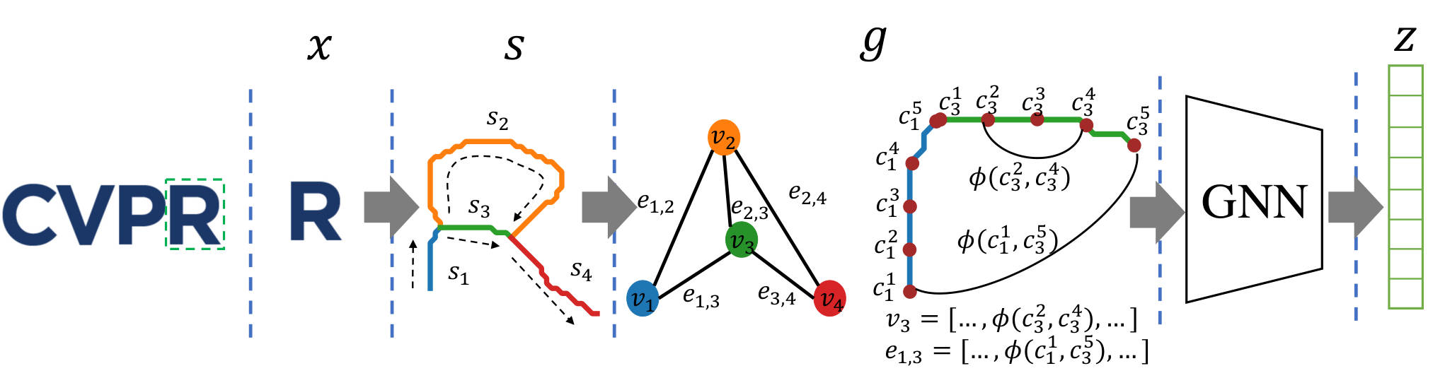
Fig. 1 shows an example of the proposed representation: From an input image of “R”, we adopt unsupervised image processing lake2015human to first identify fork points that separate strokes, and estimate control points of these strokes to form an undirected graph representation where each vertex contains stroke information, and edges specify interactions between strokes. Specifically, to innately equip our representation with spatial invariance, each vertex encodes pairwise spatial distances between each pair of control points for the corresponding stroke (see in Fig. 1), yielding an matrix. If two strokes (each with control points) are connected, we then form an edge in the resulting graph. The edge encodes the pair-wise distance between each control point from one stroke to each of the other stroke (see in Fig. 1). The distances between control points are invariant to spatial transformations, therefore our graph design is innately spatially-invariant.
To validate this representation, we take sketch-based classification/robust feature learning, and novel pattern generation as the testing tasks. To leverage the graph representation for classification, we train a Graph Neural Network (GNN) scarselli2008graph, which allows variable input graph topologies and preserves spatial invariance.
We claim the following contributions:
- •
Through extensive experiments on MNIST and two subsets of the Quickdraw dataset ha2017neural, we show that the proposed models are innately robust to rotations and translations, while maintaining acceptable classification accuracy.
- •
In addition, we show that the proposed models are robust to parametric and topological attacks without robust training, which suggests that stroke-based graphs are robust features for perception.
- •
Lastly, we show that the proposed models can be used to generate novel sketchs distinguishable from the training set. E.g., by learning to classify decimal digits, the model can then be used to generate hypothetical “A”s to “F”s for a hexadecimal system. This shows that models have strongly structured expression capability.
2 Related work
Part-whole representations: Studies in cognitive science suggest the human vision system parse visual inputs into part-whole, which are invariant to spatial transformations and change of viewpoints hinton2021represent; sabour2018matrix; singh2001part. For example, structural description models biederman1987recognition; hummel1992dynamic; van2015part; kodratoff1984learning combine the description of the part components. Along the same vein, sketches have been considered as a composition of strokes which are parts and sub-parts representation lake2015human. Such part-whole representations have been shown to play a critical role in enabling learning with small data. lake2015human shows that one-shot classification/generation can be achieved on labeled graphs through iterative inference based on statistics of sampled graphs.
Graph neural network: In graph neural networks (GNNs) duvenaud2015convolutional; bruna2013spectral, vertex and edge information evolve through neighborhood aggregation. By sharing pairwise aggregation models, such as in message passing neural networks (MPNNs) gilmer2017neural; li2015gated, GNNs are often shown to be generalizable to input graphs with arbitrary sizes. They are widely used in the area of sketches yang2020sketchgcn, handwriting riba2015handwritten and math formula recognition mahdavi2020visual. In this work, we adopt an MPNNs architecture to handle sketches with variable number of strokes and topologies. Graph-based representation cho2013learning; wu2014learning or graph neural network gilmer2017neural; li2015gated are also invariant to permutation. In this work, the high level representations are inputs transformation invariant because both stroke representation and graph neural network are invariant to transformation.
Sketch-based learning: Sketch is an abstract visual input without the information of texture and color xu2020deep. Cognitive science research shows that human beings are able to grasp the major semantic meaning from an image directly from its sketch form kriegeskorte2015deep. Current studies typically primarily investigate sketch classification using existing deep neural networks. CNNs based methods yu2017sketch; song2017deep are applied on raster sketch image. RNNs based methods xu2018sketchmate; jia2017sequential; he2017sketch; ha2017neural; xu2020learning, as well as textual convolution network (TCN) xu2020deep, transformer (Sketchformer) ribeiro2020sketchformer, model sketch as sequence of control points or strokes. Graph based methods yang2021sketchgnn; xu2021multigraph; yang2021sketchaa; yang2020sketchgcn explore the topological information for sketch. Graph transformer xu2021multigraph encodes the control point as vertex and 1-hop, 2-hop, global hop connection as edge. SketchAA yang2021sketchaa learns the abstraction and hierarchy of the grid blocks of sketch image by encoding them as graph. SketchGNN yang2021sketchgnn learns the semantic segmentation of sketch. The vertex of SketchGNN is the single point on sketch and the edge is the single stroke that connecting two adjacent points. Furthermore, current studies of sketch are extended to multimodality, such as sketch with video xu2020fine; collomosse2009storyboard, sketch with word, text, cartoon and natural image xie2019deep. In this work, unlike the previous works which only focus on improving the classification accuracy only, we take sketch based classification as a testing task to validate that the newly proposed representation design is spatially robust. Especially in adversarial cases, our sketch classification maintains a high level of performance.
3 Methods
Our method contains the following elements: (1) A pre-process step where an input image is converted to a set of strokes . (2) The strokes and their connections are then encoded as a graph . Node and edge features are designed to achieve rotation and translation invariance. (3) A GNN is learned based on a labeled dataset . Fig. 1 summarizes the learning pipeline. Details are explained as follows.
3.1 Acquiring Strokes from an Image
We decompose an input image into a set of strokes, denoted by , where varies by image. We follow the preprocess procedures of lake2015human, which include thinning the image lam1992thinning, detecting fork points liu1999identification, and finally merging the noisy and redundant fork points by the maximum circle criterion liao1990stroke. The ordering of the strokes, i.e., the definition of the start and end points of strokes, is then derived from a walk throughout the fork points which follows the rules moving from left to right and from top to bottom. Fig. 1 demonstrates the procedure for “R”.
Building upon lake2015human, each stroke is first approximated as a uniform cubic b-spline parameterized by the control points, the offset, and the scaling factor. We then sample control points on stroke by re-fitting the uniform cubic b-spline. The number of control points are set to be the same for all strokes and tuned for each experiment. Unlike lake2015human which takes a set of uniform cubic b-spline control points, we set aside the offset for enforcing boundary constraints, and the scale factor for accurately computing the pairwise distances. We represent a stroke using its control points: .
3.2 Stroke-based Graph Representation
We further convert the set of strokes into a graph , where each vertex corresponds to a stroke , and an edge exists when the start (end) point of is the end (start) point of . To achieve rotation and translation invariance, we assign each vertex the set of pairwise Euclidean distances between all sample points from . In particular, where is the th control point of the th stroke and is the Euclidean distance. Similarly, we assign each edge the set of pairwise Euclidean distances from all control points from to those from : . We note that the ordering of elements in and is defined based on the start and end points of and , i.e., switching the start and end points of will change and .
3.3 GNN architecture
We adopt MPNNs to handle the variable graph sizes encountered in MNIST and QuickDraw datasets. The MPNN contains three components: (M) message passing, (U) update, and (R) readout battaglia2018relational, which are defined as:
The message passing and update phase execute times. The message at phase , , is encoded by vertex , adjacent vertices s and edges at step . The new vertex is updated by current vertex and message . After steps, the feature is computed from a readout function. , , are learnable components. is input to a linear classifier with softmax outputs. To simplify the notation, we define the MPNN as and linear classifier as .
3.4 Learning Objectives
Here we introduce the formulations of the learning problems for the two experiments to be discussed in Sec. 4.
Classification
We use a standard cross-entropy loss for learning a classifier . Given a dataset , the loss is:
| (1) |
where is the cross-entropy.


 (a) MNIST
(b) Quickdraw(Shape)
(c) Quickdraw(Body)
(a) MNIST
(b) Quickdraw(Shape)
(c) Quickdraw(Body)
Sketch modification and generation
In experiments, we will demonstrate the robustness of the classifier against targeted attacks via vertex-wise and topology-wise perturbations. For topology-wise attacks, we specifically consider adding a stroke to an existing sketch. In both cases, we let the target label be a one-hot vector , the set of control points of the stroke of interest be and the resultant graph be . The attacks solve:
| (2) |
where , as explained below, constrains the control points to be structurally similar to the training data. In addition, we also incorporate boundary constraints on to limit the generated sketches within the boundaries of the image.
Penalty on sketch structure: We consider two types of penalties on a generated graph to regulate its structure. First, the generated sketches should have pairwise distances between control points similar to those from the training data. Second, the angles between neighbouring pairs of control points, denoted by , should also be similar to those from the data. We incorporate these requirements through the following penalty:
| (3) | ||||
where and are the empirical distributions of the pairwise distances among control points within a stroke and between strokes from the dataset, respectively, and, is that of the angles between neighbouring pairs of control points. and are tuned to allow the attack loss to dominate.
We will also demonstrate the utility of the proposed model at generating new sketches that are structurally similar to the training data, yet semantically different. To do so, we first train a one-class classifier so that all training data belongs to the same group, i.e., for all . Given a sketch parameterized by the set of control points to be tuned, we solve the following problem
| (4) |
The hinge loss used here aims to push the generated sketch out of the training set.
| Method | Evaluation | MNIST | Quickdraw (Shape) | Quickdraw (Body) |
|---|---|---|---|---|
| CNNs engstrom2019exploring; xu2021multigraph | Accuracy | 99.31% | 87.14% | 80.10% |
| Spatial Robustness | 26.02% | 21.90% | 31.10% | |
| Parameter Size | 600,810 | 25,315,474 | 25,315,474 | |
| RNNs xu2021multigraph | Accuracy | - | 75.43% | 68.30% |
| Spatial Robustness | - | 0.00% | 0.00% | |
| Parameter Size | - | 5,724,249 | 5,724,249 | |
| Graph Transformer xu2021multigraph | Accuracy | - | 80.71% | 75.4% |
| Spatial Robustness | - | 0.10% | 6.57% | |
| Parameter Size | - | 39,984,729 | 39,984,729 | |
| Ours | Accuracy | 93.01% | 73.00% | 64.20% |
| Spatial Robustness | 93.01% | 73.00% | 64.20% | |
| Parameter Size | 546,634 | 8,707,868 | 8,707,868 |
4 Experiments
We conduct two sets of experiments. First, we empirically show that the proposed model is robust to rotation and translation on classification tasks for MNIST and a subset for QuickDraw, while maintaining accuracy comparable to the SOTA, all without adversarial training. We also evaluate model robustness against vertex-wise and topology-wise attacks specific to graph inputs. Second, we show that our model is capable of generating novel sketches that are semantically different from the training set. Specifically, we demonstrate the generation of hypothetical digits that are separable from MNIST digits in the feature space.
4.1 Classification and Robustness
Dataset and pre-processing
We use two standard datasets: MNIST and Google Quickdraw ha2017neural. MNIST is a hand-written digit dataset containing numerical digits from -. Google Quickdraw is a human hand-drawn sketch dataset with different categories, ranging from The Great Wall, airplane, to hands, squares, and dogs. For both datasets, we consider each sketch as an image, shifted to the top-left corner and normalized to pixels. It should be noted that the Quickdraw dataset also stores key points of simplified strokes in temporal order xu2021multigraph; xu2018sketchmate, computed by the Ramer-Douglas-Peucker algorithm ramer1972iterative. This format has been used by existing graph-based classifiers xu2021multigraph and recurrent neural networks xu2018sketchmate. However, this format represents sketches as graphs with a large variance of sizes, e.g., some sketches have multiple strokes with negligible lengths. To this end, we preprocess the data by extracting strokes from the pixelated sketches using the method introduced in Sec. 3.1, while preserving the information about the start and end points of the extracted strokes. During this process, we delete strokes with negligible lengths less than 5 pixels.
We also note that due to the abstract nature of sketches in some categories of Quickdraw, we only adopt two subsets of the dataset for our experiments. The first subset contains all shape categories including circle, hexagon, line, octagon, square, triangle, zigzag (see Fig. 2(b)), and the second contains all body categories including arm, ear, elbow, face, finger, foot, hand, nose, toe, tooth (see Fig. 2(c)). For both subsets, we select , , samples per category for training, validation and testing, respectively. To avoid strokes being moved out of the image through transformations during robustness evaluation, we zero-pad the image with 40 pixels on each side. Since the strokes in the sketch image are mostly short ones, we set the number of control points on each stroke to for all experiments. We also notice the existence of complicated fork points, i.e., a small cluster of connected strokes in place of a single fork point, due to the use of the maximum circle criterion. To this end, we dilate the sketch with 4 pixels which addresses this issue.
Network architecture and training details
We adopt MPNN from Sec. 3.3 following the same architecture as the gated graph neural networks (GG-NNs) li2015gated. The message passing function is
| (5) |
The update function is a Gated recurrent unit cho2014properties, where . The readout function is
| (6) |
For MNIST, each is a linear four-layer fully-connected network, with the intermediate feature sizes as , , and . The message passing iterations is set to 1 and the final feature vector size is set to 10. We use the batch size , with an initial learning rate . To handle the complex images in Quickdraw, we increase the depth of our architecture to linear layers and the dimensions of the intermediate features are , , , , , , . The message passing iterations is set to and the dimension of the final feature vector is . We set the the batch size as eight with an initial learning rate using the SGD optimizer. The objective function follows Eq. 1.
Baselines
Convolutional Neural Networks (CNNs): On MNIST, we train a CNN with two convolutional layers and two linear layers maintaining comparable learnable parameters to our model for fair comparisons. On Quickdraw, we choose the Inception network szegedy2015going as the baseline.
Recurrent neural networks (RNNs) ha2017neural encodes a sketch as a sequence of key points and flag bits, indicating the start or end of the strokes. SketchMate xu2018sketchmate fuses the CNN encoding with the RNN encoding. In our experiment, We use a bi-directional GRU as a baseline.
Graph based networks xu2021multigraph, including graph convolution network (GCN), graph attention network (GAT) and graph transformer, encode a sketch as graph. We choose graph transformer as our baseline since it shows better performance than GCN and GAT. This method is different from ours: Each vertex is a key point of a stroke, represented by the corresponding coordinates. Therefore, this representation is not invariant to spatial transformations. In addition, Graph Transformer based methods need information about the start or end points of the strokes as inputs. In our method, we extract this information from fork point detection.
Step 0
Step 0
Step 100
Step 1000
Last step
Last step
Image
1(0.9928)
7(0.9862)
7(0.9907)
7(0.9963)
Image
(a)

 Step 0
Step 100
Step 1000
Last step
Last step
Image
6(0.9789)
9(0.4573)
0(0.9640)
0(0.9952)
Image
(d)
Step 0
Step 0
Step 100
Step 1000
Last step
Last step
Image
6(0.9789)
9(0.4573)
0(0.9640)
0(0.9952)
Image
(d)


1(0.9964)
1(0.7139)
7(0.6389)
7(0.9788)
(b)

 6(0.9773)
6(0.8451)
0(0.8163)
0(0.9946)
(e)
6(0.9773)
6(0.8451)
0(0.8163)
0(0.9946)
(e)


7(0.9999)
7(0.5978)
2(0.8600)
2(0.9655)
(c)

 7(0.9995)
7(0.6192)
1(0.9312)
1(0.9911)
(f)
7(0.9995)
7(0.6192)
1(0.9312)
1(0.9911)
(f)


Evaluation
To evaluate the spatial robustness of the model, we apply rotation and translation attacks on the input images following engstrom2019exploring:
| (7) |
for pixel coordinates . For MNIST, we rotate within and translate within pixels. For Quickdraw, since the image size increases, we increase the maximum translation to pixels. To generate the transformed images, we discretize the parameters to grids of rotations and translations (as shown in Fig. 2). We sample values per translation direction and values for rotations. Together, the procedure yields transformed samples per image. If one of the transformed images has incorrect predicted label through , the model is not considered robust against the transformation with respect to that particular image engstrom2019exploring.
 6:0.908
9:0.085
6:0.908
9:0.085
 6:0.918
9:0.002
6:0.918
9:0.002
 6:0.988
9:0.000
6:0.988
9:0.000
 6:0.000
9:1.000
6:0.000
9:1.000
 6:0.000
9:0.997
6:0.000
9:0.997
 6:0.001
9:0.998
6:0.001
9:0.998
 6:0.000
9:1.000
6:0.000
9:1.000
 6:0.000
9:0.999
6:0.000
9:0.999
 6:0.997
9:0.000
6:0.997
9:0.000
 6:0.970
9:0.024
6:0.970
9:0.024
 6:0.973
9:0.019
6:0.973
9:0.019
 6:1.000
9:0.000
6:1.000
9:0.000
Classification and spatial robustness results
Table 1 summarizes the experimental results. (1) For accuracy, CNNs achieve the best results. Our method achieves comparable accuracy on MNIST and slightly inferior ones on Quickdraw subsets. The accuracy gaps between ours and other baselines, i.e., RNNs and graph transformers, are smaller on Quickdraw subsets. Note that these models do not work directly on MNIST as they require temporal information of the strokes. (2) Our stroke representation is invariant to rotations and translations, and therefore its robustness stays the same as its accuracy. We highlight that our model outperforms baselines on spatial robustness by a large margin. The robustness of CNNs drops to , , on the three experiments. And the robustness of RNNs and graph transformers are less than on Quickdraw subsets. (3) Our models are also efficient parameter-wise, using only % and % of parameters of Inception-V3 and Graph Transformers, respectively.
Robustness against graph attacks
Previous studies have explored the connection between model robustness and the learning of robust features, i.e., features that are invariant to attacks NEURIPS2019_e2c420d9; tsipras2018robustness. The above experiments show that our model is robust to attacks in the form of global transformations. In addition, the procedure of stroke extraction is robust to conventional pixel-wise attacks due to its thinning and merging steps. Here, we further investigate the robustness of our model under graph-specific attacks. If successful, our study provides evidence that the proposed graph representation contains robust features that enable model robustness without adversarial training.
Altering the graph topology: In this experiment, we consider adding/deleting vertices to alter the graph topology. We conduct the experiment by adding one stroke, denoted by , on digit “1”s with a single stroke . We optimize using Eq. (2) by targeting the resultant graph to be classified as digit “7”. Since our representation is spatially invariant, the start point of is fixed and connected to either side of and all other trainable control points of are initialized with the same values as the start point. The procedure to get follows the setting described in Sec. 3.4: We apply penalties on angles and pairwise distances, where in Eq. 3 denotes the set of two-stroke “7”s.
We visualize in Fig. 3(a) the evolution of the added stroke during the optimization of Eq. (2). Part of the new stroke evolves towards being flat at step 100, while the converged stroke becomes flat. Similar experiments are shown in Fig. 3(b,c) on modifying “1” to “7”, and “7” to “2”. Considering that our model is rotation (and mirror) invariant, the results suggest that the graph representation is robust in that when the attacks are successful, the contents of the images have to be changed semantically towards the target labels.
It should also be noted that while a rotated “7”, as in Fig. 3(b), should not be considered as a “7” from human perspective, this only happens because the added stroke is considered to move from right to left (as the first stroke of the connected two). The stroke extraction procedure described in Sec. 3.1 considers strokes to move from left to right and top to down, and therefore will avoid classifying the outcome of Fig. 3(b) as “7” (since the added stroke will be considered as the second stroke of the sequence and moves from left to right). This also explains why our model can correctly classify “6” and “9” even with its invariance property in Fig. 4: We set the strokes of the two to have different start and end control points.
Lastly, the results in Fig. 3(a) reveals that our model is in fact invariant to mirroring (here the added stroke will be considered as moving from right to left through the stroke extraction procedure, and thus its graph representation is equivalent to its mirrored version). While this invariance is undesirable, it is in fact commonly observed as a property of human vision system during its early phase (e.g., among children). For example, when start learning to write, children may consider ‘‘b’’ and ‘‘d’’, ‘‘p’’ and ‘‘q’’, ‘‘J’’ and ‘‘L’’ the same, as well as writing mirrored digits 11 1 This is observed from one of the authors’ 5yr old, and confirmed by her teacher.. Removing the mirror invariance property through representation design or learning, will be deferred to a future study.


 A
B
C
A
B
C


 D
E
F
D
E
F
 (a) Generated 6 new digits
(b) The generated image’s high level distribution
(a) Generated 6 new digits
(b) The generated image’s high level distribution
Modifying control points In addition to robustness against changes in graph topologies, we show that our model is also robust against changes to control points of strokes (and therefore the graph representation). To this end, we tune the coordinates of the control points of a “6” towards label “0” using Eq. (2). in the attack loss is set to the set of all “0”s with a single stroke. Fig. 3(d) shows evolution of the sketch during the attack. At step 0, the image is recognized as “6” with a high confidence. While altering the control points at step 100, it is recognized as “9” with a confidence score (while “0” and “6” receive scores of only and . For the final step, the model recognizes the altered image as “0”, with a high confidence. We show experimental results on other input samples in Fig. 3(e,f). Again, results suggest that the graph representation is robust as successful attacks need to alter the semantic meaning of the sketches.
4.2 New digits generation
Here we demonstrate that the graph representation enables generation of novel sketches that are separable in the feature space from the training data, while maintaining structural similarity. The underlying rationale is that if our stroke-based graph representation is with strongly structured expression capability, the underlying feature space after supervised training on existing categories could guide a generation process to come up with new categorical patterns.
The formulation of the generation problem follows Eq. 4. To initialize a solution, we draw the control points of a new digit from a normal distribution , where the mean is randomly sampled in a uniform distribution ranging from 4 to 24, and is initially set to . We consider cases where the graph topology is fixed. Alg. 1 explains the procedure for solving Eq. 4, with two alternating steps. In the first step, we focus on separating the new set from the existing dataset . Fixing the feature extractor MPNN , the binary classification objective function is given as:
| (8) | ||||
In the second step, we update the distribution of through and following Eq. 4. The dataset here in the loss function is the entire MNIST training set.
In our experiment, we generate a sequence of novel digits with a single stroke that are separable from the MNIST digits in the feature space, as illustrated in Fig. 5(a). It is worth noting that the newly generated digits share a similar visual style to MNIST hand-written digits (although a quantitative analysis will require a Turing test lake2015human), and at the same time visually distinguishable from them. Fig. 5(b) further confirms our claim, as we can see that on the space formed by the final MPNN network, all novel digits are separable from each other, and are distinguishable from the original set. The new digits generation experiment validates that our model has a strong structured expression capability.
blueberry
broom


 paintbrush
toaster
paintbrush
toaster


5 Limitations
End-to-end stroke extraction The major limitation in our method is in the preprocessing step. As shown in Fig. 6, many data points from the Quickdraw dataset contain strokes that form detailed parts of a whole or textures of parts, some of which can be quite abstract (see “blueberry” for example). Our stroke extraction procedure currently cannot correctly infer the stroke sequences of such sketches or produce abstraction of clustered strokes, e.g., those that represent a part with texture. To achieve this, we hypothesize that it is necessary to express the stroke extraction procedure as a differentiable program, so that it can be learned in an end-to-end fashion along with the GNN. Even so, it would still be questionable whether such strong extraction capabilities can be learned through static images. One idea that under our current investigate is to consider the ability of the extracted graph at predicting visual changes in dynamical environments during the learning of the stroke extraction program.
Explainability of GNN Apart from stroke extraction, we suspect that the observed limitation in accuracy (and thus robustness) is also due to the design of the mapping between the graph representation and its label. Specifically, there is a lack of connection between existing message passing architectures and the first-principal methods for classification through inference lake2015human.
Graph representations The last source that accounts to the limited accuracy could be the graph representation. In this paper, we tested pairwise distances, which are invariant to rotation, translation, mirroring, and scaling (if all inputs are normalized). We are currently testing other potential representations with the same invariance properties, e.g., stroke curvature, and their combinations. However, a more systematic understanding of why some of these representations could work better is still missing.
6 Conclusion and future work
We present a stroke-based sketch representation with graph neural networks. We show that the proposed model is spatially robust (through robust classification and robust feature exploration experiments on MNIST and QuickDraw) with a strongly structured expression capability (through novel digits generation experiments).
The promising properties of the model pave the way for a series of exciting future research, including but not limited to 1) stroke-based representation learning in an unsupervised manner; 2) augmenting the model’s generalization capability by forming analogies between the graph representations. 3) forming representation of a complicated visual pattern with hierarchical graphs, further enhancing the structured expression capability of the model.
Acknowledgement
This work was supported by the NSF DMR#2020277 and the DARPA GAILA ADAM project.
References
- (1) Kate Baggaley. There are two kinds of AI, and the difference is important: Most of today’s AI is designed to solve specific problems. Popular Science, 2017.
- (2) Peter W Battaglia, Jessica B Hamrick, Victor Bapst, Alvaro Sanchez-Gonzalez, Vinicius Zambaldi, Mateusz Malinowski, Andrea Tacchetti, David Raposo, Adam Santoro, Ryan Faulkner, et al. Relational inductive biases, deep learning, and graph networks. arXiv preprint arXiv:1806.01261, 2018.
- (3) Irving Biederman. Recognition-by-components: a theory of human image understanding. Psychological review, 94(2):115, 1987.
- (4) Joan Bruna, Wojciech Zaremba, Arthur Szlam, and Yann LeCun. Spectral networks and locally connected networks on graphs. arXiv preprint arXiv:1312.6203, 2013.
- (5) Kyunghyun Cho, Bart Van Merriënboer, Dzmitry Bahdanau, and Yoshua Bengio. On the properties of neural machine translation: Encoder-decoder approaches. arXiv preprint arXiv:1409.1259, 2014.
- (6) Minsu Cho, Karteek Alahari, and Jean Ponce. Learning graphs to match. In Proceedings of the IEEE International Conference on Computer Vision, pages 25–32, 2013.
- (7) Peter Clark. Elementary school science and math tests as a driver for AI: take the ARISTO challenge. In AAAI, pages 4019–4021, 2015.
- (8) John P Collomosse, Graham McNeill, and Yu Qian. Storyboard sketches for content based video retrieval. In 2009 IEEE 12th International Conference on Computer Vision, pages 245–252. IEEE, 2009.
- (9) Agnes Desolneux, Lionel Moisan, and Jean-Michel Morel. From gestalt theory to image analysis: a probabilistic approach, volume 34. Springer Science & Business Media, 2007.
- (10) David Duvenaud, Dougal Maclaurin, Jorge Aguilera-Iparraguirre, Rafael Gómez-Bombarelli, Timothy Hirzel, Alán Aspuru-Guzik, and Ryan P Adams. Convolutional networks on graphs for learning molecular fingerprints. arXiv preprint arXiv:1509.09292, 2015.
- (11) Logan Engstrom, Brandon Tran, Dimitris Tsipras, Ludwig Schmidt, and Aleksander Madry. Exploring the landscape of spatial robustness. In International Conference on Machine Learning, pages 1802–1811. PMLR, 2019.
- (12) Robert Geirhos, Patricia Rubisch, Claudio Michaelis, Matthias Bethge, Felix A. Wichmann, and Wieland Brendel. Imagenet-trained CNNs are biased towards texture; increasing shape bias improves accuracy and robustness. In International Conference on Learning Representations, 2019.
- (13) Justin Gilmer, Samuel S Schoenholz, Patrick F Riley, Oriol Vinyals, and George E Dahl. Neural message passing for quantum chemistry. In International conference on machine learning, pages 1263–1272. PMLR, 2017.
- (14) David Ha and Douglas Eck. A neural representation of sketch drawings. arXiv preprint arXiv:1704.03477, 2017.
- (15) Jun-Yan He, Xiao Wu, Yu-Gang Jiang, Bo Zhao, and Qiang Peng. Sketch recognition with deep visual-sequential fusion model. In Proceedings of the 25th ACM international conference on Multimedia, pages 448–456, 2017.
- (16) Geoffrey Hinton. Some demonstrations of the effects of structural descriptions in mental imagery. Cognitive Science, 3(3):231–250, 1979.
- (17) Geoffrey Hinton. How to represent part-whole hierarchies in a neural network. arXiv preprint arXiv:2102.12627, 2021.
- (18) Hossein Hosseini, Baicen Xiao, Mayoore Jaiswal, and Radha Poovendran. Assessing shape bias property of convolutional neural networks. In Proceedings of the IEEE Conference on Computer Vision and Pattern Recognition Workshops, pages 1923–1931, 2018.
- (19) John E Hummel and Irving Biederman. Dynamic binding in a neural network for shape recognition. Psychological review, 99(3):480, 1992.
- (20) Andrew Ilyas, Shibani Santurkar, Dimitris Tsipras, Logan Engstrom, Brandon Tran, and Aleksander Madry. Adversarial examples are not bugs, they are features. In Advances in Neural Information Processing Systems, volume 32, 2019.
- (21) Qi Jia, Meiyu Yu, Xin Fan, and Haojie Li. Sequential dual deep learning with shape and texture features for sketch recognition. arXiv preprint arXiv:1708.02716, 2017.
- (22) Yves Kodratoff et al. Learning complex structural descriptions from examples. Computer vision, graphics, and image processing, 27(3):266–290, 1984.
- (23) Nikolaus Kriegeskorte. Deep neural networks: a new framework for modeling biological vision and brain information processing. Annual review of vision science, 1:417–446, 2015.
- (24) Jonas Kubilius, Stefania Bracci, and Hans P Op de Beeck. Deep neural networks as a computational model for human shape sensitivity. PLoS computational biology, 12(4):e1004896, 2016.
- (25) Brenden Lake, Ruslan Salakhutdinov, and Joshua Tenenbaum. Concept learning as motor program induction: A large-scale empirical study. In Proceedings of the Annual Meeting of the Cognitive Science Society, volume 34, 2012.
- (26) Brenden M Lake, Ruslan Salakhutdinov, and Joshua B Tenenbaum. Human-level concept learning through probabilistic program induction. Science, 350(6266):1332–1338, 2015.
- (27) Brenden M Lake, Tomer D Ullman, Joshua B Tenenbaum, and Samuel J Gershman. Building machines that learn and think like people. Behavioral and brain sciences, 40, 2017.
- (28) Louisa Lam, Seong-Whan Lee, Ching Y Suen, et al. Thinning methodologies-a comprehensive survey. IEEE Transactions on pattern analysis and machine intelligence, 14(9):869–885, 1992.
- (29) Barbara Landau, Linda B Smith, and Susan S Jones. The importance of shape in early lexical learning. Cognitive development, 3(3):299–321, 1988.
- (30) Hector J Levesque, Ernest Davis, and Leora Morgenstern. The winograd schema challenge. In AAAI Spring Symposium: Logical Formalizations of Commonsense Reasoning, 2011.
- (31) Yujia Li, Daniel Tarlow, Marc Brockschmidt, and Richard Zemel. Gated graph sequence neural networks. arXiv preprint arXiv:1511.05493, 2015.
- (32) Chia-Wei Liao and Jun S Huang. Stroke segmentation by bernstein-bezier curve fitting. Pattern Recognition, 23(5):475–484, 1990.
- (33) Ke Liu, Yea S. Huang, and Ching Y. Suen. Identification of fork points on the skeletons of handwritten chinese characters. IEEE transactions on pattern analysis and machine intelligence, 21(10):1095–1100, 1999.
- (34) David G Lowe. Distinctive image features from scale-invariant keypoints. International journal of computer vision, 60(2):91–110, 2004.
- (35) Mahshad Mahdavi and Richard Zanibbi. Visual parsing with query-driven global graph attention (qd-gga): preliminary results for handwritten math formula recognition. In Proceedings of the IEEE/CVF Conference on Computer Vision and Pattern Recognition Workshops, pages 570–571, 2020.
- (36) Gary Marcus. Why Can’t my computer understand me. The New Yorker, 2013.
- (37) Gary Marcus. Artificial Intelligence Is Stuck. Here’s How to Move It Forward. New York Times, 2017.
- (38) Urs Ramer. An iterative procedure for the polygonal approximation of plane curves. Computer graphics and image processing, 1(3):244–256, 1972.
- (39) Pau Riba, Josep Lladãs, and Alicia Fornés. Handwritten word spotting by inexact matching of grapheme graphs. In 2015 13th International Conference on Document Analysis and Recognition (ICDAR), pages 781–785. IEEE, 2015.
- (40) Leo Sampaio Ferraz Ribeiro, Tu Bui, John Collomosse, and Moacir Ponti. Sketchformer: Transformer-based representation for sketched structure. In Proceedings of the IEEE/CVF Conference on Computer Vision and Pattern Recognition, pages 14153–14162, 2020.
- (41) Samuel Ritter, David GT Barrett, Adam Santoro, and Matt M Botvinick. Cognitive psychology for deep neural networks: A shape bias case study. In International conference on machine learning, pages 2940–2949. PMLR, 2017.
- (42) Sara Sabour, Nicholas Frosst, and Geoffrey Hinton. Matrix capsules with em routing. In 6th international conference on learning representations, ICLR, volume 115, 2018.
- (43) Franco Scarselli, Marco Gori, Ah Chung Tsoi, Markus Hagenbuchner, and Gabriele Monfardini. The graph neural network model. IEEE transactions on neural networks, 20(1):61–80, 2008.
- (44) Manish Singh and Donald D Hoffman. Part-based representations of visual shape and implications for visual cognition. In Advances in psychology, volume 130, pages 401–459. Elsevier, 2001.
- (45) Sam Snead. Facebook’s AI boss: ‘In terms of general intelligence, we’re not even close to a rat’. Business Insider, 2017.
- (46) Jifei Song, Qian Yu, Yi-Zhe Song, Tao Xiang, and Timothy M Hospedales. Deep spatial-semantic attention for fine-grained sketch-based image retrieval. In Proceedings of the IEEE international conference on computer vision, pages 5551–5560, 2017.
- (47) Christian Szegedy, Wei Liu, Yangqing Jia, Pierre Sermanet, Scott Reed, Dragomir Anguelov, Dumitru Erhan, Vincent Vanhoucke, and Andrew Rabinovich. Going deeper with convolutions. In Proceedings of the IEEE conference on computer vision and pattern recognition, pages 1–9, 2015.
- (48) Dimitris Tsipras, Shibani Santurkar, Logan Engstrom, Alexander Turner, and Aleksander Madry. Robustness may be at odds with accuracy. In International Conference on Learning Representations, 2019.
- (49) Anton van den Hengel, Chris Russell, Anthony Dick, John Bastian, Daniel Pooley, Lachlan Fleming, and Lourdes Agapito. Part-based modelling of compound scenes from images. In Proceedings of the IEEE Conference on Computer Vision and Pattern Recognition, pages 878–886, 2015.
- (50) Laurens Van der Maaten and Geoffrey Hinton. Visualizing data using t-sne. Journal of machine learning research, 9(11), 2008.
- (51) Qi Wu, Hongping Cai, and Peter Hall. Learning graphs to model visual objects across different depictive styles. In European Conference on Computer Vision, pages 313–328. Springer, 2014.
- (52) Yao Xie, Peng Xu, and Zhanyu Ma. Deep zero-shot learning for scene sketch. In 2019 IEEE International Conference on Image Processing (ICIP), pages 3661–3665. IEEE, 2019.
- (53) Peng Xu, Timothy M Hospedales, Qiyue Yin, Yi-Zhe Song, Tao Xiang, and Liang Wang. Deep learning for free-hand sketch: A survey and a toolbox. arXiv preprint arXiv:2001.02600, 2020.
- (54) Peng Xu, Yongye Huang, Tongtong Yuan, Kaiyue Pang, Yi-Zhe Song, Tao Xiang, Timothy M Hospedales, Zhanyu Ma, and Jun Guo. Sketchmate: Deep hashing for million-scale human sketch retrieval. In Proceedings of the IEEE conference on computer vision and pattern recognition, pages 8090–8098, 2018.
- (55) Peng Xu, Yongye Huang, Tongtong Yuan, Tao Xiang, Timothy M Hospedales, Yi-Zhe Song, and Liang Wang. On learning semantic representations for large-scale abstract sketches. IEEE Transactions on Circuits and Systems for Video Technology, 31(9):3366–3379, 2020.
- (56) Peng Xu, Chaitanya K Joshi, and Xavier Bresson. Multigraph transformer for free-hand sketch recognition. IEEE Transactions on Neural Networks and Learning Systems, 2021.
- (57) Peng Xu, Kun Liu, Tao Xiang, Timothy M Hospedales, Zhanyu Ma, Jun Guo, and Yi-Zhe Song. Fine-grained instance-level sketch-based video retrieval. IEEE Transactions on Circuits and Systems for Video Technology, 31(5):1995–2007, 2020.
- (58) Lan Yang, Kaiyue Pang, Honggang Zhang, and Yi-Zhe Song. Sketchaa: Abstract representation for abstract sketches. In Proceedings of the IEEE/CVF International Conference on Computer Vision, pages 10097–10106, 2021.
- (59) Lumin Yang, Jiajie Zhuang, Hongbo Fu, Xiangzhi Wei, Kun Zhou, and Youyi Zheng. Sketchgnn: Semantic sketch segmentation with graph neural networks. ACM Transactions on Graphics (TOG), 40(3):1–13, 2021.
- (60) Lumin Yang, Jiajie Zhuang, Hongbo Fu, Kun Zhou, and Youyi Zheng. Sketchgcn: Semantic sketch segmentation with graph convolutional networks. arXiv preprint arXiv:2003.00678, 3, 2020.
- (61) Qian Yu, Yongxin Yang, Feng Liu, Yi-Zhe Song, Tao Xiang, and Timothy M Hospedales. Sketch-a-net: A deep neural network that beats humans. International journal of computer vision, 122(3):411–425, 2017.