Blending Data and Physics Against False Data Injection Attack: An Event-Triggered Moving Target Defence ApproachThanks: Wangkun Xu, Jianhong Wang, Imad M. Jaimoukha, and Fei Teng are with the Department of Electrical and Electronic Engineering, Imperial College London, UK. Martin Higgins is with Department of Engineering Science, University of Oxford, UK. (Corresponding author: Fei Teng)
Abstract
Fast and accurate detection of cyberattacks is a key element for a cyber-resilient power system. Recently, data-driven detectors and physics-based Moving Target Defences (MTD) have been proposed to detect false data injection (FDI) attacks on state estimation. However, the uncontrollable false positive rate of the data-driven detector and the extra cost of frequent MTD usage limit their wide applications. Few works have explored the overlap between these two areas. To fill this gap, this paper proposes blending data-driven and physics-based approaches to enhance the detection performance. To start, a physics-informed data-driven attack detection and identification algorithm is proposed. Then, an MTD protocol is triggered by the positive alarm from the data-driven detector. The MTD is formulated as a bilevel optimisation to robustly guarantee its effectiveness against the worst-case attack around the identified attack vector. Meanwhile, MTD hiddenness is also improved so that the defence cannot be detected by the attacker. To guarantee feasibility and convergence, the convex two-stage reformulation is derived through duality and linear matrix inequality. The simulation results verify that blending data and physics can achieve extremely high detection rate while simultaneously reducing the false positive rate of the data-driven detector and the extra cost of MTD. All codes are available at https://github.com/xuwkk/DDET-MTD.
Index Terms:
Smart grid, FDI attacks, attack detection and identification, moving target defence, state estimation.
Nomenclature
- Abbreviations
- BDD
Bad Data Detection
- cdf
Cumulative Density Function
- CPSG
Cyber-Physical Smart Grid
- D-FACTS
Distributed Flexible AC Transmission System
- DDET-MTD
Data-Driven Event-Triggered MTD
- DoF
Degree of Freedom
- FDI
False Data Injection
- FPR
False Positive Rate
- LSTM-AE
Long Short-term Memory AutoEncoder
- MTD
Moving Target Defence
- OPF
Optimal Power Flow
- pdf
Probability Density Function
- ROC
Receiver Operating Characteristic
- RTU
Remote Terminal Unit
- SCADA
Supervisory Control and Data Acquisition
- SE
State Estimation
- TPR
True Positive Rate
- Operators
-
Conjugate on a complex vector
-
Matrix transpose
-
Diagonalisation on a vector
- ,
Orthogonal and weighted orthogonal projection matrix on with weight matrix
- ,
Orthogonal and weighted orthogonal projection matrix on with weight matrix
-
Elemental-wise (Hadamard) product
- ,
Column and kernel space of matrix
-
The -norm
- Symbols
-
FPR of BDD
-
Weights of real and imaginary parts of voltage deviations
-
Residual of measurement
-
Non-centrality parameter on attack with susceptance
-
Critical non-centrality parameter with active power flow measurement
-
Critical non-centrality parameter
-
Symbol of probability
-
Desired attack detection rate
-
Threshold of LSTM-AE detector
-
Empirical upper bound on the deviation between the identified and actual attack vectors
-
pdf of distribution on random variable with DoF
-
pdf of non-central distribution on random variable with DoF and non-centrality parameter
-
Maximum and minimum iteration steps in attack identification
-
Step size of training LSTM-AE detector
-
Step size of attack identification
-
No. of grid branches, buses, and measurements
- Vectors, Matrices, and Sets
-
Lower and upper bounds of susceptance
-
Susceptance before and after the MTD
-
Actual and identified state attack vectors.
-
Jacobian and residual sensitivity matrix of power flow equations w.r.t. after MTD
-
Jacobian and residual sensitivity matrix of power flow equations w.r.t.
- ,
Zero and identity matrices with appropriate dimensions
-
Covariance matrix of measurement noise
-
Actual state and estimated state after MTD
-
Actual state and estimated state
-
Normal and attacked measurement
-
Set of real and complex vector
-
Susceptance perturbation set
-
Uncertainty set of identified attack vectors
I Introduction
The Cyber-Physical Smart Grid (CPSG), which is powered by advanced communication and digitalisation techniques, is vulnerable to malicious cyberattacks [1]. Even with limited knowledge, intruders can learn grid information and provide false information based on sensor measurements [2]. Recently, False Data Injection (FDI) attack has drawn great attention due to its high stealthiness and adverse impacts on the state estimation (SE) of CPSG [3]. The consequences of falsified SE include economic losses, transmission line overflow, system instability, and blackout [4]. To enhance the resilience of the power system, it becomes critical to develop fast and accurately detection for such attacks. The detection algorithms can be broadly classified into model-based and data-driven approaches [5]. Model-based approaches assume that attackers have imperfect information on the physical model of the power grid and aim to capture the mismatches between real and estimated measurements based on an accurate model[6]. However, the static model information can be targeted and eventually learnt by the attacker [7], which deteriorates the detection performance.
I-A Model-Based Moving Target Defence
To overcome the static nature of the model-based detectors, MTD is proposed, in which the system operator can proactively change the reactance of the transmission line through the Distributed Flexible AC Transmission System (D-FACTS) devices [8]. There are three main problems for the design of MTD, namely ‘what to move’, ‘how to move’, and ‘when to move’. Unlike the MTD in information technology (IT) system, the physical structure of the power system and the attack surface should be explicitly considered in CPSG. In detail, ‘what to move’ finds the optimal placement of D-FACTS devices at the planning stage so that the attack surface is minimised [9, 10, 11]; ‘How to move’ determines the set-points of the D-FACTS devices during the operation [12]. For example, [13] adds the effective constraints on the Optimal Power Flow (OPF) while [14] increases the effectiveness by penalising the cost function. Zhang, et al. [15] considers the voltage stability constrained MTD. Xu, et al. [16] derives a robust metric to guarantee the effectiveness of MTD on unknown attacks. Recently, hidden MTD has been proposed to compete with vigilant attackers who can perform SE and BDD to verify the integrity of grid parameters [17, 18, 19, 14]. Finally, ‘when to move’ determines the occasion to send the MTD command to the field devices, either periodically or event-triggered. In most of the literature, MTD is synchronized with SE or OPF, while event-triggered approach is analysed in [20, 21].
I-B Data-Driven FDI Attack Detector
Unlike the model-based detector, data-driven approaches do not rely on the model information. Instead, it utilises previous measurements to capture useful spatio-temporal information for detection[22]. To have a good generalization to unseen attack patterns, un-/semi-supervised learning based approaches have been widely researched, such as generative adversarial network [23] and Long Short-Term Memory AutoEncoder (LSTM-AE) [24]. Despite the high detection accuracy, the black-box nature of deep neural networks lacks interpretability, so the detection performance strongly depends on the tuned hyperparameters in the training data set [25]. As a result, high False Positive Rate (FPR) on the unseen normal measurements becomes one of the fundamental challenges in applying data-driven detectors [26]. This trade-off is reported in [27] where the forecast-aided detector suffers from 20% FPR to achieve 90% True Positive Rate (TPR) for attacks with small strength.
I-C Contributions
Both MTD and data-driven FDI attack detectors overlook the rarity of the attack and can deteriorate the normal operation to some extent. In detail, the cumulative additional cost of frequent use of MTD is significant. Meanwhile, as data availability is of high priority in CPSG, continual false alarms from a data-driven detector cause frequent contingencies and overload response resources, compromising the operator’s confidence in the detector. Table I compares the MTD and data-driven detector, showing a clear complementation on each other. Therefore, we consider using interpretable physics-based MTD to verify the decision from data-driven detector, which in turn serves as an event triggering on the MTD to reduce the operational cost. The proposed Data-Driven Event-Triggered MTD (DDET-MTD) framework can achieve high TPR, low FPR, less operation cost, and great interpretability.
| Advantages | Disadvantages | |
|---|---|---|
| MTD | High interpretability; Controllable FPR | High operation cost for frequent implementation |
| Data-Driven | Fast response; No extra operation cost | Low interpretability; Uncontrollable FPR |
The contributions are highlighted as follows.
- 1.
For the first time, a novel event-triggering framework is proposed that seamlessly links the design and implementation of a data-driven detector and physics-based MTD. The proposed framework outperforms the individual approach by rejecting false positive decisions from the data-driven detector and reducing the use and cost of MTD.
- 2.
A novel measurement recovery algorithm is proposed to identify attacks through normality projection. The FDI attack detector and identifier are integrated into a single LSTM-AE deep learning model, while power system physics information is embedded to ensure the fidelity of the recovered attack.
- 3.
A bilevel optimisation problem is formulated for the MTD design. In the upper level, hiddenness is improved while in the lower level, the detection accuracy is robustly guaranteed on the worst-case attack around the identified attack vector. To guarantee the feasibility and the convergence, the nonlinear nonconvex bilevel optimisation is further relaxed into two successive semidefinite programmings using linear matrix inequalities and duality.
- 4.
The performance of the algorithm is verified with two benchmark algorithms under periodic and event trigger settings, using real-time load and solar profiles.
II Preliminaries
In this section, the power system model, state estimation, and FDI attacks are reviewed. Two detection algorithms, the LSTM-AE detector and MTD, are also introduced.
II-A System Model
The power system can be modelled as a graph where and are the sets of buses and branches with numbers and , respectively. The complex voltage on the bus is indicated as ; and the admittance on the branch is indicated as . Let be the vector of measurements; the power measurement equation can be written as
| (1) |
where is the zero-mean Gaussian measurement error with diagonal covariance matrix . In this paper, the RTU measurements are considered as follows [28]:
1). Complex power injections:
2). ‘from’ and ‘to’-side complex power flows:
| (2) | |||
where is vector of complex bus voltages; and are the ‘from’ and ‘to’ side incidence matrices, respectively; is the bus admittance matrix; and are the ‘from’ and ‘to’ side branch incidence matrices, respectively. The total measurement becomes . Detailed formulations of , , and can be found in [28].
Given redundant measurements, the power system SE acquires voltage phasors at all buses by solving the weighted least-square problem using the Gauss-Newton algorithm [29]:
| (3) |
where is the estimated state.
Based on the estimated state, the Bad Data Detection (BDD) raises an alarm if the measurement residual is higher than a predefined threshold [29]. Given , the residual vector can be written as the difference between the observed and estimated measurements and the residual can be represented as . Since approximately follows standard normal distribution and at least measurements have to be observed to solve (3), approximately follows the distribution with DoF [29]. Therefore, letting represent the density function of , the system operator can decide the detection threshold by a tolerable FPR such that
| (4) |
where the typical value of is .
II-B FDI Attacks
Given the measurement , an attacker can launch FDI attacks by formulating , which cannot be detected by the BDD if [3]. Under this condition, whose residual is unchanged as (4). To successfully launch FDI attacks, the attacker’s abilities are assumed as follows:
Assumption One. The attackers are aware of the topology and parameters of the grid to build , which can be circumvented by data-driven algorithms [7]. However, the data collection is time-consuming, e.g. several hours [13].
Assumption Two. The attacker can access and modify all sensor measurements. This can be achieved by hijacking all RTU measurements or by changing the Domain Name Systems server between the SCADA front end and control centre [30]. Meanwhile, the attack strength is limited because the attacked state should be within the normal range [31].
Assumption Three. The attacker can verify his knowledge about the grid parameters by checking the integrity of the hijacked measurement. Similarly to BDD, the attacker can perform SE, and if the residual is greater than the threshold, the attacker will not carry out the attack but will turn to collecting more information [17].
Assumption One to Three require the attacker’s effort to gain accurate gird topology and parameters, which may not be practical in real-time operation. However, we assume the strongest attacker and study the general defence algorithm against the unpredictable attacker, which is in line with the assumptions made in [9, 10, 11, 13, 14].
II-C LSTM-AE based Data-Driven Detector

Although the attacker can launch FDI attacks by exploring the grid topology and parameters, the attacked measurement at time may violate the trend in a certain time window of length . Our previous work in [24] designed a semi-supervised data-driven detector using LSTM-AE to explicitly learn the spatiotemporal correlations in sequential measurements. Fig. 1 illustrates the structure of LSTM-AE where each column of connected LSTM cells represents one layer of the deep recurrent network. Given a set of normal measurements , consider a length- continuous subset . At each layer, LSTM cells contain ‘states’ whose values depends on the previous memories and can be updated or forgotten by the current measurement. To learn the temporal pattern of the measurements, the LSTM-AE is trained to compress its input into a latent representation of the lower dimension, while only normal data can be successfully recovered by the decoder; thus, real-time attack measurements can be distinguished by directly evaluating the loss function:
| (5) |
where and represent the encoder and decoder mappings respectively. The detection threshold can be defined based on the distribution of the residual in the validation set [24]. Although the attacker may also exploit the temporal correlations between the measurements, we assume that they cannot know the exact temporal pattern learnt from the LSTM-AE detector.
II-D Moving Target Defence
Compared to the data-driven detector, model-based detections are more likely accepted by the system operator due to its high interpretability. To overcome the static nature of the model-based detector, MTD is introduced to proactively change the grid parameters using D-FACTS devices. The typical reactance perturbation ratio is less than 50% [13]. For convenience, the constraint on the reactance is converted to the constraint on the susceptance as follows.
where are the susceptances after activating the D-FACTS devices. Details on the reactance to susceptance conversion can be found in Appendix 0.-A. Physical constraints can be represented by the set where and are the lower and upper bound of the susceptance. If there is no D-FACTS device in branch , .
If there is no attack, the post-MTD measurement still follows the distribution. Therefore, no additional FPR is introduced by MTD. In contrast, if the attack exists, the residual vector will no longer follow the distribution of the legitimate measurement and hence trigger the BDD alarm. In detail, MTD effectiveness refers to the accuracy of BDD after MTD is activated [9]. Recent literature also proposes the concept of MTD hiddenness by noticing that the prudent attacker can also check the integrity of model parameters using BDD-like method [17]. According to Assumption Three, the system will therefore face new threats [17]. Apart from achieving high detection rate, the hidden MTD requires reducing the attacker’s residual so that the attackers keeps using out-of-date grid knowledge to formulate the attack.
III Data Driven Event-Triggered MTD
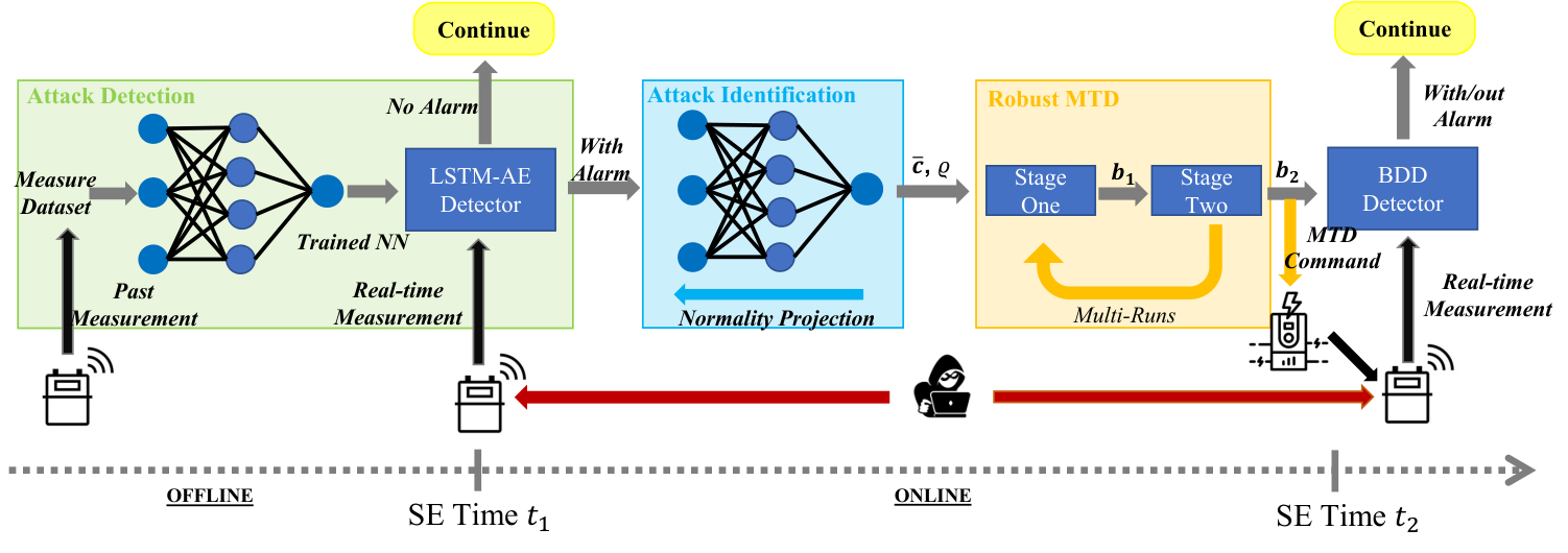
As shown in Fig. 2, the proposed DDET-MTD has three successive components in one execution cycle. First, the LSTM-AE detector in Section II-C is trained on the normal dataset offline and then tests the sensor measurement collected from SCADA in real-time operation. If a positive alarm is raised at the SE time , an attack identification algorithm is implemented to approximately extract the attack vector in the second component using the same neural network. The attack identification serves as the bridge between the data and physics by applying the extracted attack knowledge to the MTD design, in the meantime, reduces the execution cost of MTD and improves its hiddenness. In the last component, based on the identified attack, a robust MTD algorithm is triggered to verify the positive alarm from the LSTM-AE detector at the next SE time . Intuitively, the false alarms from the data-driven detector can be sufficiently rejected by the subsequent MTD due to the controllable FPR of MTD.
III-A Physics-Informed Attack Identification
The LSTM-AE detector defines a manifold for normal measurement. Therefore, the attack identification can be achieved by first recovering the normal measurement toward the manifold of the LSTM-AE detector. Following Section II-C, given a continuous measurement set with positive alarm by the LSTM-AE detector, we assume that only the last measurement vector is anomalous. Let the anomalous attack and recovered measurement be and , respectively. To explicitly encode the measurement equation (1), the recovered measurement can be written as
| (6) |
where and are the recovered real and imaginary voltage vectors. Here, the rectangular form on complex number is used to ensure stable back-propagation in Neural Network. Let . An energy function measuring the distance from to the normality manifold defined by the LSTM-AE can be written as:
| (7) | ||||
Eq. (7) can be viewed as a non-linear Lasso regression on decision variable where the projection of the attack measurement on the manifold of LSTM-AE is calculated with physical information (6) considered. In detail, the first term in (7) is the reconstruction loss (5) of the recovered normal measurement , while the second and third terms penalise the difference between real and imaginary-part voltage deviations with weights and , respectively. Since the attack is usually sparse, the -norm is used to regularise the number of attacked states. The -norm is also less sensitive to attack vector than the -norm used in of (5).

The attack identification algorithm is illustrated in Fig. 3 and Algorithm 1. As shown in Fig. 3, the physics information is encoded through the measurement equation (1) and the SE (3) when projecting the attack measurement onto the normal manifold defined by the LSTM-AE detector. Therefore, the main component of Algorithm 1 is to recover seen by both the BDD and the LSTM-AE detector. In line 3, the state estimation of the previous measurement is used as the warm start. Adam Optimiser [32] is used to minimise the weighted loss (7) by backpropagation with step size . Iteration in lines 5-14 is terminated if the reconstruction loss (5) is lower than the threshold or the maximum iteration number is achieved. The minimum iteration number is designed for warm-up purposes. Finally, the attack vector is identified by subtraction in line 15.
Given the -th attack in an attack index set , the attack identification uncertainty set can be empirically determined as where is the empirical upper bound on the deviation between the identified attack vector and the ground truth for any .
To sum up, Algorithm 1 guarantees that the recovered measurement can bypass the LSTM-AE detector and BDD. Therefore, the recovered state obeys the physics rules of power system. It also takes advantage of the formulation on FDI attacks so that the identified attack vector can lead to a stealthy attack, which further improves the identification accuracy.
III-B Hidden and Effective MTD Algorithm
In the third component of DDET-MTD, the positive alarm from the LSTM-AE detector and the identified state attack vector can be used to trigger and design the MTD algorithm. Before introducing the idea of event triggering, the MTD algorithm is formulated as follows.
| (Attacker can detect the MTD) | (8a) | |||
| subject to | (Operator can detect the attack) | (8b) | ||
Although the hiddenness of MTD is essential to deceive the prudent attacker, we argue that the main target of MTD is to detect the ongoing attack with high detection rate. Therefore, (8) is designed to minimize the attacker’s chances to notice the existence of MTD, subject to a specific detection accuracy on the attack. However, this optimisation problem is intrinsically hard to solve for two reasons. First, both the cost and the constraint in (8) are probabilistic and nonconvex, so the convergence property and global optimality are difficult to guarantee. Second, to guarantee the detection accuracy, it requires the exact knowledge of the attack vector, which cannot be known in advance. To address the first problem, local linearisations are introduced in the measurement equation (1) on which convex relaxation is applied. For the second, a robust two-stage optimisation problem is established based on the set of identification uncertainty set from Algorithm 1.
III-B1 Approximations of MTD Hiddenness
By explicitly considering the influence of susceptance on the measurement, the measurement equation (1) can be rewritten as . Under normal operation (no attack and MTD), the last iteration of SE is to solve the following normal equation:
| (9) |
where and is the state estimated before MTD. For the above system, the residual can be derived
| (10) |
where . also follows the distribution with DoF .
When the MTD is triggered, both and will be deviated from the stationary point. The first-order Taylor expansion around is written as:
| (11) |
where .
Combining (9)-(11), the attacker’s residual on the post-MTD measurement becomes:
in which the second equality is due to the fact that . Meanwhile, follows the non-central distribution (NCX) with non-centrality parameter:
| (12) |
Since the probability that the MTD is detected by the attacker increases monotonically as increases [16], should be minimised. This result is coherent to the findings in [19, 17, 14] where the measurement change before and after MTD should be small. Note that both and are constants for a given load condition. Meanwhile, can be derived analytically using similar methods in [33].
III-B2 Approximation of MTD Effectiveness
To accelerate the convergence speed and performance of SE, dishonest SE is widely used, in which the Jacobian matrix remains unchanged throughout the iteration [10]. The last iteration of dishonest SE on is represented as:
| (13) |
where is the estimated state of and .
The residual of the above system is derived as where . Similarly, follows the distribution with DoF .
When an attack exists, where is the estimated state from the attacker after the MTD is triggered. As required by the MTD hiddenness, the difference in pre- and post-MTD measurements is minimised. Therefore, it is reasonable to assume that is close to . Following Assumption Two, for small state injection, the attack vector can be approximated as [34]. Consequently, the non-centrality parameter of the post-MTD measurement under attack is approximated as:
| (14) |
III-B3 Attack-Aware Robust MTD Reformulation
Based on the approximations of the hiddenness (12) and effectiveness (14) of MTD, the probabilistic optimisation problem (8) becomes nonprobabilistic for a given attack :
| (15a) | ||||
| s.t. | (15b) | |||
In (15a), only when , the MTD can be 100% hidden to the attacker. In most of the cases, the MTD hiddenness and effectiveness are proved to be contradictory [17, 18, 19]. In (15b), the probability constraint (8b) is converted non-probabilistic. In fact, there is a such that the detection rate at is equal to [16]:
| (16) |
where represents the density function of the NCX distribution with DoF and the non-centrality parameter equals .
The optimisation (15) still requires exact knowledge of the attack vector , which is not available for the operator. Therefore, a robust reformulation of (15) is derived by guaranteeing the lowest detection rate for the attacks in the attack uncertainty set defined in Section III-A:
| (17a) | ||||
| s.t. | (17b) | |||
| (17c) | ||||
Problem (17) is a bilevel optimization problem [35]. The objective of the upper level is to decrease the chance that the attacker detects MTD. The decision variable in upper level is the MTD setpoint and the constraint on is the permissible set of D-FACTS devices . At the lower level, the objective function is to find the state injection that results in the lowest detection rate, subject to the set of uncertainties . Note that the upper level decision variable is nested at the lower level parametrically. The nesting structure robustly ensures that all possible attacks in can be detected with predefined probability .
To simplify the analysis, only active power flow measurements are considered for MTD effectiveness, as active power is more important in state estimation and sensitive to changes in the voltage phase angle[36]. As a result, the Jacobian matrix in (13) can be analytically written as:
| (18) |
where ; ; ; ; and . is the reduced incidence matrix by removing the column that represents the reference bus from the incidence matrix ; is the vector of the transformer tap ratio. The detection threshold corresponding to the active power flow measurements is denoted as . Intuitively, guaranteeing the detection rate on a subset of the measurement can also guarantee the detection rate on the full measurement due to the increased redundancy.
As proved by [16], only when the attack strength is greater than a certain threshold can be satisfied. Therefore, despite the non-linearity and non-convexity, (17) may not have a feasible solution. As a result, (17) is separated into two stages. In stage one, the feasibility of constraint (17c) is checked by maximizing its left hand side. The optimal solution of stage one is then used as the feasible warm start in stage two to improve its hiddenness.
III-B4 Convex Stage-One Optimisation
In stage one, the feasibility of constraint (17c) is checked by maximizing the detection rate on the worst-case attack in
| (19) |
Multi-run strategy is required to solve the non-convex problem (19) with different starting points in . For each run, an equivalent convex reformulation is derived as follows:
Proposition 1.
Define auxiliary variable , , , and . The problem (19) is equivalent to the following:
| (20a) | ||||
| s.t. | (20b) | |||
| (20c) | ||||
| (20d) | ||||
Proof.
The proof can be found in Appendix 0.-B. ∎
Referring to (18), the only nonlinearity of (20) is in the last block-diagonal entry of (20d). To linearise , iterative algorithm is designed with starting point and the following proposition is derived:
Proposition 2.
Let and . Define as the feasible solution of the -th iteration. A sufficient convex condition for (20d) is
| (21) |
with .
Proof.
The proof can be found in Appendix 0.-C. ∎
III-B5 Convex Stage-Two Optimisation
The stage-one problem checks the feasibility of (17c). In detail, if the optimal solution of (20) (or similarly the final iteration of (22)) is greater than , the original bilevel problem (17) can be solved with the optimal point of (20) as a feasible warm start. Otherwise, the threshold in (17c) should be reduced to to have a feasible solution. In either situation, denoting the threshold of constraint (17c) after stage one as , the following proposition gives a feasible and convex reformulation to (17) in which the MTD effectiveness is guaranteed to the level determined by stage one while the hiddenness is improved.
Proposition 3.
Proof.
The proof can be found in Appendix 0.-D. ∎
Similarly, the non-convexity in can be solved iteratively by the sufficient condition described in Proposition 2. This results in an iterative algorithm to solve the stage-two problem:
To conclude, the two-stage optimisation in DDET-MTD has been developed to guarantee the effectiveness of MTD while improving hiddenness. Based on convex relaxation, the hidden and effective MTD can be designed as follows:
- 1.
Solve the stage-one problem (22) iteratively with different start point . Store the multi-run results of in a set and the corresponding cost into a set .
- 2.
If the largest cost in is smaller than , use the corresponding susceptance in as a warm start in stage-two problem (24) and solve it iteratively.
- 3.
If the largest cost in is larger than or equal to , define the index set and candidate warm-start susceptance set . For each , iteratively solve stage-two problem (24). The optimal susceptance is returned with the smallest cost.
The detailed algorithm can be found in Appendix 0.-E.
IV Simulations and Results
IV-A Simulation Settings
IV-A1 Model Configurations
The proposed DDET-MTD algorithm is tested on the IEEE case-14 system [28]. Although we have derived the theoretical analysis using simplified models, all the simulations are implemented under full AC condition. Real-time load consumptions and photovoltaic generations are assigned to each bus for four months using a similar method in [37]. The load data is interpolated to 5-min resolution, resulting in over 35k data in total. For each operation instance, AC-OPF is solved by PyPower [28]. The standard deviation of the measurement noise is set to 2% of the default values in the case-14 system case file. The FPR of BDD is set as . The MTD threshold and are determined by (16) with . LSTM-AE attack detection and identification algorithms are trained and implemented using PyTorch[38] with hyperparameters summarised in Table II. The data set is separated into 60% training, 20% validation, and 20% test sets. Throughout the simulation, random sparse AC-FDI attacks are generated with the number of attacked buses equal to 1-3, and the strength of the attacks is set as and of the normal state solved from the real-time measurements. For example, the pair means that there are two buses being attacked with strength at random in . In the simulation, 200 attacks are randomly generated from the entire test set for each type of attack. Without losing generality, all the branches are equipped with D-FACTS devices and the maximum reactance perturbation ratio is 50% [13]. In addition, the convex MTD optimisation problems are solved by CVXPY[39] with MOSEK solver. Hyperparameters for stage-one and stage-two optimisations are summarised in Table III.
| Sample Length | 6 | Encoder Size | 68-48-29-10 |
| Epochs No. | 1000 | Batch Size | 32 |
| 0.001 | 0.005 | ||
| Early Stop Patience | 10 | Early Stop Diff. | 0 |
| 0.1 | Optimizer | Adam | |
| 1000 | 50 |
| Multi-Run No. | 15 |
|---|---|
| Max. iteration No. | 100 |
| Tolerance of stage one | 0.1 |
| Tolerance of stage two | 1 |
IV-A2 Baseline Algorithms
Two algorithms, namely, the modified Max-Rank MTD [9, 11, 10] and (incomplete) Robust MTD [16], are implemented for benchmarking the proposed algorithm. In Max-Rank MTD, the D-FACTS devices are perturbed within (with ) so that the rank of the composite matrix is maximised, which results in maximum detection rate under noiseless assumption. Due to the randomness of this algorithm, we simulate 1000 attacks for each attack scenario under different load conditions and record the average performance. The Robust MTD algorithm considers maximising the detection rate on the worst-case attack without any prior knowledge on the attack. Therefore, it can be viewed as a conservative formulation on DDET-MTD with an attack uncertainty set . Although both baseline algorithms are periodic with SE, we also simulate their event-triggering variants.
IV-A3 Metrics
Four metrics are considered throughout the simulation.
From an attack defence perspective, Attack Detection Probability (ADP) and Defence Hiddenness Probability (DHP) can be used to evaluate the effectiveness and hiddenness of MTD as follows [19].
| (25a) | |||
| (25b) |
From an economical perspective, the average cost increase and the average reactance perturbation ratio due to the trigger of MTD are considered.
IV-B LSTM-AE Detector
Fig. 4 illustrates the TPR and FPR of the LSTM-AE detector. Various detection thresholds s are determined by the distribution of reconstruction losses in the validation set [24]. As shown in Fig. 4(a), the same detection threshold based on the FPR in the validation set can result in a higher FPR in the test set due to unseen load and PV patterns. The ROC curves on different types of attack are also summarised in Fig. 4(b), which clearly shows the trade-off between TPR and FPR. In detail, larger attack results in higher detection rate and to have 90% TPRs on all types of attack, at least 25% normal operation samples are incorrectly classified as attack. Since attack is rare in real-time operation, this high FPR can significantly influence the normal operation. In the following simulation, corresponding to 8.0% FPR in the validation set is used as the detection threshold in the LSTM-AE detector, resulting in 12.84% FPR in the test set (highlighted by the red dotted line in Fig. 4).
IV-C LSTM-AE Identifier
Fig. 5 summarised the performance of the attack identification algorithm. As shown in Fig. 5(a), the average identification deviation is around 0.01p.u. and most of them are smaller than 0.04p.u.. As the average normal state angle in the simulation is 0.71p.u., the identification algorithm is accurate and stable under different attack scenarios. Fig. 5(b) tests whether the recovered measurement can bypass the BDD and LSTM-AE detector. First, since the identification algorithm filters the measurement noise by (6), the recovered measurement can certainly bypass the BDD. Second, due to the existence of regularization in the energy function (7) and the limit of iteration numbers, only 80% of the recovered measurement can bypass the LSTM-AE detector. Nonetheless, the reconstruction losses are much smaller than those of the attacked measurement, meaning that the recovered measurements are close to the normality manifold defined by the LSTM-AE detector. Therefore, the identified attack vector is quite accurate and can be used to guide the hidden and effective MTD algorithm.
IV-D Properties of DDET-MTD
In this section, we investigate the performance of the proposed DDET-MTD algorithm.
IV-D1 Sensitivity of
First, based on the identification accuracy in Fig. 5, the effectiveness and hiddenness of MTD are summarised in Fig. 6(a) and (b), respectively. In Fig. 6(a), a larger attack is more likely to be detected and, in general, ADP increases and then decreases slightly as increases. When is small, the MTD is optimised on the limited set of candidate attack vectors around the identified attack, which may not include the actual attack vector. On the contrary, when is large, the robust MTD is conservative by maximising the detection rate on the worst possible attack in a larger set, causing the actual detection rate to decrease. An extreme example is that when , a zero-state attack vector becomes the worst-case attack, leading to a trivial solution to (19). Regarding the hiddenness of MTD, Fig. 6(b) shows that MTDs on a strong attack result in high DHP, which implies the trade-off between hiddenness and effectiveness. Referring to (17), when the attack is strong, the effectiveness constraint can be more easily achieved, which in turn gives a lower residual of the attacker. Meanwhile, DHP decreases as increases, which can be explained by a similar reason. In the following, will be used as the uncertainty bound in due to its high ADP and moderate DHP.
IV-D2 Comparison with Max-Rank and Robust MTDs
In this section, Stage-One and Stage-One + Stage-Two of the proposed DDET-MTD are compared with the Max-Rank MTD and Robust MTD algorithms. To fairly verify the performance of the proposed algorithm, both Max-Rank and Robust MTDs are triggered by the same LSTM-AE detector. Therefore, only the attacks that can be detected by the LSTM-AE are evaluated by the MTD algorithms, and we will leave a full comparison in the next section. First, as shown in Fig. 7(a), both Stage-One and Stage-One + Stage-Two can achieve ADPs greater than 96% in all attack cases. The ADP of Stage-One is slightly higher than that of Stage-One + Stage-Two when the attack strength is small. This is because Stage-One maximises the residual, while Stage-Two adds the threshold as constraint. The proposed algorithm has an ADP comparable to the Robust MTD, which is significantly higher than the Max-Rank MTD. Therefore, it can be concluded that the event-triggered MTD does not significantly compromise the performance of the LSTM-AE detector shown in Fig. 4. Furthermore, Fig. 7(b) shows that adding Stage-Two can significantly improve MTD hiddenness without compromising ADP. On the contrary, without considering the hiddenness of MTD, Stage-One, Robust and Max-Rank MTDs can always be detected by the attacker once the detector raises an alarm.
IV-E Performances under Real-Time Operations
In this section, more realistic power system operation is considered. The proposed DDET-MTD is compared with the Max-Rank MTD and the Robust MTD in both periodic and event-triggering settings. Meanwhile, as cyberattacks are very rare in practise, it is reasonable to discuss MTD usage and generator cost without attacks to see how the extra defence can impact normal system operations. In addition, the false positive rate reduction of LSTM-AE detector is also discussed.
| Attack | Metric | Periodic | Event-Triggered | |||
|---|---|---|---|---|---|---|
| Max | Robust | Max | Robust | DDET | ||
| (1,0.2) | ADP | 71.90 | 90.00 | 65.10 | 74.00 | 75.50 |
| DHP | 0.00 | 0.00 | 19.20 | 23.00 | 41.24 | |
| Cost | 0.17 | 0.64 | 0.14 | 0.47 | 0.02 | |
| Reac. | 27.53 | 45.69 | 22.30 | 34.84 | 17.15 | |
| ADP | 83.40 | 93.00 | 79.70 | 84.50 | 85.50 | |
| DHP | 0.00 | 0.00 | 11.70 | 12.00 | 64.00 | |
| Cost | 0.17 | 0.61 | 0.16 | 0.54 | 0.01 | |
| Reac. | 27.73 | 45.50 | 24.12 | 40.21 | 11.01 | |
| ADP | 93.10 | 98.50 | 90.81 | 98.00 | 95.50 | |
| DHP | 0.00 | 0.00 | 2.20 | 2.00 | 34.72 | |
| Cost | 0.17 | 0.60 | 0.16 | 0.60 | 0.01 | |
| Reac. | 27.34 | 45.82 | 26.95 | 44.63 | 16.56 | |
| ADP | 96.91 | 100.00 | 98.10 | 100.00 | 100.00 | |
| DHP | 0.00 | 0.00 | 0.40 | 0.00 | 67.00 | |
| Cost | 0.17 | 0.64 | 0.17 | 0.631 | 0.00 | |
| Reac. | 27.45 | 45.63 | 23.38 | 45.54 | 9.12 | |
| ADP | 98.90 | 99.00 | 97.61 | 99.00 | 100.00 | |
| DHP | 0.00 | 0.00 | 0.80 | 1.00 | 45.00 | |
| Cost | 0.18 | 0.62 | 0.17 | 0.64 | 0.00 | |
| Reac. | 27.24 | 45.21 | 27.36 | 45.28 | 13.66 | |
| ADP | 99.80 | 100.00 | 99.90 | 100.00 | 100.00 | |
| DHP | 0.00 | 0.00 | 0.00 | 0.00 | 81.00 | |
| Cost | 0.17 | 0.66 | 0.18 | 0.65 | 0.00 | |
| Reac. | 27.53 | 45.54 | 27.57 | 45.85 | 7.33 | |
IV-E1 Operations under FDI Attack
Average performances of Max-Rank MTD (Max), Robust MTD (Robust), and DDET-MTD (DDET) under different attack scenarios are compared in Table IV.
In general, DDET-MTD has the highest DHPs under each attack. Note that the DHPs of event-triggered Max-Rank and Robust MTDs are not zero due to the missing alarms (false negative samples) from the LSTM-AE detector. The false negative rate of LSTM-AE detector also causes the lower ADP of DDET-MTD than the periodic Robust MTD when the attack strength is low (see Fig. 4(b)). However, the periodic Robust MTD is the least economical method and cannot improve the hiddenness of MTD.
Thanks to the attack uncertainty set , the DDET-MTD can detect the attack with fewer efforts, resulting in the best economic performance of the lowest average reactance perturbation. Additionally, when the attack strength increases, the reactance perturbation ratio decreases, which can save the usage of D-FACTS devices in real-time operation. In contrast, as Robust MTD considers the worst detection performance all the time, it has the worst economic performance. The Robust and Max-Rank MTDs have almost constant average ratios per D-FACTS device under both periodic and event-triggering settings, as both algorithms cannot reflect different attack strengths and can easily over-react most of the time.
Although optimisation (8) does not take the generator cost into account, simulation shows that DDET-MTD results in the lowest cost increase under each attack for two reasons. First, the DDET-MTD has the minimum reactance deviation against the default reactance settings. Therefore, its operational point is the closest to the optimal setting. Second, by improving the MTD hiddenness, the pre- and post- MTD power flows become similar to each other, resulting in less flow redistribution and similar line losses. Furthermore, Table IV also illustrates that smaller costs are needed to detect more intense attacks in DDET-MTD, which is similar to the reactance perturbation.
To better illustrate the performances, Fig. 8 calculates the ratio of ADP and DHP with respect to the average perturbation ratio. It can be demonstrated that the DDET-MTD has the best trade-off between attack defence and operation economics, especially when the attack strength is high.
IV-E2 False Positive Rejection
Fig. 9(a) records the residuals of the LSTM-AE detector in a single day from the test set. Positive samples are highlighted as red circles. There are many false positive alarms during the night, which can be caused by irregular use of electricity. Once the LSTM-AE detector raises an alarm, the attack identification and MTD will be triggered. As there is no ongoing attack, the residual of the post-MTD measurement follows the distribution. Consequently, as shown by Fig. 9(b), all the false positive samples have residuals lower than the BDD threshold and no further actions are needed by the system operator. On average, the FPR of the LSTM-AE detector is reduced from 12.84% to 1.84% on test set after applying DDET-MTD. Note that the MTD FPR is well controlled by the predetermined BDD FPR .
IV-E3 Normal Operations
We now compare the economic performances of different MTD strategies without FDI attacks. The results in Table V demonstrate that event triggering can significantly reduce the reactance perturbation and extra operational cost of MTDs. Meanwhile, the proposed DDET-MTD has the least interference with normal system operation, which makes it a promising defence against rare FDI attacks.
| Metric | Periodic | Event-Triggered | |||
|---|---|---|---|---|---|
| Max | Robust | Max | Robust | DDET | |
| Cost | 0.171 | 0.628 | 0.019 | 0.059 | 0.005 |
| Reac. | 27.470 | 45.565 | 3.159 | 5.069 | 2.334 |
V Conclusion
This paper proposes a novel Data-Driven Event-Triggered MTD algorithm to achieve high TPR and low FPR against FDI attacks, which can benefit both the data-driven detector and the physics-based MTD. Numeric simulations verify that the proposed DDET-MTD has better defence and economic trade-off compared with two baseline algorithms. On one hand, the high FPR of data-driven detector (12.8%) is reduced by the MTD with controllable FPR (1.8%) during the normal operation. During the attack, the attack identification serves as a bridge between data and physics. The roughly identified attack vector informs to design a bilevel hidden and effective MTD algorithm, which is further solved via two-stage convex relaxations. Thanks to the knowledge of the grid model, the DDET-MTD has a comparable detection accuracy as the robust MTD (96%) while improves the hiddenness by 50%. On the other hand, the inevitable extra cost of operating MTD on the physical power grid is negligible through the triggering mechanism and optimal design enabled by the data-driven detector. The proposed DDET-MTD can significantly reduce the reactance perturbation by 70%, compared to the Robust MTD.
0.-A Convert the Range of Reactance into Susceptance
Let the branch have resistance and reactance . The susceptance can be determined as:
Therefore, decreases monotonically on and increases on . Considering the permissible range of , the permissible range of can be determined. For , , ; for , , .
0.-B Proof to Proposition 1
To start, the Schur complement [40] is given as follows.
Theorem 1.
Given any symmetric matrix , if is invertible, the following two conditions are equivalent: (1) If , then ; (2) .
Proposition 4.
Given any symmetric matrix , the following two conditions are equivalent: (1) ; (2) , , .
First, the inner problem of (19) can be written as:
| (0..1) | ||||
where and the Lagrangian of (0..1) is written as:
| (0..2) |
Let . The dual problem of (0..1) becomes:
| (0..4) | ||||
Note that the last constraint of (0..4) can be rewritten as . Applying Proposition 4, the dual problem can be rewritten as
| (0..5) | ||||
0.-C Proof to Proposition 2
First, the following sufficient condition holds for any matrices with the same dimension [42]:
Define and . Replacing in (20d) by finalises the proof.
0.-D Proof to Proposition 3
The dual function (0..3) is the lower bound of the primary function, e.g. for . Therefore, a sufficient condition for (17c) is . Note that is replaced by constant in stage two. Therefore, Proposition 3 can be proved similarly to Proposition 1. Furthermore, define the cost of (17) as . Applying Theorem 1 on gives (23c).
0.-E Hidden and Effective MTD Algorithm
The hidden and effective MTD algorithm is summarised in Algorithm 2 in detail. The inputs of the algorithm , , , , , , , and have been defined in the main content. Further, define and as the tolerance of stage-one and stage-two problem, respectively. Define and as the maximum iteration step in stage-one and stage-two problem, respectively. Meanwhile, let be the multi-run number. The output of this algorithm is the set-point of the D-FATCS devices, denoted as .
References
- [1] M. S. Mahmoud, H. M. Khalid, and M. M. Hamdan, Cyberphysical Infrastructures in Power Systems: Architectures and Vulnerabilities. Academic Press, 2021.
- [2] H. M. Khalid and J. C.-H. Peng, “A bayesian algorithm to enhance the resilience of wams applications against cyber attacks,” IEEE Transactions on Smart Grid, vol. 7, no. 4, pp. 2026–2037, 2016.
- [3] G. Hug and J. A. Giampapa, “Vulnerability assessment of ac state estimation with respect to false data injection cyber-attacks,” IEEE Transactions on Smart Grid, vol. 3, no. 3, pp. 1362–1370, 2012.
- [4] R. Deng, G. Xiao, R. Lu, H. Liang, and A. V. Vasilakos, “False data injection on state estimation in power systems—attacks, impacts, and defense: A survey,” IEEE Transactions on Industrial Informatics, vol. 13, no. 2, pp. 411–423, 2017.
- [5] F. Bellizio, W. Xu, D. Qiu, Y. Ye, D. Papadaskalopoulos, J. L. Cremer, F. Teng, and G. Strbac, “Transition to digitalized paradigms for security control and decentralized electricity market,” Proceedings of the IEEE, pp. 1–18, 2022.
- [6] G. Cheng, Y. Lin, J. Zhao, and J. Yan, “A highly discriminative detector against false data injection attacks in ac state estimation,” IEEE Transactions on Smart Grid, 2022.
- [7] M. Higgins, J. Zhang, N. Zhang, and F. Teng, “Topology learning aided false data injection attack without prior topology information,” in 2021 IEEE Power Energy Society General Meeting (PESGM), 2021, pp. 1–5.
- [8] M. A. Rahman, E. Al-Shaer, and R. B. Bobba, “Moving target defense for hardening the security of the power system state estimation,” in Proceedings of the First ACM Workshop on Moving Target Defense, 2014, pp. 59–68.
- [9] C. Liu, J. Wu, C. Long, and D. Kundur, “Reactance perturbation for detecting and identifying fdi attacks in power system state estimation,” IEEE Journal of Selected Topics in Signal Processing, vol. 12, no. 4, pp. 763–776, 2018.
- [10] Z. Zhang, R. Deng, D. K. Yau, P. Cheng, and J. Chen, “Analysis of moving target defense against false data injection attacks on power grid,” IEEE Transactions on Information Forensics and Security, vol. 15, pp. 2320–2335, 2019.
- [11] B. Liu and H. Wu, “Optimal d-facts placement in moving target defense against false data injection attacks,” IEEE Transactions on Smart Grid, vol. 11, no. 5, pp. 4345–4357, 2020.
- [12] M. Higgins, W. Xu, F. Teng, and T. Parisini, “Cyber-physical risk assessment for false data injection attacks considering moving target defences,” International Journal of Information Security, 2022.
- [13] S. Lakshminarayana and D. K. Yau, “Cost-benefit analysis of moving-target defense in power grids,” IEEE Transactions on Power Systems, vol. 36, no. 2, pp. 1152–1163, 2020.
- [14] M. Liu, C. Zhao, Z. Zhang, and R. Deng, “Explicit analysis on effectiveness and hiddenness of moving target defense in ac power systems,” IEEE Transactions on Power Systems, pp. 1–1, 2022.
- [15] H. Zhang, B. Liu, X. Liu, A. Pahwa, and H. Wu, “Voltage stability constrained moving target defense against net load redistribution attacks,” IEEE Transactions on Smart Grid, vol. 13, no. 5, pp. 3748–3759, 2022.
- [16] W. Xu, I. M. Jaimoukh, and F. Teng, “Robust moving target defence against false data injection attacks in power grids,” IEEE Transactions on Information Forensics and Security, pp. 1–1, 2022.
- [17] J. Tian, R. Tan, X. Guan, and T. Liu, “Enhanced hidden moving target defense in smart grids,” IEEE transactions on smart grid, vol. 10, no. 2, pp. 2208–2223, 2018.
- [18] Z. Zhang, R. Deng, D. K. Yau, P. Cheng, and J. Chen, “On hiddenness of moving target defense against false data injection attacks on power grid,” ACM Transactions on Cyber-Physical Systems, vol. 4, no. 3, pp. 1–29, 2020.
- [19] B. Liu and H. Wu, “Optimal planning and operation of hidden moving target defense for maximal detection effectiveness,” IEEE Transactions on Smart Grid, vol. 12, no. 5, pp. 4447–4459, 2021.
- [20] M. Higgins, K. Mayes, and F. Teng, “Enhanced cyber-physical security using attack-resistant cyber nodes and event-triggered moving target defence,” IET Cyber-Physical Systems: Theory & Applications, vol. 6, no. 1, pp. 12–26, 2021.
- [21] W. Xu, I. M. Jaimoukha, and F. Teng, “Physical verification of data-driven cyberattack detector in power system: An mtd approach,” in 2022 IEEE PES Innovative Smart Grid Technologies Conference Europe (ISGT-Europe), 2022, pp. 1–5.
- [22] T. Wu, W. Xue, H. Wang, C. Y. Chung, G. Wang, J. Peng, and Q. Yang, “Extreme learning machine-based state reconstruction for automatic attack filtering in cyber physical power system,” IEEE Transactions on Industrial Informatics, vol. 17, no. 3, pp. 1892–1904, 2021.
- [23] Y. Zhang, J. Wang, and B. Chen, “Detecting false data injection attacks in smart grids: A semi-supervised deep learning approach,” IEEE Transactions on Smart Grid, vol. 12, no. 1, pp. 623–634, 2021.
- [24] W. Xu and F. Teng, “A deep learning based detection method for combined integrity-availability cyber attacks in power system,” arXiv preprint arXiv:2011.01816, 2020.
- [25] G. Pang, C. Shen, L. Cao, and A. V. D. Hengel, “Deep learning for anomaly detection: A review,” ACM Computing Surveys (CSUR), vol. 54, no. 2, pp. 1–38, 2021.
- [26] C. M. Ahmed, G. R. MR, and A. P. Mathur, “Challenges in machine learning based approaches for real-time anomaly detection in industrial control systems,” in Proceedings of the 6th ACM on Cyber-Physical System Security Workshop, 2020, pp. 23–29.
- [27] A. Ashok, M. Govindarasu, and V. Ajjarapu, “Online detection of stealthy false data injection attacks in power system state estimation,” IEEE Transactions on Smart Grid, vol. 9, no. 3, pp. 1636–1646, 2018.
- [28] R. Zimmerman and C. MurilloSanchez, “Matpower user’s manual version 7.0 b1,” Power Systems Engineering Research Center (PSerc): Tempe, AZ, USA, 2018.
- [29] A. Abur and A. G. Exposito, Power system state estimation: theory and implementation. CRC press, 2004.
- [30] H. Zhang, B. Liu, and H. Wu, “Smart grid cyber-physical attack and defense: A review,” IEEE Access, vol. 9, pp. 29 641–29 659, 2021.
- [31] S. Gao, J. Lei, X. Wei, Y. Liu, and T. Wang, “A novel bilevel false data injection attack model based on pre-and post-dispatch,” IEEE Transactions on Smart Grid, pp. 1–1, 2022.
- [32] D. P. Kingma and J. Ba, “Adam: A method for stochastic optimization,” arXiv preprint arXiv:1412.6980, 2014.
- [33] B. Liu, Q. Yang, H. Zhang, and H. Wu, “An interior-point solver for ac optimal power flow considering variable impedance-based facts devices,” IEEE Access, vol. 9, pp. 154 460–154 470, 2021.
- [34] C. Liu, H. Liang, T. Chen, J. Wu, and C. Long, “Joint admittance perturbation and meter protection for mitigating stealthy fdi attacks against power system state estimation,” IEEE Transactions on Power Systems, vol. 35, no. 2, pp. 1468–1478, 2019.
- [35] A. Sinha, P. Malo, and K. Deb, “A review on bilevel optimization: from classical to evolutionary approaches and applications,” IEEE Transactions on Evolutionary Computation, vol. 22, no. 2, pp. 276–295, 2017.
- [36] C. Liu, R. Deng, W. He, H. Liang, and W. Du, “Optimal coding schemes for detecting false data injection attacks in power system state estimation,” IEEE Transactions on Smart Grid, vol. 13, no. 1, pp. 738–749, 2021.
- [37] J. Wang, W. Xu, Y. Gu, W. Song, and T. Green, “Multi-agent reinforcement learning for active voltage control on power distribution networks,” Advances in Neural Information Processing Systems, vol. 34, 2021.
- [38] A. Paszke, S. Gross, F. Massa, A. Lerer, J. Bradbury, G. Chanan, T. Killeen, Z. Lin, N. Gimelshein, L. Antiga et al., “Pytorch: An imperative style, high-performance deep learning library,” Advances in neural information processing systems, vol. 32, 2019.
- [39] S. Diamond and S. Boyd, “CVXPY: A Python-embedded modeling language for convex optimization,” Journal of Machine Learning Research, vol. 17, no. 83, pp. 1–5, 2016.
- [40] J. H. Gallier. (2010) Notes on the schur complement. [Online]. Available: https://repository.upenn.edu/cgi/viewcontent.cgi?article=1637&context=cis_papers
- [41] S. Boyd and L. Vandenberghe, Convex optimization. Cambridge university press, 2004.
- [42] C. Liu and I. M. Jaimoukha, “The computation of full-complexity polytopic robust control invariant sets,” in 2015 54th IEEE Conference on Decision and Control (CDC), 2015, pp. 6233–6238.
![[Uncaptioned image]](2204.12970v2/bio_photo/WangkunXu.jpg) |
Wangkun Xu (Student Member, IEEE) received B.Eng. degree in electrical and electronic engineering from University of Liverpool, UK in 2018 and M.Sc. degree in control systems from Imperial College London, UK in 2019, where he is currently a Ph.D. student. His research focuses on robust and privacy-preserving machine learnings in cyber-physical power system operation and security. |
![[Uncaptioned image]](2204.12970v2/bio_photo/MartinHiggins.jpg) |
Martin Higgins (Member, IEEE) received his BSc in Physics from Queen Mary, University of London, in 2011 and his MSc and Ph.D. from Imperial College London, U.K. in 2012 and 2022 respectively. His Ph.D. thesis was on False Data Injection attacks against power systems and was achieved as part of the CDT in Smart Grids integrated MRES/PHD. Currently, Martin is a research associate at the University of Oxford contributing on the Digital Security by Design Project. His research interests include power systems cyber-security, self-driving vehicles, sensor spoofing attacks, false data injection attacks and moving target defence. |
![[Uncaptioned image]](2204.12970v2/bio_photo/JianhongWang.jpeg) |
Jianhong Wang received B.Eng. degree in Computer Science and Electronic Engineering from University of Liverpool, UK in 2016, M.Sc. degree in Computing (Machine Learning) from Imperial College London, UK in 2017, and M.Res. degree in Web Science and Data Analytics from University College London, UK in 2018. He is currently pursuing the Ph.D. degree in Electrical Engineering Research at Imperial College London, UK. His research interests lie in multi-agent reinforcement learning and its applications to the real-world problems. He has published several papers in AI top conferences such as AAAI, NeurIPS and ICLR. |
![[Uncaptioned image]](2204.12970v2/bio_photo/ImadJaimoukha.jpg) |
Imad M. Jaimoukha received the B.Sc. degree in electrical engineering from the University of Southampton, Southampton, U.K., in 1983, and the M.Sc. and Ph.D. degrees in control systems from Imperial College London, London, U.K., in 1986 and 1990, respectively. He was a Research Fellow with the Centre for Process Systems Engineering at ICL from 1990 to 1994. Since 1994, he has been with the Department of Electrical and Electronic Engineering, ICL. His research interests include robust and fault-tolerant control, system approximation, and global optimization. |
![[Uncaptioned image]](2204.12970v2/bio_photo/FeiTeng.png) |
Fei Teng (Senior Member, IEEE) received the B.Eng. degree in electrical engineering from Beihang University, China, in 2009, and the M.Sc. and Ph.D. degrees in electrical engineering from Imperial College London, U.K., in 2010 and 2015, respectively, where he is currently a Senior Lecturer with the Department of Electrical and Electronic Engineering. His research focuses on the power system operation with high penetration of Inverter-Based Resources (IBRs) and the Cyber-resilient and Privacy-preserving cyber-physical power grid. |