P. Faliszewski, V. Mascardi, C. Pelachaud, M.E. Taylor (eds.)

Learning to Transfer Role Assignment Across Team SizesConference: Proc.of the 21st International Conference on Autonomous Agents and Multiagent Systems (AAMAS 2022); May 9–13, 2022; Online439

Dung Nguyen Affiliation: A²I², Deakin University , Geelong , Australia email: dung.nguyen@deakin.edu.au , Phuoc Nguyen Affiliation: A²I², Deakin University , Geelong , Australia email: phuoc.nguyen@deakin.edu.au , Svetha Venkatesh Affiliation: A²I², Deakin University , Geelong , Australia email: svetha.venkatesh@deakin.edu.au and Truyen Tran Affiliation: A²I², Deakin University , Geelong , Australia email: truyen.tran@deakin.edu.au

2022© , 2022;

Abstract.

Multi-agent reinforcement learning holds the key for solving complex tasks that demand the coordination of learning agents. However, strong coordination often leads to expensive exploration over the exponentially large state-action space. A powerful approach is to decompose team works into roles, which are ideally assigned to agents with the relevant skills. Training agents to adaptively choose and play emerging roles in a team thus allows the team to scale to complex tasks and quickly adapt to changing environments. These promises, however, have not been fully realised by current role-based multi-agent reinforcement learning methods as they assume either a pre-defined role structure or a fixed team size. We propose a framework to learn role assignment and transfer across team sizes. In particular, we train a role assignment network for small teams by demonstration and transfer the network to larger teams, which continue to learn through interaction with the environment. We demonstrate that re-using the role-based credit assignment structure can foster the learning process of larger reinforcement learning teams to achieve tasks requiring different roles. Our proposal outperforms competing techniques in enriched role-enforcing Prey-Predator games and in new scenarios in the StarCraft II Micro-Management benchmark.

Keywords:

Multi-agent Reinforcement Learning; Centralised Training Decentralised Execution; Roles; SMAC

1. Introduction

Learning to work as a team is essential to achieve larger collective goals in solving complex tasks Buşoniu et al. 2010; Zhang et al. 2021. However, partial observations and expensive team coordination may prevent agents from having full knowledge of the environment and all others operating on it Omidshafiei et al. 2017; Wang et al. 2021a. Early work avoided this difficulty by learning independent single-agent policies and treating other learning agents as part of the environment Matignon et al. 2012; Tan 1993, but may run into the non-stationary problem Wang et al. 2021a. Centralised Training Decentralised Execution (CTDE) Rashid et al. 2018; Oliehoek et al. 2008; Kraemer and Banerjee 2016 is a middle ground assuming that the agents act on their own after being trained together. The essence of CTDE is to learn to assign credit to individual agents when the whole team is trained to maximise collective rewards. There has been a growing effort to solve CTDE Mahajan et al. 2019; Rashid et al. 2018; Wang et al. 2020a; Lowe et al. 2017; Foerster et al. 2018; Gupta et al. 2017, but these are typically limited to small teams of agents since it is prohibitive to explore the joint state-action space of large teams during training. Learning with a large number of agents remains very challenging Samvelyan et al. 2019b; Wang et al. 2021a.

Refer to caption — Figure 1. A StarCraft II scenario in which the agents need to play different roles to explore good policies. Some marines need to defend own campsites (bottom) under attack, enabling their allies to attack the opponent’s campsites (top).

A solution found to be effective in human teams is to decompose a large team task into sub-tasks and roles. Under this decomposition, each team member assumes one or more roles associated with manageable sub-tasks Biddle 2013. Training a large team is therefore feasible as each individual needs to explore only a constrained state-action space defined by the assigned roles. However, in practice, the role structures are not always well-defined a priori or are changing due to the task or team dynamics. In these circumstances, members need to assume emerging roles and proactively play the chosen roles when they see fit Wang et al. 2020a. Learning to play emergent roles essentially boils down to how to assign credits to roles followed by assignments to the agents who play the roles Wang et al. 2021a.

An orthogonal approach in solving difficult tasks is to learn with a curriculum in that we start from a small, easy-to-learn task, then progressively expand the reach to larger tasks Elman 1993; Narvekar and Stone 2019; Narvekar et al. 2020. For example, it would be learning from a small, simple environment first, and gradually training in larger, more complex environments. In multi-agent settings, it could be progressing from training a small team where coordination is easy and cheap, then transferring the learned skills to the next phase of training with a larger team where coordination is difficult and expensive Wang et al. 2020b. This curriculum strategy demands a new kind of models that can work across team sizes.

In this work, we seek to bring these two approaches into a unified learning framework for CTDE, which consists of (a) team learning to assign credit to roles, and (b) transferring models (both credit assignment and individual policy) across varying team sizes. We start from a popular CTDE framework known as QMIX Rashid et al. 2018, which has a mixing network to aggregate $Q$ -value functions of individual agents into the team’s $Q$ -value function. The mixing network is generated by a hyper-network Ha et al. 2017 that takes as input the state, and thus assuming a fixed team size. Lifting this constraint, we design a new mixing network and a new way to generate the network from observations local to each agent rather than from the entire state of the system. The design of the mixing network permits (a) dynamic credit assignments to hidden roles, and (b) role assignments to individual agents. At each time step, the network estimates the probability that an agent will contribute to a role, collects the $Q$ -function values attributed to the role, and weights the role’s contribution to the total team’s $Q$ -function. Crucially, our generating hyper-network is transferable across teams by permitting varying team sizes to borrow pre-trained models. This enables faster training in a new setting and curriculum learning from easy to complex scenarios.

To further encourage the role differentiation and assignment among agents, we introduce role-induced losses. For concreteness, we study a loss associated with the reward horizons, as encapsulated in the discount factors in the MDP. This is motivated by the fact that we humans engage in playing a long-term rewarded role for the whole team even when we know the role has no short-term individual benefit. We evaluate our proposed framework on two suites of multi-agent reinforcement learning (MARL) experiments, highlighting the need for curriculum learning when solving strongly cooperative CTDE tasks. The first suite consists of enriched Prey-Predator games, where agents must learn to recognise, pick and play an emergent role for the team to succeed. Visual examination clearly shows that (a) the roles emerge, and (b) curriculum learning enabled by transferring role assignment is critical to success in larger teams. The other suite of experiments is derived from the popular StarCraft Multi-agent challenge (SMAC) Samvelyan et al. 2019a where we enforce stricter team coordination. Again we demonstrate that ours converges much faster than competing methods when tested on larger teams, thanks to the ability to transfer role assignment from smaller teams.

To summarise, our contributions are: (1) A neural framework that learns to assign credits and agents to roles, and supports transferring across different team sizes. The latter further enables curriculum learning to succeed in larger team settings and more complex tasks; and (2) An enriched version of Prey-Predator games and a suite of new scenarios in SMAC to support varying reward horizons.

2. Preliminaries

Cooperative Reinforcement Learning Agents

We consider a fully cooperative multi-agent task described as a decentralised Partial Observability Markov Decision Process (Dec-POMDP) Oliehoek and Amato 2016 $G=\left\langle\mathcal{N},\mathcal{S},\mathcal{A},\mathcal{P},R,\Omega,\mathcal{O},\gamma\right\rangle$ in which $\mathcal{N}$ is the set of agents, $s\in\mathcal{S}$ is the true state of the environment, $\mathcal{O}$ is the observation space, $\mathcal{A}$ is the action space, $\Omega:\mathcal{S}\longmapsto\mathcal{O}$ is a mapping from state space to the observation space, $\mathcal{P}:\mathcal{S}\times\mathcal{A}^{|\mathcal{N}|}\times\mathcal{S}\longmapsto\left[0,1\right]$ is the state transition function, $R:\mathcal{S}\times\mathcal{A}^{|\mathcal{N}|}\longmapsto\mathbb{R}$ is the reward function, and $\gamma\in\left[0,1\right]$ is the discounted factor. At each time step $t$ , an agent $i$ observes its local observation $o_{i}^{(t)}\in\mathcal{O}$ then decides its action $a_{i}^{(t)}\in\mathcal{A}$ . All agents in the environment form a joint-action $a\in\mathcal{A}^{|\mathcal{N}|}$ .

Centralised Training and Decentralised Execution (CTDE)

In this setting, we train a team of agents together to maximise team rewards resulting from individuals executing their own policies $\pi^{i}:\mathcal{O}\longmapsto\mathcal{A}$ with $i\in\mathcal{N}$ . Once trained, agents make decisions based on their own local observations. The CTDE scheme allows the team of agents to know the true state of the environment $s\in\mathcal{S}$ and all observations of others $o_{j}\in\mathcal{O}$ for all $j\in\mathcal{N}$ during training. Howerver, an agent can only access to its local observations $o_{i}^{(t)}$ to make decision $a_{i}^{(t)}$ during execution to maximise the team reward $R_{\text{team}}=\sum_{i\in\mathcal{N}}\sum_{t=0}^{T}\gamma^{t}r_{i}^{(t)}$ .

3. Proposed Method

Under the CTDE scheme, our aim is to design an architecture that learns to factorise the total value function of the team $Q^{tot}(s,\boldsymbol{a})$ into $N=|\mathcal{N}|$ components, i.e. each agent $i$ will predict a value $Q_{i}(o_{i},a_{i})$ based on its local observation $o_{i}$ and action $a_{i}$ . That is, $Q^{tot}$ is a mixing function, computed by the mixing network whose input is the variable-size set of mixed values $\mathbf{Q}=\left\{Q_{1},Q_{2},...,Q_{N}\right\}$ . The challenge is in learning the mixing network to properly assign credits to individual agents who play the emerging roles as the team interacts with the environment. The overall network design is given in Fig. 2.

Each value function $Q_{i}$ is computed using a recurrent neural network that takes the current observation, its own execution trajectory, and a possible action. Given the local observation $o_{i}^{(t)}$ at time step $t$ , the agent $i$ computes its prediction of action-value $Q_{i}(o_{i}^{(t)},a_{i}^{(t)})=\text{MLP}\left(h_{i}^{(t)}\right)$ where $x_{i}^{(t)}=\text{ReLU}\left(\text{MLP}(o_{i}^{(t)})\right)$ is a transformation of the observation and $h_{i}^{(t)}=\text{GRU}\left(x_{i}^{(t)},h_{i}^{(t-1)}\right)$ is the hidden states of the gated recurrent neural networks (GRU) Chung et al. 2014.

3.1. The Mixing Network

Taking the role-based approach and assuming there are $K$ “roles”, we design a new neural architecture for the mixing network. Given the prediction of individual agents $\left\{Q_{i}\right\}_{i=1}^{N}$ , the mixing network makes a prediction about the team reward:

(1)		$\displaystyle Q^{tot}$	$\displaystyle=b^{(2)}+\sum_{k=1}^{K}\mathbf{W}_{k}^{(2)}\sigma\left(\mathbf{b}_{k}^{(1)}+\sum_{i=1}^{N}\mathbf{W}_{ik}^{(1)}Q_{i}\right),\,\text{s.t.}$
(2)		$\displaystyle\mathbf{W}_{ik}^{(1)}$	$\displaystyle\geq 0;\,\,\sum_{i}\mathbf{W}_{ik}^{(1)}=1;\,\,\text{and}\,\mathbf{W}_{k}^{(2)}\geq 0\,\,\text{for all}\,i,k,$

where $\left\{\mathbf{W}^{(1)},\mathbf{W}^{(2)}\right\}$ are mixing coefficients, $\left\{\mathbf{b}^{(1)},b^{(2)}\right\}$ are biases, and $\sigma(\cdot)$ is an activation function chosen to be Exponential Linear Unit in our implementation.

The mixing coefficient $\mathbf{W}_{ik}^{(1)}$ measures the contribution of each agent $i$ to a role $k$ . The normalisation over agents $\sum_{i}\mathbf{W}_{ik}^{(1)}=1$ for all $k$ can be interpreted as the probabilities we use to select the agents for each role. The mixing coefficient $\mathbf{W}_{k}^{(2)}$ assigns the credit to a role $k$ in the total estimated reward.

The mixing function in Eq. (1) was first studied in QMIX Rashid et al. 2018 in that the mixing coefficients and biases are state-dependent, i.e., through hyper-networks (e.g., see Ha et al. 2017) or fast weight (e.g., see Hinton and Plaut 1987; Schmidhuber 1992). However, as QMIX uses the global information (state) to compute $\mathbf{W}^{(1)}$ , it must assume a fixed team size without role assignment, and thus cannot transfer the mixing network across different team sizes with different roles.

To tackle this drawback, we design the hyper-network of the first layer such as it receives the local observations of the agents as inputs instead of the global states. The hyper-network generates the mixing coefficients as follows:

\mathbf{W}_{i}^{(1)}=\text{softmax}_{i}\left(\mathbf{U}_{2}\sigma\left(\mathbf{U}_{1}o_{i}^{(t)}\right)\right),

where $o_{i}^{(t)}\in\mathbb{R}^{D}$ is the observation vector of the agent $i$ , $\mathbf{U}_{1}\in\mathbb{R}^{H\times D}$ and $\mathbf{U}_{2}\in\mathbb{R}^{K\times H}$ are the weights. Other mixing coefficients and biases are computed similarly to those in QMIX: $\mathbf{b}_{1}^{(1)}=\text{MLP}\left(s^{(t)}\right)$ ; $b^{(2)}=\text{MLP}\left(\sigma\left(\text{MLP}\left(s^{(t)}\right)\right)\right)$ and $\mathbf{W}^{(2)}=\text{MLP}\left(\sigma\left(\text{MLP}\left(s^{(t)}\right)\right)\right)$ .

Remark

Our architecture enables the ability to transfer the mixing networks across different team sizes. Therefore, this helps train a team to solve difficult tasks with a smaller number of samples, even in situations that could not be solved by QMIX.

3.2. Role-Specific Reward Horizons

The effective time horizon for an action is often encapsulated in the discount factor $\gamma$ of the expected future rewards. However, specifying the discount factor remains an art. We hypothesise that, in general, roles are best played with a given time horizon: some roles are biased towards immediate rewards (e.g., shooting prey in sight), while others are gearing towards the long-term (e.g., guarding the camp).

This suggests the following regulariser at each time step $t$ of a training episode:

(3)

\mathcal{R}_{LSTRR}^{(t)}=\frac{1}{K_{2}}\sum_{k=1}^{K_{2}}\left(Q_{k}^{*}-R_{k}\right)^{2}\,\,\text{for\,}\,K_{2}\leq K,

where LSTRR stands for Long-Short Term Rewarded Roles. Here $Q_{k}^{*}=\sigma\left(\sum_{i\in\mathcal{N}}\mathbf{W}_{ik}^{(1)}Q_{i}+b_{k}^{(1)}\right)$ is an estimation of the $Q$ -value associated with role $k$ , and $R_{k}=\sum_{\tau=0}^{T-t}\gamma_{k}^{\tau}r^{(t+\tau)}$ is the discounted reward for role $k$ . This regulariser is used during the centralised training process while we know the rewards. Without loss of generality we assume $\gamma_{1},\gamma_{2},...,\gamma_{K_{2}}$ is a decreasing sequence (from long-term to short-term horizons). In practice, we choose $K_{2}=\left\lceil\frac{K}{2}\right\rceil$ to compute the summation of all $Q_{k}^{*}$ ( $k\in\left[1,K_{2}\right],k\in\mathbb{N}$ ) before concatenating to $K-K_{2}$ components and multiplying with $\mathbf{W}_{k}^{(2)}$ for $k\in\left[1,K-K_{2}+1\right],k\in\mathbb{N}$ .

3.3. Scaling Team Sizes by Curriculum Learning

It has been observed that training a large team in CTDE is difficult Samvelyan et al. 2019b; Wang et al. 2021a. Thus we propose curriculum-based learning. We start by training a small team then transfer to larger teams, thus effectively reusing learnt models. Transferring across team sizes is possible thanks to the design of the mixer which takes as input agent-specific observations instead of the full observation of the whole team.

Training a smaller team permits learning by demonstrations from experts. Thus, it suggests a two-phase training procedure: (i) pre-train a small team on experiences from experts using a supervised loss $\mathcal{L}_{sup}^{(t)}$ , and (ii) continue to train on a larger team through interacting with the environment using a the temporal difference (TD) loss $\mathcal{L}_{TD}^{(t)}$ . Both steps can be expressed in the following joint loss function:

(4)

\mathcal{L}^{(t)}=\mathcal{L}_{TD}^{(t)}+\lambda_{1}\mathcal{L}_{sup}^{(t)}+\lambda_{2}\mathcal{R}_{LSTRR}^{(t)},

where $\lambda_{1}>0$ is the contributing factor of the demonstration when possible, and $\lambda_{2}>0$ is the contributing factor of the horizon regularisation defined in Eq. (3) when the reward horizon matter. The losses are defined as:

	$\displaystyle\mathcal{L}_{sup}^{(t)}$	$\displaystyle=-\frac{1}{N}\sum_{i\in\mathcal{N}}\log p(a_{i}=\hat{a}_{i}\|o_{i}^{(t)}),$
	$\displaystyle\mathcal{L}_{TD}^{(t)}$	$\displaystyle=\left(Q^{tot}-\hat{Q}^{tot}\right)^{2}$

with $\hat{a}_{i}$ is the action in the demonstration and $\hat{Q}^{tot}$ is the expectation of the ground truth team rewards. During the second phase, only team rewards are provided, so only the TD loss is used, i.e., we set $\lambda_{1}=0$ .

4. Experiment Results

We validate our proposed method on two multi-agent settings: An enriched version of the Prey-Predator game (Section 4.1) and the popular StarCraft Multi-agent Challenge (SMAC) Samvelyan et al. 2019a (Section 4.2).

4.1. Enriched Prey-Predator Games

Prey-Predator is a canonical framework to study cooperative behaviours in multi-agent learning. The original format has a team of predators who may cooperate to catch prey. There is one near-optimal behaviour at which all agents cooperate to catch the prey, e.g. only one type of role is required.

Game enrichment

We enriched the Prey-Predator framework to induce the concept of role and to enforce strong coordination to achieve the task. In the new game format, there are three types of predators: (1) Normal, (2) Archer, and (3) Defender. Each predator can choose actions in the set of {Left, Right, Up, Down, Stay, Catch, Skill-act}. After collecting arrows, an archer can use Skill-act to have a higher range of attacking the prey, i.e., attacking all prey in its sight instead of only the prey next to it. If an agent (normal, archer or defender) successfully kills a prey by Catch, the agent will be removed from the map Böhmer et al. 2020. However, if an archer uses Skill-act to kill prey, they can continue to hunt. The next modification is that we introduce camps on the map. If a prey steps into a camp, the game is over with a reward of $-5.0$ for the predator team. An agent chooses between at least two roles: camp defender or prey attacker. To defend the camps, the agent needs to collect a defence tool, steps into the campsite and stays there to prevent the prey from jumping in. The structure of our enriched prey-predator games is shown in Fig. 3.

Agents playing this enriched Prey-Predator can have suboptimal behaviours and near-optimal behaviours. For example, one suboptimal behaviour is when all agents (including the archer) try to catch prey without collecting arrows. If the number of agents is insufficient for catching all prey, the team that follows this joint policy will obtain low rewards. In the best case, the team will kill all prey and keep campsites clear. One effective strategy is to separate the team into two parts: (1) some agents collect defence tools and stay inside the camps (they are allowed to move out of the camps); and (2) other agents collect arrows and kill all prey. Although this strategy seems obvious to humans, it is a challenge for a team of artificial agents to learn.

To test the ability to play the defence role of agents, we set up a smart prey that will directly move toward the campsites – if it successfully gets there, the game will be over. The smart prey will reach the top right campsite after $3$ steps, which means the top right agents need to strictly collect the defence tool and jump into this campsite to defend. This will prevent the situation that agents can find aggressive behaviour in attacking, i.e. directly collect arrows and kill all potential prey before it jumps into the campsites.

Transfer learning strategy

To test transfer learning capability, we created environments of different difficulties. Fig. 4 shows an example of easy setting (4 agents, 2 campsites, 28 prey), moderate setting (8 agents and 0-2 campsites) and difficult setting (8 agents, 3 campsites). The model is first pre-trained on the easy environment using $50$ demonstrations. The trained team succeeds in defending all campsites and capturing all the prey. Upon convergence, we continue to train the model in the target environment by temporal differencing.

4.1.1. Transferring Results Across Team Sizes

We first created 8 scenarios of moderate difficulty; each has 8 agents, with or without campsites. Fig. 5a shows 8 maps. The corresponding performance curves are plotted in Fig. 5b. It can be seen from Fig. 5b that the agents in our team can learn the optimal behaviour faster than the team trained by QMIX Rashid et al. 2018. Furthermore, in environments with different object positions (defence tools and arrows) or a different amount of prey, our team can find the optimal behaviour while the QMIX can not.

We then make the target environment more challenging with 8 agents and 3 campsites (e.g., see Fig. 4(rightmost)). Fig. 6 shows the performance curves of our architecture compared to QMIX on 8 agents and 3 campsites. While the team of agents trained by QMIX gets stuck at sub-optimal policies, our model can learn the optimal policy in which our team obtain higher rewards by first defending all the campsites then capturing all prey in the game.

4.1.2. Emerging Roles

To understand the behaviour of the trained team, we project the mixing coefficient which is generated by the first-layer hyper-network ( $\mathbf{W}^{(1)}$ in Eq. (1)) for each agent onto 2D by PCA. Fig. 7 shows the difference between agents within different roles. The group of agents $\{0,3,4\}$ which should collect arrows to capture prey is separated from the group of agents $\{1,2,5,6,7\}$ which should defend the campsites. Interestingly, the agent No. $3$ , which is nearby the smart prey and should strictly defend the campsite, has the $2\text{D}$ latent variable far from others in the same group of agents playing defend role. Agents $0,3$ , and $4$ are placed nearby the defence tools and the campsites. Therefore, they have higher frequencies of visiting the campsites to defend, while other agents learn to collect the arrows and move around together to capture all prey. The visitation map is shown in Fig. 8.

4.1.3. Ablation Study

To highlight the role of the LSTRR regularisation, we intentionally lower the performance of our method on the hard setting (8 agents and 3 campsites) to roughly match that by QMIX by reducing the embedding size in the first layer of the mixing network from $16$ (as used in previous experiments) to $8$ . However, augmenting our method with the LSTRR regulariser greatly pushes the performance back, as shown in Fig. 9.

4.2. StarCraft Multi-Agent Challenge (SMAC)

SMAC Samvelyan et al. 2019a is a recently benchmark for algorithms for CTDE focusing on the StarCraft II Micro-Management in which each unit is controlled by an agent.

4.2.1. Implementation Details

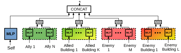
For each agent in SMAC, its observation is first pre-processed, as shown in Fig. 10. The purpose is to make the observation $o_{i}$ of each agent independent of the number of agents in a team by sharing weights between observations of objects of the same types, e.g. allied troops, allied buildings, enemy troops, or enemy buildings.

The strategy to choose actions during exploration (training phase) is $\epsilon-$ greedy. In the experiment, $\epsilon$ is annealing from $0.15$ to $0.05$ during the first $50K$ time steps in the source task and during the first $100K$ time steps in the target task. Each agent does not observe itself ID to learn the index-free policy. The batch size is $32$ episodes. The optimisation is RMSprop with no momentum or weight decay, the learning rate is set as $5\times 10^{-4}$ , and $\alpha=0.99$ . We use the same method as proposed in SMAC paper to evaluate our agents, which is after training for an interval of $10K$ time steps, the learning team will decentralised execute. We then measure the common rewards (for modified prey-predator) or the test win rate (for SMAC).

4.2.2. Role-based Scenarios

To show the ability of our architecture to transfer the individual and mixer networks across team sizes, we construct a set of new scenarios that require strict coordination in SMAC. More specifically, each team has buildings, which serve a similar purpose to the campsites in our enriched prey-predator games in Section 4.1. For example, in a particular setting called 3m_vs_4m_buildings, the learned allied agents control three marines against four enemy marines, and each team has one building to defend. Similarly, in 5m_vs_6m_buildings, the learned allied agents control five marines against six enemy marines; and each team has two buildings to defend (see Fig. 1 in Section 1 for an illustration). The scenario 9m_vs_10m_buildings is more difficult because there are two enemy marines always guarding their buildings, and each team has three buildings.

In our scenarios, the team needs not only to kill the opponent’s troop aggressively but also to defend its buildings and to destroy the enemy buildings. This is because the game will be terminated if all buildings of one team are destroyed. This forces agents to choose the defender or attacker roles when they see fit. At the beginning of an episode, there are enemy marines placed nearby the allied buildings; therefore, defending own buildings is crucial to winning the game.

We compare our algorithm against three major baselines on SMAC: (1) QMIX Rashid et al. 2018: the mixer network captures non-linear and monotonicity properties; (2) ROMA Wang et al. 2020a which learns emergent roles by hyper-network to generate weights of individual agents; (3) DyMA-CL Wang et al. 2020b: transfer individual policy network. We consider the curriculum with the increasing team size and difficulty. The DyMA-CL obtained good results before being transferred to the bigger team size. Our individual and mixer networks are first pre-trained on the team of size 3 (3m_vs_4m_buildings), then transferred to train the team of size 5 (5m_vs_6m_buildings). Finally, it is trained with the team of size 9 (9m_vs_10m_buildings). Figs. 11 and 12 show that our networks trained with LSTRR regulariser can outperform other baselines on the target tasks 5m_vs_6m_buildings and 9m_vs_10m_buildings, respectively. Critically, without the LSTRR, it is impossible to learn to play 9m_vs_10m_buildings at all (Fig. 12).

4.2.3. Improving ROMA

We conducted experiments to test our mixer with ROMA Wang et al. 2020a as individual policies (individual policies include a hyper-network to generate roles) on two benchmark scenarios: (1) 2s3z (classified as a Symmetric and Easy scenario): controlling 2 Stalkers and 3 Zealots to defeat an enemy team which has the same units; (2) MMM2 (classified as an Asymmetric and Hard scenario): controlling $1$ Medivac, $2$ Marauders and $7$ Marines to defeat an enemy team with $1$ Medivac, $3$ Marauders and $8$ Marines. We incorporated our architecture of the mixer into ROMA. Fig. 13 shows that our architecture is more sample efficient than ROMA in both scenarios. The team trained by ROMA has longer episode lengths compared to our method (Fig. 14). To investigate this observation, we compared the test battles of two methods. After $2,000,000$ training time steps, even though teams trained by ROMA and ours could not learn to defeat the enemy, there are significant differences in the agents’ behaviours. We observed the reward hacking phenomenon in the team trained by ROMA. In the middle of an episode, when some agents were killed (the chance for the team to win is small), alive agents retreated to the corner of the map (out of the sight of the enemy). It is reasonable for individual agents to avoid being killed. However, it induces wasteful samples for the training during the end phase of the episodes. All agents in our team, in contrast, engage in the battle and learn the optimal behaviours to win this game.

5. Related Works

Team decomposition

Value decomposition of a team reward in the CTDE paradigm was pioneered by VDN Sunehag et al. 2018 which is a simple linear composition of individual $Q$ -values. Later, QMIX Rashid et al. 2018 improved the composition function by bringing in the global state information and relaxing the linearity into a monotonic linear composition. However, this monotonicity restricts the class of value functions, especially, it could fail to represent the optimal $Q^{*}$ Rashid et al. 2020; Böhmer et al. 2020. To overcome this limitation, QTRAN Son et al. 2019 relaxed the additivity and monotonicity by transforming all value functions to satisfy the Individual-Global-Max (IGM) condition. Alternatively, Qatten Yang et al. 2020a implemented multi-head attention to generate the weights for agents based on their own properties. QPLEX Wang et al. 2021b, on the other hand, used a duelling structure for both joint and individual value functions, which can benefit from off-line RL Levine et al. 2020.

Roles

Another important line of work focuses on training agents to discover behaviours and roles. ROMA Wang et al. 2020a designed a role embedding space and used a hyper-network to model the individual policies conditioned on the role. The authors also introduced regularisers based on diversity and identifiability to encourage the role emergence. RODE Wang et al. 2021a improved upon ROMA on role discovery by decomposing the joint action space into regions associated with different roles, thus learning a role selector and a role policy of lower temporal resolution. In MARL, all agents need to coordinate their actions. Individually exploring the environment could induce a large amount of noisy rewards during training, a non-stationary learning phenomenon Chang et al. 2003. Different from ROMA which only motivates each agent individually to explore optimal behaviour, MAVEN Mahajan et al. 2019 created a framework to explore the space of joint behaviours. While both ROMA and MAVEN applied the technique of conditioning agent behaviours on latent variables, Q-DPP Yang et al. 2020b applied the determinantal point process to improve the coordinated exploration when training an RL team.

Transfer learning in teams

Training good individual policies for a small team size then adjusting these policies for a large team size can be considered as an instance of curriculum learning. Recently, DyMA-CL Wang et al. 2020b proposed a training strategy on top of value based methods to transfer across different team sizes. However, this method does not take into account the learning and transferring roles of agents. Transferring to new team sizes requires learning an index-free policy in which the agent behaviour does not depend on its index in the team. In Le et al. 2017, authors proposed a method to learn roles from a set of experiences. This method distinguishes roles by the trajectories induced by these roles, while our method tries to learn roles based on their effects at different time scales.

Learning multiple horizons has been empirically proved to improve the performance of a single RL agent. The work in Xu et al. 2018 proposed to optimise the discount factor $\gamma$ . The work in Fedus et al. 2019 suggested learning different $Q$ -values for different discount factors as auxiliary tasks. In Romoff et al. 2019, the value function is broken down into different components based on smaller discount factors. Recently, it has been suggested in Amit et al. 2020 the use of reduced discount factors to estimate the value function in temporal difference learning, especially when the amount of data is limited. However, these works only focus on using different discount factors to facilitate training a single reinforcement learning agent; we investigate the use of different discount factors in multi-agent learning, realising under the concept of roles.

6. Conclusion

We have introduced a new multi-agent reinforcement learning framework to help scale an important paradigm known as centralised training decentralised execution (CTDE). We redesigned the mixing network in the popular QMIX framework to enable (i) learning with arbitrary team sizes; (ii) assigning credits to roles, each of which evaluates and attributes contributions from individual agents; and (iii) curriculum learning process that starts from smaller teams and progresses to large teams. We also contributed two suites of MARL experiments to evaluate strongly cooperative CTDE tasks that demand the notion of roles dynamically played by the agents. One suite enriches the Prey-Predator games to include more types, roles and skills. The other suite of experiments extends the StarCraft II Micro-Management tasks. We demonstrated that the proposed framework leads to faster convergence and the emergence of roles and can succeed in certain large team settings.

References

(1)
Amit et al. (2020) Ron Amit, Ron Meir, and Kamil Ciosek. 2020. Discount factor as a regularizer in reinforcement learning. In International conference on machine learning. PMLR, 269–278.
Biddle (2013) Bruce J Biddle. 2013. Role theory: Expectations, identities, and behaviors. Academic Press.
Böhmer et al. (2020) Wendelin Böhmer, Vitaly Kurin, and Shimon Whiteson. 2020. Deep coordination graphs. In International Conference on Machine Learning. PMLR, 980–991.
Buşoniu et al. (2010) Lucian Buşoniu, Robert Babuška, and Bart De Schutter. 2010. Multi-agent reinforcement learning: An overview. Innovations in multi-agent systems and applications-1 (2010), 183–221.
Chang et al. (2003) Yu-Han Chang, Tracey Ho, and Leslie Kaelbling. 2003. All learning is local: Multi-agent learning in global reward games. Advances in neural information processing systems 16 (2003), 807–814.
Chung et al. (2014) Junyoung Chung, Caglar Gulcehre, KyungHyun Cho, and Yoshua Bengio. 2014. Empirical evaluation of gated recurrent neural networks on sequence modeling. arXiv preprint arXiv:1412.3555 (2014).
Elman (1993) Jeffrey L Elman. 1993. Learning and development in neural networks: The importance of starting small. Cognition 48, 1 (1993), 71–99.
Fedus et al. (2019) William Fedus, Carles Gelada, Yoshua Bengio, Marc G Bellemare, and Hugo Larochelle. 2019. Hyperbolic discounting and learning over multiple horizons. arXiv preprint arXiv:1902.06865 (2019).
Foerster et al. (2018) Jakob Foerster, Gregory Farquhar, Triantafyllos Afouras, Nantas Nardelli, and Shimon Whiteson. 2018. Counterfactual multi-agent policy gradients. In Proceedings of the AAAI Conference on Artificial Intelligence, Vol. 32.
Gupta et al. (2017) Jayesh K Gupta, Maxim Egorov, and Mykel Kochenderfer. 2017. Cooperative multi-agent control using deep reinforcement learning. In International Conference on Autonomous Agents and Multiagent Systems. Springer, 66–83.
Ha et al. (2017) David Ha, Andrew Dai, and Quoc V Le. 2017. HyperNetworks. ICLR (2017).
Hinton and Plaut (1987) Geoffrey E Hinton and David C Plaut. 1987. Using fast weights to deblur old memories. In Proceedings of the ninth annual conference of the Cognitive Science Society. 177–186.
Kraemer and Banerjee (2016) Landon Kraemer and Bikramjit Banerjee. 2016. Multi-agent reinforcement learning as a rehearsal for decentralized planning. Neurocomputing 190 (2016), 82–94.
Le et al. (2017) Hoang M Le, Yisong Yue, Peter Carr, and Patrick Lucey. 2017. Coordinated multi-agent imitation learning. arXiv preprint arXiv:1703.03121 (2017).
Levine et al. (2020) Sergey Levine, Aviral Kumar, George Tucker, and Justin Fu. 2020. Offline reinforcement learning: Tutorial, review, and perspectives on open problems. arXiv preprint arXiv:2005.01643 (2020).
Lowe et al. (2017) Ryan Lowe, Yi I Wu, Aviv Tamar, Jean Harb, OpenAI Pieter Abbeel, and Igor Mordatch. 2017. Multi-agent actor-critic for mixed cooperative-competitive environments. In Advances in neural information processing systems. 6379–6390.
Mahajan et al. (2019) Anuj Mahajan, Tabish Rashid, Mikayel Samvelyan, and Shimon Whiteson. 2019. Maven: Multi-agent variational exploration. In Advances in Neural Information Processing Systems. 7613–7624.
Matignon et al. (2012) Laetitia Matignon, Guillaume J Laurent, and Nadine Le Fort-Piat. 2012. Independent reinforcement learners in cooperative markov games: a survey regarding coordination problems. The Knowledge Engineering Review 27, 1 (2012), 1–31.
Narvekar et al. (2020) Sanmit Narvekar, Bei Peng, Matteo Leonetti, Jivko Sinapov, Matthew E. Taylor, and Peter Stone. 2020. Curriculum Learning for Reinforcement Learning Domains: A Framework and Survey. J. Mach. Learn. Res. 21 (2020), 181:1–181:50.
Narvekar and Stone (2019) Sanmit Narvekar and Peter Stone. 2019. Learning Curriculum Policies for Reinforcement Learning. In Proceedings of the 18th International Conference on Autonomous Agents and MultiAgent Systems. 25–33.
Oliehoek and Amato (2016) Frans A. Oliehoek and Christopher Amato. 2016. A Concise Introduction to Decentralized POMDPs. Springer.
Oliehoek et al. (2008) Frans A Oliehoek, Matthijs TJ Spaan, and Nikos Vlassis. 2008. Optimal and approximate Q-value functions for decentralized POMDPs. Journal of Artificial Intelligence Research 32 (2008), 289–353.
Omidshafiei et al. (2017) Shayegan Omidshafiei, Jason Pazis, Christopher Amato, Jonathan P How, and John Vian. 2017. Deep decentralized multi-task multi-agent reinforcement learning under partial observability. In International Conference on Machine Learning. PMLR, 2681–2690.
Rashid et al. (2020) Tabish Rashid, Gregory Farquhar, Bei Peng, and Shimon Whiteson. 2020. Weighted QMIX: Expanding Monotonic Value Function Factorisation for Deep Multi-Agent Reinforcement Learning. In Advances in Neural Information Processing Systems 33: Annual Conference on Neural Information Processing Systems 2020, NeurIPS 2020, virtual.
Rashid et al. (2018) Tabish Rashid, Mikayel Samvelyan, Christian Schröder de Witt, Gregory Farquhar, Jakob N. Foerster, and Shimon Whiteson. 2018. QMIX: Monotonic Value Function Factorisation for Deep Multi-Agent Reinforcement Learning. In Proceedings of the 35th International Conference on Machine Learning, ICML 2018, Stockholmsmässan, Stockholm, Sweden. PMLR, 4292–4301.
Romoff et al. (2019) Joshua Romoff, Peter Henderson, Ahmed Touati, Yann Ollivier, Emma Brunskill, and Joelle Pineau. 2019. Separating value functions across time-scales. CoRR abs/1902.01883 (2019). http://arxiv.org/abs/1902.01883
Samvelyan et al. (2019a) Mikayel Samvelyan, Tabish Rashid, Christian Schroeder de Witt, Gregory Farquhar, Nantas Nardelli, Tim G. J. Rudner, Chia-Man Hung, Philiph H. S. Torr, Jakob Foerster, and Shimon Whiteson. 2019a. The StarCraft Multi-Agent Challenge. CoRR abs/1902.04043 (2019).
Samvelyan et al. (2019b) Mikayel Samvelyan, Tabish Rashid, Christian Schroeder de Witt, Gregory Farquhar, Nantas Nardelli, Tim GJ Rudner, Chia-Man Hung, Philip HS Torr, Jakob Foerster, and Shimon Whiteson. 2019b. The StarCraft Multi-Agent Challenge. In Proceedings of the 18th International Conference on Autonomous Agents and MultiAgent Systems. 2186–2188.
Schmidhuber (1992) Jürgen Schmidhuber. 1992. Learning to control fast-weight memories: An alternative to dynamic recurrent networks. Neural Computation 4, 1 (1992), 131–139.
Son et al. (2019) Kyunghwan Son, Daewoo Kim, Wan Ju Kang, David Earl Hostallero, and Yung Yi. 2019. Qtran: Learning to factorize with transformation for cooperative multi-agent reinforcement learning. arXiv preprint arXiv:1905.05408 (2019).
Sunehag et al. (2018) Peter Sunehag, Guy Lever, Audrunas Gruslys, Wojciech Marian Czarnecki, Vinícius Flores Zambaldi, Max Jaderberg, Marc Lanctot, Nicolas Sonnerat, Joel Z Leibo, Karl Tuyls, et al. 2018. Value-Decomposition Networks For Cooperative Multi-Agent Learning Based On Team Reward. In AAMAS. 2085–2087.
Tan (1993) Ming Tan. 1993. Multi-agent reinforcement learning: Independent vs. cooperative agents. In Proceedings of the tenth international conference on machine learning. 330–337.
Wang et al. (2021b) Jianhao Wang, Zhizhou Ren, Terry Liu, Yang Yu, and Chongjie Zhang. 2021b. QPLEX: Duplex Dueling Multi-Agent Q-Learning. In 9th International Conference on Learning Representations, ICLR 2021, Virtual Event, Austria.
Wang et al. (2020a) Tonghan Wang, Heng Dong, Victor R. Lesser, and Chongjie Zhang. 2020a. ROMA: Multi-Agent Reinforcement Learning with Emergent Roles. ICML abs/2003.08039 (2020). https://arxiv.org/abs/2003.08039
Wang et al. (2021a) Tonghan Wang, Tarun Gupta, Anuj Mahajan, Bei Peng, Shimon Whiteson, and Chongjie Zhang. 2021a. RODE: Learning Roles to Decompose Multi-Agent Tasks. ICLR (2021).
Wang et al. (2020b) Weixun Wang, Tianpei Yang, Yong Liu, Jianye Hao, Xiaotian Hao, Yujing Hu, Yingfeng Chen, Changjie Fan, and Yang Gao. 2020b. From Few to More: Large-Scale Dynamic Multiagent Curriculum Learning. In The Thirty-Fourth AAAI Conference on Artificial Intelligence, AAAI 2020. 7293–7300. https://aaai.org/ojs/index.php/AAAI/article/view/6221
Xu et al. (2018) Zhongwen Xu, Hado P van Hasselt, and David Silver. 2018. Meta-gradient reinforcement learning. Advances in neural information processing systems 31 (2018), 2396–2407.
Yang et al. (2020a) Yaodong Yang, Jianye Hao, Ben Liao, Kun Shao, Guangyong Chen, Wulong Liu, and Hongyao Tang. 2020a. Qatten: A General Framework for Cooperative Multiagent Reinforcement Learning. arXiv preprint arXiv:2002.03939 (2020).
Yang et al. (2020b) Yaodong Yang, Ying Wen, Lihuan Chen, Jun Wang, Kun Shao, David Mguni, and Weinan Zhang. 2020b. Multi-Agent Determinantal Q-Learning. arXiv preprint arXiv:2006.01482 (2020).
Zhang et al. (2021) Kaiqing Zhang, Zhuoran Yang, and Tamer Başar. 2021. Multi-agent reinforcement learning: A selective overview of theories and algorithms. Handbook of Reinforcement Learning and Control (2021), 321–384.