跳到论文正文
W Papers独立论文阅读器 arXiv:2204.12866 论文正文 计算阅读时间 · 0%
引用这篇论文根据当前论文元数据生成,正式投稿前建议核对。


License: CC BY 4.0
arXiv:2204.12866v1 [math.AP] 27 Apr 2022

Universidade Federal da Paraíba

Programa de Pós-Graduação em Matemática

Doutorado em Matemática

Fractional one-sided measure theoretic second-order elliptic operators and applications to stochastic partial differential equations

por

Kelvin Jhonson Ribeiro de Sousa Almeida Silva

João Pessoa - PB

Fevereiro/2022

Fractional one-sided measure theoretic second-order elliptic operators and applications to stochastic partial differential equations

por

Kelvin Jhonson Ribeiro de Sousa Almeida Silva†† † Este trabalho contou com apoio financeiro da CAPES.

sob orientação do

Prof. Dr. Alexandre de Bustamante Simas

Tese apresentada ao Corpo Docente do Programa de Pós-Graduação em Matemática - UFPB, como requisito parcial para obtenção do título de Doutor em Matemática.

João Pessoa - PB

Fevereiro/2022

Abstract

In this work we introduce and study fractional measure theoretic elliptic operators on the torus and a new stochastic process named W-Brownian motion. We establish some regularity and spectral results related to the operators cited above, more precisely, we were able to provide sharp bounds for the growth rate of eigenvalues to an associated eigenvalue problem. Moreover, we show how the Cameron-Martin space associated to the W-Brownian motion relates to Sobolev spaces connected with the elliptic operators mentioned above. Finally applications of the theory developed on stochastic partial differential equations are given.

Keywords: Fractional Sobolev Spaces; Brownian Motion; Elliptic Operators.

Resumo

Neste trabalho apresentamos e estudamos os operadores elípticos unilaterais fracionários no sentido teorético da medida sobre o toro e um novo processo estocástico denominado movimento W-Browniano. Estabelecemos alguns resultados de regularidade e espectrais relacionados aos operadores citados acima, mais precisamente, fomos capazes de fornecer limites nítidos para a taxa de crescimento de autovalores para um problema de autovalor associado. Além disso, mostramos como o espaço de Cameron-Martin associado ao movimento W-Browniano se relaciona com espaços Sobolev naturalmente associado aos operadores elípticos mencionados anteriormente. Finalmente, fornecemos algumas aplicações da teoria deselvolvida em equações diferenciais parciais estocásticas.

Keywords: Espaços de Sobolev Fracionários; Movimento Browniano; Operadores Elípticos.

Agradecimentos

Agradeço primeiramente a DEUS por ter abençoado meu caminho e ter permitido que eu chegasse até aqui, garantindo a minha saúde e paz fronte as eventuais adversidades que nem mesmo pude perceber que estavam presentes.

Ao professor Alexandre de Bustamente Simas por toda a paciência e apoio, pelos valorosos conselhos de vida e também por todo conhecimento matemático que ele compartilhou comigo ao longo desta etapa de minha vida. Sua participação foi de fundamental importância para a realização deste sonho.

Aos meus famíliaares por todo apoio moral ao longo deste período do Doutorado e também por entenderem os evetuais momentos em que precisei estar um pouco ausente, em especial a minha querida mãe Ivanda Ribeiro de Sousa.

A minha amada Mirian dos Santos Mendes por ter acreditado no meu potencial, por todo o companheirismo e por estar do meu lado em um dos momentos mais difíceis que tive ao longo do Doutorado. Meus agradecimentos também a sua família por todo o apoio.

A todos os amigos, colegas e professores que tive a oportunidade de conhecer e estudar ao longo de todo meu período acadêmico, o acolhimento de vocês foi essencial. Agradeço a cada um destes que, entre um copo e outro de café, puderam me ensinar um pouco mais sobre a vida e me tornaram uma pessoa melhor.

A CAPES, pelo apoio financeiro.

A todos que de alguma forma me ajudaram.

“Que ninguém se engane, só se consegue a simplicidade através de muito trabalho.”

Clarice Lispector

Dedicatória

A todos os meus professores, e colegas do meio acadêmico.

Introduction

A class of second order differential operators dd​V​dd​x\frac{d}{dV}\frac{d}{dx} introduced by W. Feller in [14] gave rise to research in many different mathematical fields, for instance in the field of stochastic differential equations, real analysis, fractal geometry, etc. We can cite [16, 15, 12] and [29] to name a few. On the other hand, [25], along with some other works from the same authors, have focused their attention in an interesting way to define a consistent local definition of the derivative in the sense of Stieltjes in such a way that some useful results in analysis can be re-obtained as a consequence of local definition of such Stieltjes derivatives. On another direction, Franco and Landim [15] studied the formal adjoint of Feller’s original operator, which is given by dd​x​dd​W\frac{d}{dx}\frac{d}{dW}, that is, in a way (since [16] requires the measure induced by WW to be nonatomic, whereas in [15] there is no such a restriction), a particular case of the operator dd​V​dd​W\frac{d}{dV}\frac{d}{dW} introduced by Uta in [16]. However, unlike Uta [16], Franco and Landim [15] started with a local operator that was defined in a manner that it depends on a type of Stieltjes derivative of càdlàg functions. The link between the operators in [16] and [15] is very interesting and some intriguing questions emerge from the different approaches adopted to the study these second-order operators.

On the second chapter of this thesis we provide a general operator that can connect, in some sense, all of the operators above. We begin by considering the approach of [15] to generalize the formal operator dd​V​dd​W\frac{d}{dV}\frac{d}{dW}. This operator, which comes from a local definition, agrees with the “global” operator introduced in [16] in the case the measures induced by VV and WW are atomless. Note that we do not require such a restriction. Further, we work with a generalization of the one-sided derivatives, which can be understood as a one-sided derivative in the Stieltjes sense. More precisely, we fix two increasing functions W,V:ℝ→ℝW,V:\mathbb{R}\to\mathbb{R} where WW is a càdlàd (a right-continuous function with left limits) function and VV is a càglàd (a left-continuous function with right limits) function that satisfy some periodic conditions to properly define finite Borel measures d​WdW and d​VdV on 𝕋=ℝ/ℤ\mathbb{T}=\mathbb{R}/\mathbb{Z}. With the assumptions on VV and WW in mind, we say that f:𝕋→ℝf:\mathbb{T}\to\mathbb{R} is WW-left differentiable or VV-right differentiable, respectively, according to the existence of the limits

DW−​f​(x):=limh→0−f⁡(x+h)−f⁡(x)W⁡(x+h)−W⁡(x)D^{-}_{W}f(x):=\lim_{h\to 0^{-}}\frac{f(x+h)-f(x)}{W(x+h)-W(x)}

or

DV+​f​(x):=limh→0+f⁡(x+h)−f⁡(x)V⁡(x+h)−V⁡(x)D^{+}_{V}f(x):=\lim_{h\to 0^{+}}\frac{f(x+h)-f(x)}{V(x+h)-V(x)}

for all x∈𝕋.x\in\mathbb{T}. By using these notions of generalized one-sided derivatives, we introduce the domain 𝔇W,V\mathfrak{D}_{W,V} of the new symmetric and non-positive second order operator

DV+​(DW−):𝔇W,V⊂LV2​(𝕋)→LV2​(𝕋).D^{+}_{V}(D^{-}_{W}):\mathfrak{D}_{W,V}\subset L^{2}_{V}(\mathbb{T})\to L^{2}_{V}(\mathbb{T}).

At this point is very important pay attention on the subscript “W,V”, whenever we change the order of the functions, it means that we are considering the “dual” scenario, in which we reverse the operations between VV and WW. Furthermore, the operator DV+​(DW−)D^{+}_{V}(D^{-}_{W}) satisfies all the required hypothesis to ensure the existence of the Friedrichs extension. Let, then, (I−ΔW,V):𝒟W,V⊂LV2​(𝕋)→LV2​(𝕋)\left(I-\Delta_{W,V}\right):\mathcal{D}_{W,V}\subset L^{2}_{V}(\mathbb{T})\to L^{2}_{V}(\mathbb{T}) be the Friedrichs extension of the operator I−DV+​DW−I-D_{V}^{+}D_{W}^{-}, and let the associated energetic space be given by HW,V​(𝕋)H_{W,V}(\mathbb{T}). Moreover, define the formal second order operator

ΔW,V:=I−(I−ΔW,V):𝒟W,V⊂LV2​(𝕋)→LV2​(𝕋)\Delta_{W,V}:=I-(I-\Delta_{W,V}):\mathcal{D}_{W,V}\subset L^{2}_{V}(\mathbb{T})\to L^{2}_{V}(\mathbb{T})

that can be understood as the model for the measure theoretic Laplacian dd​V​dd​W\frac{d}{dV}\frac{d}{dW} introduced on the torus. One notable result we were able to obtain is refers to the regularity of the eigenvectors of the problem

{−ΔW,Vϕ=λϕ,λ∈ℝ∖{0};u∈𝒟W,V​(𝕋).\begin{cases}-\Delta_{W,V}\phi=\lambda\phi,\,\lambda\in\mathbb{R}\setminus\{0\};\\ u\in\mathcal{D}_{W,V}(\mathbb{T}).\end{cases}

We proved that each solution ϕ\phi of the above problem belongs to the space CW,V∞​(𝕋)C^{\infty}_{W,V}(\mathbb{T}), that is the space of càdlàg functions f:𝕋→ℝf:\mathbb{T}\to\mathbb{R} such that DW−​fD^{-}_{W}f exists and is a zero-mean càglàd function, DV+​(DW−​f)D^{+}_{V}(D^{-}_{W}f) exists and is zero-mean càdlàg function, DW−​[DV+​(DW−​f)]D^{-}_{W}[D^{+}_{V}(D^{-}_{W}f)] exists and is a zero-mean càglàd function, and so on. The space CW,V∞​(𝕋)C^{\infty}_{W,V}(\mathbb{T}) will work as a new space of test functions to define the notion of WW-left weak derivative that will allow us to characterize the space HW.V​(𝕋)H_{W.V}(\mathbb{T}) as a WW-VV-Sobolev space. Furthermore, we can characterize the space HW,V​(𝕋)H_{W,V}(\mathbb{T}) in terms of the Fourier coefficients of the functions. More precisely, we prove that

HW,V(𝕋)={f∈LV2(𝕋);f=α0+∑i=1∞αiνi;∑i=1∞λiαi2<∞},H_{W,V}(\mathbb{T})=\left\{f\in L^{2}_{V}(\mathbb{T});f=\alpha_{0}+\sum_{i=1}^{\infty}\alpha_{i}\nu_{i};\sum_{i=1}^{\infty}\lambda_{i}\alpha_{i}^{2}<\infty\right\},

where {λi}i≥1\{\lambda_{i}\}_{i\geq 1} are the eigenvalues of the operator −ΔW,V-\Delta_{W,V} which exist due to the compact immersion of HW,V​(𝕋)H_{W,V}(\mathbb{T}) into LV2​(𝕋)L^{2}_{V}(\mathbb{T}), which we proved in Theorem 1.2.5.\ref{compactemb}. After some applications on partial differential equations, we introduce, on the subsection 2.7 a new generalization of the Brownian motion, and called WW-Brownian motion, denoted by BWB_{W}, which possess the following properties:

  1. 1.

    The finite-dimensional distributions of BWB_{W} are Gaussian;

  2. 2.

    The sample paths of BWB_{W} are càdlàg and may have jumps.

Satisfy both conditions at the same time are uncommon features in the literature in the range of generalizations of the Brownian motion. Moreover, we establish a very deep and intimate connection between the WW-Brownian motion when we obtain the Cameron-Martin space of BWB_{W} as the space HW,V,𝒟​(𝕋)={f∈HW,V​(𝕋):f⁡(0)=0}H_{W,V,\mathcal{D}}(\mathbb{T})=\{f\in H_{W,V}(\mathbb{T}):f(0)=0\}. This shows that the Cameron-Martin space of BWB_{W} is, actually, our WW-VV-Sobolev space with a Dirichlet condition. This, in turn, shows that the WW-Brownian motion can be obtained as the process whose distribution in LV2​(𝕋)L^{2}_{V}(\mathbb{T}) is the unique Gaussian measure associated to the Cameron-Martin space HW,V,𝒟​(𝕋)H_{W,V,\mathcal{D}}(\mathbb{T}). Finally, some applications to stochastic partial differential equations are presented.

In Chapter 3, we provide sufficient conditions for a functions on CW,V∞​(𝕋)C^{\infty}_{W,V}(\mathbb{T}) to be represented as an analogue of MacLaurin series expansion. This representation can be seen as the WW-VV-version of analytical functions. Thus, we provide sufficient conditions for a function to be analytical in some sense. More precisely, if we define F1​(x)=W​(x)F_{1}(x)=W(x) and recursively define

Fn​(x,s)={∫[0,s)[Fn−1​(x,x)−Fn−1​(x,ξ)]​dV​(ξ),n even;∫(0,s][Fn−1​(x,x)−Fn−1​(x,ξ)]​dW​(ξ),n odd,F_{n}(x,s)=\begin{cases}\displaystyle\int_{[0,s)}\left[F_{n-1}(x,x)-F_{n-1}(x,\xi)\right]dV(\xi),\;\mbox{n even};\\ \displaystyle\int_{(0,s]}\left[F_{n-1}(x,x)-F_{n-1}(x,\xi)\right]dW(\xi),\;\mbox{n odd},\end{cases}

then the sequence {Fk​(x,x)}k≥1\{F_{k}(x,x)\}_{k\geq 1} plays the role of the polynomial terms xnn!\dfrac{x^{n}}{n!} in the classical MacLaurin expansion for W⁡(x)=V⁡(x)=xW(x)=V(x)=x. We provide suitable assumptions on the decay of the sequence given by the one-sided derivatives of ff at 00 denoted by DW,Vn​f​(0)D^{n}_{W,V}f(0), under which, we can obtain the uniform convergence of ∑k=1kDW,V(n)​f​(0)​Fn​(x,x)\sum_{k=1}^{k}D^{(n)}_{W,V}f(0)F_{n}(x,x) on 𝕋\mathbb{T}. We also found the compatibility conditions to ensure that the series will be well defined on 𝕋\mathbb{T}. Moreover, all these results allowed us to determine a representation of the eigenvectors νi\nu_{i} of −ΔW,V-\Delta_{W,V} in terms of the measure theoretic trigonometric functions SW,V​(α,x)S_{W,V}(\alpha,x), CW,V​(α,x)C_{W,V}(\alpha,x), SV,W​(α,x)S_{V,W}(\alpha,x) and CV,W​(α,x)C_{V,W}(\alpha,x) that are generalizations of the classical trigonometric functions cos⁡(α​x)\cos(\alpha x) and sin⁡(α​x)\sin(\alpha x). In this chapter we also introduce the fractional order WW-VV-Sobolev spaces, which as defined in terms of their Fourier coefficients:

𝒟(I−ΔW,V)s/2:=HW,Vs(𝕋)={f∈LV2(𝕋);f=α0+∑i=1∞αiνi;∑i=1∞λisαi2<∞},\mathscr{D}(I-\Delta_{W,V})^{s/2}:=H^{s}_{W,V}(\mathbb{T})=\left\{f\in L^{2}_{V}(\mathbb{T});f=\alpha_{0}+\sum_{i=1}^{\infty}\alpha_{i}\nu_{i};\sum_{i=1}^{\infty}\lambda_{i}^{s}\alpha_{i}^{2}<\infty\right\},

for s∈ℝs\in\mathbb{R}. By using measure trigonometrical characterization of the eigenvectors of −ΔW,V-\Delta_{W,V} we were able to prove, by using the theory of entire functions, the existence of ρ∈(0,1/2]\rho\in(0,1/2] such that

∑i=1∞1λis\sum_{i=1}^{\infty}\frac{1}{\lambda_{i}^{s}}

forall s>ρs>\rho, or equivalently, that the operator (I−ΔW,V)s/2(I-\Delta_{W,V})^{s/2} is trace class for s>ρ.s>\rho. We then provide a generalization of the results for dimensions dd. That is, we introduced the generalized Laplacian on the dd-dimensional torus 𝕋d\mathbb{T}^{d} by taking tensor products of the eigenvectors of ΔW,V\Delta_{W,V}. We, then, provide dd-dimensional counterparts to several results obtained for dimensions 1. The most remarkable being that for s>d/2s>d/2 the operator (I−ΔW,V)s/2(I-\Delta_{W,V})^{s/2} is trace class, recovering the same lower bound for the Laplacian on 𝕋d\mathbb{T}^{d}. Finally, Chapter 3 ends with some applications on second order stochastic differential equations.

The thesis is concluded with a final discussion on some interesting open problems related to this theory.

Chapter 1 One-sided measure theoretic Laplacian and applications

Recently some works have studied classes of generalized differential operators based on the concept of derivative DW:=dd​WD_{W}:=\frac{d}{dW} with respect to an increasing function W:ℝ→ℝW:\mathbb{R}\to\mathbb{R} which is right-continuous (or left-continuous). See, for instance, [11, 25, 29, 1, 16] and [15].

Note that the second-order differencial operator dd​x​(dd​W)\frac{d}{dx}\left(\frac{d}{dW}\right) introduced in [11] have one of its derivatives with respect to WW which may have jumps, and surprisingly these jumps of WW can be dense in ℝ.\mathbb{R}. This last observations ensures that regular functions with respect to such derivatives will, most likely, have discontinuity points. Typically, we will look for functions that are right-continuous and have left limits. On the other hand, it is noteworthy that the differential operator dd​W​(dd​x)​f\frac{d}{dW}\left(\frac{d}{dx}\right)f introduced by Feller in his seminal paper [14] requires an initial space contained on the space of continuous functions, this is due to the requirement of the existence of the first derivative in the strong sense (and being derivatives from both sides, not only lateral derivatives). One should note that all the aforementioned operators generalize the usual laplacian operator dd​x​(dd​x)\frac{d}{dx}\left(\frac{d}{dx}\right), which is the case when W⁡(x)=xW(x)=x.

In [29, 30] they introduced the WW-Sobolev spaces and obtained some elliptic regularity. They showed that the generalized derivative can be seen in the Sobolev perspective. However, as will also be discussed in Section 1.3, the usage of two-sided derivatives, meaning that the standard limit is taken in the definition of the derivative, instead of lateral limits, had a serious impact on the regularity study of such operators. Indeed, the space of regular functions on the WW-Sobolev spaces, that arise from eigenvectors of the operators, which should be considered smooth, cannot be evaluated pointwisely. This shows a need for an adaptation of this theory, in such a way that we create a new type of WW-Sobolev space (which here will be more general, and we will call WW-VV-Sobolev spaces), with a nice regularity theory that allows for pointwise evaluations, but also agrees with the WW-Sobolev spaces in [29] and also with the standard Sobolev spaces, see Remark 1.2.4.

The first goal of this paper is to consider a general one-sided second order differential operator in such a way that it generalizes at the same time both differential operators we mentioned above, namely dd​W​(dd​x)\frac{d}{dW}\left(\frac{d}{dx}\right) and dd​x​(dd​W)\frac{d}{dx}\left(\frac{d}{dW}\right). Indeed, we explain on Remark 1.1.5 how we can re-obtain these differential operator by just imposing regularity conditions on the range of those operators. On the second moment, given the generalized Laplacian ΔW,V\Delta_{W,V}, introduced in Definition 1.2.8, we will introduce the natural space CW,V∞​(𝕋)C^{\infty}_{W,V}(\mathbb{T}) where all eigenfunctions of the problem

{−ΔW,Vϕ=λϕ,λ∈ℝ∖{0};u∈𝒟W,V​(𝕋),\begin{cases}-\Delta_{W,V}\phi=\lambda\phi,\,\lambda\in\mathbb{R}\setminus\{0\};\\ u\in\mathcal{D}_{W,V}(\mathbb{T}),\end{cases} (1.1)

belong, and following the ideas of [29] we introduce and new (W,V)(W,V)-Sobolev space HW,V​(𝕋)H_{W,V}(\mathbb{T}) and characterize this last space from other different perspectives. The insight to consider the space CW,V∞​(𝕋)C^{\infty}_{W,V}(\mathbb{T}) is due to the regularity problem associated to the eigenvectors determined by the operator ℒW\mathcal{L}_{W} studied in [15] which we expected that each of them (almost surely) inherit the "interacted" regularity of the initial space 𝔇W\mathfrak{D}_{W}. We then apply the theory developed to analyze some existence results related to the one-sided second order elliptic equations.

Finally, to conclude the paper, we introduce the WW-Brownian motion, which at first do not appear to be connected to these WW-VV-Sobolev spaces. However, the connection between the WW-Brownian motion and the WW-VV-Sobolev spaces is very deep. Indeed, we show that the WW-VV-Sobolev space is the Cameron-Martin space of the distribution of the WW-Brownian motion. As it is well-known, the Cameron-Martin space, in a sense, uniquely determines the Gaussian measure. So, the Gaussian measure associated to the WW-VV-Sobolev space is the law of the WW-Brownian motion.

1.1 The one-sided differential operator

In this section we begin by introducing our differential operator in the strong sense, acting locally on functions. Then, we use it to define a strong second-order differential operator that extends the second derivative. After that, we show that we can extend this second-order differential operator to a self-adjoint operator which extends the Laplacian. This operator turns out to have a compact resolvent.

Let us introduce some notation. First, we say that a function is càdlàg (from french, “continue à droite, limite à gauche”) if the function is right-continuous and has limits from the left. Similarly, we say that a function is càglàd, if the function is left-continuous and has limits from the right.

Let W,V:ℝ→ℝW,V:\mathbb{R}\to\mathbb{R} be increasing functions that are, respectively, càdlàg and càglàd. Further, we assume that they are periodic in the sense that

∀x∈ℝ,{W⁡(x+1)−W⁡(x)=W⁡(1)−W⁡(0);V⁡(x+1)−V⁡(x)=V⁡(1)−V⁡(0),\forall x\in\mathbb{R},\quad\begin{cases}W(x+1)-W(x)=W(1)-W(0);\\ V(x+1)-V(x)=V(1)-V(0),\end{cases} (1.2)

Without loss of generality we will assume that both WW and VV are continuous at zero, that is, W⁡(0)=0W(0)=0 and V⁡(0)=0V(0)=0. Indeed, since they are increasing, they can only have countably many discontinuities points, so if they are not continuous at zero, we can simply choose another point in which both of them are continuous and translate the functions to make them continuous at zero. Note that WW and VV, thus, induce finite measures on 𝕋=ℝ/ℤ\mathbb{T}=\mathbb{R}/\mathbb{Z}. We will now provide definitions of the one-sided differential operators. We begin by provinding their definitions in a strong sense, meaning that we see them as pointwise lateral limits, thus they act locally on functions.

Note that in the above definition we allow the measures induced by WW and VV to have atoms. This is a weaker assumption than some of the common assumptions found in literature, e.g., [16], [1], among others.

We will denote the L2L^{2} space with the measure induced by VV by LV2​(𝕋)L^{2}_{V}(\mathbb{T}) and its norm (resp. inner product) by ∥⋅∥V\|\cdot\|_{V} (resp. ⟨⋅,⋅⟩V\langle\cdot,\cdot\rangle_{V}). Similarly, we will denote the L2L^{2} space with the measure induced by WW by LW2​(𝕋)L^{2}_{W}(\mathbb{T}) and its norm (resp. inner product) by ∥⋅∥W\|\cdot\|_{W} (resp. ⟨⋅,⋅⟩W\langle\cdot,\cdot\rangle_{W}).

Definition 1.1.1.

We say that a function f:𝕋→ℝf:\mathbb{T}\to\mathbb{R} is WW-left differentiable if

DW−​f​(x):=limh→0−f⁡(x+h)−f⁡(x)W⁡(x+h)−W⁡(x)D^{-}_{W}f(x):=\lim_{h\to 0^{-}}\frac{f(x+h)-f(x)}{W(x+h)-W(x)}

exists for all x∈𝕋x\in\mathbb{T}. Similarly, we say that a function g:𝕋→ℝg:\mathbb{T}\to\mathbb{R} is VV-right differentiable if the limit

DV+​g​(x):=limh→0+g⁡(x+h)−g⁡(x)V⁡(x+h)−V⁡(x)D^{+}_{V}g(x):=\lim_{h\to 0^{+}}\frac{g(x+h)-g(x)}{V(x+h)-V(x)}

exists for all x∈𝕋x\in\mathbb{T}.

The above definition of generalized lateral derivatives, besides having its natual appeal as a straightforward generalization of Newton’s quotient, is also naturally obtained as the derivative operator when differentiating point processes with respect to a Borel measure. See, for instance, [17]. It is also noteworthy that this definition is very general and will allow a proper regularity study. For instance, [29, 30, 31, 15] considered a similar operator when V⁡(x)=xV(x)=x, and when the derivative is not a lateral one. The drawback in their approach is that one cannot obtain a pointwise regularity theory. For instance, the eigenvectors of the differential operators considered in [29, 30, 31, 15] can only be viewed in the L2L^{2}-sense, which was the reason the authors in [31] needed to create an auxiliary space for test functions and also obtain several results exclusively to deal with the lack of regularity. We will discuss more about that in Section 1.3.

A natural question is related to Definition 1.1.1 is if we have a suitable class of functions that are differentiable in this sense. More specifically, we are interested in the functions that are twice differentiable, meaning that they are differentiable with respect to DW−D_{W}^{-}, and that the resulting function is further differentiable with respect to DV+D_{V}^{+}. Let us study such a class.

Definition 1.1.2.

We will denote by 𝔇W,V​(𝕋)\mathfrak{D}_{W,V}(\mathbb{T}) the set of càdlàg functions ff such that:

  • •

    ff is WW-left differentiable.

  • •

    DW−​fD^{-}_{W}f is a càglàd function that is VV-right differentiable.

  • •

    DV+​(DW−​f)D^{+}_{V}(D^{-}_{W}f) is a càdlàg function.

Let us prove an auxiliary lemma that will help us characterization the functions in 𝔇W,V​(𝕋)\mathfrak{D}_{W,V}(\mathbb{T}).

Lemma 1.1.3.

If f:𝕋→ℝf:\mathbb{T}\to\mathbb{R} is càglàd and DV+​f≡0D^{+}_{V}f\equiv 0, then f≡C,f\equiv C, where CC is a constant. Similarly, if g:𝕋→ℝg:\mathbb{T}\to\mathbb{R} is càdlàg and DW−​g≡0D^{-}_{W}g\equiv 0, then g≡Cg\equiv C, where CC is a constant.

Proof.

We will only prove the statement for ff, since the other is entirely analogous. To this end, let us assume, by contradiction, that f⁡(a)≠f⁡(b)f(a)\neq f(b), for some a,ba,b, with a<ba<b. Let

ϵ:=|f⁡(b)−f⁡(a)|2​[V​(b)−V​(a)],\epsilon:=\frac{|f(b)-f(a)|}{2\left[V(b)-V(a)\right]},

and c=inf{x;x∈(a,b],|f⁡(x)−f⁡(a)|≥ϵ⁡[V⁡(x)−V⁡(a)]}\displaystyle c=\inf\left\{x;x\in(a,b],|f(x)-f(a)|\geq\epsilon\left[V(x)-V(a)\right]\right\}. Since ff if left continuous, we have that c<bc<b and |f⁡(c)−f⁡(a)|≤ϵ⁡([V⁡(c)−V⁡(a)]CLOSE.|f(c)-f(a)|\leq\epsilon(\left[V(c)-V(a)\right]. DV+​f≡0D^{+}_{V}f\equiv 0 implies that (DV+​f)​(c)=0(D^{+}_{V}f)(c)=0. Therefore, there exists δ>0\delta>0 such that 0<h<δ0<h<\delta implies

|f⁡(c+h)−f⁡(c)|≤ϵ⁡[V⁡(c+h)−V⁡(c)].|f(c+h)-f(c)|\leq\epsilon\left[V(c+h)-V(c)\right].

This, in turn, implies that for every 0<h<δ0<h<\delta

|f⁡(c+h)−f⁡(a)|≤|f⁡(c+h)−f⁡(c)|+|f⁡(c)−f⁡(a)|≤ϵ⁡[V⁡(c+h)−V⁡(a)].|f(c+h)-f(a)|\leq|f(c+h)-f(c)|+|f(c)-f(a)|\leq\epsilon\left[V(c+h)-V(a)\right].

This contradicts the choice of cc. ∎

We are now in a position to characterize the functions in the space 𝔇W,V​(𝕋)\mathfrak{D}_{W,V}(\mathbb{T}).

Lemma 1.1.4.

A function f:𝕋→ℝf:\mathbb{T}\to\mathbb{R} belongs to 𝔇W,V​(𝕋)\mathfrak{D}_{W,V}(\mathbb{T}) if, and only if, there exists a càdlàg function g:𝕋→ℝg:\mathbb{T}\to\mathbb{R} such that

f⁡(x)=f⁡(0)+W⁡(x)​DW−​f​(0)+∫(0,x]∫[0,y)g⁡(s)​𝑑V​(s)​𝑑W​(y),f(x)=f(0)+W(x)D^{-}_{W}f(0)+\int_{(0,x]}\int_{[0,y)}g(s)dV(s)dW(y), (1.3)

and

W⁡(1)​DW−​f​(0)+∫(0,1]∫[0,y)g⁡(s)​𝑑V​(s)​𝑑W​(y)=0,∫[0,1)g⁡(s)​𝑑V​(s)=0.W(1)D^{-}_{W}f(0)+\int_{(0,1]}\int_{[0,y)}g(s)dV(s)dW(y)=0,\;\;\;\int_{[0,1)}g(s)dV(s)=0.
Proof.

It follows directly from the Lemma 1.1.3 ∎

Remark 1.1.5.

Let us consider the special case in which V⁡(x)=xV(x)=x, and ran​(DV+​DW−)⊆{continuous functions}\mbox{ran}(D^{+}_{V}D^{-}_{W})\subseteq\{\mbox{continuous functions}\}. In such a case, we have by (1.3) that

DW​f​(x):=limh→0f⁡(x+h)−f⁡(x)W⁡(x+h)−W⁡(x)D_{W}f(x):=\lim_{h\to 0}\frac{f(x+h)-f(x)}{W(x+h)-W(x)}

is well defined for all xx in 𝕋\mathbb{T}, where DW​fD_{W}f is continuous and differentiable, with Dx​DW​fD_{x}D_{W}f continuous, i.e, the domain 𝔇W,V​(𝕋)\mathfrak{D}_{W,V}(\mathbb{T}) is exactly the domain 𝔇W\mathfrak{D}_{W} of Dx​DWD_{x}D_{W} introduced in [15]. In the same way, we can work with the operator DW−​DV+D^{-}_{W}D^{+}_{V} in the domain of càglàd functions f:𝕋→ℝf:\mathbb{T}\to\mathbb{R} that are: (i) VV-right differentiable; (ii) DV+​fD^{+}_{V}f is càdlàg and WW-left differentiable; and (iii) DW−​(DV+​f)D^{-}_{W}(D^{+}_{V}f) is càglàd. Therefore if V⁡(x)V(x) is continuous and ran​(DW−​DV+)⊆{continuous functions}\mbox{ran}(D^{-}_{W}D^{+}_{V})\subseteq\{\mbox{continuous functions}\}, then the domain of DW−​DV+D^{-}_{W}D^{+}_{V} is exactly the domain 𝔇⁡(𝕋)\mathfrak{D}(\mathbb{T}) of the Feller Operator DW​DV−D_{W}D^{-}_{V}. More precisely, if W¯​(x)=W​(x−)\overline{W}(x)=W(x-) we have

DW¯​DV−​f=DW​DV+​f.D_{\overline{W}}D^{-}_{V}f=D_{W}D^{+}_{V}f.

For more details on the operator DW​DV−D_{W}D^{-}_{V}, we refer the reader to [22].

Remark 1.1.6.

In the rest of the paper we need to pay attention with the position of WW and VV on the subindex. We will use the subscript W,VW,V for every structure stritly related to the operator DV+​DW−D^{+}_{V}D^{-}_{W}. Similarly, whenever we use the subscript V,WV,W, we will be referring to the, analogous, structure related to the operator DW−​DV+D^{-}_{W}D^{+}_{V}. Notice that by doing this, we will keep changing between càdlàg and càglàd functions. We ask the viewer to be attentive to these details as they are subtle.

Theorem 1.1.7.

The following statements are true

  1. 1.

    The set 𝔇W,V​(𝕋)\mathfrak{D}_{W,V}(\mathbb{T}) is dense in LV2​(𝕋)L^{2}_{V}(\mathbb{T})

  2. 2.

    The operator DV+​DW−:𝔇W,V​(𝕋)⊂LV2​(𝕋)→LV2​(𝕋)D^{+}_{V}D^{-}_{W}:\mathfrak{D}_{W,V}(\mathbb{T})\subset L^{2}_{V}(\mathbb{T})\to L^{2}_{V}(\mathbb{T}) is symmetric and non-positive. More precisely,

    ⟨DV+DW−f,g⟩V=−∫𝕋DW−f(s)DW−g(s)dW(s).\langle D^{+}_{V}D^{-}_{W}f,g\rangle_{V}=-\int_{\mathbb{T}}D^{-}_{W}f(s)D^{-}_{W}g(s)dW(s).
  3. 3.

    (Poincaré-Friedrichs Inequality) Let ff be a càdlàg function such that DW−​fD^{-}_{W}f exists and DW−​fD^{-}_{W}f is a càglàg function. Then,

    ‖f‖V2≤W⁡(1)​V​(1)​‖DW−​f‖W2+V⁡(1)​f𝕋2,\|f\|^{2}_{V}\leq W(1)V(1)\|D^{-}_{W}f\|^{2}_{W}+V(1)f_{\mathbb{T}}^{2}, (1.4)

    where fA=∫Af⁡(s)​𝑑V​(s)∫A1​𝑑V​(s).f_{A}=\frac{\int_{A}f(s)dV(s)}{\int_{A}1dV(s)}.

Proof.

Begin by noting that the space of continuous functions is dense in LV2​(𝕋)L^{2}_{V}(\mathbb{T}). Therefore, it is enough to show that every continuous function f:𝕋→ℝf:\mathbb{T}\to\mathbb{R} can be aproximated, in the uniform norm, by functions in 𝔇W,V​(𝕋)\mathfrak{D}_{W,V}(\mathbb{T}). Since 𝕋\mathbb{T} is compact, given any ϵ>0\epsilon>0, there exists n∈ℕn\in\mathbb{N} such that |x−y|≤1/n|x-y|\leq 1/n implies |f⁡(x)−f⁡(y)|≤ϵ|f(x)-f(y)|\leq\epsilon. Now, let us consider the function g:𝕋→ℝg:\mathbb{T}\to\mathbb{R} defined by

g⁡(x)=∑j=0n−1f⁡(j+1n)−f⁡(jn)W⁡(j+1n)−W⁡(jn)​1{(j/n,(j+1)/n]}​(x),g(x)=\sum_{j=0}^{n-1}\dfrac{f\left(\frac{j+1}{n}\right)-f\left(\frac{j}{n}\right)}{W\left(\frac{j+1}{n}\right)-W\left(\frac{j}{n}\right)}\textbf{1}_{\{(j/n,(j+1)/n]\}}(x),

where 1A\textbf{1}_{A} stands for the indicator of the set AA. Let G:𝕋→ℝG:\mathbb{T}\to\mathbb{R} be given by

G⁡(x)=f⁡(0)+∫(0,x]g⁡(y)​𝑑W​(y).G(x)=f(0)+\int_{(0,x]}g(y)dW(y).

Therefore, for jn<x≤j+1n\frac{j}{n}<x\leq\frac{j+1}{n}, 0≤j≤n−10\leq j\leq n-1, we have that

G⁡(x)=f⁡(jn)+f⁡(j+1n)−f⁡(jn)W⁡(j+1n)−W⁡(jn)​(W⁡(x)−W⁡(jn)).G(x)=f\left(\frac{j}{n}\right)+\dfrac{f\left(\frac{j+1}{n}\right)-f\left(\frac{j}{n}\right)}{W\left(\frac{j+1}{n}\right)-W\left(\frac{j}{n}\right)}\left(W(x)-W\left(\frac{j}{n}\right)\right).

Hence, G⁡(j/n)=f⁡(j/n)G(j/n)=f(j/n) and, for jn<x<j+1n\frac{j}{n}<x<\frac{j+1}{n}, we have

|G⁡(x)−f⁡(x)|≤|G⁡(x)−f⁡(j/n)|+|f⁡(x)−f⁡(j/n)|.|G(x)-f(x)|\leq|G(x)-f(j/n)|+|f(x)-f(j/n)|.

Now, observe that our choice of nn implies that ‖G−f‖∞≤2​ϵ\|G-f\|_{\infty}\leq 2\epsilon. Note, also, that gg is càglàg, and

∫𝕋g⁡(s)​𝑑W​(s)=0.\int_{\mathbb{T}}g(s)dW(s)=0.

Since gg is a càglàd function, given ϵ>0\epsilon>0 there exists a partition of {0=z0<z1<⋯<zk=1}\{0=z_{0}<z_{1}<\cdots<z_{k}=1\} of 𝕋\mathbb{T} such that |g⁡(b)−g⁡(a)|≤ϵ|g(b)-g(a)|\leq\epsilon for zk−1≤bz_{k-1}\leq b and a<zk.a<z_{k}. Now, let us define a cadlàg function p:𝕋→ℝp:\mathbb{T}\to\mathbb{R} given by

p⁡(x)=∑i=1kg⁡(zi)−g⁡(zi−1)V⁡(zi)−V⁡(zi−1)​1{[zi−1,zi)}​(x).p(x)=\sum_{i=1}^{k}\dfrac{g(z_{i})-g(z_{i-1})}{V(z_{i})-V(z_{i-1})}\textbf{1}_{\{[z_{i-1},z_{i})\}}(x).

Note that pp is càdlàd and ∫𝕋p⁡(s)​𝑑V​(s)=0\int_{\mathbb{T}}p(s)dV(s)=0. Let us now use this pp to define P:𝕋→ℝP:\mathbb{T}\to\mathbb{R} by

P⁡(x)=g⁡(0)+∫[0,x)p⁡(s)​𝑑V​(s).P(x)=g(0)+\int_{[0,x)}p(s)dV(s).

By the choice of the partition above, we have that ‖P−g‖∞≤2​ϵ.\|P-g\|_{\infty}\leq 2\epsilon. Finally, note that

h⁡(x)=f⁡(0)+∫(0,x]d​W​(ξ)​(b+g⁡(0)+∫[0,ξ)p⁡(η)​𝑑V​(η)),h(x)=f(0)+\int_{(0,x]}dW(\xi)\left(b+g(0)+\int_{[0,\xi)}p(\eta)dV(\eta)\right),

belongs to 𝔇W,V\mathfrak{D}_{W,V}, where b=−g⁡(0)−(W⁡(1))−1​∫(0,1]d​W​(ξ)​∫[0,ξ)p⁡(η)​𝑑V​(η)b=-g(0)-(W(1))^{-1}\int_{(0,1]}dW(\xi)\int_{[0,\xi)}p(\eta)dV(\eta). The continuity of ff implies that g⁡(0)→0g(0)\to 0 as n→∞n\to\infty. By using this last fact, we can find a constant C>0C>0, that does not depend on nn nor on kk, such that

‖h−G‖∞≤C​ϵ.\|h-G\|_{\infty}\leq C\epsilon.

Finally, the triangular inequality yields ‖h−f‖∞≤(C+2)​ϵ\|h-f\|_{\infty}\leq(C+2)\epsilon. This proves (a)(a).

To prove (b), suppose gg is càdlag WW-left differentiable function with DW−​gD^{-}_{W}g càglàd, and that ff is a càglàd VV-right differentiable function with DV+​fD^{+}_{V}f càdlàg. For any ϵ>0\epsilon>0 choose a partition {a=z1<z2<⋯<zn+1=b}\{a=z_{1}<z_{2}<\cdots<z_{n+1}=b\} of [a,b]⊂𝕋[a,b]\subset\mathbb{T} such that

{|g(s)−g(t)|≤ϵ,ifzk≤s,t<zk+1;|f(s)−f(t)|≤ϵ,ifzk<s,t≤zk+1.\left\{\begin{array}[]{ll}|g(s)-g(t)|\leq\epsilon,\mbox{if}\;z_{k}\leq s,t<z_{k+1};\\ \\ |f(s)-f(t)|\leq\epsilon,\mbox{if}\;z_{k}<s,t\leq z_{k+1}.\end{array}\right.

We, then, have

A1\displaystyle A_{1} =|∫[a,b)g⁡(s)​DV+​f​(s)​𝑑V−∑k=1ng⁡(zk)​[f⁡(zk+1)−f⁡(zk)]|\displaystyle=\left|\int_{[a,b)}g(s)D^{+}_{V}f(s)dV-\sum_{k=1}^{n}g(z_{k})[f(z_{k+1})-f(z_{k})]\right|
=|∑k=1n∫[zk,zk+1)DV+​f​(s)​[g⁡(s)−g⁡(zk)]​𝑑V​(s)|≤ϵ​‖DV+​f‖∞​[V⁡(1)].\displaystyle=\left|\sum_{k=1}^{n}\int_{[z_{k},z_{k+1})}D^{+}_{V}f(s)[g(s)-g(z_{k})]dV(s)\right|\leq\epsilon\|D^{+}_{V}f\|_{\infty}[V(1)]. (1.5)

On the other hand

∑k=1ng⁡(zk)​[f⁡(zk+1)−f⁡(zk)]=[f⁡(b)​g​(b)−f⁡(a)​g​(a)]−∑k=2n+1f⁡(zk)​[g⁡(zk)−g⁡(zk−1)]\sum_{k=1}^{n}g(z_{k})[f(z_{k+1})-f(z_{k})]=[f(b)g(b)-f(a)g(a)]-\sum_{k=2}^{n+1}f(z_{k})[g(z_{k})-g(z_{k-1})]

and

A2\displaystyle A_{2} =|∫(a,b]f⁡(s)​DW−​g​(s)​𝑑W−∑k=2n+1f⁡(zk)​[g⁡(zk)−g⁡(zk−1)]|\displaystyle=\left|\int_{(a,b]}f(s)D^{-}_{W}g(s)dW-\sum_{k=2}^{n+1}f(z_{k})[g(z_{k})-g(z_{k-1})]\right|
=|∑k=1n∫(zk−1,zk]DW−​g​(s)​[f⁡(s)−f⁡(zk)]​𝑑W​(s)|≤ϵ​‖DW−​g‖∞​[W⁡(1)].\displaystyle=\left|\sum_{k=1}^{n}\int_{(z_{k-1},z_{k}]}D^{-}_{W}g(s)[f(s)-f(z_{k})]dW(s)\right|\leq\epsilon\|D^{-}_{W}g\|_{\infty}[W(1)]. (1.6)

Finally, (1.1) and (1.1) imply

|∫[a,b)g⁡(s)​DV+​f​(s)​𝑑V​(s)+∫(a,b]f⁡(s)​DW−​g​(s)​𝑑W​(s)−[f⁡(b)​g​(b)−f⁡(a)​g​(a)]|≤ϵ​C,\left|\int_{[a,b)}g(s)D^{+}_{V}f(s)dV(s)+\int_{(a,b]}f(s)D^{-}_{W}g(s)dW(s)-[f(b)g(b)-f(a)g(a)]\right|\leq\epsilon C,

where C={‖DV+​f‖∞​[V⁡(1)]+‖DW−​g‖∞​[W⁡(1)]}C=\{\|D^{+}_{V}f\|_{\infty}[V(1)]+\|D^{-}_{W}g\|_{\infty}[W(1)]\}. Since ϵ\epsilon is arbitrary, we obtain

∫[a,b)g⁡(s)​DV+​f​(s)​𝑑V​(s)=[f⁡(b)​g​(b)−f⁡(a)​g​(a)]−∫(a,b]f⁡(s)​DW−​g​(s)​𝑑W​(s).\int_{[a,b)}g(s)D^{+}_{V}f(s)dV(s)=[f(b)g(b)-f(a)g(a)]-\int_{(a,b]}f(s)D^{-}_{W}g(s)dW(s). (1.7)

Using (1.7), we can easily see that, for f,g∈𝔇W,V​(𝕋)f,g\in\mathfrak{D}_{W,V}(\mathbb{T}), we have

⟨DV+DW−f,g⟩V=∫𝕋g(s)DV+DW−f(s)dV(s)=−∫𝕋DW−f(s)DW−g(s)dW(s).\langle D^{+}_{V}D^{-}_{W}f,g\rangle_{V}=\int_{\mathbb{T}}g(s)D^{+}_{V}D^{-}_{W}f(s)dV(s)=-\int_{\mathbb{T}}D^{-}_{W}f(s)D^{-}_{W}g(s)dW(s). (1.8)

To prove (c)(c) note that

∫𝕋f2​(ξ)​𝑑V​(ξ)−V⁡(1)​f𝕋2=1V​(1)2​∫𝕋(∫𝕋[f⁡(ξ)−f⁡(η)]​𝑑V​(η))2​𝑑V​(ξ).\int_{\mathbb{T}}f^{2}(\xi)dV(\xi)-V(1)f_{\mathbb{T}}^{2}=\dfrac{1}{V(1)^{2}}\int_{\mathbb{T}}\left(\int_{\mathbb{T}}[f(\xi)-f(\eta)]dV(\eta)\right)^{2}dV(\xi).

On the right hand side we use that f⁡(ξ)−f⁡(η)=∫(η,ξ]DW−​f​(s)​𝑑W​(s)f(\xi)-f(\eta)=\int_{(\eta,\xi]}D^{-}_{W}f(s)dW(s), and then apply Hölder’s inequality to obtain (1.4)(\ref{i1}). ∎

The following consequence of Theorem 1.1.7 will be very useful through this work, but first we need a definition.

Definition 1.1.8.

Let LW,02​(𝕋)L^{2}_{W,0}(\mathbb{T}) be the subspace of LW2​(𝕋)L^{2}_{W}(\mathbb{T}) consisting of functions with mean zero:

LW,02(𝕋)={H∈LW2(𝕋);∫𝕋HdW=0}.L^{2}_{W,0}(\mathbb{T})=\left\{H\in L^{2}_{W}(\mathbb{T});\int_{\mathbb{T}}HdW=0\right\}.
Corollary 1.1.9.

The set of WW-left-derivatives of functions in 𝔇W,V\mathfrak{D}_{W,V} is dense in LW,02​(𝕋)L^{2}_{W,0}(\mathbb{T}) in the uniform topology. In particular,

{DW−​f;f∈𝔇W,V}¯∥⋅∥LW2​(𝕋)=LW,02(𝕋).\overline{\{D^{-}_{W}f;f\in\mathfrak{D}_{W,V}\}}^{\|\cdot\|_{L^{2}_{W}(\mathbb{T})}}=L^{2}_{W,0}(\mathbb{T}).
Proof.

Fix a function f∈LW,02​(𝕋)f\in L^{2}_{W,0}(\mathbb{T}). By the version of Theorem 1 for 𝔇V,W\mathfrak{D}_{V,W} (that is, related to the V,WV,W-structure, see Remark 1.1.6) there is a sequence pn∈𝔇V,Wp_{n}\in\mathfrak{D}_{V,W} such that pn→fp_{n}\to f uniformly. Now, let

fn​(x):=∫(0,x]pn​𝑑W−W⁡(x)W⁡(1)​∫𝕋pn​𝑑W.f_{n}(x):=\int_{(0,x]}p_{n}dW-\dfrac{W(x)}{W(1)}\int_{\mathbb{T}}p_{n}dW.

We have that fn∈𝔇W,Vf_{n}\in\mathfrak{D}_{W,V} and D−​fn=pn−1W⁡(1)​∫𝕋pn​𝑑W.D_{-}f_{n}=p_{n}-\frac{1}{W(1)}\int_{\mathbb{T}}p_{n}dW. The triangular inequality yields

‖DW−​fn−f‖∞≤|1W⁡(1)​∫𝕋pn​𝑑W|+‖pn−f‖∞.\|D^{-}_{W}f_{n}-f\|_{\infty}\leq\left|\frac{1}{W(1)}\int_{\mathbb{T}}p_{n}dW\right|+\|p_{n}-f\|_{\infty}.

Using the uniform convergence of pnp_{n} and the last estimate, we have that DW−​fn→fD^{-}_{W}f_{n}\to f uniformly in 𝕋\mathbb{T}. This yields the desired convergence in LW2​(𝕋).L^{2}_{W}(\mathbb{T}). ∎

Remark 1.1.10.

Notice that the above Corollary is proved explicitly in a transparent manner. The idea was to exploit the symmetric properties between the theory in (W,V)(W,V) and the theory in V,WV,W.

1.2 WW-VV-Sobolev spaces

Definition 1.2.1.

We define the first order WW-VV-Sobolev space, denoted by HW,V​(𝕋)H_{W,V}(\mathbb{T}), as the energetic space (in the sense of Zeidler, [34, Section 5.3]) associated to the operator (I−DV+​DW−):𝔇W,V​(𝕋)⊂LV2​(𝕋)→LV2​(𝕋)(I-D^{+}_{V}D^{-}_{W}):\mathfrak{D}_{W,V}(\mathbb{T})\subset L^{2}_{V}(\mathbb{T})\to L^{2}_{V}(\mathbb{T}). That is, we define the norm

‖f‖1,22=⟨I−DV+​DW−​f,f⟩V\|f\|_{1,2}^{2}=\langle I-D^{+}_{V}D^{-}_{W}f,f\rangle_{V}

in 𝔇W,V​(𝕋)\mathfrak{D}_{W,V}(\mathbb{T}) and say that f∈LV2​(𝕋)f\in L^{2}_{V}(\mathbb{T}) belongs to HW,V​(𝕋)H_{W,V}(\mathbb{T}) if, and only if, the following conditions hold:

  1. 1.

    There exists a sequence fn∈𝔇W,V​(𝕋)f_{n}\in\mathfrak{D}_{W,V}(\mathbb{T}) such that fn→ff_{n}\to f in LV2​(𝕋)L^{2}_{V}(\mathbb{T});

  2. 2.

    The sequence fnf_{n} is Cauchy with respect to the energetic norm ∥⋅∥1,2\|\cdot\|_{1,2}.

A sequence (fn)n∈ℕ(f_{n})_{n\in\mathbb{N}} in 𝔇W,V​(𝕋)\mathfrak{D}_{W,V}(\mathbb{T}) satisfying 1 and 2 is called an admissible sequence.

Remark 1.2.2.

Notice that, by condition 2 of Definition 1.2.1, the norm ∥⋅∥1,2\|\cdot\|_{1,2} can be uniquely extended to HW,V​(𝕋)H_{W,V}(\mathbb{T}). Therefore, we endow HW,V​(𝕋)H_{W,V}(\mathbb{T}) with this extended norm, which we will also denote by ∥⋅∥1,2\|\cdot\|_{1,2}.

Theorem 1.2.3.

A function f∈LV2​(𝕋)f\in L^{2}_{V}(\mathbb{T}) belongs to HW,V​(𝕋)H_{W,V}(\mathbb{T}) if, and only if, there is a function F∈LW,02​(𝕋)F\in L^{2}_{W,0}(\mathbb{T}) and a finite constant c such that

f⁡(x)=c+∫(0,x]F⁡(s)​𝑑W​(s),f(x)=c+\int_{(0,x]}F(s)dW(s), (1.9)

VV-a.e.

Proof.

Let f∈HW,V​(𝕋)f\in H_{W,V}(\mathbb{T}). By the definition of energetic space and the relation (1.8), there exists an admissible sequence (fn)n∈ℕ(f_{n})_{n\in\mathbb{N}} such that fn→ff_{n}\to f in LV2​(𝕋)L^{2}_{V}(\mathbb{T}) and (DW−​fn)n∈ℕ\left(D^{-}_{W}f_{n}\right)_{n\in\mathbb{N}} is Cauchy in LW2​(𝕋)L^{2}_{W}(\mathbb{T}) norm. Without loss of generality, we can suppose that DW−​fn→GD^{-}_{W}f_{n}\to G in LW2​(𝕋)L^{2}_{W}(\mathbb{T}). Define g⁡(x)=∫(0,x]G⁡(ξ)​𝑑W​(ξ)\displaystyle g(x)=\int_{(0,x]}G(\xi)dW(\xi) and note that g⁡(1)=0g(1)=0 and

g⁡(y)−g⁡(x)=∫(x,y]G​𝑑W=limn→∞∫(x,y]DW−​fn​𝑑W=limn→∞[fn​(y)−fn​(x)].g(y)-g(x)=\int_{(x,y]}GdW=\lim_{n\to\infty}\int_{(x,y]}D^{-}_{W}f_{n}dW=\lim_{n\to\infty}[f_{n}(y)-f_{n}(x)].

Now, we need to prove that, for each fixed y∈𝕋y\in\mathbb{T}, we have

∫𝕋[fn​(y)−fn​(x)]​𝑑V​(x)→∫𝕋[g⁡(y)−g⁡(x)]​𝑑V​(x).\int_{\mathbb{T}}[f_{n}(y)-f_{n}(x)]dV(x)\to\int_{\mathbb{T}}[g(y)-g(x)]dV(x). (1.10)

Indeed, we have that fn​(y)−fn​(x)→g⁡(y)−g⁡(x)f_{n}(y)-f_{n}(x)\to g(y)-g(x) for each fixed yy, and by the Hölder’s inequality

|fn​(y)−fn​(x)|2≤W⁡(1)​∫𝕋(DW−​fn)2​𝑑W,|f_{n}(y)-f_{n}(x)|^{2}\leq W(1)\int_{\mathbb{T}}\left(D^{-}_{W}f_{n}\right)^{2}dW,

with the term on the right-hand of the above inequality being bounded due to the fact that (DW−​fn)n∈ℕ\left(D^{-}_{W}f_{n}\right)_{n\in\mathbb{N}} is Cauchy. We can now use the dominated convergence theorem to obtain (1.10). Note that the convergence fn→ff_{n}\to f in LV2​(𝕋)L_{V}^{2}(\mathbb{T}) implies that, VV-a.e, we have

V⁡(1)​f​(y)=limn→∞fn​(y)\displaystyle V(1)f(y)=\lim_{n\to\infty}f_{n}(y) =limn→∞[V⁡(1)​fn​(y)−∫𝕋fn​(x)​𝑑V​(x)]+limn→∞∫𝕋fn​(x)​𝑑V​(x)\displaystyle=\lim_{n\to\infty}\left[V(1)f_{n}(y)-\int_{\mathbb{T}}f_{n}(x)dV(x)\right]+\lim_{n\to\infty}\int_{\mathbb{T}}f_{n}(x)dV(x)
=V⁡(1)​g​(y)−∫𝕋g⁡(x)​𝑑V+∫𝕋f​𝑑V.\displaystyle=V(1)g(y)-\int_{\mathbb{T}}g(x)dV+\int_{\mathbb{T}}fdV.

That is, for VV-a.e. yy, we have

f⁡(y)=c+∫(0,y]G⁡(ξ)​𝑑W​(ξ),f(y)=c+\int_{(0,y]}G(\xi)dW(\xi),

where c=V​(1)−1​(∫𝕋f​𝑑V−∫𝕋g⁡(x)​𝑑V)c=V(1)^{-1}\left(\int_{\mathbb{T}}fdV-\int_{\mathbb{T}}g(x)dV\right). Conversely, if F∈LW,02F\in L^{2}_{W,0} satisfies (1.9), we have by Corollary 1.1.9 that {DW−​g;g∈𝔇W,V2​(𝕋)}\left\{D^{-}_{W}g;g\in\mathfrak{D}^{2}_{W,V}(\mathbb{T})\right\} is dense in the closed subspace LW,02​(𝕋)L^{2}_{W,0}(\mathbb{T}). Now, choose (DW−​gn)n∈ℕ\left(D^{-}_{W}g_{n}\right)_{n\in\mathbb{N}} such that DW−​gn→FD^{-}_{W}g_{n}\to F in LW2​(𝕋)L^{2}_{W}(\mathbb{T}), and let

fn​(x)=c+∫(0,x]DW−​gn​𝑑W.f_{n}(x)=c+\int_{(0,x]}D^{-}_{W}g_{n}dW.

It follows from the dominated convergence theorem that fn→ff_{n}\to f in LV2​(𝕋)L^{2}_{V}(\mathbb{T}) and fn∈𝔇W,V​(𝕋)f_{n}\in\mathfrak{D}_{W,V}(\mathbb{T}) for all n∈ℕn\in\mathbb{N}, that is, gng_{n} is admissible for ff. ∎

Remark 1.2.4.

If we set V⁡(x)=xV(x)=x in the above Lemma, our space agrees with the energetic space considered in [15], that is, HW,x​(𝕋)=H21​(𝕋)H_{W,x}(\mathbb{T})=H^{1}_{2}(\mathbb{T}), where H21​(𝕋)H^{1}_{2}(\mathbb{T}) is the space introduced in [15]. It is noteworthy that even though we defined our space in terms of one-sided derivatives, the resulting energetic space for that particular case in which V⁡(x)=xV(x)=x agrees with the space defined in [15], where "two-sided" derivatives were used. Note that the energetic space H21​(𝕋)H_{2}^{1}(\mathbb{T}) in [15] coincides with the WW-Sobolev space in [29] when the dimension is 1. This shows that our approach for the WW-VV-Sobolev space is a natural one, as it generalized the standard WW-Sobolev spaces, and in particular, our WW-VV-Sobolev space also agree with the standard Sobolev space when V⁡(x)=W⁡(x)=xV(x)=W(x)=x.

We will now prove a W,VW,V-version of the well-known Rellich-Kondrachov’s theorem. The proof is similar to the proof in [15, Lemma 3]. We will present the details here for completeness.

Theorem 1.2.5.

The embedding HW,V​(𝕋)↪LV2​(𝕋)H_{W,V}(\mathbb{T})\hookrightarrow L^{2}_{V}(\mathbb{T}) is compact.

Proof.

Let un​(x)=cn+∫(0,x]Un​𝑑Wu_{n}(x)=c_{n}+\int_{(0,x]}U_{n}dW be a bounded sequence in HW,V​(𝕋)H_{W,V}(\mathbb{T}), where Un∈LV,02​(𝕋)U_{n}\in L^{2}_{V,0}(\mathbb{T}), n∈ℕn\in\mathbb{N}. By the defnition of the energetic norm, we have that ‖un‖1,22=‖Un‖W2+‖un‖V≥‖Un‖W2\|u_{n}\|^{2}_{1,2}=\|U_{n}\|_{W}^{2}+\|u_{n}\|_{V}\geq\|U_{n}\|_{W}^{2}. Therefore, UnU_{n} is bounded in LW2​(𝕋)L^{2}_{W}(\mathbb{T}). We can then use Cauchy-Swartz’s inequality to obtain that ∫(0,x]Un​𝑑W\int_{(0,x]}U_{n}dW is bounded in LV2​(𝕋)L^{2}_{V}(\mathbb{T}). Therefore

cn=un​(x)−∫(0,x]Un​𝑑Wc_{n}=u_{n}(x)-\int_{(0,x]}U_{n}dW

is a bounded, since the right-hand side of this expression is bounded in LV2​(𝕋)L^{2}_{V}(\mathbb{T}). Further, since LW2​(𝕋)L^{2}_{W}(\mathbb{T}) is a separable Hilbert space and the sequence (Un)n(U_{n})_{n} is bounded in LW2​(𝕋)L^{2}_{W}(\mathbb{T}), there is a subsequence (Unk)k∈ℕ(U_{n_{k}})_{k\in\mathbb{N}} such that

Unk⇀UU_{n_{k}}\rightharpoonup U

for some U∈LW2​(𝕋)U\in L^{2}_{W}(\mathbb{T}). This shows that cnk→cc_{n_{k}}\to c for some c∈ℝc\in\mathbb{R}. Moreover, for all x∈𝕋x\in\mathbb{T}, we have 1(0,x]∈LW2​(𝕋)\textbf{1}_{(0,x]}\in L^{2}_{W}(\mathbb{T}), and thus

limn→∞unk​(x)=limn→∞{cn+∫(0,x]Uk​𝑑W}=c+∫(0,x]U​𝑑W.\lim_{n\to\infty}u_{n_{k}}(x)=\lim_{n\to\infty}\left\{c_{n}+\int_{(0,x]}U_{k}dW\right\}=c+\int_{(0,x]}UdW.

In addiction, ∫𝕋U​𝑑W=0\int_{\mathbb{T}}UdW=0. Finally, |unk​(x)|2≤2​cnk2+2​[W⁡(1)]​‖Unk‖W2|u_{n_{k}}(x)|^{2}\leq 2c_{n_{k}}^{2}+2[W(1)]\|U_{n_{k}}\|_{W}^{2}. Therefore, we can use the dominated convergence theorem to conclude that unku_{n_{k}} converges to c+∫(0,x]U​𝑑Wc+\int_{(0,x]}UdW in LW2​(𝕋)L^{2}_{W}(\mathbb{T}). ∎

Our goal now is to define a (WW,VV)-generalized laplacian. To this end, we will provide some auxiliary definitions.

Definition 1.2.6.

Let 𝒜:𝒟W,V​(𝕋)⊆LV2​(𝕋)→LV2​(𝕋)\mathcal{A}:\mathcal{D}_{W,V}(\mathbb{T})\subseteq L^{2}_{V}(\mathbb{T})\to L^{2}_{V}(\mathbb{T}) be the Friedrichs Extension of the operator I−DV+​DW−I-D^{+}_{V}D^{-}_{W} (we refer the reader to Zeidler [34, Section 5.5] for further details on Friedrichs extensions). We can characterize the domain 𝒟W,V​(𝕋)\mathcal{D}_{W,V}(\mathbb{T}) as the set of functions f∈LW2​(𝕋)f\in L^{2}_{W}(\mathbb{T}) such that there is 𝔣∈LV,02​(𝕋)\mathfrak{f}\in L^{2}_{V,0}(\mathbb{T}) satisfying

f⁡(x)=a+W⁡(x)​b+∫(0,x]∫[0,y)𝔣⁡(s)​𝑑V​(s)​𝑑W​(y),f(x)=a+W(x)b+\int_{(0,x]}\int_{[0,y)}\mathfrak{f}(s)dV(s)dW(y), (1.11)

where bb is satisfies the relation

b​W​(1)+∫(0,1]∫[0,y)𝔣⁡(s)​𝑑V​(s)​𝑑W​(y)=0.bW(1)+\int_{(0,1]}\int_{[0,y)}\mathfrak{f}(s)dV(s)dW(y)=0.

Moreover,

−∫𝕋DW−fDW−gdW=⟨𝔣,g⟩-\int_{\mathbb{T}}D^{-}_{W}fD^{-}_{W}gdW=\langle\mathfrak{f},g\rangle (1.12)

for all g in HW,V​(𝕋).H_{W,V}(\mathbb{T}).

Remark 1.2.7.

Expression (1.12) follows from a straightforward adaptation of the arguments found in [15, Lemma 4].

Hence, by [34, Theorem 5.5.c] and Theorem 1.2.5 above, the resolvent of the Friedrichs extension, 𝒜−1\mathcal{A}^{-1}, is compact. Thus, there exists a complete ortonormal system of functions (νn)n∈ℕ(\nu_{n})_{n\in\mathbb{N}} in LV2​(𝕋)L^{2}_{V}(\mathbb{T}) such that νn∈HW,V​(𝕋)\nu_{n}\in H_{W,V}(\mathbb{T}) for all nn, and νn\nu_{n} solves the equation 𝒜​νn=γn​νn,\mathcal{A}\nu_{n}=\gamma_{n}\nu_{n}, for some {γn}n∈ℕ⊂ℝ.\{\gamma_{n}\}_{n\in\mathbb{N}}\subset\mathbb{R}. Furthermore,

1≤γ1≤γ2⋯→∞1\leq\gamma_{1}\leq\gamma_{2}\cdots\to\infty

as n→∞n\to\infty.

Definition 1.2.8.

We define the WW-VV-Laplacian as ΔW,V=I−𝒜:𝒟W,V​(𝕋)⊆LV2​(𝕋)→LV2​(𝕋)\Delta_{W,V}=I-\mathcal{A}:\mathcal{D}_{W,V}(\mathbb{T})\subseteq L^{2}_{V}(\mathbb{T})\to L^{2}_{V}(\mathbb{T}).

We have the following integration by parts formula with respect to the (WW,VV)-Laplacian:

Proposition 1.2.9.

(Integration by parts formula) For every f∈𝒟W,V​(𝕋)f\in\mathcal{D}_{W,V}(\mathbb{T}) and g∈HW,V​(𝕋)g\in H_{W,V}(\mathbb{T}), the following expression holds:

⟨−ΔW,V​f,g⟩V=∫𝕋DW−​f​DW−​g​𝑑W\langle-\Delta_{W,V}f,g\rangle_{V}=\int_{\mathbb{T}}D^{-}_{W}fD^{-}_{W}gdW (1.13)
Proof.

We have by (1.11) that ΔW,V​f=𝔣\Delta_{W,V}f=\mathfrak{f}. The result thus follows by (1.12). ∎

Note that in expression (1.13), the spaces change (more precisely, the measures in which the integrals are being done change). On the left-hand side of expression (1.13), the integration is being done on LV2​(ℝ)L^{2}_{V}(\mathbb{R}), with respect to the measure induced by VV, whereas in the right-hand side of (1.13), the integration is being done on LW2​(𝕋)L^{2}_{W}(\mathbb{T}), with respect to the measure induced by WW.

1.3 The Space CW,V∞​(𝕋)C^{\infty}_{W,V}(\mathbb{T})

Our goal in this section is to provide a “nice” space for functions in which the lateral derivatives exist pointwisely. This means, for example, that whenever we have a function on such spaces, say ff, the Laplacian ΔW,V​f\Delta_{W,V}f will agree with DV+​DW−​fD_{V}^{+}D_{W}^{-}f, whereas this last expression exists for every point in 𝕋\mathbb{T}. This was a problem with the previous WW-Sobolev spaces [29, 30, 31], and also when people dealt with such operators such as in [15, 33, 11, 12]. All these cases considered the operator Dx​DWD_{x}D_{W} (without the lateral derivatives). The problem is that the eigenfunctions for that operator were obtained in L2​(𝕋)L^{2}(\mathbb{T}) and there were no satisfactory regular spaces for such functions. We will now explain the reason for that. Let ff be an eigenfunction for Dx​DWD_{x}D_{W}. We know that if ff admits the WW-derivative, then ff is càdlàg and typically discontinuous, with its discontinuity points being cointained in the set of discontinuity points of WW. When considering the operator Dx​DWD_{x}D_{W}, this means that DW​fD_{W}f is differentiable. Now, notice that Dx​DW​f=α​fD_{x}D_{W}f=\alpha f, for some α\alpha, which is càdlàg, since ff is càdlàg. This means that we have a càdlàg function that is the derivative of some function. We can now use Darboux’s theorem from real analysis to conclude that Dx​DW​fD_{x}D_{W}f must be continuous, which in turn, implies that ff must be continuous. This is not expected to be true. Indeed, one can consider the case in which the set of discontinuity points of WW is dense. This explains why, up until the moment, no pointwise higher-order regularity results have been found for such operator. Indeed, in [31], to be able to do point evaluation on “regular” functions they needed to define a new space of test functions and, also, prove several results to circumvent the fact that the “natural” space spanned by the eigenfunctions was seen as a subspace of L2​(𝕋)L^{2}(\mathbb{T}), and thus, the point evaluation was not defined.

We will now define our space of regular functions in which we can apply the operators pointwisely. We will also show that the eigenfunctions belong to this space.

To this end, begin by noting that ν∈LV2​(𝕋)\nu\in L^{2}_{V}(\mathbb{T}) is an eigenvector of ΔW,V\Delta_{W,V} with eigenvalue λ\lambda if, and only if, ν\nu is an eigenvector of 𝒜\mathcal{A} with eigenvalue γ=1+λ\gamma=1+\lambda. We, then, have that {νn,λn}n∈ℕ\{\nu_{n},\lambda_{n}\}_{n\in\mathbb{N}} forms a complete orthonormal system of LV2​(𝕋)L^{2}_{V}(\mathbb{T}), where λn=γn−1\lambda_{n}=\gamma_{n}-1. Furthermore, νn∈HW,V​(𝕋)\nu_{n}\in H_{W,V}(\mathbb{T}) for all nn. Moreover, we have that

0=λ0≤λ1≤λ2⋯→∞,0=\lambda_{0}\leq\lambda_{1}\leq\lambda_{2}\cdots\to\infty,

as n→∞n\to\infty, where for each k∈ℕ∖{0}k\in\mathbb{N}\setminus\{0\}, λk\lambda_{k} satisfies

−ΔW,V​νk=λk​νk.-\Delta_{W,V}\nu_{k}=\lambda_{k}\nu_{k}. (1.14)

To state the our next regularity result we need to define the following sets :

C0(𝕋):={f:𝕋→ℝ;fis càdlàg,∫𝕋fdV=0},C_{0}(\mathbb{T}):=\left\{f:\mathbb{T}\to\mathbb{R};f\;\;\mbox{is càdlàg},\;\int_{\mathbb{T}}fdV=0\right\},
C1(𝕋):={f:𝕋→ℝ;fis càglàd∫𝕋fdW=0},C_{1}(\mathbb{T}):=\left\{f:\mathbb{T}\to\mathbb{R};f\;\;\mbox{is càglàd}\int_{\mathbb{T}}fdW=0\right\},

and

CW,V,0n(𝕋):={f∈C0(𝕋);DW,V(k)f exists and DW,V(k)f∈Cσ⁡(k)(𝕋),∀k≤n},C^{n}_{W,V,0}(\mathbb{T}):=\left\{f\in C_{0}(\mathbb{T});D^{(k)}_{W,V}f\hbox{ exists and }D^{(k)}_{W,V}f\in C_{\sigma(k)}(\mathbb{T}),\,\forall k\leq n\right\},

where

DW,V(n):={DW−​DV+​…​DW−⏟n−f​a​c​t​o​r​s,if​n​is odd;DV−​DW+​…​DW−⏟n−f​a​c​t​o​r​s,if​n​is even,D^{(n)}_{W,V}:=\left\{\begin{array}[]{ll}\underbrace{D^{-}_{W}D^{+}_{V}...D^{-}_{W}}_{n-factors},\;\mbox{if}\;n\;\mbox{is odd};\\ \underbrace{D^{-}_{V}D^{+}_{W}...D^{-}_{W}}_{n-factors},\;\mbox{if}\;n\;\mbox{is even},\end{array}\right.

and

σ⁡(n):={1,if​n​is odd;0,if​n​is even.\sigma(n):=\left\{\begin{array}[]{ll}1,\;\mbox{if}\;n\;\mbox{is odd};\\ 0,\;\mbox{if}\;n\;\mbox{is even}.\end{array}\right.

We are now in a position to state and prove the regularity result. Note also that we will also define our first space of regular functions, namely, CW,V,0∞​(𝕋)C^{\infty}_{W,V,0}(\mathbb{T}). Later we will increase it by adding (in the sum of spaces sense) the constant functions.

Theorem 1.3.1 (Regularity of eigenfunctions).

The solutions of

{−ΔW,Vψ=λψ,λ∈ℝ∖{0};u∈𝒟W,V​(𝕋)\left\{\begin{array}[]{ll}-\Delta_{W,V}\psi=\lambda\psi,\;\lambda\in\mathbb{R}\setminus\{0\};\\ u\in\mathcal{D}_{W,V}(\mathbb{T})\end{array}\right.

belong to

CW,V,0∞​(𝕋):=⋂n∈ℕCW,V,0n​(𝕋).C^{\infty}_{W,V,0}(\mathbb{T}):=\bigcap_{n\in\mathbb{N}}C^{n}_{W,V,0}(\mathbb{T}). (1.15)
Proof.

Begin by observing that we have, by (1.11)(\ref{c4}), that

ψ⁡(x)=a+b​W​(x)−λ​∫(0,x]∫[0,y)ψ⁡(s)​𝑑V​(s)​𝑑W​(y)\psi(x)=a+bW(x)-\lambda\int_{(0,x]}\int_{[0,y)}\psi(s)dV(s)dW(y) (1.16)

V-a.ea.e with aa and bb determined by the relations

b​W​(1)−λ​∫𝕋∫[0,y)ψ⁡(s)​𝑑V​(s)​𝑑W​(y)=0;∫𝕋ψ​𝑑V=0.bW(1)-\lambda\int_{\mathbb{T}}\int_{[0,y)}\psi(s)dV(s)dW(y)=0\,;\,\,\,\int_{\mathbb{T}}\psi dV=0. (1.17)

This shows that φ∈C0​(𝕋)\varphi\in C_{0}(\mathbb{T}). This also shows that to conclude the result, it is enough to show that DW−​φ∈C1​(𝕋)D_{W}^{-}\varphi\in C_{1}(\mathbb{T}), DV+​(DW−​φ)∈C0​(𝕋)D_{V}^{+}(D^{-}_{W}\varphi)\in C_{0}(\mathbb{T}) and that DV+​(DW−​φ)=φD_{V}^{+}(D^{-}_{W}\varphi)=\varphi, VV-a.e. Since, then, the remaining orders follow directly by induction. Therefore, the next step is to prove that DW−​φ∈C1​(𝕋)D_{W}^{-}\varphi\in C_{1}(\mathbb{T}). Indeed, note that ∫[0,y)ψ⁡(s)​𝑑V​(s)\int_{[0,y)}\psi(s)dV(s) is a càglàd function and

DW−(a+bW−λ∫(0,⋅]∫[0,α)ψ(β)dV(β)dW(α))(y)=b−λ∫[0,y)ψ(s)dV(s)D_{W}^{-}\left(a+bW-\lambda\int_{(0,\cdot]}\int_{[0,\alpha)}\psi(\beta)dV(\beta)dW(\alpha)\right)(y)=b-\lambda\int_{[0,y)}\psi(s)dV(s) (1.18)

WW-a.e. Note that (1.17)(\ref{eq:n+3}) implies the mean zero conditions over (1.18)(\ref{eq:n+2}). This shows DW−​φ∈C1​(𝕋)D_{W}^{-}\varphi\in C_{1}(\mathbb{T}). Now, observe that (1.16)(\ref{eq:n}) implies

b−λ​∫[0,y)ψ⁡(s)​𝑑V​(s)=b−λ​∫[0,y)[a+∫(0,s](b−λ​∫[0,α)ψ⁡(β)​𝑑V​(β))​𝑑W​(α)]​𝑑V​(s).b-\lambda\int_{[0,y)}\psi(s)dV(s)=b-\lambda\int_{[0,y)}\left[a+\int_{(0,s]}\left(b-\lambda\int_{[0,\alpha)}\psi(\beta)dV(\beta)\right)dW(\alpha)\right]dV(s). (1.19)

Since a+b​W​(x)−λ​∫(0,x]∫[0,y)ψ⁡(s)​𝑑V​(s)​𝑑W​(y)a+bW(x)-\lambda\int_{(0,x]}\int_{[0,y)}\psi(s)dV(s)dW(y) is càdlàg, it follows by (1.19)(\ref{eq:n+1}) that

DV+(b−λ∫[0,⋅)ψ(β)dV(β))(s)=a+∫(0,s](b−λ∫[0,α)ψ(β)dV(β))dW(α).D^{+}_{V}\left(b-\lambda\int_{[0,\cdot)}\psi(\beta)dV(\beta)\right)(s)=a+\int_{(0,s]}\left(b-\lambda\int_{[0,\alpha)}\psi(\beta)dV(\beta)\right)dW(\alpha). (1.20)

VV-a.e. Since (1.17)(\ref{eq:n+3}) also implies the mean zero conditions over (1.20)(\ref{eq:n+4}), this shows that DV+​(DW−​φ)∈C0​(𝕋)D_{V}^{+}(D^{-}_{W}\varphi)\in C_{0}(\mathbb{T}) and that DV+​(DW−​φ)=φD_{V}^{+}(D^{-}_{W}\varphi)=\varphi, VV-a.e. ∎

Note that the notion of regularity provided by Theorem 1.3.1 is a true notion of regularity, in the sense that we can evaluate any eigenfunction as well as their lateral derivatives of any order at every point of the domain. This is a major contribution to the regularity theory related to such operators.

We can now increase our space by “adding” the constant functions.

Definition 1.3.2.

Let

CV,W∞​(𝕋):=⟨1⟩⊕CV,W,0∞​(𝕋),C^{\infty}_{V,W}(\mathbb{T}):=\langle 1\rangle\oplus C^{\infty}_{V,W,0}(\mathbb{T}),

where CV,W,0∞​(𝕋)C^{\infty}_{V,W,0}(\mathbb{T}) was defined in (1.15).

Since the eigenvectors of ΔV,W\Delta_{V,W} are dense in LV2​(𝕋)L^{2}_{V}(\mathbb{T}), we can apply Theorem 1.3.1 to conclude that

Proposition 1.3.3.

The space CV,W∞​(𝕋)C^{\infty}_{V,W}(\mathbb{T}) is dense in LV2​(𝕋)L^{2}_{V}(\mathbb{T}). Furthermore, the set {DV+​g;g∈CV,W∞​(𝕋)}\left\{D^{+}_{V}g;g\in C^{\infty}_{V,W}(\mathbb{T})\right\} is dense in LV,02​(𝕋)L^{2}_{V,0}(\mathbb{T}).

Proof.

The density of CV,W∞​(𝕋)C^{\infty}_{V,W}(\mathbb{T}) in LV2​(𝕋)L^{2}_{V}(\mathbb{T}) follows from the comments before the proposition. On the other side, the density of A={DV+​g;g∈CV,W∞​(𝕋)}A=\left\{D^{+}_{V}g;g\in C^{\infty}_{V,W}(\mathbb{T})\right\} in LV,02​(𝕋)L^{2}_{V,0}(\mathbb{T}) is due to the fact that every non null eigenvalue of ΔW,V\Delta_{W,V} is an eigenvalue of ΔV,W\Delta_{V,W} and each invariant subspace (that is, each eigenspace) have a fixed dimension. This implies that for each nonzero eigenvalue, we can find the set of the corresponding eigenvectors of ΔW,V\Delta_{W,V} in AA. Now, we can use the fact that the space generated set of eigenvectors associated to nonzero eigenvalues is dense in LV,02​(𝕋)L^{2}_{V,0}(\mathbb{T}). This proves the result. ∎

1.4 WW-VV-Sobolev spaces and weak derivatives

Our goal now is to define the notion of WW and VV lateral weak derivatives and show that the our WW-VV-Sobolev space can be viewed as a space of functions that have lateral weak derivative with respect to WW. Thus, let us define the notion of lateral weak derivative:

Definition 1.4.1.

A function f∈LV2​(𝕋)f\in L^{2}_{V}(\mathbb{T}) has a WW-left weak derivative if, and only if, for every g∈CV,W∞​(𝕋)g\in C^{\infty}_{V,W}(\mathbb{T}), there exists F∈LW2​(𝕋)F\in L^{2}_{W}(\mathbb{T}) such that

∫𝕋fDV+gdV=−∫𝕋FgdW.\int_{\mathbb{T}}fD_{V}^{+}gdV=-\int_{\mathbb{T}}FgdW. (1.21)
Remark 1.4.2.

Note that since the eigenvectors of ΔV,W\Delta_{V,W} belong to CV,W∞​(𝕋)C^{\infty}_{V,W}(\mathbb{T}), it follows that CV,W∞​(𝕋)C^{\infty}_{V,W}(\mathbb{T}) is dense in LV2​(𝕋)L^{2}_{V}(\mathbb{T}). This implies the uniqueness of the WW-left weak derivative defined by (1.21). We will denote the WW-left weak derivative of ff by ∂W−f.\partial^{-}_{W}f.

Remark 1.4.3.

If there exists FF satistying (1.21) for all g∈CV,W∞​(𝕋)g\in C^{\infty}_{V,W}(\mathbb{T}), then by taking g≡1g\equiv 1, we have that ∫𝕋F​𝑑W=0\int_{\mathbb{T}}FdW=0, i.e., F∈LW,02​(𝕋).F\in L^{2}_{W,0}(\mathbb{T}).

Now, define the (W,VW,V)-Sobolev space

H~W,V(𝕋)={f∈LV2(𝕋);∂W−f∈LW,02(𝕋) exists}.\widetilde{H}_{W,V}(\mathbb{T})=\{f\in L^{2}_{V}(\mathbb{T});\partial_{W}^{-}f\in L^{2}_{W,0}(\mathbb{T})\hbox{ exists}\}.

One can readily prove that H~W,V​(𝕋)\widetilde{H}_{W,V}(\mathbb{T}) is a Hilbert space with the energetic norm ‖f‖W,V2=‖f‖V2+‖∂W−f‖W2\|f\|^{2}_{W,V}=\|f\|^{2}_{V}+\|\partial_{W}^{-}f\|^{2}_{W}. But actually we have more:

Theorem 1.4.4.

We have the following equality of sets H~W,V​(𝕋)=HW,V​(𝕋)\widetilde{H}_{W,V}(\mathbb{T})=H_{W,V}(\mathbb{T})

Proof.

Let f∈HW,V​(𝕋)f\in H_{W,V}(\mathbb{T}) and (fn)n(f_{n})_{n} is admissible sequence for ff. Then, by the integration by parts formula (Proposition 1.2.9), we have that, for all g∈CV,W∞​(𝕋),g\in C^{\infty}_{V,W}(\mathbb{T}),

∫𝕋fnD+VgdV=−∫𝕋D−WfngdW.\int_{\mathbb{T}}f_{n}D^{+}_{V}gdV=-\int_{\mathbb{T}}D^{-}_{W}f_{n}gdW. (1.22)

We can take the limit as n→∞n\to\infty to conclude that, for all g∈CV,W∞​(𝕋)g\in C^{\infty}_{V,W}(\mathbb{T}),

∫𝕋fD+VgdV=−∫𝕋D−WfgdW,\int_{\mathbb{T}}fD^{+}_{V}gdV=-\int_{\mathbb{T}}D^{-}_{W}fgdW,

i.e. DW−​f=∂W−fD^{-}_{W}f=\partial^{-}_{W}f. This implies that HW,V​(𝕋)⊆H~W,V​(𝕋).{H}_{W,V}(\mathbb{T})\subseteq\widetilde{H}_{W,V}(\mathbb{T}). For the reverse inclusion, take f∈H~W,V​(𝕋).f\in\widetilde{H}_{W,V}(\mathbb{T}). Choose a sequence (fn)n∈ℕ(f_{n})_{n\in\mathbb{N}} with fn∈𝔇W,Vf_{n}\in\mathfrak{D}_{W,V}, such that DW−​fn→∂W−fD^{-}_{W}f_{n}\to\partial^{-}_{W}f in LW,02​(𝕋)L^{2}_{W,0}(\mathbb{T}). This implies

fn​(x)−fn​(0)=∫(0,x]DW−​fn​𝑑W→∫(0,x]∂W−f​𝑑W.f_{n}(x)-f_{n}(0)=\int_{(0,x]}D^{-}_{W}f_{n}dW\to\int_{(0,x]}\partial^{-}_{W}fdW. (1.23)

On the other hand, for all g∈CV,W∞​(𝕋)g\in C^{\infty}_{V,W}(\mathbb{T}), we have

∫𝕋(fn−fn(0))DV+gdV=∫𝕋fnDV+gdV=−∫𝕋DW−fngdW\int_{\mathbb{T}}\left(f_{n}-f_{n}(0)\right)D^{+}_{V}gdV=\int_{\mathbb{T}}f_{n}D^{+}_{V}gdV=-\int_{\mathbb{T}}D^{-}_{W}f_{n}gdW

as n→∞n\to\infty. Now, we have, by (1.23), that

∫𝕋(∫(0,x]∂W−fdW)DV+gdV=−∫𝕋∂W−fgdW=∫𝕋fDV+gdV,\int_{\mathbb{T}}\left(\int_{(0,x]}\partial^{-}_{W}fdW\right)D^{+}_{V}gdV=-\int_{\mathbb{T}}\partial^{-}_{W}fgdW=\int_{\mathbb{T}}fD^{+}_{V}gdV,

i.e.,

∫𝕋(c+∫(0,x]∂W−f​𝑑W−f)​DV+​g​𝑑V=0.\int_{\mathbb{T}}\left(c+\int_{(0,x]}\partial^{-}_{W}fdW-f\right)D^{+}_{V}gdV=0. (1.24)

where cc is such that c+∫(0,x]∂W−f​𝑑W−f∈LV,02​(𝕋)c+\int_{(0,x]}\partial^{-}_{W}fdW-f\in L^{2}_{V,0}(\mathbb{T}). This shows that (1.24) is true for all g∈CV,W∞​(𝕋)g\in C^{\infty}_{V,W}(\mathbb{T}). By the density of {DV+​g;g∈CV,W∞​(𝕋)}\left\{D^{+}_{V}g;g\in C^{\infty}_{V,W}(\mathbb{T})\right\} in LV,02​(𝕋)L^{2}_{V,0}(\mathbb{T}) (see Proposition 1.3.3), we have that

f=c+∫(0,x]∂W−f​𝑑W,f=c+\int_{(0,x]}\partial^{-}_{W}fdW,

i.e., f∈HV,W​(𝕋).f\in H_{V,W}(\mathbb{T}).

∎

Remark 1.4.5.

By the last theorem actually we have that ∂W−f=DW−​f\partial^{-}_{W}f=D^{-}_{W}f when it exists.

Remark 1.4.6.

It is important to note that the proof of Theorem 1.4.4 corrects a mistake in a previous proof of a similar result [29, Proposition 2.5]. Indeed, in that proof, Banach-Steinhaus theorem was incorrectly applied. Thus, its consequences are incorrect.

Theorem 1.4.7 (Characterizarion of the Sobolev spaces in terms of Fourier coefficients).

The following characterization of HW,V​(𝕋)H_{W,V}(\mathbb{T}) is true

HW,V(𝕋)={f∈LV2(𝕋);f=α0+∑i=1∞αiνi;∑i=1∞λiαi2<∞}.H_{W,V}(\mathbb{T})=\left\{f\in L^{2}_{V}(\mathbb{T});f=\alpha_{0}+\sum_{i=1}^{\infty}\alpha_{i}\nu_{i};\sum_{i=1}^{\infty}\lambda_{i}\alpha_{i}^{2}<\infty\right\}.

To prove the above theorem, we need to prove some auxiliary results. First, define

𝒲={DW−​f;f∈HW,V​(𝕋)}⊂LW,02​(𝕋).\mathcal{W}=\left\{D^{-}_{W}f;f\in H_{W,V}(\mathbb{T})\right\}\subset L^{2}_{W,0}(\mathbb{T}).
Lemma 1.4.8.

𝒲\mathcal{W} is a closed subspace of LW,02​(𝕋)L^{2}_{W,0}(\mathbb{T})

Proof.

Let us assume, without loss of generality, that DW−​fD^{-}_{W}f with f∈LV,02​(𝕋)f\in L^{2}_{V,0}(\mathbb{T}), otherwise if ff belongs to LV2​(𝕋)L^{2}_{V}(\mathbb{T}), we replace it by f−∫f​𝑑Vf-\int fdV, and its WW-left derivative does not change. Now, let DW−​fnD^{-}_{W}f_{n} be a sequence in 𝒲\mathcal{W} converging to gg in LW2​(𝕋)L^{2}_{W}(\mathbb{T}). In particular, DW−​fnD^{-}_{W}f_{n} is Cauchy in LW2​(𝕋)L^{2}_{W}(\mathbb{T}). Thus, by (1.4), fnf_{n} is cauchy in LV2​(𝕋)L^{2}_{V}(\mathbb{T}) and this implies that fnf_{n} is cauchy in HW,V​(𝕋)H_{W,V}(\mathbb{T}) in the energetic norm. Since HW,V​(𝕋)H_{W,V}(\mathbb{T}) is complete in the energetic norm, there exists f∈HW,V​(𝕋)f\in H_{W,V}(\mathbb{T}) such that fn→ff_{n}\to f in energetic norm. That is, fn→ff_{n}\to f in LV2​(𝕋)L^{2}_{V}(\mathbb{T}), and DW−​fn→DW−​fD^{-}_{W}f_{n}\to D^{-}_{W}f in LW2​(𝕋)L^{2}_{W}(\mathbb{T}). By the uniqueness of limit, we obtain g=DW−​fg=D^{-}_{W}f.

∎

The above lemma tells us that 𝒲\mathcal{W} is a Hilbert space with respect to the LW2​(𝕋)L^{2}_{W}(\mathbb{T}) norm. Let us prove another auxiliary result.

Lemma 1.4.9.

The set {1λi​DW−​νi}i=1∞\left\{\frac{1}{\sqrt{\lambda_{i}}}D^{-}_{W}\nu_{i}\right\}_{i=1}^{\infty}, where νk\nu_{k} is given satisfying (1.14), is a complete orthonormal set in 𝒲\mathcal{W}.

Proof.

First, note that

⟨1λi​DW−​νi,1λi​DW−​νi⟩W\displaystyle\left\langle\dfrac{1}{\sqrt{\lambda_{i}}}D^{-}_{W}\nu_{i},\dfrac{1}{\sqrt{\lambda_{i}}}D^{-}_{W}\nu_{i}\right\rangle_{W} =1λi​λj​∫𝕋DW−​νi​DW−​νj​𝑑W\displaystyle=\dfrac{1}{\sqrt{\lambda_{i}\lambda_{j}}}\int_{\mathbb{T}}D^{-}_{W}\nu_{i}D^{-}_{W}\nu_{j}dW
=1λi​λj​∫𝕋νi​DV+​DW−​νj​𝑑V\displaystyle=\dfrac{1}{\sqrt{\lambda_{i}\lambda_{j}}}\int_{\mathbb{T}}\nu_{i}D^{+}_{V}D^{-}_{W}\nu_{j}dV
=λiλj​δi,j\displaystyle=\dfrac{\sqrt{\lambda_{i}}}{\sqrt{\lambda_{j}}}\delta_{i,j}

where δi,j\delta_{i,j} stands for the Kronecker’s delta. Let us now prove the completeness of the system. If DW−​g⟂DW−​νiD^{-}_{W}g\perp D^{-}_{W}\nu_{i} for all i=1,2,3,…i=1,2,3,\dots, then

0=∫𝕋DW−​g​DW−​νj​𝑑W=∫𝕋g​DV+​DW−​νj​𝑑V⇒∫𝕋g​νi​𝑑V=0.0=\int_{\mathbb{T}}D^{-}_{W}gD^{-}_{W}\nu_{j}dW=\int_{\mathbb{T}}gD^{+}_{V}D^{-}_{W}\nu_{j}dV\Rightarrow\int_{\mathbb{T}}g\nu_{i}dV=0.

This means that gg is constant and, thus, DW−​g=0.D^{-}_{W}g=0. ∎

The above lemma helps us in relating the Fourier coefficients of functions in HW,V​(𝕋)H_{W,V}(\mathbb{T}) with the eigenvalues of ΔV,W\Delta_{V,W}. Indeed, let f∈HW,V​(𝕋)f\in H_{W,V}(\mathbb{T}). In particular f∈LV2​(𝕋)f\in L^{2}_{V}(\mathbb{T}). This implies that there are {αi}i=0∞\{\alpha_{i}\}_{i=0}^{\infty} such that

f=α0+∑i=1∞αi​νi,f=\alpha_{0}+\sum_{i=1}^{\infty}\alpha_{i}\nu_{i},

where

α0=∫𝕋f​𝑑V,αi=∫𝕋f​νi​𝑑V.\alpha_{0}=\int_{\mathbb{T}}fdV,\;\;\alpha_{i}=\int_{\mathbb{T}}f\nu_{i}dV.

We also have

DW−​f=∑i=1∞αi​DW−​νi.D^{-}_{W}f=\sum_{i=1}^{\infty}\alpha_{i}D^{-}_{W}\nu_{i}.

In fact, by the previous lemma

DW−​f=∑i=1∞βi​DW−​νiλi,D^{-}_{W}f=\sum_{i=1}^{\infty}\beta_{i}\dfrac{D^{-}_{W}\nu_{i}}{\sqrt{\lambda_{i}}},

where

βi=1λi​∫𝕋DW−​f​DW−​νi​𝑑W=λi​∫𝕋f​νi​𝑑V=λi​αi.\beta_{i}=\dfrac{1}{\sqrt{\lambda_{i}}}\int_{\mathbb{T}}D^{-}_{W}fD^{-}_{W}\nu_{i}dW=\sqrt{\lambda_{i}}\int_{\mathbb{T}}f\nu_{i}dV=\sqrt{\lambda_{i}}\alpha_{i}.

We are now in a position to prove Theorem 1.4.7

Proof of Theorem 1.4.7 .

Let f∈HW,V​(𝕋)f\in H_{W,V}(\mathbb{T}). By the above remarks, we have that

DW−​f=∑i=1∞αi​DW−​νi=∑i=1∞λi​αi​DW−​νiλi.D^{-}_{W}f=\sum_{i=1}^{\infty}\alpha_{i}D^{-}_{W}\nu_{i}=\sum_{i=1}^{\infty}\sqrt{\lambda_{i}}\alpha_{i}\dfrac{D^{-}_{W}\nu_{i}}{\sqrt{\lambda_{i}}}.

Since {1λi​DW−​νi}i=1∞\left\{\frac{1}{\sqrt{\lambda_{i}}}D^{-}_{W}\nu_{i}\right\}_{i=1}^{\infty} is a complete orthonormal set we have

‖DW−​f‖W2=∑i=1∞λi​αi2<∞.\|D^{-}_{W}f\|_{W}^{2}=\sum_{i=1}^{\infty}\lambda_{i}\alpha_{i}^{2}<\infty.

To prove the reverse inclusion, note that if f=α0+∑i=1∞αi​νif=\alpha_{0}+\sum_{i=1}^{\infty}\alpha_{i}\nu_{i} satisfies

∑i=1∞λi​αi2<∞,\sum_{i=1}^{\infty}\lambda_{i}\alpha_{i}^{2}<\infty,

then the sequence fn=α0+∑i=1nαi​νif_{n}=\alpha_{0}+\sum_{i=1}^{n}\alpha_{i}\nu_{i} is cauchy in HW,V​(𝕋)H_{W,V}(\mathbb{T}). This implies that it converges to ff in LV2​(𝕋)L^{2}_{V}(\mathbb{T}). That is, fnf_{n} is admissible for ff, because fn∈𝔇W,Vf_{n}\in\mathfrak{D}_{W,V}, and by definition

DW−​f=limn→∞DW−​fn=∑i=1∞αi​DW−​νi.D^{-}_{W}f=\lim_{n\to\infty}D^{-}_{W}f_{n}=\sum_{i=1}^{\infty}\alpha_{i}D^{-}_{W}\nu_{i}.

∎

Corollary 1.4.10.

We have the following results regarding approximation of functions in the HW,V​(𝕋)H_{W,V}(\mathbb{T}) by smooth functions:

CW,V∞​(𝕋)¯∥.∥1,2=HW,V(𝕋).\overline{{C^{\infty}_{W,V}}(\mathbb{T})}^{\|.\|_{1,2}}=H_{W,V}(\mathbb{T}).

Moreover, to compute the WW-left weak derivative of h∈HW,V1​(𝕋)h\in H^{1}_{W,V}(\mathbb{T}), we only need to verify that

∫𝕋(h−∫𝕋h​𝑑V)​DV+​g​𝑑V=∫𝕋g​∂W−h​𝑑W\int_{\mathbb{T}}\left(h-\int_{\mathbb{T}}hdV\right)D^{+}_{V}g\;dV=\int_{\mathbb{T}}g\partial_{W}^{-}h\;dW

for all g∈CV,W,0∞​(𝕋).g\in C^{\infty}_{V,W,0}(\mathbb{T}).

We end this section with a characterization of the dual of HW,V​(𝕋)H_{W,V}(\mathbb{T}):

Proposition 1.4.11.

Let HW,V−1​(𝕋)H^{-1}_{W,V}(\mathbb{T}) be the dual of HW,V​(𝕋)H_{W,V}(\mathbb{T}). We have that f∈HW,V−1​(𝕋)f\in H^{-1}_{W,V}(\mathbb{T}) if, and only if, there exist f0∈LV2​(𝕋)f_{0}\in L^{2}_{V}(\mathbb{T}) and f1∈LW2​(𝕋)f_{1}\in L^{2}_{W}(\mathbb{T}) such that for every g∈HW,V​(𝕋)g\in H_{W,V}(\mathbb{T})

(f,g)=∫𝕋f0​(ξ)​g​(ξ)​𝑑V​(ξ)+∫𝕋f1​(ξ)​DW−​g​(ξ)​𝑑W​(ξ).(f,g)=\int_{\mathbb{T}}f_{0}(\xi)g(\xi)dV(\xi)+\int_{\mathbb{T}}f_{1}(\xi)D_{W}^{-}g(\xi)dW(\xi).
Proof.

Since HW,V​(𝕋)H_{W,V}(\mathbb{T}) is a Hilbert Space, we can use Riesz’s representation theorem on f∈HW,V−1​(𝕋)f\in H^{-1}_{W,V}(\mathbb{T}). This means that there is f0∈HW,V​(𝕋)f_{0}\in H_{W,V}(\mathbb{T}) such that for every g∈HW,V​(𝕋)g\in H_{W,V}(\mathbb{T})

(f,g)=∫𝕋f0​(ξ)​g​(ξ)​𝑑V​(ξ)+∫𝕋DW−​f0​(ξ)​DW−​g​(ξ)​𝑑W​(ξ).(f,g)=\int_{\mathbb{T}}f_{0}(\xi)g(\xi)dV(\xi)+\int_{\mathbb{T}}D^{-}_{W}f_{0}(\xi)D_{W}^{-}g(\xi)dW(\xi).

Clearly DW−​f0∈LW2​(𝕋).D^{-}_{W}f_{0}\in L_{W}^{2}(\mathbb{T}). The converse follows immediately from Hölder’s inequality. ∎

1.5 One-sided second-order elliptic operators

Before introducing the one-sided second order elliptic differential equation let us first discuss some of the preceding models. As discussed in [25] if VV is a càdlàg nondecreascing function, the solutions (in the sense of Carathéodory) of

xV′​(t)=f⁡(t,x⁡(t))x^{\prime}_{V}(t)=f(t,x(t)) (1.25)

can be viewed as solutions of differential equations with impulses or a dynamic equation on time scaling depending on the function VV. The author developed the necessary machinery to study (1.25) in the context of Carathéodory, by introducing the concept of VV-absolutely continuous functions. On the other side, in [15] they studied the solutions of

∂tρ=Dx​DW​Φ​(ρ),\partial_{t}\rho=D_{x}D_{W}\Phi(\rho), (1.26)

which was naturally obtained as a hydrodynamic limit of interacting particle systems in inhomogeneous media, which was interpreted as existence of "membranes". More precisely, they can interpret the model as hydrodynamic limit of diffusions with permeable membranes, in which the discontinuity points of WW tend to reflect particles, creating space discontinuities in the solutions. Therefore, based on [25, 15] and [29] we purpose the study of the one-sided second order elliptic differential operator

LW,V​(u):=−DV+​A​DW−​u+κ2​uL_{W,V}(u):=-D^{+}_{V}AD_{W}^{-}u+\kappa^{2}u (1.27)

where A,κ:𝕋→ℝA,\kappa:\mathbb{T}\to\mathbb{R} are suitable functions. Indeed, motivated by (1.25) and (1.26) we understand that the existence of jumps on the functions that induce the differential operators, in our case the functions VV and WW that appear on LW,VL_{W,V}, is eventually related to models considering impulses, reflections or more precisely changes of the momentum associated to a physical system which are generally induced by the environment.

In what follows let A:𝕋→ℝA:\mathbb{T}\to\mathbb{R} be a positive bounded function, that is, there exists K≥0K\geq 0 such that for every x∈𝕋x\in\mathbb{T}, |A⁡(x)|≤K|A(x)|\leq K and bounded away from zero, that is, there exists A0>0A_{0}>0 such that for every x∈𝕋x\in\mathbb{T}, A⁡(x)≥A0A(x)\geq A_{0}. Let, κ:𝕋→ℝ\kappa:\mathbb{T}\to\mathbb{R} be a bounded function. Sometimes we will suppose that κ\kappa is bounded away from zero, meaning that there exists some constant κ0\kappa_{0} such that for all xx, κ⁡(x)>κ0\kappa(x)>\kappa_{0}. Finally consider BW,V:HW,V​(𝕋)×HW,V​(𝕋)→ℝB_{W,V}:H_{W,V}(\mathbb{T})\times H_{W,V}(\mathbb{T})\to\mathbb{R}, a bilinear and symmetric map, given by

BW,V[u.v]=∫𝕋ADW−uDW−vdW+∫𝕋κ2uvdV.B_{W,V}[u.v]=\int_{\mathbb{T}}AD^{-}_{W}uD^{-}_{W}vdW+\int_{\mathbb{T}}\kappa^{2}uvdV. (1.28)

The rest of this section is based on classical results (see, for instance [10]).

Definition 1.5.1.

Let f∈LV2​(𝕋)f\in L^{2}_{V}(\mathbb{T}). We say that u∈HW,V​(𝕋)u\in H_{W,V}(\mathbb{T}) is a weak solution of the problem

LW,V​u=f​in​𝕋.L_{W,V}u=f\,\,\mbox{in}\,\,\mathbb{T}. (1.29)

if

B[u.v]=(f,v)B[u.v]=(f,v)

for all v∈HW,V​(𝕋).v\in H_{W,V}(\mathbb{T}).

As is standard in nonfractional elliptic partial differential equations, we will apply Lax-Milgram’s theorem as a tool to find weak solution(s) of the problem (1.29). Therefore, we first need energy estimates.

Proposition 1.5.2 (Energy Estimates).

If BW,VB_{W,V} is defined as above, there are α>0\alpha>0 and β>0\beta>0 such that for all u,v∈HW,V​(𝕋)u,v\in H_{W,V}(\mathbb{T})

|BW,V​[u,v]|≤α​‖u‖W,V​‖v‖W,V\left|B_{W,V}[u,v]\right|\leq\alpha\|u\|_{W,V}\|v\|_{W,V}

and for u∈HW,V,0​(𝕋):=LV,02​(𝕋)∩HW,V​(𝕋)u\in H_{W,V,0}(\mathbb{T}):=L^{2}_{V,0}(\mathbb{T})\cap H_{W,V}(\mathbb{T}), we have

BW,V​[u,u]≥β​‖u‖W,V2.B_{W,V}[u,u]\geq\beta\|u\|^{2}_{W,V}. (1.30)
Proof.

By (1.28), the assumptions on AA and κ\kappa, the triangle inequality and Hölder’s inequality, we have that

|BW,V​[u,v]|≤L0​‖DW−​u‖W​‖DW−​v‖W+L12​‖u‖V​‖v‖V,|B_{W,V}[u,v]|\leq L_{0}\|D^{-}_{W}u\|_{W}\|D^{-}_{W}v\|_{W}+L_{1}^{2}\|u\|_{V}\|v\|_{V},

where L0:=sup𝕋|A|L_{0}:=\sup_{\mathbb{T}}|A| and L1:=sup𝕋|κ|L_{1}:=\sup_{\mathbb{T}}|\kappa|. Now, by using ‖DW−​u‖W≤‖u‖W,V\|D^{-}_{W}u\|_{W}\leq\|u\|_{W,V} and ‖u‖V≤‖u‖W,V\|u\|_{V}\leq\|u\|_{W,V}, we have

BW,V​[u,v]≤(L0+L12)​‖u‖W,V​‖v‖W,V.B_{W,V}[u,v]\leq(L_{0}+L_{1}^{2})\|u\|_{W,V}\|v\|_{W,V}.

setting α=L0+L12\alpha=L_{0}+L_{1}^{2}, the first part of the statement is proved. For the second assertion note that by (1.4)

A0W⁡(1)​V​(1)​‖u‖V2≤A0​‖DW−​u‖W2≤BW,V​[u,u].\dfrac{A_{0}}{W(1)V(1)}\|u\|_{V}^{2}\leq A_{0}\|D^{-}_{W}u\|^{2}_{W}\leq B_{W,V}[u,u]. (1.31)

Therefore

A02​min⁡{1W⁡(1)​V​(1),1}​‖u‖W,V2≤BW,V​[u,u]\dfrac{A_{0}}{2}\min\left\{\dfrac{1}{W(1)V(1)},1\right\}\|u\|_{W,V}^{2}\leq B_{W,V}[u,u] (1.32)

∎

Remark 1.5.3.

Observe that if we consider the new operator

LW,V,λ​u:=LW,V​u+λ​u,L_{W,V,\lambda}u:=L_{W,V}u+\lambda u,

then the energy estimates still hold for

BW,V,λ​[u,v]:=BW,V​[u,v]+λ​(u,v)V.B_{W,V,\lambda}[u,v]:=B_{W,V}[u,v]+\lambda(u,v)_{V}.

In this case, the second assertion is true for all u∈HW,V​(𝕋)u\in H_{W,V}(\mathbb{T}) and λ>0\lambda>0. Moreover α\alpha and β\beta depends on λ.\lambda. Finally, if in addiction κ\kappa is bounded away from zero we get (1.30) for λ>−κ0\lambda>-\kappa_{0}.

Proposition 1.5.4 (First existence result of weak solutions).

Given f∈LV2​(𝕋),f\in L^{2}_{V}(\mathbb{T}), there exists a unique u∈HW,V,0​(𝕋)u\in H_{W,V,0}(\mathbb{T}) that is a weak solution of

LW,V​u=f​in​𝕋.L_{W,V}u=f\,\,\mbox{in}\,\,\mathbb{T}. (1.33)

In addiction by Remark 1.5.3, for each λ>0\lambda>0, there is a unique u∈HW,V​(𝕋)u\in H_{W,V}(\mathbb{T}) such that

LW,V​u+λ​u=f,in​𝕋.L_{W,V}u+\lambda u=f,\,\,\mbox{in}\,\,\mathbb{T}. (1.34)

If, additionally, κ\kappa is bounded away from zero, then there exists u∈HW,V​(𝕋)u\in H_{W,V}(\mathbb{T}) that is a weak solution of (1.33) and (1.34) can be weakly solved for λ>−κ0.\lambda>-\kappa_{0}. Furthermore, the solutions of (1.33) and (1.34) enjoy the following bounds

‖u‖W,V≤C​‖f‖V\|u\|_{W,V}\leq C\|f\|_{V} (1.35)

for some constant C>0C>0 independent of ff and

‖u‖V≤λ−1​‖f‖V\|u\|_{V}\leq\lambda^{-1}\|f\|_{V}

for λ>0.\lambda>0. For κ\kappa bounded away from zero we have that

‖u‖V≤(κ0+λ)−1​‖f‖V.\|u\|_{V}\leq(\kappa_{0}+\lambda)^{-1}\|f\|_{V}. (1.36)

for λ>−κ0.\lambda>-\kappa_{0}.

Proof.

By the energy estimates (Proposition 1.5.2) and Remark 1.5.3, the existence and uniqueness follow from Lax-Milgram’s theorem. For the bounds note that

β​‖u‖W,V2≤BW,V​[u,u]=(f,u)V≤‖f‖V​‖u‖V≤‖f‖V​‖u‖W,V\beta\|u\|_{W,V}^{2}\leq B_{W,V}[u,u]=(f,u)_{V}\leq\|f\|_{V}\|u\|_{V}\leq\|f\|_{V}\|u\|_{W,V}

that is, ‖u‖W,V≤C​‖f‖V,\|u\|_{W,V}\leq C\|f\|_{V}, for C=β−1.C=\beta^{-1}. Analogously,

λ​‖u‖V2≤A0​‖DW−​u‖V2+λ​‖u‖V2≤BW,V,λ​[u,u]=(f,u)≤‖f‖V​‖u‖V.\lambda\|u\|^{2}_{V}\leq A_{0}\|D^{-}_{W}u\|^{2}_{V}+\lambda\|u\|^{2}_{V}\leq B_{W,V,\lambda}[u,u]=(f,u)\leq\|f\|_{V}\|u\|_{V}.

Finally, (1.36) can be obtained similarly. ∎

Proposition 1.5.5 (Second result for weak solutions).

Precisely one of the following assertions are true:

  1. 1.

    For f∈LV2​(𝕋)f\in L^{2}_{V}(\mathbb{T}), there exists a unique solution of

    LW,V​u=f,L_{W,V}u=f, (1.37)

    or else

  2. 2.

    There is a weak solution of u≢0u\not\equiv 0 of the homogeneous problem

    LW,V​u=0.L_{W,V}u=0.

Moreover, if 2. is true, we have dimker⁡LW,V<∞\dim\ker L_{W,V}<\infty and (1.37) has a weak solution if and only if

∫𝕋v​f​𝑑V=0\int_{\mathbb{T}}vfdV=0

for every v∈ker⁡LW,V.v\in\ker L_{W,V}.

Proof.

Fix λ>0\lambda>0. From Proposition 1.5.4, given g∈LV2​(𝕋)g\in L^{2}_{V}(\mathbb{T}) there exists a unique u∈HW,V​(𝕋)u\in H_{W,V}(\mathbb{T}) such that

BW,V,λ​[u,v]=(g,v)V.B_{W,V,\lambda}[u,v]=(g,v)_{V}.

Therefore, by existence and uniqueness, we can invert the operator on gg:

LW,V,λ−1​g:=u.L_{W,V,\lambda}^{-1}g:=u.

Now note that u∈HW,V​(𝕋)u\in H_{W,V}(\mathbb{T}) satisfy (1.37)(\ref{fa:1}) if, and only if, for all v∈HW,V​(𝕋)v\in H_{W,V}(\mathbb{T}), we have

BW,V,λ​[u,v]=(λ​u+f,v)VB_{W,V,\lambda}[u,v]=(\lambda u+f,v)_{V}

or equivalently, if, and only if,

LW,V,λ−1​(λ​u+f)=uL_{W,V,\lambda}^{-1}(\lambda u+f)=u

or better if and only if

u−K​u=h,u-Ku=h, (1.38)

where h:=LW,V,λ−1​fh:=L_{W,V,\lambda}^{-1}f and K​u:=λ​LW,V,λ−1​uKu:=\lambda L^{-1}_{W,V,\lambda}u. We can now use bounds obtained on Proposition 1.5.4 and Theorem 1.2.5 to conclude that the operator K:LV2​(𝕋)→HW,V​(𝕋)⊂LV2​(𝕋)K:L_{V}^{2}(\mathbb{T})\to H_{W,V}(\mathbb{T})\subset L^{2}_{V}(\mathbb{T}) is compact and self-adjoint, this last is due to the symmetry of BW,VB_{W,V}. The result now follows from Fredholm’s alternative. ∎

The previous result shows that ker⁡LW,V\ker L_{W,V} plays a key role in the study of weak solutions of (1.37)(\ref{fa:1}). Indeed, more explicitly

kerLW,V={w∈HW,V(𝕋);∫𝕋ADW−wDW−vdW+∫𝕋κ2wvdV=0,∀v∈HW,V(𝕋)}.\ker L_{W,V}=\left\{w\in H_{W,V}(\mathbb{T});\int_{\mathbb{T}}AD^{-}_{W}wD^{-}_{W}vdW+\int_{\mathbb{T}}\kappa^{2}wvdV=0,\forall v\in H_{W,V}(\mathbb{T})\right\}.

In particular, for v=w∈ker⁡LW,Vv=w\in\ker L_{W,V} we have that

A0W⁡(1)​V​(1)​‖w−1V⁡(1)​∫𝕋w​𝑑V‖V2≤A0​‖DW−​w‖2≤BW,V​[w,w]⟹w≡1V⁡(1)​∫𝕋w​𝑑V.\dfrac{A_{0}}{W(1)V(1)}\left\|w-\dfrac{1}{V(1)}\int_{\mathbb{T}}wdV\right\|^{2}_{V}\leq A_{0}\|D^{-}_{W}w\|^{2}\leq B_{W,V}[w,w]\Longrightarrow w\equiv\dfrac{1}{V(1)}\int_{\mathbb{T}}wdV.

Thus, if there exists w∈ker⁡LW,Vw\in\ker L_{W,V} such that ∫𝕋w​𝑑V/V⁡(1)≢0\int_{\mathbb{T}}wdV\big/V(1)\not\equiv 0, then κ≡0.\kappa\equiv 0. In this case, there exists u∈HW,V​(𝕋)u\in H_{W,V}(\mathbb{T}) that is a weak solution of

DV+​A​DW−​u=fD^{+}_{V}AD^{-}_{W}u=f

if and only if

∫𝕋f​𝑑V=0.\int_{\mathbb{T}}fdV=0.

Furthermore, the solution is unique in HW,V​(𝕋)H_{W,V}(\mathbb{T}) up to a constant. On the other hand, if ker⁡LW,V=0\ker L_{W,V}=0, then LW,VL_{W,V} define a bijection between HW,V​(𝕋)H_{W,V}(\mathbb{T}) and LV2​(𝕋)L^{2}_{V}(\mathbb{T}). This happens, for instance, when κ\kappa is bounded away from zero.

For the next statement fix κ\kappa bounded away from zero

Proposition 1.5.6.

The following assertions are true

  1. 1.

    The eigenvalues of LW,VL_{W,V} are real, countable, and we enumerate them, according their multiplicity, in such a way that

    0<λ1≤λ2≤…→∞.0<\lambda_{1}\leq\lambda_{2}\leq\ldots\to\infty. (1.39)
  2. 2.

    There exists an orthonormal basis {ϕk}i∈ℕ\{\phi_{k}\}_{i\in\mathbb{N}} of LV2​(𝕋)L^{2}_{V}(\mathbb{T}) where ϕk∈HW,V​(𝕋)\phi_{k}\in H_{W,V}(\mathbb{T}) is a eigenvector associated to λk\lambda_{k}, i.e.

    LW,V​ϕk=λk​ϕk​i​n​𝕋.L_{W,V}\phi_{k}=\lambda_{k}\phi_{k}\,\,in\,\,\mathbb{T}.
Proof.

We will prove 1. and 2. simultaneously. First of all, the linear operator LW,V:HW,V​(𝕋)→LV2​(𝕋)L_{W,V}:H_{W,V}(\mathbb{T})\to L^{2}_{V}(\mathbb{T}) defined by

LW,V​u=f⇔BW,V​[u,v]=(f,v),∀v∈HW,V​(𝕋)L_{W,V}u=f\Leftrightarrow B_{W,V}[u,v]=(f,v),\forall v\in H_{W,V}(\mathbb{T})

is well defined and is a bijection. Indeed, LW,V−1:LV2​(𝕋)→LV2​(𝕋)L^{-1}_{W,V}:L^{2}_{V}(\mathbb{T})\to L^{2}_{V}(\mathbb{T}) is linear operator, which is compact and symmetric. Indeed, by (1.35)(\ref{ine:10}) if LW,V​u=fL_{W,V}u=f, there exists C>0C>0 such that

‖u‖V≤‖u‖W,V≤C​‖f‖V⇒‖LW,V−1​f‖V≤‖f‖V.\|u\|_{V}\leq\|u\|_{W,V}\leq C\|f\|_{V}\Rightarrow\|L^{-1}_{W,V}f\|_{V}\leq\|f\|_{V}.

As we know, the immersion of HW,V​(𝕋)H_{W,V}(\mathbb{T}) in L2​(𝕋)L^{2}(\mathbb{T}) is compact, therefore LW,V−1L^{-1}_{W,V} is compact. The symmetry easily follows from the symmetry of BW,VB_{W,V}. Clearly 00 is not an eigenvalue of LW,VL_{W,V} and, if μ≠0\mu\neq 0 and u≠0u\neq 0 we have

LW,V​u=μ​u⇔LW,V−1​u=1μ​u.L_{W,V}u=\mu u\Leftrightarrow L^{-1}_{W,V}u=\frac{1}{\mu}u.

Therefore, since the eigenvectors of a symmetric operator belongs to ℝ\mathbb{R}, the eigenvectors of LW,VL_{W,V} belongs to ℝ.\mathbb{R}. If uu and μ\mu are taken as above, then the inequality

κ0​‖u‖2≤BW,V​[u,u]=μ​‖u‖2\kappa_{0}\|u\|^{2}\leq B_{W,V}[u,u]=\mu\|u\|^{2}

implies that 0<κ0≤μ0<\kappa_{0}\leq\mu. Hence, we can apply the spectral theorem for self-adjoint and compact operators on a separable Hilbert space to the operator LW,V−1L_{W,V}^{-1}. Therefore, there exists a complete orthonormal set {ϕk}k∈ℕ\{\phi_{k}\}_{k\in\mathbb{N}} of LV2​(𝕋)L^{2}_{V}(\mathbb{T}) constituted by eigenvectors of LW,V−1L^{-1}_{W,V} where, each ϕk\phi_{k} is associated to 1λk\frac{1}{\lambda_{k}} with

1λ1≥1λ2≥…≥1λk→0.\frac{1}{\lambda_{1}}\geq\frac{1}{\lambda_{2}}\geq\ldots\geq\frac{1}{\lambda_{k}}\to 0.

this last fact is equivalent to (1.39).(\ref{eig:1}).

∎

1.6 WW-Brownian motion and its associated Cameron-Martin space

In this section we will consider a generalization of the Brownian motion, which we will denote by BW​(t)B_{W}(t), such that has the following simultaneous interesting features:

  1. 1.

    The finite-dimensional distributions of BWB_{W} are Gaussian;

  2. 2.

    The sample paths of BWB_{W} are càdlàg and may have jumps.

We have a well-known family of processes that generalize the standard Brownian motion and satisfies condition 1, indeed, the fractional Brownian motion is such an example. However, the sample paths of the fractional Brownian motion are continuous, in fact, γ\gamma-Hölder continuous, for γ<H\gamma<H, where HH is the Hurst parameter of the fractional Brownian motion. We also have a well-known family of stochastic processes that generalize the Brownian motion and that satisfies 2, namely the Lévy processes. However, by Lévy–Khintchine characterization, its finite-dimensional distributions are Gaussian if, and only if, it is the Brownian motion.

Therefore, it is unusual to have a process that generalizes the Brownian motion having Gaussian finite-dimensional distributions and that has jumps.

We will, then, obtain the Cameron-Martin space of BWB_{W} when we see its sample paths living on the space OPENLV2​(𝕋))L^{2}_{V}(\mathbb{T})). In this case, the Cameron-Martin space is given by HW,V,𝒟​(𝕋)={f∈HW,V​(𝕋):f⁡(0)=0}H_{W,V,\mathcal{D}}(\mathbb{T})=\{f\in H_{W,V}(\mathbb{T}):f(0)=0\}, where 0∈𝕋0\in\mathbb{T} is our "tagged" zero in 𝕋\mathbb{T}. The subscript 𝒟\mathcal{D} refers to the Dirichlet boundary condition imposed by this space.

Let us then introduce the generalized Brownian motion BW​(t)B_{W}(t) on 𝕋\mathbb{T} and the pathwise white noise on HW,V​(𝕋)H_{W,V}(\mathbb{T}) as a functional on the dual HW,V−1​(𝕋)H^{-1}_{W,V}(\mathbb{T}). To such an end, we will "tag" a point at 𝕋\mathbb{T} and identify it as z​e​r​ozero, then do the standard identification between the torus and the interval [0,1)[0,1). Thus, we will consider the process on the interval [0,1)[0,1), and the process will, almost surely, have a jump at 00, which is identified with 11 (that is, the limit limx→0−BW​(t)\lim_{x\to 0-}B_{W}(t), almost surely will not be zero).

Definition 1.6.1.

We say that BW​(t)B_{W}(t) is a WW-Brownian motion if it satisfies the following conditions:

  1. 1.

    BW​(0)=0B_{W}(0)=0 almost surely;

  2. 2.

    If t>st>s, then BW​(t)−BW​(s)B_{W}(t)-B_{W}(s) is independent of σ⁡(BW​(u),u≤s)\sigma(B_{W}(u);u\leq s);

  3. 3.

    If t>st>s, then BW​(t)−BW​(s)B_{W}(t)-B_{W}(s) has N⁡(0,W⁡(t)−W⁡(s))N(0,W(t)-W(s)) distribution;

  4. 4.

    BW​(s)B_{W}(s) has càdlàg sample paths.

Definition 1.6.2.

We say that BWB_{W} is a WW-Brownian motion in law if conditions 1-3 of Definition 1.6.1 hold.
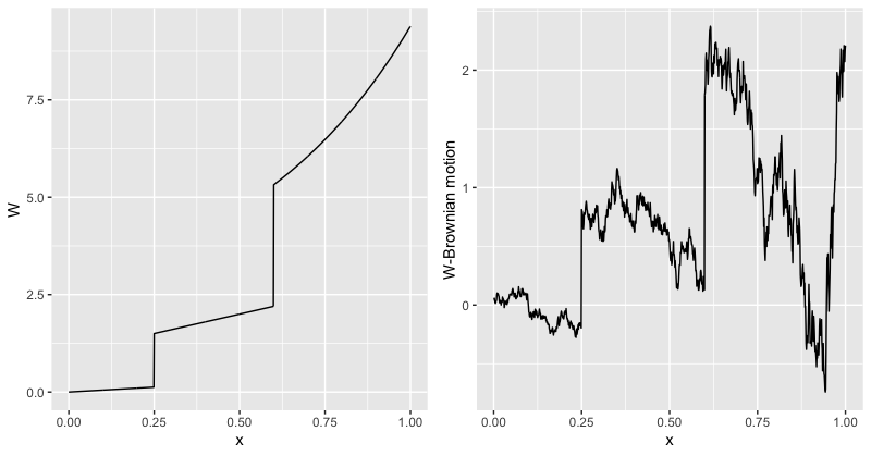
Refer to caption
Figure 1.1: An example of a WW-Brownian motion for a function WW.

We see, on Figure 1.1, an example of a realization of a WW-Brownian motion for a function WW. The plot of WW is on the left-hand side and the realization of the WW-Brownian motion is on the right-hand side. We can see that the WW-Brownian motions has two jumps, one at each discontinuity of WW.

Proposition 1.6.3.

The WW-Brownian motion in law exists.

Proof.

It is an immediate consequence of Kolmogorov’s extension theorem. ∎

Remark 1.6.4.

Notice that if t∗t^{\ast} is a discontinuity point of WW, then there exists some ε>0\varepsilon>0 such that for every h>0h>0,

P⁡(|BW​(t∗−h)−BW​(t∗)|>0)≥ε.P(|B_{W}(t^{\ast}-h)-B_{W}(t^{\ast})|>0)\geq\varepsilon.

Indeed, it is enough to take any ε>0\varepsilon>0 such that P(|N(0,ΔW(t∗)|>0)>εP(|N(0,\Delta W(t^{\ast})|>0)>\varepsilon, where Δ​W​(t∗)=W⁡(t∗)−W⁡(t∗−)\Delta W(t^{\ast})=W(t^{\ast})-W(t^{\ast}-).

Remark 1.6.5.

The previous remark then implies that BWB_{W} is not continuous in probability so, in particular, BWB_{W} is not an additive process (see, for instance, [27] for a definition of additive processes).

Proposition 1.6.6.

If BW​(⋅)B_{W}(\cdot) is a WW-Brownian motion in law, then it is a martingale.

Proof.

By Condition 3 of Definition 1.6.1, E⁡(BW​(t)−BW​(s))=0E(B_{W}(t)-B_{W}(s))=0, and by Condition 2 of 1.6.1, we have that, for t>st>s,

E⁡(BW​(t)|σ⁡(BW​(u),u≤s))\displaystyle E(B_{W}(t)|\sigma(B_{W}(u),u\leq s)) =\displaystyle= E⁡(BW​(t)−BW​(s)|σ⁡(BW​(u),u≤s))+BW​(s)\displaystyle E(B_{W}(t)-B_{W}(s)|\sigma(B_{W}(u),u\leq s))+B_{W}(s)
=\displaystyle= E⁡(BW​(t)−BW​(s))+BW​(s)\displaystyle E(B_{W}(t)-B_{W}(s))+B_{W}(s)
=\displaystyle= BW​(s).\displaystyle B_{W}(s).

∎

Proposition 1.6.7.

The WW-Brownian motion exists.

Proof.

Let BW​(⋅)B_{W}(\cdot) be a WW-Brownian motion in law. We need to show that there exists a càdlàg modification of BW​(⋅)B_{W}(\cdot). To this end, begin by noticing that since BW​(⋅)B_{W}(\cdot) is a martingale, it is a quasimartingale in the sense of [4]. Indeed, see, for instance, claim A.3.2 in [4].

Notice that since the WW-Brownian motion is a ℝ\mathbb{R}-valued quasimartingale, the assumptions of Theorem 2.1 in [4] are satisfied. Thus, in order to apply Theorem 2.1 of [4] to conclude that BW​(⋅)B_{W}(\cdot) has a càdlàg modification, it is enough to show that BW​(⋅)B_{W}(\cdot) is right-continuous in probability.

To such an end, notice that, for t>st>s,

P⁡(|BW​(t)−BW​(s)|>ε)\displaystyle P(|B_{W}(t)-B_{W}(s)|>\varepsilon) ≤\displaystyle\leq E⁡(|BW​(t)−BW​(s)|2)ε2\displaystyle\frac{E\left(\left|B_{W}(t)-B_{W}(s)\right|^{2}\right)}{\varepsilon^{2}}
=\displaystyle= W⁡(t)−W⁡(s)ε2.\displaystyle\frac{W(t)-W(s)}{\varepsilon^{2}}.

Therefore, since WW is right-continuous, BW​(⋅)B_{W}(\cdot) is right-continuous in probability. The result now follows from applying Theorem 2.1 from [4]. ∎

If WW has finitely many discontinuity points and WW is Hölder continuous on each continuous subinterval of the form [di,di+1)[d_{i},d_{i+1}), where {di;i=1,…,N}\{d_{i};i=1,\ldots,N\} is the set of discontinuity points, where N∈ℕN\in\mathbb{N}, then the set of discontinuity points of the sample paths will be contained in the set of discontinuity points of WW:

Proposition 1.6.8.

If the set of discontinuity points of WW is finite, say 0≤d1<d2<…<dN0\leq d_{1}<d_{2}<\ldots<d_{N}, for some n∈ℕn\in\mathbb{N}, and if we let I1=[0,d1),I2=[d1,d2),…,IN=[dN−1,dN),IN+1=[dN,1)I_{1}=[0,d_{1}),I_{2}=[d_{1},d_{2}),\ldots,I_{N}=[d_{N-1},d_{N}),I_{N+1}=[d_{N},1), and for each interval IkI_{k}, there exists some γk∈(0,1]\gamma_{k}\in(0,1], such that the restriction of WW to IkI_{k} is γk\gamma_{k}-Hölder continuous, then BWB_{W} has a modification whose sample paths are continuous on each interval Ik,k=1,…,N+1I_{k},k=1,\ldots,N+1.

Proof.

In this case, we can directly apply Kolmogorov-Chentsov’s continuity theorem to the restriction of BWB_{W} to each interval IkI_{k} to obtain that the restriction of BWB_{W} to each IkI_{k} has a modification, say BW,kB_{W,k}, which has continuous sample paths, for k=1,…,N+1k=1,\ldots,N+1. Notice that from the very construction, the modifications belong to the same probability space. Therefore, we can simply define the modification B~W\widetilde{B}_{W} on 𝕋\mathbb{T} as B~W​(s)=BW,k​(s)\widetilde{B}_{W}(s)=B_{W,k}(s) is s∈Iks\in I_{k}, k=1,…,N+1k=1,\ldots,N+1, and since the intervals IkI_{k} are disjoint, there are no overlaps. ∎

Remark 1.6.9.

It is important to notice that if we only assume WW to have finitely many discontinuity points, and impose no assumptions regarding Hölder continuity, we would only have that the restriction of BWB_{W} to each continuity subinterval is continuous in probability, which implies that the restriction of BWB_{W} to each subinterval is an additive process in law, and thus admits a version which is right-continuous, but is not strong enough to ensure the existence of a modification with continuous sample paths. Thus, we would not be able to conclude that BWB_{W} would be continuous in each interval such that WW is continuous.

Notice that, almost surely, the sample paths of BW​(⋅)B_{W}(\cdot) are bounded on [0,1)[0,1), since it is càdlàg on [0,1)[0,1). Therefore, it is an LV2​(𝕋)L_{V}^{2}(\mathbb{T})-process (and also an LW2​(𝕋)L^{2}_{W}(\mathbb{T})-process). Furthermore, BW​(⋅)B_{W}(\cdot) has orthogonal increments and is L2L^{2}-right-continuous, that is

limt→s+𝔼⁡((BW​(t)−BW​(s))2)=0.\lim_{t\to s+}\mathbb{E}((B_{W}(t)-B_{W}(s))^{2})=0.

Therefore, the definition of the stochastic integral of any function f∈LV2​(𝕋)f\in L^{2}_{V}(\mathbb{T}) with respect to BW​(⋅)B_{W}(\cdot) follows from the standard theory on L2L^{2}-processes (see [2]). Namely, the stochastic integral is linear,

∫[0,1)1(a,b]​d​BW=BW​(b)−BW​(a),\int_{[0,1)}\textbf{1}_{(a,b]}dB_{W}=B_{W}(b)-B_{W}(a), (1.40)

and, for any f∈LW2​(𝕋)f\in L^{2}_{W}(\mathbb{T}), we have the following isometry:

𝔼⁡[(∫[0,1)f​d​BW)2]=∫[0,1)f2​𝑑V.\mathbb{E}\left[\left(\int_{[0,1)}fdB_{W}\right)^{2}\right]=\int_{[0,1)}f^{2}dV. (1.41)

Now, observe that, by (1.40), the integral of each simple function follows a normal distribution. By (1.41), the stochastic integral with respect to BWB_{W} is an L2L^{2}-limit of Gaussian random variables, and thus, it is a Gaussian random variable (see [2, Theorem 1.4.2 ]).

Since, for each simple function φ\varphi, we have 𝔼⁡(∫[0,1)φ​d​BW)=0\mathbb{E}\left(\int_{[0,1)}\varphi dB_{W}\right)=0, it follows from (1.41) that the stochastic integral with respect to any deterministic function f∈LV2​(𝕋)f\in L^{2}_{V}(\mathbb{T}) is zero. Furthermore, since the stochastic integral with respect to deterministic functions is a mean zero Gaussian random variable, it follows from (1.41), again, that for any f∈LV2​(𝕋)f\in L^{2}_{V}(\mathbb{T}),

∫[0,1)f​d​BW∼N⁡(0,∫[0,1)f2​𝑑V).\int_{[0,1)}fdB_{W}\sim N\left(0,\int_{[0,1)}f^{2}dV\right). (1.42)

We can now show that the integration by parts formula can be applied for any function in HW,V​(𝕋)H_{W,V}(\mathbb{T}) and with the derivative, being the weak derivative DW−D_{W}^{-}:

Proposition 1.6.10.

Let BW​(⋅)B_{W}(\cdot) be a WW-Brownian motion. For any g∈HW,V​(𝕋)g\in H_{W,V}(\mathbb{T}) we have the following integration by parts formula:

∫(0,t]g​d​BW=BW​(t)​g​(t)−∫(0,t]BW​(s−)​DW−​g​(s)​𝑑W​(s).\int_{(0,t]}gdB_{W}=B_{W}(t)g(t)-\int_{(0,t]}B_{W}(s-)D_{W}^{-}{g}(s)dW(s). (1.43)
Proof.

Let g∈HW,V​(𝕋)g\in H_{W,V}(\mathbb{T}). From Theorem 1.2.3 and stochastic Fubini’s theorem (see [26, Theorem 64, p.210]), we have

∫(0,t]g​d​BW\displaystyle\int_{(0,t]}gdB_{W} =∫(0,t](g⁡(0)+∫(0,s]DW−​g​(u)​𝑑W​(u))​d​BW​(s)\displaystyle=\int_{(0,t]}\left(g(0)+\int_{(0,s]}D_{W}^{-}g(u)dW(u)\right)dB_{W}(s)
=g⁡(0)​BW​(t)+∫(0,t]DW−​g​(u)​(∫[u,t]d​BW​(s))​𝑑W​(u)\displaystyle=g(0)B_{W}(t)+\int_{(0,t]}D_{W}^{-}g(u)\left(\int_{[u,t]}dB_{W}(s)\right)dW(u)
=g⁡(0)​BW​(t)+∫(0,t]DW−​g​(u)​(BW​(t)−BW​(u−))​𝑑W​(u)\displaystyle=g(0)B_{W}(t)+\int_{(0,t]}D_{W}^{-}g(u)(B_{W}(t)-B_{W}(u-))dW(u)
=g⁡(0)​BW​(t)+BW​(t)​(g⁡(t)−g⁡(0))−∫(0,t]DW−​g​(u)​BW​(u−)​𝑑W​(u)\displaystyle=g(0)B_{W}(t)+B_{W}(t)(g(t)-g(0))-\int_{(0,t]}D_{W}^{-}g(u)B_{W}(u-)dW(u)
=BW​(t)​g​(t)−∫(0,t]DW−​g​(u)​BW​(u−)​𝑑W​(u).\displaystyle=B_{W}(t)g(t)-\int_{(0,t]}D_{W}^{-}g(u)B_{W}(u-)dW(u).

∎

Notice that since BW​(⋅)B_{W}(\cdot) has càdlàg sample paths, BW​(⋅)B_{W}(\cdot) is almost surely bounded on 𝕋\mathbb{T}, so the right-hand side of (1.43) is well-defined.

We will now obtain the Cameron-Martin space of the WW-Brownian motion. The Cameron-Martin spaces appear naturally on Malliavin calculus as the set of "directions" in which one can differentiate (with respect to the Malliavin derivative). Recently Bolin and Kirchner [19] showed that the Cameron-Martin spaces play a key role in find the best linear predictor with the "wrong" covariance structure. More generally, the Cameron-Martin space uniquely determines the Gaussian measure (see [5, Theorem 2.9]) on Banach spaces. Furthermore, the Cameron-Martin space is, in a sense, independent of the Banach space in which the Gaussian measure is defined (see [5, Proposition 2.10]). This means that one can specify a Gaussian measure by specifing the Cameron-Martin space. This means that, by computing the Cameron-Martin space of BWB_{W}, we are showing that the distribution of WW-Brownian motion in LV2​(𝕋)L^{2}_{V}(\mathbb{T}) is the unique Gaussian measure associated to the Sobolev space HW,V,𝒟​(𝕋)H_{W,V,\mathcal{D}}(\mathbb{T}).

We begin by noting that from Example 2.3.16 in Bogachev [3], since the WW-Brownian motion has càdlàg sample paths, and

∫[0,1)W⁡(t)​𝑑V​(t)≤W⁡(1)​V​(1)<∞,\int_{[0,1)}W(t)dV(t)\leq W(1)V(1)<\infty,

we have that the distribution of BWB_{W} on LV2​(𝕋)L^{2}_{V}(\mathbb{T}), i.e., the measure given by

γW(B)=ℙ(ω:BW(⋅,ω)∈B),\gamma_{W}(B)=\mathbb{P}\left(\omega:B_{W}(\cdot,\omega)\in B\right),

where BB is a borel set in LV2​(𝕋)L^{2}_{V}(\mathbb{T}) (which is a separable Hilbert space), defines a Gaussian measure in LV2​(𝕋)L^{2}_{V}(\mathbb{T}).

Let K:LV2​(𝕋)→LV2​(𝕋)K:L^{2}_{V}(\mathbb{T})\to L^{2}_{V}(\mathbb{T}) be the covariance operator of BW​(⋅)B_{W}(\cdot), i.e., of the Gaussian measure induced by BW​(⋅)B_{W}(\cdot) in LV2​(𝕋)L^{2}_{V}(\mathbb{T}). Since LV2​(𝕋)L^{2}_{V}(\mathbb{T}) is a Hilbert space, we can apply Theorem 2.3.1 in Bogachev [3] to obtain that the Fourier transform of γW\gamma_{W} satisfies, for every g∈LV2​(𝕋)g\in L^{2}_{V}(\mathbb{T}),

γ^W​(g)=∫LV2​(𝕋)ei​⟨g,f⟩LV2​(𝕋)​d​γW​(f)=exp⁡{−12​⟨K​g,g⟩LV2​(𝕋)}.\widehat{\gamma}_{W}(g)=\int_{L^{2}_{V}(\mathbb{T})}e^{i\langle g,f\rangle_{L^{2}_{V}(\mathbb{T})}}d\gamma_{W}(f)=\exp\left\{-\frac{1}{2}\langle Kg,g\rangle_{L^{2}_{V}(\mathbb{T})}\right\}. (1.44)

We will then compute the Fourier transform (1.44) explicitly to show that KK is a kernel operator and its kernel is, indeed, the covariance function of the WW-Brownian motion. To such an end, by standard limiting arguments, it is enough to show the result for simple functions. We will provide the details for the case of indicator functions of intervals of the form (a,b](a,b]. The case of linear combination of indicators functions can be carried out similarly. Let us consider then, the function 1(a,b]\textbf{1}_{(a,b]}. By using stochastic Fubini’s theorem (see [26, Theorem 64, p.210]), we have

γ^W​(1(a,b])\displaystyle\widehat{\gamma}_{W}(\textbf{1}_{(a,b]}) =∫LV2​(𝕋)exp⁡{i​⟨1(a,b],f⟩LV2​(𝕋)}=𝔼⁡[exp⁡{i​∫(a,b]BW​(s)​𝑑V​(s)}]\displaystyle=\int_{L^{2}_{V}(\mathbb{T})}\exp\left\{i\langle\textbf{1}_{(a,b]},f\rangle_{L^{2}_{V}(\mathbb{T})}\right\}=\mathbb{E}\left[\exp\left\{i\int_{(a,b]}B_{W}(s)dV(s)\right\}\right]
=𝔼⁡[exp⁡{i​∫(a,b]∫(0,s]d​BW​(u)​𝑑V​(s)}]\displaystyle=\mathbb{E}\left[\exp\left\{i\int_{(a,b]}\int_{(0,s]}dB_{W}(u)dV(s)\right\}\right]
=𝔼⁡[exp⁡{i​∫(0,a]∫(a,b]d​V​(s)​d​BW​(u)+i​∫(a,b]∫[u,b]d​V​(s)​d​BW​(u)}]\displaystyle=\mathbb{E}\left[\exp\left\{i\int_{(0,a]}\int_{(a,b]}dV(s)dB_{W}(u)+i\int_{(a,b]}\int_{[u,b]}dV(s)dB_{W}(u)\right\}\right]
=𝔼⁡[exp⁡{i⁡(V⁡(b+)−V⁡(a+))​BW​(a)+i​∫(a,b](V⁡(b+)−V⁡(u))​d​BW​(u)}]\displaystyle=\mathbb{E}\left[\exp\left\{i(V(b+)-V(a+))B_{W}(a)+i\int_{(a,b]}(V(b+)-V(u))dB_{W}(u)\right\}\right]
=exp⁡{−12​[W⁡(a)​(V⁡(b+)−V⁡(a+))2+∫(a,b](V⁡(b+)−V⁡(u))2​𝑑W]},\displaystyle=\exp\left\{-\frac{1}{2}\left[W(a)(V(b+)-V(a+))^{2}+\int_{(a,b]}(V(b+)-V(u))^{2}dW\right]\right\},

where in the last expression we used the fact that the increments are independent, the characteristic function of a normal distribution and the distribution of the stochastic integrals (1.42). In order to show that KK is a kernel operator with kernel k⁡(s,t)=W⁡(t∧s)k(s,t)=W(t\land s), we need to show that if we take K^:LV2​(𝕋)→LV2​(𝕋)\widehat{K}:L^{2}_{V}(\mathbb{T})\to L^{2}_{V}(\mathbb{T}), defined by

K^​f​(t)=∫[0,1)W⁡(t∧s)​f​(s)​𝑑V​(s).\widehat{K}f(t)=\int_{[0,1)}W(t\land s)f(s)dV(s). (1.45)

Then,

⟨K^​1(a,b],1(a,b]⟩LV2​(𝕋)=W⁡(a)​(V⁡(b+)−V⁡(a+))2+∫(a,b](V⁡(b+)−V⁡(u))2​𝑑W.\langle\widehat{K}\textbf{1}_{(a,b]},\textbf{1}_{(a,b]}\rangle_{L^{2}_{V}(\mathbb{T})}=W(a)(V(b+)-V(a+))^{2}+\int_{(a,b]}(V(b+)-V(u))^{2}dW. (1.46)

Let us then show that the above expression is true. We have,

∫[0,1)∫[0,1)W⁡(t∧s)​1(a,b]​(t)​1(a,b]​(s)​𝑑V​(t)​𝑑V​(s)\displaystyle\int_{[0,1)}\int_{[0,1)}W(t\land s)\textbf{1}_{(a,b]}(t)\textbf{1}_{(a,b]}(s)dV(t)dV(s) =∫(a,b]∫(a,b]W⁡(t∧s)​𝑑V​(t)​𝑑V​(s)\displaystyle=\int_{(a,b]}\int_{(a,b]}W(t\land s)dV(t)dV(s)
=∫(a,b]∫(a,s]W⁡(t)​𝑑V​(t)​𝑑V​(s)+\displaystyle=\int_{(a,b]}\int_{(a,s]}W(t)dV(t)dV(s)+
+∫(a,b]∫(s,b]W(s)dV(t)dV(s).\displaystyle+\int_{(a,b]}\int_{(s,b]}W(s)dV(t)dV(s).

The last expression is equal to

∫(a,b](∫(a,s]∫(0,t]d​W​(u)​𝑑V​(t)+∫(s,b]∫(0,s]d​W​(u)​𝑑V​(t))​𝑑V​(s),\int_{(a,b]}\left(\int_{(a,s]}\int_{(0,t]}dW(u)dV(t)+\int_{(s,b]}\int_{(0,s]}dW(u)dV(t)\right)dV(s),

which, by Fubini’s theorem, can be written as

∫(0,b](∫(a,b]∫(a,b](1(0,t]​(u)​1(a,s]​(t)​1(a,b]​(s)+1(0,b]​(u)​1(s,b]​(t)​1(a,b]​(s))​𝑑V​(t)​𝑑V​(s))​𝑑W​(u).\int_{(0,b]}\left(\int_{(a,b]}\int_{(a,b]}\left(\textbf{1}_{(0,t]}(u)\textbf{1}_{(a,s]}(t)\textbf{1}_{(a,b]}(s)+\textbf{1}_{(0,b]}(u)\textbf{1}_{(s,b]}(t)\textbf{1}_{(a,b]}(s)\right)dV(t)dV(s)\right)dW(u).

Let us split the integral with respect to d​W​(u)dW(u) into two parts, one for u≤au\leq a, and the other when u>au>a. The integral over of d​W​(u)dW(u) over (0,a](0,a] is equal to

∫(0,a]((1(a,s]​(t)​1(a,b]​(s)+1(s,b]​(t)​1(a,b]​(s))​𝑑V​(t)​𝑑V​(s))​𝑑W​(u),\int_{(0,a]}\left((\textbf{1}_{(a,s]}(t)\textbf{1}_{(a,b]}(s)+\textbf{1}_{(s,b]}(t)\textbf{1}_{(a,b]}(s))dV(t)dV(s)\right)dW(u),

and thus, equal to

∫(0,a]∫(a,b]∫(a,b]1(a,b]​(t)​1(a,b]​(s)​𝑑V​(t)​𝑑V​(s)​𝑑W​(u)=W⁡(a)​(V⁡(b+)−V⁡(a+))2.\int_{(0,a]}\int_{(a,b]}\int_{(a,b]}\textbf{1}_{(a,b]}(t)\textbf{1}_{(a,b]}(s)dV(t)dV(s)dW(u)=W(a)(V(b+)-V(a+))^{2}.

This is the first part of (1.46). Let us now compute the integral with respect to d​W​(u)dW(u) over (a,b](a,b]:

∫(a,b]∫(a,b]∫(a,b](1(a,t]​(u)​1(a,s]​(t)​1(a,b]​(s)+1(a,b]​(u)​1(s,b]​(t)​1(a,b]​(s))​𝑑V​(t)​𝑑V​(s)​𝑑W​(u).\int_{(a,b]}\int_{(a,b]}\int_{(a,b]}\left(\textbf{1}_{(a,t]}(u)\textbf{1}_{(a,s]}(t)\textbf{1}_{(a,b]}(s)+\textbf{1}_{(a,b]}(u)\textbf{1}_{(s,b]}(t)\textbf{1}_{(a,b]}(s)\right)dV(t)dV(s)dW(u).

To such an end, observe that:

1(a,t]​(u)​1(a,s]​(t)​1(a,b]​(s)=1(a,b]​(u)​1[u,b]​(s)​1[u,s]​(t)\textbf{1}_{(a,t]}(u)\textbf{1}_{(a,s]}(t)\textbf{1}_{(a,b]}(s)=\textbf{1}_{(a,b]}(u)\textbf{1}_{[u,b]}(s)\textbf{1}_{[u,s]}(t)

and

1(a,b]​(u)​1(s,b]​(t)​1(a,b]​(s)=1(a,b]​(u)​1[u,b]​(s)​1(s,b]​(t).\textbf{1}_{(a,b]}(u)\textbf{1}_{(s,b]}(t)\textbf{1}_{(a,b]}(s)=\textbf{1}_{(a,b]}(u)\textbf{1}_{[u,b]}(s)\textbf{1}_{(s,b]}(t).

By summing both expressions above, we arrive at

1(a,t]​(u)​1(a,s]​(t)​1(a,b]​(s)+1(a,b]​(u)​1(s,b]​(t)​1(a,b]​(s)=1(a,b]​(u)​1[u,b]​(s)​1[u,b]​(t).\textbf{1}_{(a,t]}(u)\textbf{1}_{(a,s]}(t)\textbf{1}_{(a,b]}(s)+\textbf{1}_{(a,b]}(u)\textbf{1}_{(s,b]}(t)\textbf{1}_{(a,b]}(s)=\textbf{1}_{(a,b]}(u)\textbf{1}_{[u,b]}(s)\textbf{1}_{[u,b]}(t).

Therefore, the resulting integral is

∫(a,b]∫(a,b]∫(a,b]1(a,b]​(u)​1[u,b]​(s)​1[u,b]​(t)​𝑑V​(t)​𝑑V​(s)​𝑑W​(u)=∫(a,b](V⁡(b+)−V⁡(u))2​𝑑W​(u).\int_{(a,b]}\int_{(a,b]}\int_{(a,b]}\textbf{1}_{(a,b]}(u)\textbf{1}_{[u,b]}(s)\textbf{1}_{[u,b]}(t)dV(t)dV(s)dW(u)=\int_{(a,b]}(V(b+)-V(u))^{2}dW(u).

This is the second expression in (1.46) and completes the proof for the case of indicator functions. As mentioned previously, the case of linear combinations of indicator functions follows similarly. So, the covariance operator of BW​(⋅)B_{W}(\cdot) is, indeed, a kernel operator in LV2​(𝕋)L^{2}_{V}(\mathbb{T}) with kernel k⁡(t,s)=W⁡(t∧s).k(t,s)=W(t\land s).

We will now obtain the Cameron-Martin space associated to the WW-Brownian motion. To such an end, recall that the covariance operator of the WW-Brownian motion was given in (1.45). Let us now obtain a nicer expression for K^​f\widehat{K}f using Fubini’s theorem:

K^​f​(t)\displaystyle\widehat{K}f(t) =∫[0,1)W⁡(t∧s)​f​(s)​𝑑V​(s)=∫[0,t)W⁡(s)​f​(s)​𝑑V​(s)+∫[t,1)W⁡(t)​f​(s)​𝑑V​(s)\displaystyle=\int_{[0,1)}W(t\land s)f(s)dV(s)=\int_{[0,t)}W(s)f(s)dV(s)+\int_{[t,1)}W(t)f(s)dV(s)
=∫[0,t)∫(0,s]d​W​(u)​f​(s)​𝑑V​(s)+∫[t,1)∫(0,t]d​W​(u)​f​(s)​𝑑V​(s)\displaystyle=\int_{[0,t)}\int_{(0,s]}dW(u)f(s)dV(s)+\int_{[t,1)}\int_{(0,t]}dW(u)f(s)dV(s)
=∫(0,t]∫[u,t)f⁡(s)​𝑑V​(s)​𝑑W​(u)+∫(0,t]∫[t,1)f⁡(s)​𝑑V​(s)​𝑑W​(u)\displaystyle=\int_{(0,t]}\int_{[u,t)}f(s)dV(s)dW(u)+\int_{(0,t]}\int_{[t,1)}f(s)dV(s)dW(u)
=∫(0,t]∫[u,1)f⁡(s)​𝑑V​(s)​𝑑W​(u)\displaystyle=\int_{(0,t]}\int_{[u,1)}f(s)dV(s)dW(u)
=W⁡(t)​∫[0,1)f⁡(s)​𝑑V​(s)−∫(0,t]∫[0,u)f⁡(s)​𝑑V​(s)​𝑑W​(u).\displaystyle=W(t)\int_{[0,1)}f(s)dV(s)-\int_{(0,t]}\int_{[0,u)}f(s)dV(s)dW(u). (1.47)

Thus, K^​(f)​(t)=W⁡(t)​∫[0,1)f⁡(s)​𝑑V​(s)−∫(0,t]∫[0,u)f⁡(s)​𝑑V​(s)​𝑑W​(u)\widehat{K}(f)(t)=W(t)\int_{[0,1)}f(s)dV(s)-\int_{(0,t]}\int_{[0,u)}f(s)dV(s)dW(u). So, in particular, K^​(f)​(0)=0\widehat{K}(f)(0)=0 and the WW-left-derivative of K^​(f)\widehat{K}(f) given by

DW−​(K^​f)​(t)=∫[0,1)f⁡(s)​𝑑V​(s)−∫[0,t)f⁡(s)​𝑑V​(s)D_{W}^{-}(\widehat{K}f)(t)=\int_{[0,1)}f(s)dV(s)-\int_{[0,t)}f(s)dV(s)

satisfies DW−​(K^​f)​(1)=0D_{W}^{-}(\widehat{K}f)(1)=0. This motivates the definition of the subspace of HW,V​(𝕋)H_{W,V}(\mathbb{T}) with a tagged zero, and Dirichlet boundary conditions at zero:

HW,V,𝒟​(𝕋)={f∈HW,V​(𝕋)∩LV,02​(𝕋):f⁡(0)=0}.H_{W,V,\mathcal{D}}(\mathbb{T})=\left\{f\in H_{W,V}(\mathbb{T})\cap L^{2}_{V,0}(\mathbb{T}):f(0)=0\right\}.

Note that in this space, the following is an equivalent norm to the Sobolev norm (denote by ⟨⋅,⋅⟩W,V,𝒟\langle\cdot,\cdot\rangle_{W,V,\mathcal{D}} the inner product associated to this norm):

‖f‖W,V,𝒟2=∫𝕋(DW−​f)2​𝑑W.\|f\|_{W,V,\mathcal{D}}^{2}=\int_{\mathbb{T}}(D_{W}^{-}f)^{2}dW.

Indeed, on one hand we always have for any f∈HW,V​(𝕋)f\in H_{W,V}(\mathbb{T}), ‖f‖W,V,𝒟≤‖f‖W,V\|f\|_{W,V,\mathcal{D}}\leq\|f\|_{W,V}. On the other hand, from Theorem 1.2.3, it follows from the elementary inequality (a+b)2≤2​(a2+b2)(a+b)^{2}\leq 2(a^{2}+b^{2}) and Jensen’s inequality that there exists some constant C>0C>0 such that

‖f‖LV2​(𝕋)2≤C⁡((f⁡(0))2+‖DW−​f‖LW2​(𝕋)2).\|f\|^{2}_{L^{2}_{V}(\mathbb{T})}\leq C\left((f(0))^{2}+\|D_{W}^{-}f\|_{L^{2}_{W}(\mathbb{T})}^{2}\right).

Let us now show that the Cameron-Martin space of the WW-Brownian motion on LV2​(𝕋)L^{2}_{V}(\mathbb{T}) is, indeed, HW,V,𝒟​(𝕋)H_{W,V,\mathcal{D}}(\mathbb{T}). We know that the Cameron-Martin space of the WW-Brownian motion is given by ℋ=K^1/2​(LV2​(𝕋))\mathcal{H}=\widehat{K}^{1/2}(L^{2}_{V}(\mathbb{T})), since K^\widehat{K} is the covariance operator of the WW-Brownian motion on LV2​(𝕋)L^{2}_{V}(\mathbb{T}). Equivalently, ℋ\mathcal{H} is the completion of K^​(LV2​(𝕋))\widehat{K}(L^{2}_{V}(\mathbb{T})) relative to the norm ∥⋅∥ℋ=⟨K^(⋅),⋅⟩LW2​(𝕋)\|\cdot\|_{\mathcal{H}}=\left\langle\widehat{K}(\cdot),\cdot\right\rangle_{L^{2}_{W}(\mathbb{T})}. Now, we will see that in the K^​(LV2​(𝕋))\widehat{K}(L^{2}_{V}(\mathbb{T})) the norm ∥⋅∥K^\|\cdot\|_{\widehat{K}} is well know. In fact, given f,g∈K^​(LV2​(𝕋))f,g\in\widehat{K}(L^{2}_{V}(\mathbb{T})) there exist functions u,v∈LV2​(𝕋)u,v\in L^{2}_{V}(\mathbb{T}) such that f=K^​uf=\widehat{K}u and g=K^​vg=\widehat{K}v. Hence, let h⁡(w)=∫[w,1)u⁡(t)​𝑑V​(t)h(w)=\int_{[w,1)}u(t)dV(t), so, by Fubini’s theorem and 1.6,

⟨f,g⟩ℋ\displaystyle\langle f,g\rangle_{\mathcal{H}} =⟨K^​u,v⟩LV2​(𝕋)\displaystyle=\langle\widehat{K}u,v\rangle_{L^{2}_{V}(\mathbb{T})}
=∫[0,1)(∫(0,s]∫[w,1)u⁡(t)​𝑑V​(t)​𝑑W​(w))​v​(s)​𝑑V​(s)\displaystyle=\int_{[0,1)}\left(\int_{(0,s]}\int_{[w,1)}u(t)dV(t)dW(w)\right)v(s)dV(s)
=∫[0,1)∫[0,s)h⁡(w)​v​(s)​𝑑W​(w)​𝑑V​(s)=∫[0,1)h⁡(w)​(∫[w,1)v⁡(s)​𝑑V​(s))​𝑑W​(w)\displaystyle=\int_{[0,1)}\int_{[0,s)}h(w)v(s)dW(w)dV(s)=\int_{[0,1)}h(w)\left(\int_{[w,1)}v(s)dV(s)\right)dW(w)
=∫[0,1)(∫[w,1)u⁡(s)​𝑑V​(s))​(∫[w,1)v⁡(s)​𝑑V​(s))​𝑑W​(w)\displaystyle=\int_{[0,1)}\left(\int_{[w,1)}u(s)dV(s)\right)\left(\int_{[w,1)}v(s)dV(s)\right)dW(w)
=⟨DW−​f,DW−​g⟩LW2​(𝕋)=⟨f,g⟩W,V,𝒟.\displaystyle=\langle D_{W}^{-}f,D_{W}^{-}g\rangle_{L^{2}_{W}(\mathbb{T})}=\langle f,g\rangle_{W,V,\mathcal{D}}.

This shows that the Cameron-Martin norm is given by ∥⋅∥W,V,𝒟\|\cdot\|_{W,V,\mathcal{D}}. Finally, a straightforward adaptation of Theorem 1.1.7 shows that K^​(LV2​(𝕋))\widehat{K}(L^{2}_{V}(\mathbb{T})), is dense in the space HW,V,𝒟​(𝕋)H_{W,V,\mathcal{D}}(\mathbb{T}). Therefore, since the Cameron-Martin space is the completion of K^​(LV2​(𝕋))⊂HW,V,𝒟​(𝕋)\widehat{K}(L^{2}_{V}(\mathbb{T}))\subset H_{W,V,\mathcal{D}}(\mathbb{T}) with respect to the norm ∥⋅∥W,V,𝒟\|\cdot\|_{W,V,\mathcal{D}} we have that ℋ=HW,V,𝒟​(𝕋)\mathcal{H}=H_{W,V,\mathcal{D}}(\mathbb{T}).

Remark 1.6.11.

It is interesting to observe that since we looked at the WW-Brownian motion as an element of LV2​(𝕋)L^{2}_{V}(\mathbb{T}), we were able to show that its Cameron-Martin space is HW,V​(𝕋)H_{W,V}(\mathbb{T}). It is clear that we can embed the WW-Brownian motion into other LV~2​(𝕋)L_{\widetilde{V}}^{2}(\mathbb{T}) spaces. Indeed, since 𝕋\mathbb{T} is compact and the sample paths of the WW-Brownian motion are càdlàg, they are bounded, so belong to any LV~2​(𝕋)L_{\widetilde{V}}^{2}(\mathbb{T}), where V~:ℝ→ℝ\widetilde{V}:\mathbb{R}\to\mathbb{R} is increasing and periodic in the sense of (1.2). This shows that the VV is not very important for the WW-Brownian motion, what really matters is the WW and it is reflected at its Cameron-Martin space, HW,V,𝒟​(𝕋)H_{W,V,\mathcal{D}}(\mathbb{T}). In HW,V,𝒟​(𝕋)H_{W,V,\mathcal{D}}(\mathbb{T}), the weak derivative in WW is the true restriction, since by Theorem 1.2.3, we have HW,V,𝒟​(𝕋)⊂LV~2​(𝕋)H_{W,V,\mathcal{D}}(\mathbb{T})\subset L_{\widetilde{V}}^{2}(\mathbb{T}). This is in consonance with the Cameron-Martin space uniquely determining the Gaussian measure. Indeed, the VV function does not have much impact on the WW-Brownian motion, and also, does not have much impact on its Cameron-Martin space, in the sense that it is contained on any LV~2​(𝕋)L_{\widetilde{V}}^{2}(\mathbb{T}).

1.7 Applications to stochastic partial differential equations

We will now apply the theory to solve a class of stochastic partial differential equations that generalize a non-fractional case of the well-known Matérn equations on a domain with periodic boundary conditions.

For this section, we will work on HW,V,𝒟​(𝕋)H_{W,V,\mathcal{D}}(\mathbb{T}) with a tagged zero and, furthermore, recall that we assumed that WW is continuous at x=0x=0. Therefore, from Theorem 1.2.3, we have that for any function g∈HW,V​(𝕋)g\in H_{W,V}(\mathbb{T}),

limx→1−g⁡(x)=g⁡(0)=limx→0+g⁡(x).\lim_{x\to 1-}g(x)=g(0)=\lim_{x\to 0+}g(x).

This means that if g∈HW,V,𝒟​(𝕋),g\in H_{W,V,\mathcal{D}}(\mathbb{T}),

limx→1−g⁡(x)=0=limx→0+g⁡(x).\lim_{x\to 1-}g(x)=0=\lim_{x\to 0+}g(x).

Therefore, it follows from the integration by parts formula, (1.43), that under these assumptions, for any g∈HW,V,𝒟​(𝕋),g\in H_{W,V,\mathcal{D}}(\mathbb{T}), we have

∫𝕋g(s)dBW(s)=−∫𝕋BW(s−)DW−g(s)dW(s).\int_{\mathbb{T}}g(s)dB_{W}(s)=-\int_{\mathbb{T}}B_{W}(s-)D_{W}^{-}{g}(s)dW(s).

So that

|∫𝕋g⁡(s)​d​BW​(s)|\displaystyle\left|\int_{\mathbb{T}}g(s)dB_{W}(s)\right| ≤\displaystyle\leq ∫𝕋|BW​(s)​DW−​g​(s)|​𝑑W​(s)\displaystyle\int_{\mathbb{T}}|B_{W}(s)D_{W}^{-}{g}(s)|dW(s) (1.48)
≤\displaystyle\leq ‖BW‖LW2​(𝕋)​‖DW−​g‖LW2​(𝕋)\displaystyle\|B_{W}\|_{L^{2}_{W}(\mathbb{T})}\|D_{W}^{-}g\|_{L^{2}_{W}(\mathbb{T})}
≤\displaystyle\leq (supt∈𝕋‖BW​(t)‖)​W​(1)​‖g‖HW,V​(𝕋).\displaystyle\left(\sup_{t\in\mathbb{T}}\|B_{W}(t)\|\right)W(1)\|g\|_{H_{W,V}(\mathbb{T})}.

So, the stochastic integral defines, almost surely, a bounded linear functional on HW,V,𝒟​(𝕋)H_{W,V,\mathcal{D}}(\mathbb{T}). We can now define the pathwise WW-gaussian white noise on the Cameron-Martin space HW,V,𝒟​(𝕋)H_{W,V,\mathcal{D}}(\mathbb{T}).

Definition 1.7.1.

We define the pathwise WW-gaussian white noise, B˙W∈HW,V,0−1​(𝕋):=(HW,V,𝒟​(𝕋))∗\dot{B}_{W}\in H^{-1}_{W,V,0}(\mathbb{T}):=(H_{W,V,\mathcal{D}}(\mathbb{T}))^{\ast}, as the functional

B˙W(g)=−∫𝕋BW(s)DW−g(s)dW(s).\dot{B}_{W}(g)=-\int_{\mathbb{T}}B_{W}(s)D_{W}^{-}g(s)dW(s). (1.49)

We will now study the existence and uniqueness of weak solutions of the following stochastic partial differential equation:

κ2​u−DV+​(H​DW−​u)=B˙W\kappa^{2}u-D_{V}^{+}(HD_{W}^{-}u)=\dot{B}_{W} (1.50)

on the space HW,V,𝒟​(𝕋)H_{W,V,\mathcal{D}}(\mathbb{T}).

It is important to notice that equation (1.50) can be seen as WW-generalized counterpart of a special non-fractional case of the well-known Matérn stochastic partial differential equation.

Let us now, provide the definition of weak solution of the above equations:

Definition 1.7.2.

We say that u∈HW,V,𝒟​(𝕋)u\in H_{W,V,\mathcal{D}}(\mathbb{T}) is a weak solution of equation (1.50) if for every g∈HW,V,𝒟​(𝕋)g\in H_{W,V,\mathcal{D}}(\mathbb{T}), the following identity is true:

∫𝕋κ2​u​g​𝑑V+∫𝕋H​DW−​u​DW−​g​𝑑W=∫𝕋g​d​BW,\int_{\mathbb{T}}\kappa^{2}ugdV+\int_{\mathbb{T}}HD_{W}^{-}uD_{W}^{-}gdW=\int_{\mathbb{T}}gdB_{W},

or, equivalently, in terms of functionals, if the following identity is true:

BLW,V​(u,g)=B˙W​(g),B_{L_{W,V}}(u,g)=\dot{B}_{W}(g),

where BLW,VB_{L_{W,V}} is the bilinear functional given by

∫𝕋κ2​u​g​𝑑V+∫𝕋H​DW−​u​DW−​g​𝑑W\int_{\mathbb{T}}\kappa^{2}ugdV+\int_{\mathbb{T}}HD_{W}^{-}uD_{W}^{-}gdW

for u,g∈HW,V,𝒟​(𝕋)u,g\in H_{W,V,\mathcal{D}}(\mathbb{T}) and B˙W\dot{B}_{W} is the pathwise WW-Gaussian white noise defined in (1.49).

By comparing with the solutions of the standard Matérn equation, we can readily see that equation (1.7.1) can be suitable for modelling situations in which the process finds barriers, as well as, having eventually non-diffusive behavior throughout the domain (corresponding to situations in which the function WW is continuous, but not Hölder continuous, in some interval).

We, then, have the following theorem on existence and uniqueness of solutions of (1.50):

Theorem 1.7.3.

Let κ\kappa and HH be bounded functions that are also bounded away from zero, where HH is positive. Then, equation (1.50) has a unique solution with, almost surely, càdlàg sample paths.

Proof.

From (1.48), B˙W\dot{B}_{W} is, almost surely, an element of HW,V,0−1​(𝕋)H^{-1}_{W,V,0}(\mathbb{T}). Therefore, from Lax-Milgram theorem, (1.50) has a unique solution. Finally, from Theorem 1.2.3, uu has, almost surely, càdlàg sample paths. ∎

Chapter 2 Fractional one-sided measure theoretic Sobolev spaces, generalized Maclaurin expansion and applications to generalized stochastic partial differential equations

The study of functional equations may lead to problems with solutions that are discontinuous. One natural question is regarding the regularity of such discontinuous functions in some sense. This motivated the definition of a differential operator, in which one differentiates a function with respect to another function that may have discontinuity points. Recently, these differential operators are drawing attention for some researchers. See, for instance,[11, 25, 29, 1, 16] and [15].

Let us illustrate how the discontinuities of the function that induces the differential operator can afftect the solutions of differential equations driven by such operators. Consider, for instance, the equation

ρt−Dx​DW​ϕ​(ρ)=0,\rho_{t}-D_{x}D_{W}\phi(\rho)=0,

which was studied in [15], where DxD_{x} is the usual differential operator and DWD_{W} is a differential operator with respect to some right-continuous and strictly increasing function. They showed that this equation can model diffusion on permeable membranes in which the discontinuity nature of the solution is associated to reflection of particles on the discontinuity points of WW. On the other hand, if we turn our attention to impulsive differential equations, for instance,

{Dt​x​(t)=f⁡(x,t);Δ​x​(tk)=Ik​(tk),\begin{cases}D_{t}x(t)=f(x,t);\\ \Delta x(t_{k})=I_{k}(t_{k}),\end{cases}

where Δ​x​(t):=x⁡(t)−x⁡(−t)\Delta{x}(t):=x(t)-x(-t) and {tk}\{t_{k}\} is a finite set of real numbers. Then, the solutions of the above equations naturally present discontinuities due to the moments of impulse. For more details regarding this last equation we refer the reader to [25] and [13].

Based on these problems, [28] purpose the study of the one-sided differential equations with respect to the operator

LW,V:=κ2−DV+​H​DW−,L_{W,V}:=\kappa^{2}-D^{+}_{V}HD^{-}_{W},

where DV+D_{V}^{+} stands for the right-derivative with respect to VV and DW−D_{W}^{-} stands for left-derivative with respect to WW. Both of these operators will be introduced rigorously in the next section. In [28], they also introduced the so-called WW-VV-Sobolev space HW,V​(𝕋)H_{W,V}(\mathbb{T}), which is a natural environment for the solutions of the above equation, under general conditions on κ\kappa and HH. Also in [28], the authors proved the regularity of the eigenvectors associated to the problem

{ΔW,V​u=λ​u;u∈𝒟W,V​(𝕋).\begin{cases}\Delta_{W,V}u=\lambda u;\\ u\in\mathcal{D}_{W,V}(\mathbb{T}).\end{cases} (2.1)

It is important to observe that there is a need for the study of the eigenvalues in the above problem. For instance, in [12], they introduced a space of test functions, which they denoted by 𝒮W​(𝕋d)\mathcal{S}_{W}(\mathbb{T}^{d}), and proved that it is nuclear. However, due to the lack of properties regarding the eigenvalues of the differential operator Dx​DWD_{x}D_{W}, the definition of 𝒮W​(𝕋d)\mathcal{S}_{W}(\mathbb{T}^{d}) became very abstract and artificial.

Furthermore, given a differential operator LL, it is crucial in the study of stochastic partial differential equations to know when the fractional operator L−sL^{-s}, s>0s>0, is trace class or Hilbert-Schmidt. These questions can only be answered by a detailed study on the eigenvalues of the operator LL.

Therefore, the main goal of this work is to provide the tools to study the eigenvalues of the generalized differential operator and, then, obtain sharp estimates of their growth. Let us now describe the remaining of the paper. We begin the paper by recalling some of the results on WW-VV-Sobolev spaces introduced by [28]. Then, we study the space of infinitely differential functions with respect to the operator DV+​DW−D_{V}^{+}D_{W}^{-}, CW,V∞​(𝕋)C^{\infty}_{W,V}(\mathbb{T}), and determine under what conditions a function ff in this space can be represented as

f⁡(x)=∑k=1∞DW,V(n)​f​(0)​Fk​(x),f(x)=\sum_{k=1}^{\infty}D^{(n)}_{W,V}f(0)F_{k}(x),

where the operator DW,V(n)D^{(n)}_{W,V} is obtained by recursively applying the operators DV+D_{V}^{+} and DW−D_{W}^{-}. FkF_{k} can be interpreted as a generalized polynomial. This last result provides us the tools to obtain a series expansion of the eigenvectors of the operator DV+​DW−D_{V}^{+}D_{W}^{-}. By using the representation of the eigenvectors as series, we are able to use some results in complex analysis to obtain a sharp lower bound for the growth of the eigenvalues of the operator DV+​DW−D_{V}^{+}D_{W}^{-}. We, then, introduce the fractional spaces HW,Vs​(𝕋)H^{s}_{W,V}(\mathbb{T}) based on the Fourier characterization of HW,V​(𝕋)H_{W,V}(\mathbb{T}) proved in [28]. At this point we are able to extend the definitions and results to dimension dd by taking tensor products. Finally, we apply the theory to prove existence and uniqueness of solutions of a fractional stochastic partial differential equation that generalizes the well-known Matérn equation when the domain is the dd-dimensional torus.

2.1 WW-VV-Sobolev spaces and the generalized Laplacian

In this section we will briefly recall some definitions and results obtained in [28] with respect to WW-VV-Sobolev spaces. First, we say that a function is càdlàg (from french, “continue à droite, limite à gauche”) if the function is right-continuous and has limits from the left. Similarly, we say that a function is càglàd, if the function is left-continuous and has limits from the right.

Fix two strictly increasing functions W,V:𝕋→𝕋W,V:\mathbb{T}\to\mathbb{T}, with WW being càdlàg and VV being càglàd. We also assume they satisfy the following periodic conditions :

∀x∈ℝ,{W⁡(x+1)−W⁡(x)=W⁡(1)−W⁡(0);V⁡(x+1)−V⁡(x)=V⁡(1)−V⁡(0),\forall x\in\mathbb{R},\quad\begin{cases}W(x+1)-W(x)=W(1)-W(0);\\ V(x+1)-V(x)=V(1)-V(0),\end{cases} (2.2)

where, without loss of generality we will assume that both WW and VV are continuous at zero, that is, W⁡(0−)=W⁡(0)=0W(0-)=W(0)=0 and V⁡(0+)=V⁡(0)=0V(0+)=V(0)=0. Indeed, since they are increasing, they can only have countably many discontinuities points, so if they are not continuous at zero, we can simply choose another point in which both of them are continuous and translate the functions to make them continuous at zero. Note that picking an compact interval II in ℝ\mathbb{R} with length 11, we are able to define finite measures d​VdV and d​WdW on 𝕋\mathbb{T} satisfying d​W​((a,b])=W⁡(b)−W⁡(a)dW((a,b])=W(b)-W(a) and d​V​([a,b))=V⁡(b)−V⁡(a)dV([a,b))=V(b)-V(a). Thus d​WdW and d​VdV are defined on the families {(a,b]:a<b,a,b∈ℝ}\{(a,b]:a<b,a,b\in\mathbb{R}\} and {[a,b):a<b,a,b∈ℝ}\{[a,b):a<b,a,b\in\mathbb{R}\}, respectively, and both these classes generate the Borel σ\sigma-algebra of 𝕋I≅𝕋\mathbb{T}_{I}\cong\mathbb{T}, where 𝕋I\mathbb{T}_{I} is the torus obtained by identifying the boundary points of II.

Note that in the above definition we allow the measures induced by WW and VV to have atoms. This is a weaker assumption than some of the common assumptions found in literature, e.g., [16], [1], among others.

We will denote the L2L^{2} space with the measure induced by VV by LV2​(𝕋)L^{2}_{V}(\mathbb{T}) and its norm (resp. inner product) by ∥⋅∥V\|\cdot\|_{V} (resp. ⟨⋅,⋅⟩V\langle\cdot,\cdot\rangle_{V}). Similarly, we will denote the L2L^{2} space with the measure induced by WW by LW2​(𝕋)L^{2}_{W}(\mathbb{T}) and its norm (resp. inner product) by ∥⋅∥W\|\cdot\|_{W} (resp. ⟨⋅,⋅⟩W\langle\cdot,\cdot\rangle_{W}). The subspace of LV2​(𝕋)L^{2}_{V}(\mathbb{T}) (resp. LW2​(𝕋)L^{2}_{W}(\mathbb{T})) containing the functions in LV2​(𝕋)L^{2}_{V}(\mathbb{T}) (resp. LW2​(𝕋)L^{2}_{W}(\mathbb{T})) such that ∫𝕋f​𝑑V=0\int_{\mathbb{T}}fdV=0 (resp. ∫𝕋f​𝑑W=0\int_{\mathbb{T}}fdW=0) will be denoted by LV,02​(𝕋)L^{2}_{V,0}(\mathbb{T}) (resp. LW,02​(𝕋)L^{2}_{W,0}(\mathbb{T})).

Definition 2.1.1.

We say that a function f:𝕋→ℝf:\mathbb{T}\to\mathbb{R} is WW-left differentiable if for every x∈𝕋x\in\mathbb{T} the limit

DW−​f​(x):=limh→0−f⁡(x+h)−f⁡(x)W⁡(x+h)−W⁡(x)D^{-}_{W}f(x):=\lim_{h\to 0^{-}}\frac{f(x+h)-f(x)}{W(x+h)-W(x)}

exists for all x∈𝕋x\in\mathbb{T}. Similarly, we say that a function g:𝕋→ℝg:\mathbb{T}\to\mathbb{R} is VV-right differentiable if the limit

DV+​g​(x):=limh→0+g⁡(x+h)−g⁡(x)V⁡(x+h)−V⁡(x)D^{+}_{V}g(x):=\lim_{h\to 0^{+}}\frac{g(x+h)-g(x)}{V(x+h)-V(x)}

exists for all x∈𝕋x\in\mathbb{T}.

Define the sets

C0(𝕋):={f:𝕋→ℝ;fis càdlàg,∫𝕋fdV=0},C_{0}(\mathbb{T}):=\left\{f:\mathbb{T}\to\mathbb{R};f\;\;\mbox{is càdlàg},\;\int_{\mathbb{T}}fdV=0\right\},
C1(𝕋):={f:𝕋→ℝ;fis càglàd∫𝕋fdW=0},C_{1}(\mathbb{T}):=\left\{f:\mathbb{T}\to\mathbb{R};f\;\;\mbox{is càglàd}\int_{\mathbb{T}}fdW=0\right\},

and

CW,V,0n​(𝕋):={f∈Cσ⁡(n+1)​(𝕋);DW,V(n)​f​ exists and ​DW,V(n)​f∈Cσ⁡(n)​(𝕋)},C^{n}_{W,V,0}(\mathbb{T}):=\left\{f\in C_{\sigma(n+1)}(\mathbb{T});D^{(n)}_{W,V}f\hbox{ exists and }D^{(n)}_{W,V}f\in C_{\sigma(n)}(\mathbb{T})\right\},

where

DW,V(n):={DW−​DV+​…​DW−⏟n−f​a​c​t​o​r​s,if​n​is odd;DV−​DW+​…​DW−⏟n−f​a​c​t​o​r​s,if​n​is even,D^{(n)}_{W,V}:=\left\{\begin{array}[]{ll}\underbrace{D^{-}_{W}D^{+}_{V}...D^{-}_{W}}_{n-factors},\;\mbox{if}\;n\;\mbox{is odd};\\ \underbrace{D^{-}_{V}D^{+}_{W}...D^{-}_{W}}_{n-factors},\;\mbox{if}\;n\;\mbox{is even},\end{array}\right. (2.3)

and

σ⁡(n):={1,if​n​is odd;0,if​n​is even.\sigma(n):=\left\{\begin{array}[]{ll}1,\;\mbox{if}\;n\;\mbox{is odd};\\ 0,\;\mbox{if}\;n\;\mbox{is even}.\end{array}\right.

Finnaly, let us define our space of smooth functions. The elements of this space will work as test functions for our differential operators. More precisely, let

CW,V∞​(𝕋):=⟨1⟩⊕(⋂n=1∞CW,V,0n).C^{\infty}_{W,V}(\mathbb{T}):=\langle 1\rangle\oplus\left(\bigcap_{n=1}^{\infty}C^{n}_{W,V,0}\right).

These functions allow us to define weak derivatives:

Definition 2.1.2.

A function f∈LV2​(𝕋)f\in L^{2}_{V}(\mathbb{T}) has a WW-left weak derivative if, and only if, for every g∈CV,W∞​(𝕋)g\in C^{\infty}_{V,W}(\mathbb{T}), there exists F∈LW2​(𝕋)F\in L^{2}_{W}(\mathbb{T}) such that

∫𝕋fDV+gdV=−∫𝕋FgdW.\int_{\mathbb{T}}fD_{V}^{+}gdV=-\int_{\mathbb{T}}FgdW. (2.4)

In such a case, the WW-left weak derivative of ff will be denoted by DW−​fD_{W}^{-}f. We use the same notation as the strong lateral derivative in view of Remark 9 of [28].

We can now provide combine Definition 4 and Theorem 5 in [28] to arrive at the following definition of WW-VV-Sobolev spaces.

Definition 2.1.3.

The WW-VV-Sobolev space is the Hilbert space

HW,V​(𝕋)={f∈LV2​(𝕋);f​ has W-left weak derivative},{H}_{W,V}(\mathbb{T})=\{f\in L^{2}_{V}(\mathbb{T});f\hbox{ has $W$-left weak derivative}\},

with norm

‖f‖W,V2=‖f‖V2+‖DW−​f‖W2.\|f\|^{2}_{W,V}=\|f\|^{2}_{V}+\|D_{W}^{-}f\|^{2}_{W}.

It is noteworthy that our set of smooth functions, CV,W∞​(𝕋)C^{\infty}_{V,W}(\mathbb{T}), is dense in HW,V​(𝕋)H_{W,V}(\mathbb{T}). Indeed, the following is [28, Proposition 2]:

Proposition 2.1.4.

The space CV,W∞​(𝕋)C^{\infty}_{V,W}(\mathbb{T}) is dense in LV2​(𝕋)L^{2}_{V}(\mathbb{T}). Furthermore, the set {DV+​g;g∈CV,W∞​(𝕋)}\left\{D^{+}_{V}g;g\in C^{\infty}_{V,W}(\mathbb{T})\right\} is dense in LV,02​(𝕋)L^{2}_{V,0}(\mathbb{T}).

We also have a characterization of the WW-VV-Sobolev spaces that can be seen as a counterpart to the result that says that any function in H1​(𝕋)H^{1}(\mathbb{T}) is absolutely continuous. More precisely, the following is a direct consequence of [28, Theorem 2].

Theorem 2.1.5.

A function f∈LV2​(𝕋)f\in L^{2}_{V}(\mathbb{T}) belongs to HW,V​(𝕋)H_{W,V}(\mathbb{T}) if, and only if,

f⁡(x)=f⁡(0)+∫(0,x]DW−​(s)​𝑑W​(s),f(x)=f(0)+\int_{(0,x]}D_{W}^{-}(s)dW(s),

VV-a.e.

Let us now introduce a generalization of the Laplacian. To this end, we will first introduce a new space of functions, to which the Laplacian will be a self-adjoint operator.

Definition 2.1.6.

Let 𝒟W,V​(𝕋)\mathcal{D}_{W,V}(\mathbb{T}) be the set of functions f∈LW2​(𝕋)f\in L^{2}_{W}(\mathbb{T}) such that there exists 𝔣∈LV,02​(𝕋)\mathfrak{f}\in L^{2}_{V,0}(\mathbb{T}) satisfying

f⁡(x)=a+W⁡(x)​b+∫(0,x]∫[0,y)𝔣⁡(s)​𝑑V​(s)​𝑑W​(y),f(x)=a+W(x)b+\int_{(0,x]}\int_{[0,y)}\mathfrak{f}(s)dV(s)dW(y), (2.5)

where bb is satisfies the relation

b​W​(1)+∫(0,1]∫[0,y)𝔣⁡(s)​𝑑V​(s)​𝑑W​(y)=0.bW(1)+\int_{(0,1]}\int_{[0,y)}\mathfrak{f}(s)dV(s)dW(y)=0.

We have the following integration by parts formula involving functions in 𝒟W,V​(𝕋)\mathcal{D}_{W,V}(\mathbb{T}) and in HW,V​(𝕋){H}_{W,V}(\mathbb{T}). This formula is proved in [28, Proposition 1].

Proposition 2.1.7.

(Integration by parts formula) For every f∈𝒟W,V​(𝕋)f\in\mathcal{D}_{W,V}(\mathbb{T}) and g∈HW,V​(𝕋)g\in H_{W,V}(\mathbb{T}), the following expression holds:

⟨−ΔW,V​f,g⟩V=∫𝕋DW−​f​DW−​g​𝑑W\langle-\Delta_{W,V}f,g\rangle_{V}=\int_{\mathbb{T}}D^{-}_{W}fD^{-}_{W}gdW (2.6)

We can now define the WW-VV-Laplacian:

Definition 2.1.8.

We define the WW-VV-Laplacian as ΔW,V:𝒟W,V​(𝕋)⊆LV2​(𝕋)→LV2​(𝕋)\Delta_{W,V}:\mathcal{D}_{W,V}(\mathbb{T})\subseteq L^{2}_{V}(\mathbb{T})\to L^{2}_{V}(\mathbb{T}), given by ΔW,V​f=𝔣\Delta_{W,V}f=\mathfrak{f}, where 𝔣\mathfrak{f} is defined by (2.5).

We have from [28, Definition 5] that 𝒟W,V​(𝕋)\mathcal{D}_{W,V}(\mathbb{T}) is the domain of the Friedrichs extension of I−DV+​DW−I-D^{+}_{V}D^{-}_{W} denoted by 𝒜\mathcal{A} (we refer the reader to Zeidler [34, Section 5.5] for further details on Friedrichs extensions). Therefore, the formal WW-VV-Laplacian, ΔW,V:𝒟W,V​(𝕋)⊆LV2​(𝕋)→LV2​(𝕋)\Delta_{W,V}:\mathcal{D}_{W,V}(\mathbb{T})\subseteq L^{2}_{V}(\mathbb{T})\to L^{2}_{V}(\mathbb{T}), is self-adjoint. Furthermore, by [28, Theorem 3], (I−ΔW,V)−1(I-\Delta_{W,V})^{-1} is well-defined and compact. Therefore, there exists a complete ortonormal system of functions (νn)n∈ℕ(\nu_{n})_{n\in\mathbb{N}} in LV2​(𝕋)L^{2}_{V}(\mathbb{T}) such that νn∈HW,V​(𝕋)\nu_{n}\in H_{W,V}(\mathbb{T}) for all nn, and νn\nu_{n} solves the equation (I−ΔW,V)​νn=γn​νn,(I-\Delta_{W,V})\nu_{n}=\gamma_{n}\nu_{n}, for some {γn}n∈ℕ⊂ℝ.\{\gamma_{n}\}_{n\in\mathbb{N}}\subset\mathbb{R}. Furthermore,

1≤γ1≤γ2⋯→∞1\leq\gamma_{1}\leq\gamma_{2}\cdots\to\infty

as n→∞n\to\infty. Now, observe that ν∈LV2​(𝕋)\nu\in L^{2}_{V}(\mathbb{T}) is an eigenvector of ΔW,V\Delta_{W,V} with eigenvalue λ\lambda if, and only if, ν\nu is an eigenvector of 𝒜\mathcal{A} with eigenvalue γ=1+λ\gamma=1+\lambda. We, then, have that {νn,λn}n∈ℕ\{\nu_{n},\lambda_{n}\}_{n\in\mathbb{N}} forms a complete orthonormal system of LV2​(𝕋)L^{2}_{V}(\mathbb{T}), where λn=γn−1\lambda_{n}=\gamma_{n}-1. Moreover, we have that

0=λ0≤λ1≤λ2⋯→∞,0=\lambda_{0}\leq\lambda_{1}\leq\lambda_{2}\cdots\to\infty, (2.7)

as n→∞n\to\infty, where for each k∈ℕ∖{0}k\in\mathbb{N}\setminus\{0\}, λk\lambda_{k} satisfies

−ΔW,V​νk=λk​νk.-\Delta_{W,V}\nu_{k}=\lambda_{k}\nu_{k}. (2.8)

This allows us to define the elements in HW,V​(𝕋)H_{W,V}(\mathbb{T}) in terms of its Fourier coefficients. Indeed, [28, Theorem 6] tells us that

HW,V(𝕋)={f∈LV2(𝕋);f=α0+∑i=1∞αiνi;∑i=1∞λiαi2<∞}.H_{W,V}(\mathbb{T})=\left\{f\in L^{2}_{V}(\mathbb{T});f=\alpha_{0}+\sum_{i=1}^{\infty}\alpha_{i}\nu_{i};\sum_{i=1}^{\infty}\lambda_{i}\alpha_{i}^{2}<\infty\right\}. (2.9)

Finally, it is important to notice that we can interchange the places of VV and WW and obtain “dual” versions of the above results. More precisely,

Remark 2.1.9.

In the rest of the paper we need to pay attention with the position of WW and VV on the subindex. We will use the subscript W,VW,V for every structure stritly related to the operator DV+​DW−D^{+}_{V}D^{-}_{W}. Similarly, whenever we use the subscript V,WV,W, we will be referring to the, analogous, structure related to the operator DW−​DV+D^{-}_{W}D^{+}_{V}. Notice that by doing this, we will keep changing between càdlàg and càglàd functions. We ask the viewer to be attentive to these details as they are subtle.

2.2 Generalized Maclaurin expansion for functions in CW,V∞​(𝕋)C^{\infty}_{W,V}(\mathbb{T}).

The goal of this first section is to provide an analogue to Maclaurin series expansion for functions in CW,V∞​(𝕋)C^{\infty}_{W,V}(\mathbb{T}). Our method is based on Taylor’s expansion with integral remainder. We begin by identifying which expression will “play the role” of the terms of the form xnn!\dfrac{x^{n}}{n!}, and we which terms will “play the role” of the integral remainder in our version of the Maclaurin series expansion.

In the second moment we will find estimates for our remainder and obtain semi-differential properties related to the sequence Fn​(x,s)F_{n}(x,s) introduced in (2.11). Finally our main Theorem in this section will provide a sufficient condition to a function in CW,V∞​(𝕋)C^{\infty}_{W,V}(\mathbb{T}) to be represented according a generalized version of the Maclaurin series expansion, whose expression is given in (2.21).

Let us begin with the computations. Let f∈CW,V∞​(𝕋)f\in C^{\infty}_{W,V}(\mathbb{T}). We have, by (2.1.5) and (2.6), that

f⁡(x)−f⁡(0)\displaystyle f(x)-f(0) =∫(0,x]DW−​f​(s)​𝑑W​(s)=∫(0,x]DW−​f​(s)​DW−​W​𝑑W​(s)\displaystyle=\int_{(0,x]}D^{-}_{W}f(s)dW(s)=\int_{(0,x]}D^{-}_{W}f(s)D^{-}_{W}WdW(s)
=DW−​f​(x)​W​(x)−∫[0,x)DV+​DW−​f​(s)​W​(s)​𝑑V​(s)\displaystyle=D^{-}_{W}f(x)W(x)-\int_{[0,x)}D^{+}_{V}D^{-}_{W}f(s)W(s)dV(s)
=DW−​f​(0)​W​(x)+∫[0,x)DV+​DW−​f​(s)​[W⁡(x)−W⁡(s)]​𝑑V​(s)\displaystyle=D^{-}_{W}f(0)W(x)+\int_{[0,x)}D^{+}_{V}D^{-}_{W}f(s)\left[W(x)-W(s)\right]dV(s)
=DW−​f​(0)​W​(x)+I2​(x),\displaystyle=D^{-}_{W}f(0)W(x)+I_{2}(x),

where I2​(x)=∫[0,x)DV+​DW−​f​(s)​[W⁡(x)−W⁡(s)]​𝑑V​(s)I_{2}(x)=\int_{[0,x)}D^{+}_{V}D^{-}_{W}f(s)\left[W(x)-W(s)\right]dV(s). Now, define

F2​(x,s)=V⁡(s)​W​(x)−∫[0,s)W⁡(ξ)​𝑑V​(ξ)=∫[0,s)[W⁡(x)−W⁡(ξ)]​𝑑V​(ξ).F_{2}(x,s)=V(s)W(x)-\int_{[0,s)}W(\xi)dV(\xi)=\int_{[0,s)}\left[W(x)-W(\xi)\right]dV(\xi).

We have that DV,s+​F2​(x,s)=W⁡(x)−W⁡(s)D^{+}_{V,s}F_{2}(x,s)=W(x)-W(s). We can use integration by parts again, however this time interchanging the roles of VV and WW, see Remark 2.1.9, to obtain

I2​(x)\displaystyle I_{2}(x) =∫[0,x)DV+​DW−​f​(s)​[W⁡(x)−W⁡(s)]​𝑑V​(s)\displaystyle=\int_{[0,x)}D^{+}_{V}D^{-}_{W}f(s)\left[W(x)-W(s)\right]dV(s)
=DV+​DW−​f​(x)​F2​(x,x)−DV+​DW−​f​(0)​F​(0)−∫(0,x]DW−​DV+​DW−​f​(s)​F2​(s)​𝑑W​(s)\displaystyle=D^{+}_{V}D^{-}_{W}f(x)F_{2}(x,x)-D_{V}^{+}D_{W}^{-}f(0)F(0)-\int_{(0,x]}D^{-}_{W}D^{+}_{V}D^{-}_{W}f(s)F_{2}(s)dW(s)
=DV+​DW−​f​(x)​F2​(x,x)−∫(0,x]DW−​DV+​DW−​f​(s)​F2​(x,s)​𝑑W​(s)\displaystyle=D^{+}_{V}D^{-}_{W}f(x)F_{2}(x,x)-\int_{(0,x]}D^{-}_{W}D^{+}_{V}D^{-}_{W}f(s)F_{2}(x,s)dW(s)
=DV+​DW−​f​(0)​F2​(x,x)+∫(0,x]DW−​DV+​DW−​f​(s)​[F2​(x,x)−F2​(x,s)]​𝑑W​(s)\displaystyle=D^{+}_{V}D^{-}_{W}f(0)F_{2}(x,x)+\int_{(0,x]}D^{-}_{W}D^{+}_{V}D^{-}_{W}f(s)\left[F_{2}(x,x)-F_{2}(x,s)\right]dW(s)
=DV+​DW−​f​(0)​F2​(x,x)+I3​(x).\displaystyle=D^{+}_{V}D^{-}_{W}f(0)F_{2}(x,x)+I_{3}(x).

where I3​(x)=∫(0,x]DW−​DV+​DW−​f​(s)​[F2​(x,x)−F2​(x,s)]​𝑑W​(s).I_{3}(x)=\int_{(0,x]}D^{-}_{W}D^{+}_{V}D^{-}_{W}f(s)\left[F_{2}(x,x)-F_{2}(x,s)\right]dW(s). In short,

f⁡(x)−f⁡(0)=DW−​f​(0)​W​(x)+DV+​DW−​f​(0)​F2​(x,x)+I3​(x).f(x)-f(0)=D^{-}_{W}f(0)W(x)+D^{+}_{V}D^{-}_{W}f(0)F_{2}(x,x)+I_{3}(x).

By induction, we have

f⁡(x)−f⁡(0)=∑k=1n−1[DW,V(n)​f​(0)]​Fk​(x,x)+In​(x),\displaystyle f(x)-f(0)=\sum_{k=1}^{n-1}\left[D^{(n)}_{W,V}f(0)\right]F_{k}(x,x)+I_{n}(x), (2.10)

where DW,V(n)D^{(n)}_{W,V} was defined in (2.3), F1​(x,s)=W​(s)F_{1}(x,s)=W(s),

Fn​(x,s)={∫[0,s)[Fn−1​(x,x)−Fn−1​(x,ξ)]​dV​(ξ),n even;∫(0,s][Fn−1​(x,x)−Fn−1​(x,ξ)]​dW​(ξ),n odd,F_{n}(x,s)=\begin{cases}\displaystyle\int_{[0,s)}\left[F_{n-1}(x,x)-F_{n-1}(x,\xi)\right]dV(\xi),\;\mbox{n even};\\ \displaystyle\int_{(0,s]}\left[F_{n-1}(x,x)-F_{n-1}(x,\xi)\right]dW(\xi),\;\mbox{n odd},\end{cases} (2.11)

and the remainder is given by

In​(x)={∫[0,x)DW,V(n+1)​f​(s)​[Fn​(x,x)−Fn​(x,s)]​dW​(s),n even;∫(0,x]DW,V(n+1)​f​(s)​[Fn​(x,x)−Fn​(x,s)]​dV​(s),n odd.I_{n}(x)=\left\{\begin{array}[]{ll}\displaystyle\int_{[0,x)}D^{(n+1)}_{W,V}f(s)\left[F_{n}(x,x)-F_{n}(x,s)\right]dW(s),\;\mbox{n even};\\ \displaystyle\int_{(0,x]}D^{(n+1)}_{W,V}f(s)\left[F_{n}(x,x)-F_{n}(x,s)\right]dV(s),\;\mbox{n odd}.\end{array}\right.

The next Lemma will help us to estimate the remainder In​(x)I_{n}(x).

Lemma 2.2.1.

Fix x∈𝕋x\in\mathbb{T}. If (Fn)n∈ℕ(F_{n})_{n\in\mathbb{N}} is the sequence defined in (2.11), then, for x,s∈𝕋x,s\in\mathbb{T}, we have the following bound:

|F2​n​(x)−F2​n​(s)|≤|F2​(x)−F2​(s)|nn!,|F_{2n}(x)-F_{2n}(s)|\leq\dfrac{\left|F_{2}(x)-F_{2}(s)\right|^{n}}{n!}, (2.12)

where for convenience Fn​(s):=Fn​(x,s).F_{n}(s):=F_{n}(x,s).

Proof.

Take s<xs<x and use (2.11) to obtain

F2​n​(x)−F2​n​(s)\displaystyle F_{2n}(x)-F_{2n}(s) =∫[s,x)F2​n−1​(x)−F2​n−1​(ξ)​𝑑V​(ξ)\displaystyle=\int_{[s,x)}F_{2n-1}(x)-F_{2n-1}(\xi)dV(\xi)
=∫[s,x)(∫(ξ,x]F2​(n−1)​(x)−F2​(n−1)​(η)​𝑑W​(η))​𝑑V​(ξ)\displaystyle=\int_{[s,x)}\left(\int_{(\xi,x]}F_{2(n-1)}(x)-F_{2(n-1)}(\eta)dW(\eta)\right)dV(\xi)
≤∫[s,x)(F2​(n−1)​(x)−F2​(n−1)​(ξ+))​(W⁡(x)−W⁡(ξ))​𝑑V​(ξ)\displaystyle\leq\int_{[s,x)}\left(F_{2(n-1)}(x)-F_{2(n-1)}(\xi+)\right)(W(x)-W(\xi))dV(\xi)
=∫[s,x)F2​(n−1)​(x)−F2​(n−1)​(ξ+)​d​F2​(ξ).\displaystyle=\int_{[s,x)}F_{2(n-1)}(x)-F_{2(n-1)}(\xi+)dF_{2}(\xi). (2.13)

In a similar manner, we have

F2​n​(x)−F2​n​(ξ+)≤∫(ξ,x)F2​(n−1)​(x)−F2​(n−1)​(β+)​d​F2​(β).F_{2n}(x)-F_{2n}(\xi+)\leq\int_{(\xi,x)}F_{2(n-1)}(x)-F_{2(n-1)}(\beta+)dF_{2}(\beta). (2.14)

By looking at the inequalities (2.2) and (2.14), we note that the result follows by showing that the bound holds for the following expression:

∫[s,x)dF2(ξ1)∫(ξ1,x)dF2(ξ1)⋯∫(ξn−1,x)(F2(x)−F2(ξn+))dF2(ξn).\int_{[s,x)}dF_{2}(\xi_{1})\int_{(\xi_{1},x)}dF_{2}(\xi_{1})\cdots\int_{(\xi_{n-1},x)}(F_{2}(x)-F_{2}(\xi_{n}+))dF_{2}(\xi_{n}). (2.15)

Now, set c=F2​(x)c=F_{2}(x) and observe that

DF2+(c−F2)n+1(ξ)=−∑j=0n(c−F2(ξ+))j(c−F2(ξ))n−j≤−(n+1)(c−F2(ξ+))n.D^{+}_{F_{2}}(c-F_{2})^{n+1}(\xi)=-\sum_{j=0}^{n}\left(c-F_{2}(\xi+)\right)^{j}\left(c-F_{2}(\xi)\right)^{n-j}\leq-(n+1)(c-F_{2}(\xi+))^{n}.

Now, by integrating the above inequality and noting that (c−F2)n+1n+1\frac{(c-F_{2})^{n+1}}{n+1} is F2F_{2}-absolutely continuous in the sense of [25], we obtain that

(c−F2​(s))n+1n+1≥∫[s,x)(c−F2​(ξ+))n​d​F2​(ξ).\dfrac{(c-F_{2}(s))^{n+1}}{n+1}\geq\int_{[s,x)}(c-F_{2}(\xi+))^{n}dF_{2}(\xi). (2.16)

Now, given any s∗<xs^{\ast}<x, we can take the limit from the right as s→s∗+s\to s^{\ast}+ on (2.16) to obtain that

(c−F2​(s∗+))n+1n+1≥∫(s∗,x)(c−F2​(ξ+))n​d​F2​(ξ).\dfrac{(c-F_{2}(s^{\ast}+))^{n+1}}{n+1}\geq\int_{(s^{\ast},x)}(c-F_{2}(\xi+))^{n}dF_{2}(\xi). (2.17)

The inequality (2.12) then follows from recursively applying (2.16) and (2.17) on (2.15). ∎

The next Lemma can be viewed as a version of Leibniz integral rule with respect to the WW-left-derivative. It will help us when computing the WW-left-derivative of Fn.F_{n}.

Lemma 2.2.2.

Let g:𝕋×𝕋→ℝg:\mathbb{T}\times\mathbb{T}\to\mathbb{R} be a function such that:

  1. 1.

    ∀x∈𝕋,g⁡(x,⋅):𝕋→ℝ\forall x\in\mathbb{T},\,g(x,\cdot):\mathbb{T}\to\mathbb{R} is a càglàd function;

  2. 2.

    ∃DW,1−​g:𝕋×𝕋→ℝ\exists D^{-}_{W,1}g:\mathbb{T}\times\mathbb{T}\to\mathbb{R} such that ∀x∈𝕋\forall x\in\mathbb{T}, DW,1−​g​(x,⋅):𝕋→ℝD^{-}_{W,1}g(x,\cdot):\mathbb{T}\to\mathbb{R} is a càglàd function and

    limh→0supξ∈𝕋|g⁡(x,ξ)−g⁡(x−h,ξ)W⁡(x)−W⁡(x−h)−DW,1−​g​(x,ξ)|=0;\lim_{h\to 0}\sup_{\xi\in\mathbb{T}}\left|\dfrac{g(x,\xi)-g(x-h,\xi)}{W(x)-W(x-h)}-D^{-}_{W,1}g(x,\xi)\right|=0;
  3. 3.

    ∀x∈𝕋,g⁡(x,x)=DW,1​g​(x,x)=0\forall x\in\mathbb{T},\,g(x,x)=D_{W,1}g(x,x)=0.

Then

DW−(∫(0,⋅]g(⋅,ξ)dW(ξ))(x)=∫(0,x]DW,1−g(x,ξ)dW(ξ).D^{-}_{W}\left(\int_{(0,\cdot]}g(\cdot,\xi)dW(\xi)\right)(x)=\int_{(0,x]}D^{-}_{W,1}g(x,\xi)dW(\xi).
Proof.

Fix x∈𝕋x\in\mathbb{T} and h>0h>0. Now, consider the quotient

Δ⁡(x,h)\displaystyle\Delta(x,h) =1W⁡(x)−W⁡(x−h)(∫(0,x]g(x,ξ)dW(ξ)−∫(0,x−h]g(x−h,ξ)dW(ξ))\displaystyle=\dfrac{1}{W(x)-W(x-h)}\left(\int_{(0,x]}g(x,\xi)dW(\xi)-\int_{(0,x-h]}g(x-h,\xi)dW(\xi)\right)
=1W⁡(x)−W⁡(x−h)∫(x−h,x]g(x,ξ)dW(ξ)\displaystyle=\dfrac{1}{W(x)-W(x-h)}\int_{(x-h,x]}g(x,\xi)dW(\xi)
+∫(0,x−h][g⁡(x,ξ)−g⁡(x−h,ξ)W⁡(x)−W⁡(x−h)−DW,1−g(x,ξ)]dW(ξ)\displaystyle+\int_{(0,x-h]}\left[\dfrac{g(x,\xi)-g(x-h,\xi)}{W(x)-W(x-h)}-D_{W,1}^{-}g(x,\xi)\right]dW(\xi) (2.18)
+∫(0,x−h]DW,1−g(x,ξ)dW(ξ).\displaystyle+\int_{(0,x-h]}D_{W,1}^{-}g(x,\xi)dW(\xi).

Now, observe that items 1.-3. directly imply that

limh→0Δ⁡(x,h)=∫(0,x]DW,1−​g​(x,ξ)​𝑑W​(ξ).\lim_{h\to 0}\Delta(x,h)=\int_{(0,x]}D_{W,1}^{-}g(x,\xi)dW(\xi).

∎

Lemma 2.2.3.

Define G1​(x,s)=V​(s)G_{1}(x,s)=V(s) and

Gn​(x,s)={∫(0,s][Gn−1​(x,x)−Gn−1​(x,ξ)]​dW​(ξ),n even;∫[0,s)[Gn−1​(x,x)−Gn−1​(x,ξ)]​dV​(ξ),n odd.G_{n}(x,s)=\left\{\begin{array}[]{ll}\displaystyle\int_{(0,s]}\left[G_{n-1}(x,x)-G_{n-1}(x,\xi)\right]dW(\xi),\;\mbox{n even};\\ \displaystyle\int_{[0,s)}\left[G_{n-1}(x,x)-G_{n-1}(x,\xi)\right]dV(\xi),\;\mbox{n odd}.\end{array}\right. (2.19)

Then

{DW,1−​Fn​(ξ,s)=Gn−1​(ξ,s);DW−​Fn​(ξ,ξ)=Gn−1​(ξ,ξ),\left\{\begin{array}[]{ll}D^{-}_{W,1}F_{n}(\xi,s)=G_{n-1}(\xi,s);\\ \\ D^{-}_{W}F_{n}(\xi,\xi)=G_{n-1}(\xi,\xi),\end{array}\right.

where DW,1−D^{-}_{W,1} was defined in Item 2 of Lemma 2.2.2.

Proof.

We will proceed by induction in nn. First, for n=2n=2 we have

F2​(x,s)=∫[0,s)W⁡(x)−W⁡(ξ)​𝑑V​(ξ)=V⁡(s)​W​(x)−∫[0,s)W⁡(ξ)​𝑑V​(ξ),F_{2}(x,s)=\int_{[0,s)}W(x)-W(\xi)dV(\xi)=V(s)W(x)-\int_{[0,s)}W(\xi)dV(\xi),

which implies that DW,1−​F2​(x,s)=V⁡(s)=G1​(x,s)D^{-}_{W,1}F_{2}(x,s)=V(s)=G_{1}(x,s). Moreover F2​(x−h,s)−F2​(x,s)W⁡(x−h)−W⁡(x)→V⁡(s)\frac{F_{2}(x-h,s)-F_{2}(x,s)}{W(x-h)-W(x)}\to V(s) when h→0h\to 0, with this limit holding uniformly in ss. By the integration by parts formula (see Proposition 2.1.7), we have that

F2​(x,x)=∫(0,x]V⁡(α)​𝑑W​(α).F_{2}(x,x)=\int_{(0,x]}V(\alpha)dW(\alpha).

Therefore, DW−​F2​(x,x)=V⁡(x)=G1​(x,x)D^{-}_{W}F_{2}(x,x)=V(x)=G_{1}(x,x). Assume that for an odd index nn we have for all k≤nk\leq n and all xx, the existence of DW,1−​Fk​(x,s)=Gk−1​(x,s)D^{-}_{W,1}F_{k}(x,s)=G_{k-1}(x,s), uniformly in ss, and that DW−​Fk​(x,x)=Gk−1​(x,x)D^{-}_{W}F_{k}(x,x)=G_{k-1}(x,x). Now, turning our attention to the case Fn+1​(x,x)F_{n+1}(x,x), we have, by the Fubini’s theorem and the definition of FnF_{n}, that

Fn+1​(x,x)\displaystyle F_{n+1}(x,x) =∫[0,x)Fn​(x,x)−Fn​(x,ξ)​𝑑V​(ξ)\displaystyle=\int_{[0,x)}F_{n}(x,x)-F_{n}(x,\xi)dV(\xi)
=∫[0,x)(∫(ξ,x]Fn−1​(x,x)−Fn−1​(x,α)​𝑑W​(α))​𝑑V​(ξ)\displaystyle=\int_{[0,x)}\left(\int_{(\xi,x]}F_{n-1}(x,x)-F_{n-1}(x,\alpha)dW(\alpha)\right)dV(\xi)
=∫(0,x][Fn−1​(x,x)−Fn−1​(x,α)]​V​(α)​𝑑W​(α).\displaystyle=\int_{(0,x]}[F_{n-1}(x,x)-F_{n-1}(x,\alpha)]V(\alpha)dW(\alpha). (2.20)

By using the induction hypothesis, we obtain that the function g⁡(x,α)=[Fn−1​(x,x)−Fn−1​(x,α)]​V​(α)g(x,\alpha)=[F_{n-1}(x,x)-F_{n-1}(x,\alpha)]V(\alpha) satisfies all conditions to apply the Lemma 2.2.2, with DW,1−​g​(x,α)=[Gn−2​(x,x)−Gn−2​(x,α)]​V​(α)D^{-}_{W,1}g(x,\alpha)=[G_{n-2}(x,x)-G_{n-2}(x,\alpha)]V(\alpha). Thus, Lemma 2.2.2 yields

DW−​Fn+1​(x,x)=∫(0,x][Gn−2​(x,x)−Gn−2​(x,α)]​V​(α)​𝑑W​(α).D^{-}_{W}F_{n+1}(x,x)=\int_{(0,x]}[G_{n-2}(x,x)-G_{n-2}(x,\alpha)]V(\alpha)dW(\alpha).

By using a reasoning similar to the one in (2.2), we obtain that DW−​Fn+1​(x,x)=Gn​(x,x).D^{-}_{W}F_{n+1}(x,x)=G_{n}(x,x). ∎

Remark 2.2.4.

Observe that Lemma 2.2.3, provides us with another point of view of how to look at Fn​(x,x)F_{n}(x,x). Indeed, let (p0​(x),q0​(x))=(1,W⁡(x))(p_{0}(x),q_{0}(x))=(1,W(x)) and, for n>0n>0 define recursively

(pn+1​(x),qn+1​(x))=(∫(0,x]∫[0,s)pn​(ξ)​𝑑V​(ξ)​𝑑W​(s),∫(0,x]∫[0,s)qn​(ξ)​𝑑V​(ξ)​𝑑W​(s)).(p_{n+1}(x),q_{n+1}(x))=\left(\int_{(0,x]}\int_{[0,s)}p_{n}(\xi)dV(\xi)dW(s),\int_{(0,x]}\int_{[0,s)}q_{n}(\xi)dV(\xi)dW(s)\right).

Now, let F0​(x,x)≡1F_{0}(x,x)\equiv 1. Then, we have that, for n≥0,n\geq 0,

(pn​(x),qn​(x))=(F2​n​(x,x),F2​n+1​(x,x)).(p_{n}(x),q_{n}(x))=(F_{2n}(x,x),F_{2n+1}(x,x)).

The reader is invited to determine analogue expressions for Gn.G_{n}.

Theorem 2.2.5.

Let f∈CW,V∞​(𝕋)f\in C^{\infty}_{W,V}(\mathbb{T}) be a function such that

max⁡{‖DW,V(2​n)​f‖∞,‖DW,V(2​n+1)​f‖∞}≤cn,\max\left\{\|D^{(2n)}_{W,V}f\|_{\infty},\|D^{(2n+1)}_{W,V}f\|_{\infty}\right\}\leq c_{n},

where cn=o⁡(n!en)c_{n}=o\left(\dfrac{n!}{e^{n}}\right). Then, we have the following expansion for ff:

f⁡(x)=f⁡(0)+∑k=1∞[DW,V(k)​f​(0)]​Fk​(x,x).f(x)=f(0)+\sum_{k=1}^{\infty}\left[D^{(k)}_{W,V}f(0)\right]F_{k}(x,x). (2.21)

Furthermore, the convergence in (2.21) is uniform in x∈𝕋x\in\mathbb{T}. Moreover the conditions for that ff and DW,V(n)​fD^{(n)}_{W,V}f must satisfy in order to be well defined on the torus are:

{∑k=1∞DW,Vk​f​(0)​Fk​(1,1)=0;∑k=1∞DW,Vk+1​f​(0)​Gk​(1,1)=0;∑k=1∞DW,Vk+2​f​(0)​Fk​(1,1)=0;⋮\left\{\begin{array}[]{ll}\sum_{k=1}^{\infty}D^{k}_{W,V}f(0)F_{k}(1,1)&=0;\\ \\ \sum_{k=1}^{\infty}D^{k+1}_{W,V}f(0)G_{k}(1,1)&=0;\\ \\ \sum_{k=1}^{\infty}D^{k+2}_{W,V}f(0)F_{k}(1,1)&=0;\\ &\vdots\\ \end{array}\right.
Proof.

We begin by using (2.12) to estimate the remainder InI_{n}, which is given by the “polynomial” expansion (2.10), in terms of ‖Dn​f‖∞\|D^{n}f\|_{\infty}. Indeed,

I2​n​(x)\displaystyle I_{2n}(x) =∫(0,x]DW,V(2​n+1)​f​(s)​F2​n​(x,x)−F2​n​(x,s)​𝑑W​(s)\displaystyle=\int_{(0,x]}D_{W,V}^{(2n+1)}f(s)F_{2n}(x,x)-F_{2n}(x,s)dW(s)
≤(F2​(1−,1−))nn!​‖DW,V(2​n+1)​f‖∞,\displaystyle\leq\dfrac{(F_{2}(1-,1-))^{n}}{n!}\|D_{W,V}^{(2n+1)}f\|_{\infty},

and

I2​n+1​(x)\displaystyle I_{2n+1}(x) =∫(0,x]DW,V(2​n+2)​f​(s)​F2​n+1​(x,x)−F2​n+1​(x,s)​𝑑W​(s)\displaystyle=\int_{(0,x]}D_{W,V}^{(2n+2)}f(s)F_{2n+1}(x,x)-F_{2n+1}(x,s)dW(s)
≤‖DW,V(2​n+2)​f‖∞​∫[0,x)F2​n+1​(x,x)−F2​n+1​(x,s)​𝑑V​(s)\displaystyle\leq\|D_{W,V}^{(2n+2)}f\|_{\infty}\int_{[0,x)}F_{2n+1}(x,x)-F_{2n+1}(x,s)dV(s)
=|DW,V(2​n+2)​f|∫[0,x)∞⁡(∫(s,x]F2​n​(x,x)−F2​n​(x,α)​𝑑W​(α))​𝑑V​(s)\displaystyle=\|D_{W,V}^{(2n+2)}f\|_{\infty}\int_{[0,x)}\left(\int_{(s,x]}F_{2n}(x,x)-F_{2n}(x,\alpha)dW(\alpha)\right)dV(s)
≤‖DW,V(2​n+2)​f‖∞​∫[0,x)F2​n​(x,x)−F2​n​(x,α+)​d​F2​(s)\displaystyle\leq\|D_{W,V}^{(2n+2)}f\|_{\infty}\int_{[0,x)}F_{2n}(x,x)-F_{2n}(x,\alpha+)dF_{2}(s)
≤‖DW,V(2​n+2)​f‖∞​F2​(1−,1−)n+1(n+1)!.\displaystyle\leq\|D_{W,V}^{(2n+2)}f\|_{\infty}\dfrac{F_{2}(1-,1-)^{n+1}}{(n+1)!}.

These estimates of In​(x)I_{n}(x) yield the uniform convergence of

Sn​(x):=f⁡(0)+∑k=1n−1[DW,V(k)​f​(0)]​Fk​(x,x)S_{n}(x):=f(0)+\sum_{k=1}^{n-1}\left[D^{(k)}_{W,V}f(0)\right]F_{k}(x,x)

to f⁡(x)f(x). Finally, the conditions that ff and DW,Vn​fD_{W,V}^{n}f must satisfy to be well-defined on the torus follow from Lemma 2.2.3 and the uniform convergence of Sn​(x)S_{n}(x). ∎

To summarize, expression (2.10) can be seen as a Taylor’s expansion (centered at zero) with integral remainder, whereas Theorem 2.2.5, provides a condition for a function f∈CW,V∞​(𝕋)f\in C^{\infty}_{W,V}(\mathbb{T}) to have a series representation given by (2.21). The functions in CW,V∞​(𝕋)C^{\infty}_{W,V}(\mathbb{T}) that satisfy (2.21) are our analogue of analytical functions.

2.3 Characterization of the eigenvectors of the WW-VV-Laplacian

Our goal in this section is to use Theorem 2.2.5 to define suitable functions, that generalize the usual cosine and sine, in the sense that if V⁡(x)=W⁡(x)=xV(x)=W(x)=x, then they will be the cosine and sine functions. By using these functions, we will be able to fully characterize all eigenvectors of the WW-VV-Laplacian, ΔW,V\Delta_{W,V}.

Let us begin, by defining the functions that will generalize the cosine and sine functions, respectively. Indeed, let α>0\alpha>0 and define the following functions from ℝ\mathbb{R} to ℝ\mathbb{R}:

CW,V​(α,x)=∑n=0∞α2​n​(−1)n​F2​n​(x,x),SW,V​(α,x)=∑n=0∞α2​n+1​(−1)n​F2​n+1​(x,x)C_{W,V}(\alpha,x)=\sum_{n=0}^{\infty}\alpha^{2n}(-1)^{n}F_{2n}(x,x),\,\,\,\,\,\,\,S_{W,V}(\alpha,x)=\sum_{n=0}^{\infty}\alpha^{2n+1}(-1)^{n}F_{2n+1}(x,x)

and

CV,W​(α,x)=∑n=0∞α2​n​(−1)n​G2​n​(x,x),SV,W​(α,x)=∑n=0∞α2​n+1​(−1)n​G2​n+1​(x,x).C_{V,W}(\alpha,x)=\sum_{n=0}^{\infty}\alpha^{2n}(-1)^{n}G_{2n}(x,x),\,\,\,\,\,\,\,S_{V,W}(\alpha,x)=\sum_{n=0}^{\infty}\alpha^{2n+1}(-1)^{n}G_{2n+1}(x,x).

By computing FnF_{n} and GnG_{n} when V⁡(x)=W⁡(x)=xV(x)=W(x)=x, we have that the functions CW,VC_{W,V} and SW,VS_{W,V} (or CV,WC_{V,W} and SV,WS_{V,W}), indeed, agree with the cosine and sine functions, respectively.

Note that the functions CW,VC_{W,V} and SW,VS_{W,V} (or CV,WC_{V,W} and SV,WS_{V,W}) are well-defined. Indeed, by using Lemma 2.2.1, we obtain that each of these series of functions are well defined, converge uniformly, and converges absolutely on each compact interval of ℝ\mathbb{R}.

Now, by using Lemma 2.2.2, we have that

DW−​CW,V​(α,x)=−α​SV,W​(α,x),DW−​SW,V​(α,x)=α​CV,W​(α,x)D^{-}_{W}C_{W,V}(\alpha,x)=-\alpha S_{V,W}(\alpha,x),\,\,\,\,\,\,\,D^{-}_{W}S_{W,V}(\alpha,x)=\alpha C_{V,W}(\alpha,x) (2.22)

and

DV+​CV,W​(α,x)=−α​SW,V​(α,x),DV+​SV,W​(α,x)=α​CW,V​(α,x).D^{+}_{V}C_{V,W}(\alpha,x)=-\alpha S_{W,V}(\alpha,x),\,\,\,\,\,\,\,D^{+}_{V}S_{V,W}(\alpha,x)=\alpha C_{W,V}(\alpha,x). (2.23)

The above expressions generalize the well-known sin′⁡(x)=cos⁡(x)\sin^{\prime}(x)=\cos(x) and cos′⁡(x)=−sin⁡(x)\cos^{\prime}(x)=-\sin(x).

Now, we can use the relations (2.22) and (2.23) to obtain that SW,V​(α,x)S_{W,V}(\alpha,x) is the unique solution in CW,V∞​(𝕋)C^{\infty}_{W,V}(\mathbb{T}) of

{−ΔW,V​u=α2​u;u(0)=0,D−Wu(0)=α.\left\{\begin{array}[]{ll}-\Delta_{W,V}u=\alpha^{2}u;\\ u(0)=0,D^{-}_{W}u(0)=\alpha.\end{array}\right. (2.24)

and that CW,V​(α,x)C_{W,V}(\alpha,x) is the unique solution in CW,V∞​(𝕋)C^{\infty}_{W,V}(\mathbb{T}) of

{−ΔW,V​u=α2​u;u(0)=1,D−Wu(0)=0.\left\{\begin{array}[]{ll}-\Delta_{W,V}u=\alpha^{2}u;\\ u(0)=1,D^{-}_{W}u(0)=0.\end{array}\right. (2.25)

Now, observe that since SW,V​(α,⋅)S_{W,V}(\alpha,\cdot) solves (2.24) and CW,V​(α,⋅)C_{W,V}(\alpha,\cdot) solves (2.25), it is easy to see that for any α≠0\alpha\neq 0, SW,V​(α,⋅)S_{W,V}(\alpha,\cdot) and CW,V​(α,⋅)C_{W,V}(\alpha,\cdot) are linearly independent.

Therefore, by the linear independence of SW,V​(α,x)S_{W,V}(\alpha,x) and CW,V​(α,x)C_{W,V}(\alpha,x), for α≠0\alpha\neq 0, we have that any solution uαu_{\alpha}, of −ΔW,V​u=α2​u-\Delta_{W,V}u=\alpha^{2}u is given by

uα​(x)=A⋅CW,V​(α,x)+B⋅SW,V​(α,x)u_{\alpha}(x)=A\cdot C_{W,V}(\alpha,x)+B\cdot S_{W,V}(\alpha,x)

where A and B are determined by the initial conditions at x=0x=0.

The next result characterizes the eigenvectors of ΔW,V\Delta_{W,V} on the torus by using the functions CW,V​(α,⋅)C_{W,V}(\alpha,\cdot) and SW,V​(α,⋅)S_{W,V}(\alpha,\cdot). The reader is invited do compare this characterization with the Taylor’s expansions of the eigenvectors of the standard Laplacian, −Δ-\Delta, on the torus.

Proposition 2.3.1.

If (λi,νi)i>0(\lambda_{i},\nu_{i})_{i>0} satisfy (2.1), then there exist ai,bi∈ℝa_{i},b_{i}\in\mathbb{R} such that

νi​(x)=ai​CW,V​(λi,x)+biλi​SW,V​(λi,x),\nu_{i}(x)=a_{i}C_{W,V}\left(\sqrt{\lambda_{i}},x\right)+\dfrac{b_{i}}{\sqrt{\lambda_{i}}}S_{W,V}\left(\sqrt{\lambda_{i}},x\right), (2.26)

VV-a.e.a.e.. Furthermore, for each ii, the vector (ai,bi)≠(0,0)(a_{i},b_{i})\neq(0,0) is obtained as solution of the system:

{ai​[CW,V​(λi,1)−1]+biλi​SW,V​(λi,1)=0;aiλi​SV,W​(λi,1)−biλi​[CV,W​(λi,1)−1]=0.\begin{cases}a_{i}\left[C_{W,V}\left(\sqrt{\lambda_{i}},1\right)-1\right]+\dfrac{b_{i}}{\sqrt{\lambda_{i}}}S_{W,V}(\sqrt{\lambda_{i}},1)=0;\\ \dfrac{a_{i}}{\sqrt{\lambda_{i}}}S_{V,W}(\sqrt{\lambda_{i}},1)-\dfrac{b_{i}}{\lambda_{i}}\left[C_{V,W}\left(\sqrt{\lambda_{i}},1\right)-1\right]=0.\end{cases} (2.27)
Proof.

We begin by noting that, by (2.5), the eigenvector associated to λi>0\lambda_{i}>0 satisfies

νi​(x)=ai+bi​W​(x)−λi​∫(0,x]∫[0,s)νi​(ξ)​𝑑V​(ξ)​𝑑W​(s),\nu_{i}(x)=a_{i}+b_{i}W(x)-\lambda_{i}\int_{(0,x]}\int_{[0,s)}\nu_{i}(\xi)dV(\xi)dW(s), (2.28)

with aia_{i} and bib_{i} fulfilling the relations ∫𝕋νi​𝑑V=0\int_{\mathbb{T}}\nu_{i}dV=0 and bi​W​(1)+∫𝕋∫[0,s)νi​(ξ)​𝑑V​(ξ)​𝑑W​(s)=0.b_{i}W(1)+\int_{\mathbb{T}}\int_{[0,s)}\nu_{i}(\xi)dV(\xi)dW(s)=0. So up to a set of VV-measure zero we can recursively substitute (2.28) into itself, obtaining on the right side an absolutely and uniformly convergent series. Since we have absolute convergence, we can separate the into even and odd terms, thus obtaining (2.26). Finally, by applying (2.28) on ∫𝕋νi​𝑑V=0\int_{\mathbb{T}}\nu_{i}dV=0 and bi​W​(1)+∫𝕋∫[0,s)νi​(ξ)​𝑑V​(ξ)​𝑑W​(s)=0b_{i}W(1)+\int_{\mathbb{T}}\int_{[0,s)}\nu_{i}(\xi)dV(\xi)dW(s)=0, we obtain the relations in (2.27). ∎

Remark 2.3.2.

We used Remark 2.2.4 when doing the substitution steps in the proof of Proposition 2.3.1 to reduce the amount of computations.

As a direct consequence of Proposition 2.28, we have (another proof of) the regularity of eigenvectors of ΔW,V\Delta_{W,V} (compare with [28, Theorem 4]):

Corollary 2.3.3 (Regularity of the eigenvectors).

If u∈LV2​(𝕋)∖{0}u\in L^{2}_{V}(\mathbb{T})\setminus\{0\} satisfies

{ΔW,V​u=λ​u;u∈𝒟W,V​(𝕋).\begin{cases}\Delta_{W,V}u=\lambda u;\\ u\in\mathcal{D}_{W,V}(\mathbb{T}).\end{cases} (2.29)

for some λ>0\lambda>0, then there is v∈CW,V∞​(𝕋)∩LV,02​(𝕋)v\in C^{\infty}_{W,V}(\mathbb{T})\cap L^{2}_{V,0}(\mathbb{T}) such that u=vu=v V-a.e.a.e.

2.4 Higher order WW-VV-Sobolev spaces

We will now introduce the WW-VV-Sobolev spaces of higher orders in a natural manner. First, let us provide a Definition of VV-right weak derivative, which is similar to Definition 2.1.2.

Definition 2.4.1.

Let f∈LW2​(𝕋)f\in L^{2}_{W}(\mathbb{T}). We say that ff has VV-right weak derivative if there exists F∈LV2​(𝕋)F\in L^{2}_{V}(\mathbb{T}) such that, for all g∈CW,V∞​(𝕋)g\in C^{\infty}_{W,V}(\mathbb{T}), we have

∫𝕋fDW−gdW=−∫𝕋FgdV.\int_{\mathbb{T}}fD_{W}^{-}gdW=-\int_{\mathbb{T}}FgdV. (2.30)

If there is a function F satisfying (2.30) this function is unique and we denote it by F:=DV+​fF:=D_{V}^{+}f. We use the same notation as the one used in lateral derivative in view of Remark 9 in [28].

We are now in a position to define the higher order WW-VV-Sobolev spaces.

Definition 2.4.2.

Given k∈ℕk\in\mathbb{N}, we define the WW-VV-Sobolev space of order kk as

HW,Vk(𝕋)={f∈LV2(𝕋);∃DW,V(n)f∈Lκ⁡(n)2(𝕋)∀n=1,…,k},H^{k}_{W,V}(\mathbb{T})=\left\{f\in L^{2}_{V}(\mathbb{T});\exists D_{W,V}^{(n)}f\in L^{2}_{\kappa(n)}(\mathbb{T})\,\forall n=1,\ldots,k\right\},

where DW,V(n)D_{W,V}^{(n)} is defined in the same manner as in expression (2.3), and

κ⁡(n):={W,if​n​is odd;V,if​n​is even.\kappa(n):=\left\{\begin{array}[]{ll}W,\;\mbox{if}\;n\;\mbox{is odd};\\ V,\;\mbox{if}\;n\;\mbox{is even}.\end{array}\right. (2.31)

We endow HW,Vk​(𝕋)H^{k}_{W,V}(\mathbb{T}) with the norm

‖f‖k,W,V2​(𝕋):=‖f‖V2+∑i=ik‖∂W,V(i)f‖κ⁡(i)2.\|f\|^{2}_{k,W,V}(\mathbb{T}):=\|f\|_{V}^{2}+\sum_{i=i}^{k}\|\partial^{(i)}_{W,V}f\|_{\kappa(i)}^{2}.
Remark 2.4.3.

It is easy to notice that the space HW,Vk​(𝕋)H^{k}_{W,V}(\mathbb{T}), endowed with the norm ‖f‖k,W,V2\|f\|^{2}_{k,W,V}, is a Hilbert space.

Remark 2.4.4.

By proceeding as in [28, Corollary 2], we could also define HW,Vk​(𝕋)H^{k}_{W,V}(\mathbb{T}) as

HW,Vk(𝕋)=CW,V∞​(𝕋)¯∥.∥k,W,V.H^{k}_{W,V}(\mathbb{T})=\overline{C^{\infty}_{W,V}(\mathbb{T})}^{\|.\|_{k,W,V}}.

The next result characterize the space HW,Vk​(𝕋)H^{k}_{W,V}(\mathbb{T}) in terms of its Fourier coeficients, which generalizes expression (2.9):

Theorem 2.4.5.

We have the following characterization

HW,Vk(𝕋)={f∈LV2(𝕋);f=α0+∑i=1∞αiνi and ∑i=1∞λikαi2<∞}.H^{k}_{W,V}(\mathbb{T})=\left\{f\in L^{2}_{V}(\mathbb{T});f=\alpha_{0}+\sum_{i=1}^{\infty}\alpha_{i}\nu_{i}\hbox{ and }\sum_{i=1}^{\infty}\lambda_{i}^{k}\alpha_{i}^{2}<\infty\right\}.
Proof.

Let kk be odd and f=α0+∑i=1∞αi​νif=\alpha_{0}+\sum_{i=1}^{\infty}\alpha_{i}\nu_{i}. Then, by using Lemma , we have that

∑i=1∞αi​λik−12​λi​DW−​νiλi=DW,V(k)​f∈LW2​(𝕋).\sum_{i=1}^{\infty}\alpha_{i}\lambda_{i}^{\frac{k-1}{2}}\sqrt{\lambda_{i}}\frac{D^{-}_{W}\nu_{i}}{\sqrt{\lambda_{i}}}=D^{(k)}_{W,V}f\in L^{2}_{W}(\mathbb{T}).

Indeed, by Parseval’s identity we have that

∑i=1∞αi2​λik=‖DW,V(k)​f‖W2<∞.\sum_{i=1}^{\infty}\alpha_{i}^{2}\lambda_{i}^{k}=\|D^{(k)}_{W,V}f\|^{2}_{W}<\infty.

Conversely, let f=α0+∑i=1∞αi​νi​ and ​∑i=1∞λik​αi2<∞f=\alpha_{0}+\sum_{i=1}^{\infty}\alpha_{i}\nu_{i}\hbox{ and }\sum_{i=1}^{\infty}\lambda_{i}^{k}\alpha_{i}^{2}<\infty. Further, recall that, by (2.7), λi→∞\lambda_{i}\to\infty as i→∞.i\to\infty. This implies that, for large i∈ℕi\in\mathbb{N}, we have λi>1\lambda_{i}>1. Therefore, if ∑i=1∞αi2​λik<∞\sum_{i=1}^{\infty}\alpha_{i}^{2}\lambda_{i}^{k}<\infty, then ∑i=1∞αi2​λij<∞\sum_{i=1}^{\infty}\alpha_{i}^{2}\lambda_{i}^{j}<\infty, for j≤k.j\leq k. Now, let (fk)k∈ℕ(f_{k})_{k\in\mathbb{N}} be the sequence given by

fk=α0+∑i=1kαi​νi.f_{k}=\alpha_{0}+\sum_{i=1}^{k}\alpha_{i}\nu_{i}.

We have that fk∈CW,V∞​(𝕋)f_{k}\in C^{\infty}_{W,V}(\mathbb{T}) and that DW,V(n)​fkD^{(n)}_{W,V}f_{k} is Cauchy in Lκ⁡(n)2​(𝕋)L^{2}_{\kappa(n)}(\mathbb{T}) for n=1,…,kn=1,\ldots,k. Therefore, fk→ff_{k}\to f with respect to the norm ∥.∥k,W,V.\|.\|_{k,W,V}. The result, thus, follows from Remark 2.4.4. ∎

We have the following strong regularity for these higher order WW-VV-Sobolev spaces:

Theorem 2.4.6.

For every k≥1k\geq 1:

HW,Vk​(𝕋)⊂CW,Vk−1​(𝕋),H^{k}_{W,V}(\mathbb{T})\subset C_{W,V}^{k-1}(\mathbb{T}),

where CW,V0(𝕋)={f:𝕋→ℝ;f is càdlàg and D⁡(f)⊂D⁡(V)}C^{0}_{W,V}(\mathbb{T})=\{f:\mathbb{T}\to\mathbb{R};\,\hbox{$f$ is càdlàg and $D(f)\subset D(V)$}\}, where D⁡(f)D(f) stands for the set of discontinuity points of ff.

Proof.

Begin by noticing that the case k=1k=1 follows directly from [28, Theorem 2]. By using induction on kk and [28, Theorem 2], again, we obtain the result for any k≥1k\geq 1. ∎

An immediate application of Theorem 2.4.6 yields the following Corollary regarding strong regularity of HW,V∞​(𝕋)H^{\infty}_{W,V}(\mathbb{T}):

Corollary 2.4.7.
⋂k=1∞HW,Vk​(𝕋)=:HW,V∞​(𝕋)=CW,V∞​(𝕋).\bigcap_{k=1}^{\infty}H^{k}_{W,V}(\mathbb{T})=:H^{\infty}_{W,V}(\mathbb{T})=C^{\infty}_{W,V}(\mathbb{T}).

2.5 Fractional order Sobolev spaces HW,Vs​(𝕋)H^{s}_{W,V}(\mathbb{T})

In this section we will consider a different approach for defining higher order Sobolev spaces in such a way that it will agree with the definition given in the previous section, but it will also be suitable to define fractional order Sobolev spaces. One key difference in the approach we will use is that we will only deal with the space LV2​(𝕋)L^{2}_{V}(\mathbb{T}), that is, we will not be switching between the spaces LV2​(𝕋)L^{2}_{V}(\mathbb{T}) and LW2​(𝕋)L^{2}_{W}(\mathbb{T}).

We begin by characterizing the fractional order WW-VV-Sobolev spaces for non-negative orders.

Definition 2.5.1.

Let s≥0s\geq 0, we define the ssth order WW-VV-Sobolev space by

HW,Vs(𝕋)=D((I−ΔW,V)s/2)={f∈LV2(𝕋);f=α0+∑i=1∞αiνi;∑i=0∞γisαi2<∞},H^{s}_{W,V}(\mathbb{T})=D((I-\Delta_{W,V})^{s/2})=\left\{f\in L^{2}_{V}(\mathbb{T});\quad f=\alpha_{0}+\sum_{i=1}^{\infty}\alpha_{i}\nu_{i};\quad\sum_{i=0}^{\infty}\gamma_{i}^{s}\alpha_{i}^{2}<\infty\right\},

endowed with the norm

‖f‖HW,Vs​(𝕋)2=‖(I−ΔW,V)s/2​f‖LV2​(𝕋)2=∑i=0∞γis​αi2,\|f\|_{H^{s}_{W,V}(\mathbb{T})}^{2}=\|(I-\Delta_{W,V})^{s/2}f\|_{L^{2}_{V}(\mathbb{T})}^{2}=\sum_{i=0}^{\infty}\gamma_{i}^{s}\alpha_{i}^{2},

where (γi)i∈ℕ(\gamma_{i})_{i\in\mathbb{N}} are the eigenvalues of I−ΔW,VI-\Delta_{W,V} and were introduced in the comments just below Definition 2.1.8.

The next Proposition shows that the above definition agrees with the definitions given the previous section when s∈ℕ:s\in\mathbb{N}:

Proposition 2.5.2.

If s=k∈ℕs=k\in\mathbb{N}, then, we have the following equality of sets:

HW,Vs​(𝕋)=HW,Vk​(𝕋),H^{s}_{W,V}(\mathbb{T})=H^{k}_{W,V}(\mathbb{T}),

where the left-hand side refers to the set in Definition 2.5.1 and the right-hand side refers to the set in Definition 2.4.2. Moreover, the norms ∥⋅∥HW,Vk​(𝕋)\|\cdot\|_{H^{k}_{W,V}(\mathbb{T})} and ∥⋅∥k,W,V\|\cdot\|_{k,W,V} are equivalent.

Proof.

Notice that γi=1+λi\gamma_{i}=1+\lambda_{i}. So, if ∑i=1∞αi2<∞\sum_{i=1}^{\infty}\alpha_{i}^{2}<\infty, we have that

∑i=0∞γik​αi2<∞⟺∑i=1∞λik​αi2<∞.\sum_{i=0}^{\infty}\gamma_{i}^{k}\alpha_{i}^{2}<\infty\Longleftrightarrow\sum_{i=1}^{\infty}\lambda_{i}^{k}\alpha_{i}^{2}<\infty.

Hence, by Theorem 2.4.5, we have the equality of sets. It remains to be proved that the norms ∥⋅∥HW,Vs​(𝕋)\|\cdot\|_{H^{s}_{W,V}(\mathbb{T})} and ∥⋅∥k,W,V\|\cdot\|_{k,W,V} are equivalent.

To this end, it readily follows by repeated application of the integration-by-parts formula (see Proposition 2.1.7) that for any function f∈HW,Vk​(𝕋)f\in H^{k}_{W,V}(\mathbb{T}), with

f=α0+∑i=1∞αi​νi,f=\alpha_{0}+\sum_{i=1}^{\infty}\alpha_{i}\nu_{i},

and any 0≤j≤k0\leq j\leq k,

‖DW,V(j)​f‖κ⁡(j)2=∑i=1∞λij​αi2≤∑i=0∞γij​αi2=‖f‖HW,Vj​(𝕋)2,\|D_{W,V}^{(j)}f\|_{\kappa(j)}^{2}=\sum_{i=1}^{\infty}\lambda_{i}^{j}\alpha_{i}^{2}\leq\sum_{i=0}^{\infty}\gamma_{i}^{j}\alpha_{i}^{2}=\|f\|_{H^{j}_{W,V}(\mathbb{T})}^{2}, (2.32)

where κ\kappa is given by equation (2.31). Therefore,

‖f‖k,W,V2≤‖f‖HW,V0​(𝕋)2+⋯+‖f‖HW,Vk​(𝕋)2≤(k+1)​‖f‖HW,Vk​(𝕋)2,\|f\|_{k,W,V}^{2}\leq\|f\|_{H^{0}_{W,V}(\mathbb{T})}^{2}+\cdots+\|f\|_{H^{k}_{W,V}(\mathbb{T})}^{2}\leq(k+1)\|f\|_{H^{k}_{W,V}(\mathbb{T})}^{2},

where the last inequality comes from the fact that γj≥1\gamma_{j}\geq 1, so ‖f‖HW,Vi​(𝕋)2≤‖f‖HW,Vj​(𝕋)2\|f\|_{H^{i}_{W,V}(\mathbb{T})}^{2}\leq\|f\|_{H^{j}_{W,V}(\mathbb{T})}^{2} if i≤ji\leq j. Thus,

‖f‖k,W,V≤k+1​‖f‖HW,Vj​(𝕋).\|f\|_{k,W,V}\leq\sqrt{k+1}\|f\|_{H^{j}_{W,V}(\mathbb{T})}.

Conversely, note that for each i,k∈ℕi,k\in\mathbb{N} we have γik≤2k​(1+λik)\gamma_{i}^{k}\leq 2^{k}(1+\lambda_{i}^{k}). Therefore,

‖f‖HW,Vk​(𝕋)2≤2k​(∑i=1∞αi2+∑i=1∞λik​αi2)=2k​(‖f‖V2+‖∂W,V(k)f‖κ⁡(n)2)≤2k​‖f‖k,W,V2.\|f\|_{H^{k}_{W,V}(\mathbb{T})}^{2}\leq 2^{k}\left(\sum_{i=1}^{\infty}\alpha_{i}^{2}+\sum_{i=1}^{\infty}\lambda_{i}^{k}\alpha_{i}^{2}\right)=2^{k}(\|f\|_{V}^{2}+\|\partial^{(k)}_{W,V}f\|_{\kappa(n)}^{2})\leq 2^{k}\|f\|_{k,W,V}^{2}.

∎

Remark 2.5.3.

Note that for f∈HW,Vs​(𝕋)f\in H^{s}_{W,V}(\mathbb{T}) the norm ‖f‖HW,Vs​(𝕋)=‖(I−ΔW,V)s/2​f‖LV2​(𝕋)\|f\|_{H^{s}_{W,V}(\mathbb{T})}=\|(I-\Delta_{W,V})^{s/2}f\|_{L^{2}_{V}(\mathbb{T})} is defined only in terms of LV2​(𝕋)L^{2}_{V}(\mathbb{T}). However, this norm is not suitable for dealing with odd natural numbers. Indeed, if s=2​k−1,s=2k-1, where k∈ℕk\in\mathbb{N} is an odd natural number, then ‖f‖HW,Vs​(𝕋)\|f\|_{H^{s}_{W,V}(\mathbb{T})} can be seen as a “non-local” counterpart to the norm ‖f‖s,W,V\|f\|_{s,W,V}, which only involves local operators, but “pays the price” of depending on the space LW2​(𝕋)L^{2}_{W}(\mathbb{T}).

For s≥0s\geq 0, let HW,V−s​(𝕋):=(HW,Vs​(𝕋))∗H^{-s}_{W,V}(\mathbb{T}):=(H^{s}_{W,V}(\mathbb{T}))^{\ast}, that is, HW,V−s​(𝕋)H^{-s}_{W,V}(\mathbb{T}) is the dual of HW,Vs​(𝕋)H^{s}_{W,V}(\mathbb{T}). We have the following characterization for HW,V−s​(𝕋)H^{-s}_{W,V}(\mathbb{T}):

Proposition 2.5.4.

For s≥0s\geq 0, we have that

HW,V−s(𝕋)≅{f=∑i=1∞αiνi;∑i=1∞γi−sαi2<∞},H^{-s}_{W,V}(\mathbb{T})\cong\left\{f=\sum_{i=1}^{\infty}\alpha_{i}\nu_{i};\quad\sum_{i=1}^{\infty}\gamma_{i}^{-s}\alpha_{i}^{2}<\infty\right\},

with norm

‖f‖HW,V−s​(𝕋)2=∑i=1∞γi−s​αi2\|f\|_{H^{-s}_{W,V}(\mathbb{T})}^{2}=\sum_{i=1}^{\infty}\gamma_{i}^{-s}\alpha_{i}^{2} (2.33)

and dual pairing

(f,g)=∑i=0∞αi​⟨νi,g⟩V,(f,g)=\sum_{i=0}^{\infty}\alpha_{i}\langle\nu_{i},g\rangle_{V},

with

αi=(f,νi).\alpha_{i}=(f,\nu_{i}).
Proof.

Let f∈HW,V−s​(𝕋)f\in H^{-s}_{W,V}(\mathbb{T}). By Riesz’s representation theorem, there exists u∈HW,Vs​(𝕋)u\in H^{s}_{W,V}(\mathbb{T}) such that for every g∈HW,Vs​(𝕋)g\in H^{s}_{W,V}(\mathbb{T}), we have

(f,g)=⟨u,g⟩HW,Vs​(𝕋).(f,g)=\langle u,g\rangle_{H^{s}_{W,V}(\mathbb{T})}.

Now, since u∈HW,Vs​(𝕋)u\in H^{s}_{W,V}(\mathbb{T}), we can write

u=∑i=1∞βi​νi,u=\sum_{i=1}^{\infty}\beta_{i}\nu_{i},

where

∑i=1∞γis​βi2<∞.\sum_{i=1}^{\infty}\gamma_{i}^{s}\beta_{i}^{2}<\infty.

Hence,

(f,g)=∑i=0∞γis​βi​⟨νi,g⟩V.(f,g)=\sum_{i=0}^{\infty}\gamma_{i}^{s}\beta_{i}\langle\nu_{i},g\rangle_{V}.

So, if we define αi=γis​βi\alpha_{i}=\gamma_{i}^{s}\beta_{i}, we have that (f,νi)=⟨u,νi⟩HW,Vs​(𝕋)=γis​βi(f,\nu_{i})=\langle u,\nu_{i}\rangle_{H^{s}_{W,V}(\mathbb{T})}=\gamma_{i}^{s}\beta_{i} and

∑i=0∞γi−s​αi2=∑i=0∞γis​βi2<∞.\sum_{i=0}^{\infty}\gamma_{i}^{-s}\alpha_{i}^{2}=\sum_{i=0}^{\infty}\gamma_{i}^{s}\beta_{i}^{2}<\infty.

Finally, by Riesz’s representation theorem, we have that

‖f‖HW,V−s​(𝕋)2=‖u‖HW,Vs​(𝕋)2=∑i=1∞γis​βi2=∑i=1∞γi−s​αi2.\|f\|_{H^{-s}_{W,V}(\mathbb{T})}^{2}=\|u\|_{H^{s}_{W,V}(\mathbb{T})}^{2}=\sum_{i=1}^{\infty}\gamma_{i}^{s}\beta_{i}^{2}=\sum_{i=1}^{\infty}\gamma_{i}^{-s}\alpha_{i}^{2}.

This proves one direction. The other direction is simpler and we leave it for the reader. ∎

2.6 Asymptotic behavior of the eigenvalues of ΔW,V\Delta_{W,V} and the embedding LV2​(𝕋)↪HW,V−s​(𝕋)L_{V}^{2}(\mathbb{T})\hookrightarrow H^{-s}_{W,V}(\mathbb{T})

We begin this section by recalling the definition of our generalizations of the cosine and sine functions, namely CW,V​(α,⋅)C_{W,V}(\alpha,\cdot) and SW,V​(α,⋅)S_{W,V}(\alpha,\cdot), studied in Section 2.3. We begin by proving a fundamental relation that is analogous, and generalizes, the well-known relation sin2⁡(x)+cos2⁡(x)=1\sin^{2}(x)+\cos^{2}(x)=1.

Proposition 2.6.1.

For any x∈𝕋x\in\mathbb{T} and any α≠0\alpha\neq 0, the following fundamental relation is true:

CW,V​(α,x)​CV,W​(α,x)+SW,V​(α,x)​SV,W​(α,x)=1C_{W,V}(\alpha,x)C_{V,W}(\alpha,x)+S_{W,V}(\alpha,x)S_{V,W}(\alpha,x)=1 (2.34)
Proof.

Let (αn)n∈ℕ(\alpha_{n})_{n\in\mathbb{N}} be given by

α2​k​(x)=(G2​k​(x,x),F2​k​(x,x))\alpha_{2k}(x)=(G_{2k}(x,x),F_{2k}(x,x))

and

α2​k+1​(x)=(F2​k+1​(x,x),G2​k+1​(x,x))\alpha_{2k+1}(x)=(F_{2k+1}(x,x),G_{2k+1}(x,x))

for k≥0k\geq 0, where FnF_{n} is given by (2.11) and GnG_{n} is given by (2.19). Let us denote αn​(x)=(pn​(x),qn​(x))\alpha_{n}(x)=(p_{n}(x),q_{n}(x)). By using the integration by parts formula (see Proposition 2.1.7), we obtain the following relation:

∑j=02​k(−1)j​qj​(x)​p2​n−j​(x)=0.\sum_{j=0}^{2k}(-1)^{j}q_{j}(x)p_{2n-j}(x)=0. (2.35)

Finally, by using (2.35) on

CW,V​(α,x)​CV,W​(α,x)+SW,V​(α,x)​SV,W​(α,x)=1+∑n=1∞(−1)n​α2​n​∑k=02​n(−1)k​qk​(x)​p2​n−k​(x),C_{W,V}(\alpha,x)C_{V,W}(\alpha,x)+S_{W,V}(\alpha,x)S_{V,W}(\alpha,x)=1+\sum_{n=1}^{\infty}(-1)^{n}\alpha^{2n}\sum_{k=0}^{2n}(-1)^{k}q_{k}(x)p_{2n-k}(x),

the relation (2.34) follows. ∎

Remark 2.6.2.

The strategy of the above proof and the relation (2.34) were inspired by the ideas developed on [1, Theorem 5.3].

We will now obtain a sharp estimate related to F2​nF_{2n} and G2​nG_{2n}, which will be fundamental in our study on the asymptotic behavior of the eigenvalues of ΔW,V\Delta_{W,V}.

Proposition 2.6.3.

There exists some constant C>0C>0 such that

|F2​n​(1,1)+G2​n​(1,1)|≤Cn(n!)2.|F_{2n}(1,1)+G_{2n}(1,1)|\leq\dfrac{C^{n}}{(n!)^{2}}. (2.36)
Proof.

We begin by observing that the functions Wn+1n+1\frac{W^{n+1}}{n+1} and Vn+1n+1\frac{V^{n+1}}{n+1} are, respectively, WW-absolutely continuous and VV-absolutely continuous in the sense of [25]. So, by using the derivatives in the sense of [25], we have that

(Wn+1n+1)W′​(x)=1n+1​∑j=0nW​(x−)j​W​(x)n−j\left(\frac{W^{n+1}}{n+1}\right)^{\prime}_{W}(x)=\frac{1}{n+1}\sum_{j=0}^{n}W(x-)^{j}W(x)^{n-j}

and

(Vn+1n+1)V′​(x)=1n+1​∑j=0nV​(x+)j​V​(x)n−j.\left(\frac{V^{n+1}}{n+1}\right)^{\prime}_{V}(x)=\frac{1}{n+1}\sum_{j=0}^{n}V(x+)^{j}V(x)^{n-j}.

By using that W⁡(x)≥W⁡(x−)W(x)\geq W(x-) and V⁡(x+)≥V⁡(x)V(x+)\geq V(x) together with [25, Theorem 5.4] we obtain the following inequalities:

[W⁡(x)]n+1n+1≥∫(0,x]Wn​(ξ−)​𝑑W​(ξ)\frac{[W(x)]^{n+1}}{n+1}\geq\int_{(0,x]}W^{n}(\xi-)dW(\xi) (2.37)

and

[V⁡(x)]n+1n+1≥∫[0,x)Vn​(ξ)​𝑑V​(ξ).\frac{[V(x)]^{n+1}}{n+1}\geq\int_{[0,x)}V^{n}(\xi)dV(\xi). (2.38)

Finally, by using Remark 2.2.4, and successively applying the inequalities (2.37) and (2.38) on F2​n​(x,x)F_{2n}(x,x), we obtain that there exists a constant A>0A>0 such that |F2​n​(1,1)|≤An(n!)2|F_{2n}(1,1)|\leq\frac{A^{n}}{(n!)^{2}}. By proceeding similarly for G2​nG_{2n} (with the corresponding expression for GkG_{k} obtained as in Remark 2.2.4) and successively applying (2.37) and (2.38) on G2​n​(x,x)G_{2n}(x,x), we obtain that there exists B>0B>0 such that |G2​n​(1,1)|≤Bn(n!)2|G_{2n}(1,1)|\leq\frac{B^{n}}{(n!)^{2}}. Therefore, inequality (2.36) follows from choosing C=2​(A+B)C=2(A+B). ∎

We are now in a position to obtain the main result of this section, which provides a lower bound on the growth of the eigenvalues of ΔW,V\Delta_{W,V}.

Theorem 2.6.4.

Let {λi}i≥1\{\lambda_{i}\}_{i\geq 1} be the sequence of non-negative eigenvalues (counting according their multiplicity) of ΔW,V\Delta_{W,V}. Then, there exists ρ∈(0,12]\rho\in(0,\frac{1}{2}] such that

C​n1/ρ≤λnCn^{1/\rho}\leq\lambda_{n} (2.39)

for some constant C>0C>0. Moreover,

∑i=1∞1λis<∞.\sum_{i=1}^{\infty}\dfrac{1}{\lambda_{i}^{s}}<\infty. (2.40)

for s>ρs>\rho. In particular, if s>ρs>\rho, then 𝒜−s=(I−ΔW,V)−s\mathcal{A}^{-s}=\left(I-\Delta_{W,V}\right)^{-s} is a trace-class operator.

Proof.

Begin by noting that Proposition 2.6.1 implies that the system (2.27) has a non trivial solution if λi>0\lambda_{i}>0 satisfies

2=CW,V​(λi,1)+CV,W​(λi,1).2=C_{W,V}(\sqrt{\lambda_{i}},1)+C_{V,W}(\sqrt{\lambda_{i}},1).

That is, if λi\lambda_{i} are positive roots of the entire function

f⁡(z)=−2+∑n≥0(−1)n​zn​(F2​n​(1,1)+G2​n​(1,1))=∑n≥1(−1)n​zn​(F2​n​(1,1)+G2​n​(1,1)).f(z)=-2+\sum_{n\geq 0}(-1)^{n}z^{n}(F_{2n}(1,1)+G_{2n}(1,1))=\sum_{n\geq 1}(-1)^{n}z^{n}(F_{2n}(1,1)+G_{2n}(1,1)).

Therefore, the eigenvalues of ΔW,V\Delta_{W,V} are zeroes of f⁡(z)f(z). Now, the inequality

|F2​n​(1,1)+G2​n​(1,1)|≤Cn(n!)2|F_{2n}(1,1)+G_{2n}(1,1)|\leq\dfrac{C^{n}}{(n!)^{2}}

implies that the order of growth ρ\rho of the series f⁡(z)f(z) satisfies 0≤ρ≤120\leq\rho\leq\dfrac{1}{2}. Indeed,

ρ=lim supn→∞n​ln⁡n−ln⁡|(−1)n​[F2​n​(1,1)+G2​n​(1,1)]|≤lim supn→∞n​ln⁡n−ln⁡[Cn(n!)2]=12.\rho=\limsup_{n\to\infty}\dfrac{n\ln n}{-\ln\left|(-1)^{n}[F_{2n}(1,1)+G_{2n}(1,1)]\right|}\leq\limsup_{n\to\infty}\dfrac{n\ln n}{-\ln\left[\dfrac{C^{n}}{(n!)^{2}}\right]}=\dfrac{1}{2}.

Now, denote by 𝒵={zi}i∈ℕ\mathcal{Z}=\{z_{i}\}_{i\in\mathbb{N}} the zeroes of ff indexed according their respective multiplicity and in such a way that they are ordered according their moduli:

0<|z1|≤|z2|≤….0<|z_{1}|\leq|z_{2}|\leq\ldots.

Let n⁡(r)n(r) be number of zeroes of the function ff whose moduli are less or equal to rr, that is,

n⁡(r)=#⁡{i∈ℕ;|zi|<r}.n(r)=\#\{i\in\mathbb{N};|z_{i}|<r\}.

Then, we have by [32, Chapter 5, Theorem 2.1] that for any β≥ρ\beta\geq\rho there exists a constant C>0C>0 such that for sufficient large r>0r>0,

n⁡(r)≤C​rβ.n(r)\leq Cr^{\beta}.

Now, observe that {λi}i∈ℝ⊂𝒵\{\lambda_{i}\}_{i\in\mathbb{R}}\subset\mathcal{Z}, and that by (2.7), we have λi→∞\lambda_{i}\to\infty as i→∞i\to\infty. Therefore, limi→∞|zi|=+∞\lim_{i\to\infty}|z_{i}|=+\infty which implies that ρ≠0\rho\neq 0. The last results prove, in particular, that ρ∉ℤ\rho\not\in\mathbb{Z}. Now, by [21, Chapter 5, Theorem 1], the order ρ\rho is equal to the convergence exponent of 𝒵\mathcal{Z}. In particular, there exists C>0C>0 such that

lim supr→+∞n⁡(r)rρ=lim supn→+∞n|zn|ρ≤C.\limsup_{r\to+\infty}\dfrac{n(r)}{r^{\rho}}=\limsup_{n\to+\infty}\dfrac{n}{|z_{n}|^{\rho}}\leq C. (2.41)

From (2.41), there exists a subsequence nkn_{k}, such that

nkC≤λkρ.\dfrac{n_{k}}{C}\leq\lambda_{k}^{\rho}. (2.42)

Now, by the definition of subsequence, we have that nk≥kn_{k}\geq k. By combining (2.42) and nk≥kn_{k}\geq k, we obtain the inequality (2.39). Finally, by using that ρ\rho is equal to the convergence exponent of 𝒵\mathcal{Z}, we directly obtain that if s>ρs>\rho, then

∑i≥11λis<∞.\sum_{i\geq 1}\dfrac{1}{\lambda_{i}^{s}}<\infty. (2.43)

∎

Remark 2.6.5.

From Weyl’s asymptotics (see, for instance,[7, Theorem 6.3.1] ), we have that the order in the lower bound (2.39) is sharp. Indeed, Weyl’s asymptotics yields that the exact order for the Laplacian, which corresponds to the case in which W⁡(x)=V⁡(x)=xW(x)=V(x)=x is λn∝n2.\lambda_{n}\propto n^{2}.

An immediate, and very important, consequence is that Theorem 2.6.4 provides us with a condition on the order ss for the inclusion i:LV2​(𝕋)→HW,V−s​(𝕋)i:L^{2}_{V}(\mathbb{T})\to H^{-s}_{W,V}(\mathbb{T}), i⁡(f)=fi(f)=f to be Hilbert-Schmidt:

Proposition 2.6.6.

Let ρ∈(0,1/2]\rho\in(0,1/2] be as in Theorem 2.6.4. For any s>ρs>\rho, the inclusion i:LV2​(𝕋)→HW,V−s​(𝕋)i:L^{2}_{V}(\mathbb{T})\to H^{-s}_{W,V}(\mathbb{T}) is trace-class. In particular, for any s>1/2s>1/2, the inclusion i:LV2​(𝕋)→HW,V−s​(𝕋)i:L^{2}_{V}(\mathbb{T})\to H^{-s}_{W,V}(\mathbb{T}) is trace-class.

Proof.

Consider the orthonormal basis of LV2​(𝕋)L^{2}_{V}(\mathbb{T}) given by the eigenvectors of 𝒜=I−ΔW,V\mathcal{A}=I-\Delta_{W,V}, namely, {νi}i∈ℕ\{\nu_{i}\}_{i\in\mathbb{N}}. Therefore, by equation (2.33), we have that

∑i=1∞(i⁡(νi),νi)HW,V−s​(𝕋)=∑i=1∞‖νi‖HW,V−s​(𝕋)2=∑i=1∞γi−s,\sum_{i=1}^{\infty}(i(\nu_{i}),\nu_{i})_{H^{-s}_{W,V}(\mathbb{T})}=\sum_{i=1}^{\infty}\|\nu_{i}\|_{H^{-s}_{W,V}(\mathbb{T})}^{2}=\sum_{i=1}^{\infty}\gamma_{i}^{-s},

which converges for s>ρs>\rho in view of Theorem 2.6.4 and the inequality γi≥λi\gamma_{i}\geq\lambda_{i} for all i≥0i\geq 0. Since ρ≤1/2\rho\leq 1/2, we have that s>1/2s>1/2 will always satisfy s>ρs>\rho. ∎

2.7 Extension to the dd-dimensional case

We will now extend our operator ΔW,V\Delta_{W,V} to the dd-dimensional torus 𝕋d\mathbb{T}^{d}. The idea is to take tensor products of copies of our one-dimensional operator.

To such an end, for each k=1,…,dk=1,\ldots,d, let Wk:𝕋→ℝW_{k}:\mathbb{T}\to\mathbb{R} and Vk:𝕋→ℝV_{k}:\mathbb{T}\to\mathbb{R}, be strictly increasing functions, where WkW_{k} and VkV_{k} are respectively càdlàg and càglàd functions satisfying (2.2) and such that Wk​(0)=Wk​(0−)=Vk​(0+)=Vk​(0)=0W_{k}(0)=W_{k}(0-)=V_{k}(0+)=V_{k}(0)=0.

Now, observe that for k=1,…,dk=1,\ldots,d, the functions WkW_{k} and VkV_{k} induce Borel measures d​WkdW_{k} and d​VkdV_{k} on 𝕋\mathbb{T}. Now, for each k=1,…,dk=1,\ldots,d, consider the Borel measures d​WdW, d​VdV, d​Wk⊗d​VkdW^{k}\otimes dV_{k} and d​Vk⊗d​WkdV^{k}\otimes dW_{k} on 𝕋d\mathbb{T}^{d}, obtained as suitable product measures. More precisely, they are the unique measures satisfying the following relations:

d​W​((0,x1]×…×(0,xd])=∏i=1dWi​(xi),d​V​([0,x1)×…×[0,xd))=∏i=1dVi​(xi),dW\left((0,x_{1}]\times\ldots\times(0,x_{d}]\right)=\prod_{i=1}^{d}W_{i}(x_{i}),\quad dV\left([0,x_{1})\times\ldots\times[0,x_{d})\right)=\prod_{i=1}^{d}V_{i}(x_{i}),
d​Wk⊗d​Vk​(∏i=1k−1(0,xi]×[0,xk)×∏j=k+1d(0,xj])=V⁡(xk)​∏i=1,i≠kdWi​(xi).dW^{k}\otimes dV_{k}\left(\prod_{i=1}^{k-1}(0,x_{i}]\times[0,x_{k})\times\prod_{j=k+1}^{d}(0,x_{j}]\right)=V(x_{k})\prod_{i=1,i\neq k}^{d}W_{i}(x_{i}).

and

d​Vk⊗d​Wk​(∏i=1k−1[0,xi)×(0,xk]×∏j=k+1d[0,xj))=W⁡(xk)​∏i=1,i≠kdVi​(xi).dV^{k}\otimes dW_{k}\left(\prod_{i=1}^{k-1}[0,x_{i})\times(0,x_{k}]\times\prod_{j=k+1}^{d}[0,x_{j})\right)=W(x_{k})\prod_{i=1,i\neq k}^{d}V_{i}(x_{i}).

Hence, we can write them, for k=1,…,dk=1,\ldots,d, as

d​W=⨂i=1dd​Wi;d​V=⨂i=1dd​Vi;dW=\bigotimes_{i=1}^{d}dW_{i};\,\,\,\,\,\,\,dV=\bigotimes_{i=1}^{d}dV_{i};
d​Vk⊗d​Wk=d​Wk⊗⨂i=1,i≠kdd​Vi;d​Wk⊗d​Vk=d​Vk⊗⨂i=1,i≠kdd​Wi.dV^{k}\otimes dW_{k}=dW_{k}\otimes\bigotimes_{i=1,i\neq k}^{d}dV_{i};\,\,\,\,\,\,\,dW^{k}\otimes dV_{k}=dV_{k}\otimes\bigotimes_{i=1,i\neq k}^{d}dW_{i}.

Now denote by 𝒜Wk,Vk⊂CWk,Vk∞​(𝕋)\mathcal{A}_{W_{k},V_{k}}\subset C^{\infty}_{W_{k},V_{k}}(\mathbb{T}) the collection of all eigenvectors of −∇Wk,Vk-\nabla_{W_{k},V_{k}} and define the set

𝒜W,V={⨂i=1dfi:𝕋d→ℝ,⨂i=1df(x1,…,xd):=∏i=1dfi(xi);fi∈𝒜Wk,Vk}.\mathcal{A}_{W,V}=\left\{\bigotimes_{i=1}^{d}f_{i}:\mathbb{T}^{d}\to\mathbb{R},\,\bigotimes_{i=1}^{d}f(x_{1},\ldots,x_{d}):=\prod_{i=1}^{d}f_{i}(x_{i});\,f_{i}\in\mathcal{A}_{W_{k},V_{k}}\right\}.

Now, let us define the lateral partial derivatives. More precisely, given f:𝕋d→ℝf:\mathbb{T}^{d}\to\mathbb{R}, we say that ff has the partial WkW_{k}-left-derivative at (x1,…,xd)∈𝕋d(x_{1},\ldots,x_{d})\in\mathbb{T}^{d} if the following limit exists

∂Wk−f⁡(x1,…,xd):=limh→0+f⁡(x1,…,xd)−f⁡(x1,…,xk−1,xk−h,xk+1,…,xd)Wk​(xk)−Wk​(xk−h).\displaystyle\partial^{-}_{W_{k}}f(x_{1},\ldots,x_{d}):=\lim_{h\to 0^{+}}\dfrac{f(x_{1},\ldots,x_{d})-f(x_{1},\ldots,x_{k-1},x_{k}-h,x_{k+1},\ldots,x_{d})}{W_{k}(x_{k})-W_{k}(x_{k}-h)}.

If ff has the partial WkW_{k}-left-derivative at every point of 𝕋d\mathbb{T}^{d}, we say that ff is WkW_{k}-left-differentiable and we can define the function ∂Wk−f:𝕋d→ℝ\partial^{-}_{W_{k}}f:\mathbb{T}^{d}\to\mathbb{R}. In such a case, this function is called the partial WkW_{k}-left-derivative of ff. We define the partial VkV_{k}-right-derivative and VkV_{k}-right-differentiable functions in an analogous manner.

Now, we define CW,V,0∞​(𝕋d)C^{\infty}_{W,V,0}(\mathbb{T}^{d}) as the space of functions f:𝕋d→ℝf:\mathbb{T}^{d}\to\mathbb{R} such that for all (x1,…,xk−1,xk+1,…,xd)∈𝕋d−1(x_{1},\ldots,x_{k-1},x_{k+1},\ldots,x_{d})\in\mathbb{T}^{d-1} and k=1,…,d,k=1,\ldots,d, the application

f(k)​(x):=f⁡(x1,…,xk−1,x,xk+1,…,xd)f^{(k)}(x):=f(x_{1},\ldots,x_{k-1},x,x_{k+1},\ldots,x_{d})

is càdlàg.

Observe that for all n≥1n\geq 1, the application ∂Wk,Vk(n)f⁡(x1,…,xk−1,x,xk+1,…,xd):=DWk,Vk(n)​f(k)​(x)\partial_{W_{k},V_{k}}^{(n)}f(x_{1},\ldots,x_{k-1},x,x_{k+1},\ldots,x_{d}):=D^{(n)}_{W_{k},V_{k}}f^{(k)}(x) on 𝕋\mathbb{T} is well defined and is càglàd (resp. càdlàg) for nn odd (resp. nn even), where DWk,Vk(n)D_{W_{k},V_{k}}^{(n)} is defined as in (2.3). Now, let n≥0n\geq 0, and observe that OPEN∂Wk,Vk(n)f∈Ld​Vk⊗d​Wk,02​(𝕋d)​(resp.​Ld​V,02​𝕋d))\partial^{(n)}_{W_{k},V_{k}}f\in L^{2}_{dV^{k}\otimes dW_{k},0}(\mathbb{T}^{d})\left(\mbox{resp.}\,L^{2}_{dV,0}\mathbb{T}^{d})\right) if nn is odd (resp. nn is even). Clearly

𝒜W,V⊂CW,V∞​(𝕋d):=⟨1⟩⊕CW,V∞​(𝕋d).\mathcal{A}_{W,V}\subset C^{\infty}_{W,V}(\mathbb{T}^{d}):=\langle 1\rangle\oplus C^{\infty}_{W,V}(\mathbb{T}^{d}).

Therefore, we are able to define the operator ℒW,V:CW,V∞​(𝕋d)⊂Ld​V2​(𝕋d)→Ld​V2​(𝕋d)\mathcal{L}_{W,V}:C^{\infty}_{W,V}(\mathbb{T}^{d})\subset L^{2}_{dV}(\mathbb{T}^{d})\to L^{2}_{dV}(\mathbb{T}^{d}) given by

ℒW,V​f=∑i=1d∂Wk,Vk(2)f.\mathcal{L}_{W,V}f=\sum_{i=1}^{d}\partial^{(2)}_{W_{k},V_{k}}f.

Indeed, the operator I−ℒW,VI-\mathcal{L}_{W,V} is symmetric, positive and monotone. Furthermore, note that I−ℒW,VI-\mathcal{L}_{W,V} is densely defined. Indeed, we have that

⨂i=1dCWi,Vi∞​(𝕋)⊂CW,V∞​(𝕋d),\bigotimes_{i=1}^{d}C^{\infty}_{W_{i},V_{i}}(\mathbb{T})\subset C^{\infty}_{W,V}(\mathbb{T}^{d}),

where

⨂i=1dCWi,Vi∞(𝕋)=span{f1⊗⋯⊗fd;fi∈CWi,Vi∞(𝕋),i=1,…,d}.\bigotimes_{i=1}^{d}C^{\infty}_{W_{i},V_{i}}(\mathbb{T})=\textrm{span}\left\{f_{1}\otimes\cdots\otimes f_{d};f_{i}\in C^{\infty}_{W_{i},V_{i}}(\mathbb{T}),i=1,\ldots,d\right\}.

Therefore, by Proposition 2.1.4, we have that for each i=1,…,di=1,\ldots,d, CWi,Vi∞​(𝕋)C^{\infty}_{W_{i},V_{i}}(\mathbb{T}) is dense in LVi2​(𝕋)L^{2}_{V_{i}}(\mathbb{T}). Now, by standard limiting arguments, it is enough to show that we can approximate 𝟏R\mathbf{1}_{R}, where RR is a measurable rectangle on the product σ\sigma-algebra ℬ(𝕋d)=ℬ(𝕋)×⋯×ℬ(𝕋)\mathcal{B}(\mathbb{T}^{d})=\mathcal{B}(\mathbb{T})\times\cdots\times\mathcal{B}(\mathbb{T}). Now, by the definition of measurable rectangles, we have that there exist Ri∈ℬ(𝕋),i=1,…,dR_{i}\in\mathcal{B}(\mathbb{T}),i=1,\ldots,d, such that R=R1×⋯×RdR=R_{1}\times\cdots\times R_{d}, hence 𝟏R=𝟏R1⊗⋯⊗𝟏Rd\mathbf{1}_{R}=\mathbf{1}_{R_{1}}\otimes\cdots\otimes\mathbf{1}_{R_{d}}. Then, by the density of CWi,Vi∞​(𝕋)C^{\infty}_{W_{i},V_{i}}(\mathbb{T}) in LVi2​(𝕋)L^{2}_{V_{i}}(\mathbb{T}) and Fubini’s theorem, we have that ⨂i=1dCWi,Vi∞​(𝕋)\bigotimes_{i=1}^{d}C^{\infty}_{W_{i},V_{i}}(\mathbb{T}) is dense in Ld​V2​(𝕋d)L^{2}_{dV}(\mathbb{T}^{d}). Therefore, we obtain that CW,V∞​(𝕋d)C^{\infty}_{W,V}(\mathbb{T}^{d}) is dense in Ld​V2​(𝕋d)L^{2}_{dV}(\mathbb{T}^{d}).

Therefore, I−ℒW,VI-\mathcal{L}_{W,V} admits a Friedrich’s extension (we refer the reader to Zeidler [34, Section 5.5] for further details on Friedrichs extensions). Thus, let I−ΔW,V:𝒟W,V​(𝕋d)⊂Ld​V2​(𝕋d)→Ld​V2​(𝕋d)I-\Delta_{W,V}:\mathcal{D}_{W,V}(\mathbb{T}^{d})\subset L^{2}_{dV}(\mathbb{T}^{d})\to L^{2}_{dV}(\mathbb{T}^{d}) be the Friedrich’s extension of the operator I−ℒW,VI-\mathcal{L}_{W,V}. Note that CW,V∞​(𝕋d)⊂𝒟W,V​(𝕋d)C^{\infty}_{W,V}(\mathbb{T}^{d})\subset\mathcal{D}_{W,V}(\mathbb{T}^{d}).

We then, proceed as in [28] to define the dd-dimensional WW-VV-Sobolev space:

Definition 2.7.1.

The WW-VV-Sobolev space of order 1, HW,V1​(𝕋d)H^{1}_{W,V}(\mathbb{T}^{d}), is defined as the energetic space (in the sense of Zeidler, [34, Section 5.3]) associated to the operator I−ℒW,V:CW,V∞​(𝕋d)⊂Ld​V2​(𝕋d)→Ld​V2​(𝕋d)I-\mathcal{L}_{W,V}:C^{\infty}_{W,V}(\mathbb{T}^{d})\subset L^{2}_{dV}(\mathbb{T}^{d})\to L^{2}_{dV}(\mathbb{T}^{d}). That is, we define the norm

‖f‖1,22=⟨(I−ℒW,V)​f,f⟩V\|f\|_{1,2}^{2}=\langle(I-\mathcal{L}_{W,V})f,f\rangle_{V}

in CW,V∞​(𝕋d)C^{\infty}_{W,V}(\mathbb{T}^{d}) and say that f∈LV2​(𝕋d)f\in L^{2}_{V}(\mathbb{T}^{d}) belongs to HW,V1​(𝕋d)H_{W,V}^{1}(\mathbb{T}^{d}) if, and only if, the following conditions hold:

  1. 1.

    There exists a sequence fn∈CW,V∞​(𝕋d)f_{n}\in C^{\infty}_{W,V}(\mathbb{T}^{d}) such that fn→ff_{n}\to f in LV2​(𝕋d)L^{2}_{V}(\mathbb{T}^{d});

  2. 2.

    The sequence fnf_{n} is Cauchy with respect to the energetic norm ∥⋅∥1,2\|\cdot\|_{1,2}.

A sequence (fn)n∈ℕ(f_{n})_{n\in\mathbb{N}} in CW,V∞​(𝕋d)C^{\infty}_{W,V}(\mathbb{T}^{d}) satisfying 1 and 2 is called an admissible sequence.

We can also notice that Theorem 2.4.5 implies that the domain of the Friedrich’s extension of I−DV+​DW−I-D_{V}^{+}D_{W}^{-} coincides with the WW-VV-Sobolev of order 2. Therefore, we can readily define the dd-dimensional WW-VV-Sobolev space of order 2 as the domain of the Friedrich’s extension:

Definition 2.7.2.

The WW-VV-Sobolev space of order 2, HW,V2​(𝕋d)H^{2}_{W,V}(\mathbb{T}^{d}), is defined as the domain of the Friedrich’s extension of the operator I−ℒW,V:CW,V∞​(𝕋d)⊂Ld​V2​(𝕋d)→Ld​V2​(𝕋d)I-\mathcal{L}_{W,V}:C^{\infty}_{W,V}(\mathbb{T}^{d})\subset L^{2}_{dV}(\mathbb{T}^{d})\to L^{2}_{dV}(\mathbb{T}^{d}). Thus, HW,V2​(𝕋d)=𝒟W,V​(𝕋d)H^{2}_{W,V}(\mathbb{T}^{d})=\mathcal{D}_{W,V}(\mathbb{T}^{d}).

Let us now show that the above definitions coincide with a corresponding definition of WW-VV-Sobolev spaces in terms of weak derivatives. To this end, consider the following definition of weak derivative.

Definition 2.7.3.

We say that f∈Ld​V2​(𝕋d)f\in L^{2}_{dV}(\mathbb{T}^{d}) has a weak partial WkW_{k}-left-derivative if there exists F∈Ld​V⊗d​Wk2​(𝕋d)F\in L^{2}_{dV\otimes dW_{k}}(\mathbb{T}^{d}) satisfying

∫𝕋df∂(1)Vk,WkgdV=−∫𝕋dFkgdVk⊗dWk\int_{\mathbb{T}^{d}}f\partial^{(1)}_{V_{k},W_{k}}g\,dV=-\int_{\mathbb{T}^{d}}F_{k}g\,dV^{k}\otimes dW_{k}

∀g∈CV,W∞​(𝕋d).\forall g\in C^{\infty}_{V,W}(\mathbb{T}^{d}). In this case F is unique and we use the notation ∂~Wk,Vk(1)​f:=F\tilde{\partial}^{(1)}_{W_{k},V_{k}}f:=F

Remark 2.7.4.

Observe that our test functions, that is the functions that belong to CV,W∞​(𝕋d)C^{\infty}_{V,W}(\mathbb{T}^{d}) not only are smooth in the sense that the operator can be applied indefinitely, they are also smooth in the sense that they can be point-wisely evaluated. To the best of our knowledge, this is the first time a space of test functions in a dd-dimensional setup has both of these features. For instance, in [29, 12, 33, 31] all the test functions either were able to be point-wisely evaluated or were such that the operator could be applied indefinitely, but in none of the cases, it was shown that one could do both.

The definition of weak partial VkV_{k}-right-derivative can be defined analogously. The next result characterizes the energetic space HW,V1​(𝕋d)H^{1}_{W,V}(\mathbb{T}^{d}) in terms of weak derivatives.

Theorem 2.7.5.

If we define the space

H~W,V1(𝕋d)={f∈Ld​V2(𝕋d);∃∂~Wk,Vk(1)f∈Ld​V⊗d​Wk2(𝕋d)}.\tilde{H}^{1}_{W,V}(\mathbb{T}^{d})=\left\{f\in L^{2}_{dV}(\mathbb{T}^{d});\exists\tilde{\partial}^{(1)}_{W_{k},V_{k}}f\in L^{2}_{dV\otimes dW_{k}}(\mathbb{T}^{d})\right\}.

Then HW,V1​(𝕋d)=H~W,V1​(𝕋d).H^{1}_{W,V}(\mathbb{T}^{d})=\tilde{H}^{1}_{W,V}(\mathbb{T}^{d}). In particular, the space H~W,V1​(𝕋d)\tilde{H}^{1}_{W,V}(\mathbb{T}^{d}) is a Hilbert Space with the energetic inner product

⟨f,g⟩W,V=⟨f,g⟩Ld​V2​(𝕋d)+∑i=1d⟨∂~Wi,Vi(1)​f,∂~Wi,Vi(1)​g⟩Ld​V⊗d​Wi2​(𝕋d).\langle f,g\rangle_{W,V}=\langle f,g\rangle_{L_{dV}^{2}(\mathbb{T}^{d})}+\sum_{i=1}^{d}\left\langle\tilde{\partial}^{(1)}_{W_{i},V_{i}}f,\tilde{\partial}^{(1)}_{W_{i},V_{i}}g\right\rangle_{L_{dV\otimes dW_{i}}^{2}(\mathbb{T}^{d})}.

The proof of the above theorem follows from a simple adaptation of [28, Theorem 5] together with the fact that the eigenvectors of the dd-dimensional ΔW,V\Delta_{W,V} are tensor products of the eigenvectors of ΔWk,Vk,k=1,…,d\Delta_{W_{k},V_{k}},k=1,\ldots,d.

Indeed , the set 𝒜W,V\mathcal{A}_{W,V} consists precisely on the orthonormal basis of Ld​V2​(𝕋d)L^{2}_{dV}(\mathbb{T}^{d}) which are eigenfunction of operator I−ΔW,VI-\Delta_{W,V}. Furthermore, we can index the set of eigenvalues {αn}n∈ℕ\{\alpha_{n}\}_{n\in\mathbb{N}} satisfying

0<α1≤α2≤…→+∞,0<\alpha_{1}\leq\alpha_{2}\leq...\to+\infty,

as n→+∞n\to+\infty, where the enumeration takes into account the multiplicities of each eigenvalue.

Now, note that by the definition of the space HW,V2​(𝕋d)H^{2}_{W,V}(\mathbb{T}^{d}) and by the density of CW,V∞​(𝕋d)C^{\infty}_{W,V}(\mathbb{T}^{d}) on HW,V1​(𝕋d)H^{1}_{W,V}(\mathbb{T}^{d}) with respect to the ∥⋅∥W,V\|\cdot\|_{W,V} we have

HW,V2(𝕋d)={f∈HW,V1(𝕋d);∃∂~Wk,Vk(2)f:=∂~Wk,Vk(1)(∂~Wk,Vk(1)f)∈Ld​V2(𝕋d)}H^{2}_{W,V}(\mathbb{T}^{d})=\left\{f\in H^{1}_{W,V}(\mathbb{T}^{d});\exists\tilde{\partial}^{(2)}_{W_{k},V_{k}}f:=\tilde{\partial}^{(1)}_{W_{k},V_{k}}\left(\tilde{\partial}^{(1)}_{W_{k},V_{k}}f\right)\in L^{2}_{dV}(\mathbb{T}^{d})\right\}

which is a Hilbert Space with respect to the inner product defined by

⟨f,g⟩2,W,V=⟨f,g⟩W,V+∑i=1d⟨∂~Wi,Vi(1)​f,∂~Wi,Vi(1)​g⟩Ld​V⊗d​Wi2​(𝕋d)+∑i=1d⟨∂~Wi,Vi(2)​f,∂~Wi,Vi(2)​g⟩Ld​V2​(𝕋d).\langle f,g\rangle_{2,W,V}=\langle f,g\rangle_{W,V}+\sum_{i=1}^{d}\left\langle\tilde{\partial}^{(1)}_{W_{i},V_{i}}f,\tilde{\partial}^{(1)}_{W_{i},V_{i}}g\right\rangle_{L_{dV\otimes dW_{i}}^{2}(\mathbb{T}^{d})}+\sum_{i=1}^{d}\left\langle\tilde{\partial}^{(2)}_{W_{i},V_{i}}f,\tilde{\partial}^{(2)}_{W_{i},V_{i}}g\right\rangle_{L^{2}_{dV}(\mathbb{T}^{d})}.

We can also define the norms

⟨f,g⟩n,W,V=⟨f,g⟩n−1,W,V+∑i=1d⟨∂~Wi,Vi(n)​f,∂~Wi,Vi(n)​g⟩Ld​V⊗d​Wi2​(𝕋d),\langle f,g\rangle_{n,W,V}=\langle f,g\rangle_{n-1,W,V}+\sum_{i=1}^{d}\left\langle\tilde{\partial}^{(n)}_{W_{i},V_{i}}f,\tilde{\partial}^{(n)}_{W_{i},V_{i}}g\right\rangle_{L_{dV\otimes dW_{i}}^{2}(\mathbb{T}^{d})}, (2.44)

if nn is odd, and

⟨f,g⟩n,W,V=⟨f,g⟩n−1,W,V+∑i=1d⟨∂~Wi,Vi(n)​f,∂~Wi,Vi(n)​g⟩Ld​V2​(𝕋d).\langle f,g\rangle_{n,W,V}=\langle f,g\rangle_{n-1,W,V}+\sum_{i=1}^{d}\left\langle\tilde{\partial}^{(n)}_{W_{i},V_{i}}f,\tilde{\partial}^{(n)}_{W_{i},V_{i}}g\right\rangle_{L^{2}_{dV}(\mathbb{T}^{d})}. (2.45)

if nn is even. These norms allow us to define the nnth order WW-VV-Sobolev in a similar manner, in terms of integration by parts.

Now, similarly to the one dimensional case, by repeating the arguments in [30, Theorem 4.1], we can characterize the spaces HW,V1​(𝕋d)H^{1}_{W,V}(\mathbb{T}^{d}) and HW,V2​(𝕋d)H^{2}_{W,V}(\mathbb{T}^{d}) as follows:

HW,V1(𝕋d)={∑i=1∞biνi∈Ld​V2(𝕋d);∑i=1∞αibi2<∞},H^{1}_{W,V}(\mathbb{T}^{d})=\left\{\sum_{i=1}^{\infty}b_{i}\nu_{i}\in L^{2}_{dV}(\mathbb{T}^{d});\sum_{i=1}^{\infty}\alpha_{i}b_{i}^{2}<\infty\right\},
HW,V2(𝕋d)={∑i=1∞biνi∈Ld​V2(𝕋d);∑i=1∞αi2bi2<∞},H^{2}_{W,V}(\mathbb{T}^{d})=\left\{\sum_{i=1}^{\infty}b_{i}\nu_{i}\in L^{2}_{dV}(\mathbb{T}^{d});\sum_{i=1}^{\infty}\alpha_{i}^{2}b_{i}^{2}<\infty\right\},

and more generally,

HW,Vn(𝕋d)={∑i=1∞biνi∈Ld​V2(𝕋d);∑i=1∞αinbi2<∞},H^{n}_{W,V}(\mathbb{T}^{d})=\left\{\sum_{i=1}^{\infty}b_{i}\nu_{i}\in L^{2}_{dV}(\mathbb{T}^{d});\sum_{i=1}^{\infty}\alpha_{i}^{n}b_{i}^{2}<\infty\right\},

where νi\nu_{i} is the satisfies (I−∇W,V)​νi=αi​νi.(I-\nabla_{W,V})\nu_{i}=\alpha_{i}\nu_{i}. From the above characterization and following the analogue theory developed on above sections allow us to define for s>0s>0 the the dd-dimensional fractional measure theoretic WW-VV-Sobolev space as the set

HW,Vs(𝕋d)=𝒟(I−∇W,V)s/2={∑i=1∞biνi∈Ld​V2(𝕋d);∑i=1∞αisbi2<∞}.H^{s}_{W,V}(\mathbb{T}^{d})=\mathscr{D}(I-\nabla_{W,V})^{s/2}=\left\{\sum_{i=1}^{\infty}b_{i}\nu_{i}\in L^{2}_{dV}(\mathbb{T}^{d});\sum_{i=1}^{\infty}\alpha_{i}^{s}b_{i}^{2}<\infty\right\}.

In what follows is important notice that if αn\alpha_{n} is the eigenvalue of I−ΔW,VI-\Delta_{W,V} associated to the eigenvector fnf_{n}, then, there exist γn1,1,…,γnk,k\gamma_{n_{1},1},\ldots,\gamma_{n_{k},k}, where each γn,k\gamma_{n,k} is the eigenvalue of I−ΔWk,VkI-\Delta_{W_{k},V_{k}} associated to the eigenvector fn,kf_{n,k}, and they are such that fnf_{n} is the tensor product of the fn,kf_{n,k}, that is, fn=⨂i=1dfnkf_{n}=\bigotimes_{i=1}^{d}f_{n_{k}} and αn\alpha_{n} is the sum of the eigenvalues γnk,k\gamma_{n_{k},k}, that is, αn=∑k=1dγnk,k.\alpha_{n}=\sum_{k=1}^{d}\gamma_{n_{k},k}.

Our goal now is to study the asymptotic behavior of the eigenvalues of the dd-dimensional ΔW,V\Delta_{W,V}. More precisely, we want to investigate for which values of ss we have the convergence of the series

∑k=1∞1αks.\sum_{k=1}^{\infty}\dfrac{1}{\alpha_{k}^{s}}.

The convergence of the above series will determine under which conditions inclusion of LV2​(𝕋)L^{2}_{V}(\mathbb{T}) in HW,V−s​(𝕋)H^{-s}_{W,V}(\mathbb{T}) is trace-class.

By the relation (2.39) (note that to simplify the result, we are not using the convergence order ρ\rho given in the statement of Theorem 2.6.4, instead we are using the fact that ρ≤1/2\rho\leq 1/2) we know that there exists a constant C>0C>0 such that

nk2​C≤γnk.n_{k}^{2}C\leq\gamma_{n_{k}}.

Therefore, the following inequality is true in ℝ∪{∞}:\mathbb{R}\cup\{\infty\}:

∑k=1∞1αks≤∑k∈ℕd1‖k‖22​s,\sum_{k=1}^{\infty}\dfrac{1}{\alpha_{k}^{s}}\leq\sum_{k\in\mathbb{N}^{d}}\dfrac{1}{\|k\|^{2s}_{2}},

where

‖k‖2=(∑j=1dkj2)12,\|k\|_{2}=\left(\sum_{j=1}^{d}k_{j}^{2}\right)^{\frac{1}{2}},

for k=(k1,…,kd)k=(k_{1},\ldots,k_{d}). We, now, have that for s>d/2s>d/2,

∑k∈ℕd1‖k‖22​s<∞.\sum_{k\in\mathbb{N}^{d}}\dfrac{1}{\|k\|^{2s}_{2}}<\infty.

Indeed, for each j∈ℕj\in\mathbb{N} the number of solutions on ℕd\mathbb{N}^{d} for the equation ∑k=1dnk2=j2\sum_{k=1}^{d}n_{k}^{2}=j^{2} is O⁡(jd−1)O(j^{d-1}), so

∑k∈ℕd1‖k‖22​s≤C​∑j=1∞jd−1j2​s\sum_{k\in\mathbb{N}^{d}}\dfrac{1}{\|k\|^{2s}_{2}}\leq C\sum_{j=1}^{\infty}\dfrac{j^{d-1}}{j^{2s}}

and the series on the right-hand side converges for s>d/2.s>d/2. This last discussion allows us to state the following theorem

Theorem 2.7.6.

For s>d/2s>d/2, the operator (I−∇W,V)−s(I-\nabla_{W,V})^{-s} is trace-class.

Which directly implies that:

Corollary 2.7.7.

For any s>d/2s>d/2, the inclusion i:Ld​V2​(𝕋d)→HW,V−s​(𝕋d)i:L^{2}_{dV}(\mathbb{T}^{d})\to H^{-s}_{W,V}(\mathbb{T}^{d}) is trace-class.

Remark 2.7.8.

In particular case where W⁡(x)=V⁡(x)=xW(x)=V(x)=x we recover the classical results for Laplacian on 𝕋d\mathbb{T}^{d}. Furthermore, since they are exact for the Laplacian, our general lower bound is sharp for all finite measures WW and VV defined on 𝕋d.\mathbb{T}^{d}.

2.8 Applications

2.8.1 The operator LW,VsL^{s}_{W,V} and the H˙L,W,V\dot{H}_{L,W,V} spaces

Let H:𝕋d→ℝdH:\mathbb{T}^{d}\to\mathbb{R}^{d}, be given by H⁡(x)=(H1​(x),…,Hd​(x))H(x)=(H_{1}(x),\ldots,H_{d}(x)), where for each k=1,…,dk=1,\ldots,d, we have Hk∈CV,W∞​(𝕋d)H_{k}\in C^{\infty}_{V,W}(\mathbb{T}^{d}). Further, assume that HH is bounded away from zero, that is, there exists H0>0H_{0}>0 such that for every x∈𝕋x\in\mathbb{T} and every kk, Hk​(x)≥H0H_{k}(x)\geq H_{0}. Let, also, κ:𝕋d→ℝ\kappa:\mathbb{T}^{d}\to\mathbb{R} be a function in CW,V∞​(𝕋d)C^{\infty}_{W,V}(\mathbb{T}^{d}) which is bounded away from zero.

Through this section we will consider the operator LW,VL_{W,V} associated to the bilinear form

BLW,V​[u,v]=∫𝕋dκ2​u​v​𝑑V+∑k=1d∫Hk​(∂Vk,Wk(1)u)​(∂Vk,Wk(1)v)​d​Vk⊗d​Wk.B_{L_{W,V}}[u,v]=\int_{\mathbb{T}^{d}}\kappa^{2}uv\,dV+\sum_{k=1}^{d}\int H_{k}\left(\partial^{(1)}_{V_{k},W_{k}}u\right)\left(\partial^{(1)}_{V_{k},W_{k}}v\right)\,dV^{k}\otimes dW_{k}. (2.46)

By the assumptions, the operator LW,VL_{W,V} defined above is symmetric, positive and monotone. Furthermore, by a simple calculation, we have that for f∈CW,V∞​(𝕋d)f\in C^{\infty}_{W,V}(\mathbb{T}^{d}) and every kk, the following derivative of the product holds:

∂Vk+(Hk​∂Wk−f)​(x)=(∂Vk+Hk​(t))​(∂Wk−f⁡(t))+Hk​(t+)​∂Vk+∂Wk−f⁡(t).\partial_{V_{k}}^{+}\left(H_{k}\partial_{W_{k}}^{-}f\right)(x)=\left(\partial_{V_{k}}^{+}H_{k}(t)\right)\left(\partial_{W_{k}}^{-}f(t)\right)+H_{k}(t+)\partial_{V_{k}}^{+}\partial_{W_{k}}^{-}f(t). (2.47)

Therefore, equation (2.47) implies that LW,VL_{W,V} is densely defined, as it is well-defined in CW,V∞​(𝕋d)C^{\infty}_{W,V}(\mathbb{T}^{d}). Hence, we can use Friedrich’s extension (see [34, Section 5.5]) on LW,VL_{W,V} to obtain a self-adjoint extension, which we will also denote by LW,VL_{W,V}.

Now, observe that the assumptions on HH and κ\kappa imply that there exist constants C1>0C_{1}>0 and C2>0C_{2}>0 depending only on HH and κ\kappa. Such that ∀f∈HW,V1​(𝕋d)\forall f\in H_{W,V}^{1}(\mathbb{T}^{d}) the following inequalities are verified

C1​⟨I−ΔW,V​f,f⟩V≤BLW,V​[f,f]≤C2​⟨I−ΔW,V​f,f⟩V.C_{1}\langle I-\Delta_{W,V}f,f\rangle_{V}\leq B_{L_{W,V}}[f,f]\leq C_{2}\langle I-\Delta_{W,V}f,f\rangle_{V}. (2.48)

Applying the Courant min-max principle on (2.48) we have the following inequalities related to the eigenvalues γi\gamma_{i} of I−ΔW,VI-\Delta_{W,V} and the eigenvalues γi,L\gamma_{i,L} of LW,VL_{W,V} :

C1​γi≤γi,L≤C2​γi.C_{1}\gamma_{i}\leq\gamma_{i,L}\leq C_{2}\gamma_{i}. (2.49)

So, the asymptotic behavior of {γi}i≥0\{\gamma_{i}\}_{i\geq 0} and {γi}i≥0\{\gamma_{i}\}_{i\geq 0} are the same.

Denote by λi,L\lambda_{i,L} the iith eigenvalue of LW,VL_{W,V} with corresponding eigenvector given by ei,L.e_{i,L}. Let now, for s≥0s\geq 0 the Hilbert space

H˙L,W,Vs​(𝕋d):=𝒟⁡(LW,Vs/2)={v∈Ld​V2​(𝕋d):∑j∈ℕγj,Ls​⟨v,ej,L⟩V2<∞},\dot{H}_{L,W,V}^{s}(\mathbb{T}^{d}):=\mathscr{D}(L_{W,V}^{s/2})=\left\{v\in L_{dV}^{2}(\mathbb{T}^{d}):\sum_{j\in\mathbb{N}}\gamma_{j,L}^{s}\langle v,e_{j,L}\rangle_{{V}}^{2}<\infty\right\},

with inner product and norm given by

⟨u,v⟩H˙L,W,Vs:=⟨LW,Vs/2​u,LW,Vs/2​v⟩V=∑j∈ℕγj,Ls​⟨u,ej,L⟩V​⟨v,ej,L⟩V\langle u,v\rangle_{\dot{H}_{L,W,V}^{s}}:=\langle L_{W,V}^{s/2}u,L_{W,V}^{s/2}v\rangle_{{V}}=\sum_{j\in\mathbb{N}}{\gamma_{j,L}^{s}}\langle u,e_{j,L}\rangle_{V}\langle v,e_{j,L}\rangle_{V}

and

‖v‖H˙L,W,Vs2=⟨v,v⟩H˙L,W,Vs.\|v\|_{\dot{H}_{L,W,V}^{s}}^{2}=\langle v,v\rangle_{\dot{H}_{L,W,V}^{s}}.

The following Theorem is a consequence of (2.49) and Theorem 2.7.6.

Theorem 2.8.1.

For any s>d/2s>d/2, the operator LW,V−s:LW,V2​(𝕋)→HW,V2​s​(𝕋)⊂LW,V2​(𝕋)L^{-s}_{W,V}:L^{2}_{W,V}(\mathbb{T})\to H^{2s}_{W,V}(\mathbb{T})\subset L^{2}_{W,V}(\mathbb{T}) is trace class.

Now, let us obtain a result on elliptic regularity of LW,VL_{W,V}:

Proposition 2.8.2.

Fix s≥0s\geq 0 and m>0m>0. If f∈H˙L,W,Vm​(𝕋d)f\in\dot{H}^{m}_{L,W,V}(\mathbb{T}^{d}), then the function u∈H˙L,W,Vs​(𝕋d)u\in\dot{H}_{L,W,V}^{s}(\mathbb{T}^{d}) given by the unique weak solution of LW,Vs​u=fL^{s}_{W,V}u=f satisfies u∈H˙L,W,Vm+2​s​(𝕋d)u\in\dot{H}_{L,W,V}^{m+2s}(\mathbb{T}^{d})

Proof.

Indeed, if

f=∑i∈ℕβi​ei,Lf=\sum_{i\in\mathbb{N}}\beta_{i}e_{i,L}

and

u=∑i∈ℕαi​ei,Lu=\sum_{i\in\mathbb{N}}\alpha_{i}e_{i,L}

then by definition

βi=⟨LW,Vs/2​u,LW,Vs/2​ei,L⟩V=γi,Ls​⟨ei,L,u⟩V=γi,Ls​αi.\beta_{i}=\langle L^{s/2}_{W,V}u,L^{s/2}_{W,V}e_{i,L}\rangle_{V}=\gamma_{i,L}^{s}\langle e_{i,L},u\rangle_{V}=\gamma_{i,L}^{s}\alpha_{i}.

By, using that f∈H˙L,W,Vm​(𝕋d)f\in\dot{H}^{m}_{L,W,V}(\mathbb{T}^{d}) and the above identity

∑i∈ℕγi,Lm+2​s​αi2=∑i∈ℕγi,Lm​βi2<∞\sum_{i\in\mathbb{N}}\gamma_{i,L}^{m+2s}\alpha_{i}^{2}=\sum_{i\in\mathbb{N}}\gamma_{i,L}^{m}\beta_{i}^{2}<\infty

which implies u∈H˙L,W,Vm+2​s​(𝕋d).u\in\dot{H}_{L,W,V}^{m+2s}(\mathbb{T}^{d}). ∎

For the next regularity result consider the following notation

H˙L,W,V∞​(𝕋d):=⋂m>0H˙L,W,Vm​(𝕋d)\dot{H}_{L,W,V}^{\infty}(\mathbb{T}^{d}):=\bigcap_{m>0}\dot{H}_{L,W,V}^{m}(\mathbb{T}^{d})
Theorem 2.8.3.

Fix s≥0s\geq 0. If f∈H˙L,W,V∞​(𝕋d)f\in\dot{H}_{L,W,V}^{\infty}(\mathbb{T}^{d}) and u∈H˙L,W,Vs​(𝕋d)u\in\dot{H}_{L,W,V}^{s}(\mathbb{T}^{d}) is the unique weak solution of the problem

LW,Vs​u=f.L^{s}_{W,V}u=f.

Then u∈H˙L,W,V∞​(𝕋d).u\in\dot{H}_{L,W,V}^{\infty}(\mathbb{T}^{d}).

Proof.

Follows directly from the propositions 2.8.2. ∎

Corollary 2.8.4.

For s≥0s\geq 0 and f∈CW,V∞​(𝕋d)f\in C^{\infty}_{W,V}(\mathbb{T}^{d}) the unique weak solution u∈HW,Vs​(𝕋)u\in H^{s}_{W,V}(\mathbb{T}) of

(I−ΔW,V​u)s​u=f(I-\Delta_{W,V}u)^{s}u=f

belongs to HW,V∞​(𝕋)H^{\infty}_{W,V}(\mathbb{T}). In particular, if d=1d=1, then u∈CW,V∞​(𝕋)u\in C^{\infty}_{W,V}(\mathbb{T}).

Proof.

Indeed, in the particular case where κ≡H≡1\kappa\equiv H\equiv 1, we have H˙L,W,Vs​(𝕋d)=HW,Vs​(𝕋d)\dot{H}_{L,W,V}^{s}(\mathbb{T}^{d})=H^{s}_{W,V}(\mathbb{T}^{d}), so, the result follows from Theorem 2.8.3. Finally, if d=1d=1, we have by Corollary 2.4.7 that HW,V∞​(𝕋)=CW,V∞​(𝕋)H^{\infty}_{W,V}(\mathbb{T})=C^{\infty}_{W,V}(\mathbb{T}). ∎

2.8.2 HW,V∞​(𝕋d)H^{\infty}_{W,V}(\mathbb{T}^{d}) is a nuclear space

Let XX be a vector space and let ⟨⋅,⋅⟩n,n∈ℕ\langle\cdot,\cdot\rangle_{n},\;\;n\in\mathbb{N} be a sequence of inner products such that their norms are increasing, that is, for every x∈Xx\in X and n<mn<m, we have ‖x‖n≤‖x‖m\|x\|_{n}\leq\|x\|_{m}, where ∥⋅∥n\|\cdot\|_{n} is the norm associated to ⟨⋅,⋅⟩n\langle\cdot,\cdot\rangle_{n}. Denote by XnX_{n} the completion of XX with respect to ∥⋅∥n\|\cdot\|_{n}. Now, define

X∞=⋂n=1∞Xn.X_{\infty}=\bigcap_{n=1}^{\infty}X_{n}.

Then, (X∞,(∥⋅∥n)n∈ℕ)(X_{\infty},(\|\cdot\|_{n})_{n\in\mathbb{N}}) is called a Countably Hilbert space and is a Fréchet space with respect to the metric

d⁡(f,g)=∑n=1∞2−n​‖f−g‖n1+‖f−g‖n.d(f,g)=\sum^{\infty}_{n=1}2^{-n}\frac{\|f-g\|_{n}}{1+\|f-g\|_{n}}. (2.50)

Note that since the norms are increasing, we have

Xm⊂Xn​for all​m≥n.X_{m}\subset X_{n}\;\;\text{for all}\;\;m\geq n.

We say that countably Hilbert space X∞X_{\infty} is Nuclear if, for each n≥0n\geq 0, there exists m>nm>n such that the inclusion im,n:Xm→Xni_{m,n}:X_{m}\to X_{n} is Hilbert-Schmidt. That is, given an orthonormal basis in XmX_{m}, say {ej}j≥1\{e_{j}\}_{j\geq 1}, we have

∑j=1∞‖ej‖n2<∞.\sum_{j=1}^{\infty}\|e_{j}\|^{2}_{n}<\infty.

Let us now show that HW,V∞​(𝕋d)H^{\infty}_{W,V}(\mathbb{T}^{d}) is a nuclear space. In particular, if d=1d=1 we will have that CW,V∞​(𝕋)C^{\infty}_{W,V}(\mathbb{T}) is a nuclear space, which generalizes the well-known fact that the Schwarz space C∞​(𝕋)C^{\infty}(\mathbb{T}) is a nuclear space.

This is a major advance in the field, as we can choose V⁡(x)=xV(x)=x to obtain that the very abstract space 𝒮W​(𝕋d)\mathcal{S}_{W}(\mathbb{T}^{d}) considered in [12] is actually the concrete HW,V∞​(𝕋d)H^{\infty}_{W,V}(\mathbb{T}^{d}), which if d=1d=1 is actually CW,V∞​(𝕋)C_{W,V}^{\infty}(\mathbb{T}). We believe that HW,V∞​(𝕋d)=CW,V∞​(𝕋d)H^{\infty}_{W,V}(\mathbb{T}^{d})=C^{\infty}_{W,V}(\mathbb{T}^{d}) but it is still an open problem for us.

Then, note that the sequence of norms ∥⋅∥n,W,V\|\cdot\|_{n,W,V} given in (2.44) and (2.45) are increasing. If we choose X=CW,V∞​(𝕋d)X=C_{W,V}^{\infty}(\mathbb{T}^{d}), we obtain that for each nn,

Xn=HW,Vn​(𝕋d).X_{n}=H^{n}_{W,V}(\mathbb{T}^{d}).

All that is left to do is to show that for every nn, we can find m≥nm\geq n such that the inclusion im,n:HW,Vm​(𝕋d)→HW,Vn​(𝕋d)i_{m,n}:H^{m}_{W,V}(\mathbb{T}^{d})\to H^{n}_{W,V}(\mathbb{T}^{d}) is Hilbert-Schmidt. From Corollary 2.7.7, given n∈ℕn\in\mathbb{N}, for any m∈ℕm\in\mathbb{N} such that m>n+d/4m>n+d/4, the inclusion im,ni_{m,n} is Hilbert-Schdmit. This shows that X∞=HW,V∞​(𝕋d)X_{\infty}=H^{\infty}_{W,V}(\mathbb{T}^{d}) is a nuclear space.

The fact that HW,V∞​(𝕋d)H^{\infty}_{W,V}(\mathbb{T}^{d}) makes it an ideal space of test functions as it can be used in the Mitoma’s compactness criterion (see [23]) and also as test functions to obtain existence and uniqueness of evolution stochastic differential equations taking values on dual of nuclear spaces.

2.8.3 Second-order elliptic stochastic partial differential equations

We will now provide the tools to work with the fractional counterpart to the stochastic partial differential equation considered in Section 8 of [28]. For this approach we will only “operate” on the LV2​(𝕋)L^{2}_{V}(\mathbb{T}) space as remarked at the beginning of Section 2.5.

We begin by providing a definition for the VV-Gaussian white noise on LV2​(𝕋)L^{2}_{V}(\mathbb{T}):

Definition 2.8.5.

We define the VV-Gaussian white noise as the LV2​(𝕋d)L^{2}_{V}(\mathbb{T}^{d})-isonormal Gaussian process, that is, a process {B˙V​(h);h∈LV2​(𝕋d)}\{\dot{B}_{V}(h);h\in L^{2}_{V}(\mathbb{T}^{d})\} defined on a complete probability space (Ω,ℱ,P)(\Omega,\mathcal{F},P), such that for every g,h∈LV2​(𝕋d)g,h\in L^{2}_{V}(\mathbb{T}^{d}), B˙V​(g)\dot{B}_{V}(g) and B˙V​(h)\dot{B}_{V}(h) are centered ℝ\mathbb{R}-valued gaussian random variables such that E⁡(B˙V​(g)​B˙V​(h))=∫𝕋dg​h​𝑑VE(\dot{B}_{V}(g)\dot{B}_{V}(h))=\int_{\mathbb{T}^{d}}ghdV.

Remark 2.8.6.

It follows directly (see [24, Chapter 1] for further details) that B˙V\dot{B}_{V} is a linear isometry between LV2​(𝕋d)L^{2}_{V}(\mathbb{T}^{d}) and a closed subspace of L2​(Ω,ℱ,P)L^{2}(\Omega,\mathcal{F},P).

Remark 2.8.7.

The existence of the VV-Gaussian white noise follows directly from Kolmogorov’s extension theorem.

Let us connect the one-dimensional VV-Gaussian white noise with the VV-Brownian motion considered in [28].

The one-dimensional VV-Gaussian white noise

Recall from [28] that a VV-Brownian motion in law is a process BV​(⋅)B_{V}(\cdot) such that

Definition 2.8.8.

We say that BV​(t)B_{V}(t) is a VV-Brownian motion in law if it satisfies the following conditions:

  1. 1.

    BV​(0)=0B_{V}(0)=0 almost surely;

  2. 2.

    If t>st>s, then BV​(t)−BV​(s)B_{V}(t)-B_{V}(s) is independent of σ⁡(BV​(u),u≤s)\sigma(B_{V}(u);u\leq s);

  3. 3.

    If t>st>s, then BV​(t)−BV​(s)B_{V}(t)-B_{V}(s) has N⁡(0,V⁡(t)−V⁡(s))N(0,V(t)-V(s)) distribution.

If, additionally, BV​(⋅)B_{V}(\cdot) has càdlàg sample paths, we say that BV​(⋅)B_{V}(\cdot) is a VV-Brownian motion.

We can recover the VV-Brownian motion in law in Definition 2.8.8 from the one-dimensional VV-Gaussian white noise by defining

BV​(t)=B˙V​(𝟏[0,t]).B_{V}(t)=\dot{B}_{V}(\boldsymbol{1}_{[0,t]}). (2.51)
Proposition 2.8.9.

The process BV​(⋅)B_{V}(\cdot) defined by (2.51) is a VV-Brownian motion in law.

Proof.

We have that BV​(0)B_{V}(0) follows a Gaussian distribution with mean 0 and variance V⁡(0)=0V(0)=0. Therefore, BV​(0)=0B_{V}(0)=0 almost surely. So, condition 1 follows.

Now, since B˙V​(⋅)\dot{B}_{V}(\cdot) is linear, we have that, for t>st>s,

BV​(t)−BV​(s)\displaystyle B_{V}(t)-B_{V}(s) =\displaystyle= B˙V​(𝟏[0,t])−B˙V​(𝟏[0,s])\displaystyle\dot{B}_{V}(\boldsymbol{1}_{[0,t]})-\dot{B}_{V}(\boldsymbol{1}_{[0,s]})
=\displaystyle= B˙V​(𝟏(s,t]).\displaystyle\dot{B}_{V}(\boldsymbol{1}_{(s,t]}).

So, BV​(t)−BV​(s)B_{V}(t)-B_{V}(s) follows a gaussian distribution with mean 0 and variance ∫𝕋𝟏(s,t]​𝑑V=V⁡(t)−V⁡(s)\int_{\mathbb{T}}\boldsymbol{1}_{(s,t]}dV=V(t)-V(s). Thus, condition 3 holds.

Finally, condition 2 is a simple consequence of the fact that uncorrelated jointly gaussian random variables are independent and that for any u≤s<tu\leq s<t, we have E⁡((BV​(t)−BV​(s))​BV​(u))=E⁡(B˙V​(𝟏(s,t])​B˙V​(𝟏[0,u]))=⟨𝟏(s,t],𝟏[0,u]⟩V=0,E((B_{V}(t)-B_{V}(s))B_{V}(u))=E(\dot{B}_{V}(\boldsymbol{1}_{(s,t]})\dot{B}_{V}(\boldsymbol{1}_{[0,u]}))=\langle\boldsymbol{1}_{(s,t]},\boldsymbol{1}_{[0,u]}\rangle_{V}=0, since the intervals (s,t](s,t] and [0,u][0,u] are disjoint. ∎

Up to a modification, the VV-Gaussian white noise induces a VV-Brownian motion.

Corollary 2.8.10.

The process BV​(⋅)B_{V}(\cdot) has a modification that is a VV-Brownian motion.

Proof.

It follows directly from the proof of Proposition 10 in [28]. ∎

Notice, then, that in dimension 1, Proposition 2.8.9 and Corollary 2.8.10 connect the VV-Brownian motion with the VV-Gaussian white noise on LV2​(𝕋)L^{2}_{V}(\mathbb{T}).

Let f=∑i=1nαi​𝟏Iif=\sum_{i=1}^{n}\alpha_{i}\boldsymbol{1}_{I_{i}}, be a simple function, with n∈ℕn\in\mathbb{N}, α1,…,αn∈ℝ\alpha_{1},\ldots,\alpha_{n}\in\mathbb{R} and I1,…,InI_{1},\ldots,I_{n} are disjoint intervals. Define the stochastic integral of simple functions as

∫𝕋f⁡(s)​d​BV​(s)=∑i=1nαi​B˙V​(𝟏Ii)=B˙V​(f).\int_{\mathbb{T}}f(s)dB_{V}(s)=\sum_{i=1}^{n}\alpha_{i}\dot{B}_{V}(\boldsymbol{1}_{I_{i}})=\dot{B}_{V}(f).

It then follows immediately that if ff is a simple function, then the following isometry holds:

E⁡[(B˙V​(f))2]=E⁡[(∫𝕋f​d​BV)2]=∫𝕋f2​𝑑V.E[(\dot{B}_{V}(f))^{2}]=E\left[\left(\int_{\mathbb{T}}fdB_{V}\right)^{2}\right]=\int_{\mathbb{T}}f^{2}dV. (2.52)

Let h∈LV2​(𝕋)h\in L^{2}_{V}(\mathbb{T}) and hnh_{n} be a sequence of simple functions converging to hh in LV2​(𝕋)L^{2}_{V}(\mathbb{T}). It follows from (2.52), that ∫𝕋hn​d​BV\int_{\mathbb{T}}h_{n}dB_{V} is a Cauchy sequence in L2​(Ω,ℱ,P)L^{2}(\Omega,\mathcal{F},P), so we define

∫𝕋h​d​BV=limn→∞∫𝕋hn​d​BV=limn→∞B˙V​(hn),\int_{\mathbb{T}}hdB_{V}=\lim_{n\to\infty}\int_{\mathbb{T}}h_{n}dB_{V}=\lim_{n\to\infty}\dot{B}_{V}(h_{n}), (2.53)

where the limit is taken in L2​(Ω,ℱ,P)L^{2}(\Omega,\mathcal{F},P).

It also follows directly from the isometry (2.52) that for any h∈LV2​(𝕋)h\in L^{2}_{V}(\mathbb{T})

B˙V​(h)=∫𝕋h​d​BV.\dot{B}_{V}(h)=\int_{\mathbb{T}}hdB_{V}. (2.54)
Remark 2.8.11.

Observe that [28, Proposition 12] and (2.54) show that the functional on HW,V,𝒟(𝕋):={f:f∈HW,V1(𝕋),f(0)=0}H_{W,V,\mathcal{D}}(\mathbb{T}):=\{f:f\in H^{1}_{W,V}(\mathbb{T}),f(0)=0\} induced by the VV-Gaussian white noise on LV2​(𝕋)L^{2}_{V}(\mathbb{T}) introduced in Definition 2.8.5 through the LV2​(𝕋)L^{2}_{V}(\mathbb{T})-isonormal gaussian process coincides with the pathwise VV-Gaussian white noise (with respect to the measure induced by VV) introduced in [28, Definition 12].

VV-Gaussian white noise on dimension dd

Consider a dimension d≥1d\geq 1. We will now provide the well-known white noise expansion, which will enable us to solve the fractional equation. We will provide the proof for completeness since it is short.

Proposition 2.8.12.

There exists an iid sequence of standard normal random variables ξ1,ξ2,…\xi_{1},\xi_{2},\ldots such that for every h∈LV2​(𝕋d)h\in L^{2}_{V}(\mathbb{T}^{d})

B˙V​(h)=∑i=0∞ξi​⟨h,νi⟩V,\dot{B}_{V}(h)=\sum_{i=0}^{\infty}\xi_{i}\langle h,\nu_{i}\rangle_{V},

where the sum converges in L2​(Ω,ℱ,P)L^{2}(\Omega,\mathcal{F},P) and PP-a.s.

Proof.

Begin by noticing that since {νi}i∈ℕ\{\nu_{i}\}_{i\in\mathbb{N}} are orthogonal, {B˙V​(νi)}i∈ℕ\{\dot{B}_{V}(\nu_{i})\}_{i\in\mathbb{N}} is a sequence of uncorrelated and jointly gaussian distributions. Thus, the random variables B˙V​(ν1),\dot{B}_{V}(\nu_{1}), B˙V​(ν2),…\dot{B}_{V}(\nu_{2}),\ldots are independent and gaussian with variance ‖νi‖V=1\|\nu_{i}\|_{V}=1. So they form an iid sequence of standard normal distributions.

By Remark 2.8.6, B˙V\dot{B}_{V} is a linear isometry between LV2​(𝕋d)L^{2}_{V}(\mathbb{T}^{d}) and a closed subspace of L2​(Ω,ℱ,P)L^{2}(\Omega,\mathcal{F},P). Hence, it is easy to check that the sum converges in L2​(Ω,ℱ,P)L^{2}(\Omega,\mathcal{F},P).

Finally, let Mn=∑i=0nξi​⟨h,νi⟩V.M_{n}=\sum_{i=0}^{n}\xi_{i}\langle h,\nu_{i}\rangle_{V}. Then, (Mn)n∈ℕ(M_{n})_{n\in\mathbb{N}} is a martingale such that

supn∈ℕE​|Mn|≤E⁡((B˙V​(h))2)=‖h‖V<∞.\sup_{n\in\mathbb{N}}E|M_{n}|\leq\sqrt{E((\dot{B}_{V}(h))^{2})}=\|h\|_{V}<\infty.

Therefore, by Theorem 4.2.11 in [8], MnM_{n} converges a.s., which completes the proof. ∎

Remark 2.8.13.

The expansion in Proposition 2.8.12 motivates the following expansion for B˙V\dot{B}_{V}:

B˙V=∑i=0∞ξi​νi.\dot{B}_{V}=\sum_{i=0}^{\infty}\xi_{i}\nu_{i}. (2.55)

However, the above series does not converge on LV2​(𝕋d)L^{2}_{V}(\mathbb{T}^{d}).

In the next Proposition we use the characterization in Proposition 2.5.4 to obtain a space in which the expansion in Remark 2.8.13 converges.

Proposition 2.8.14.

If T:LV2​(𝕋d)→HT:L^{2}_{V}(\mathbb{T}^{d})\to H is a Hilbert-Schmidt operator, where H{H} is some Hilbert space with norm ∥⋅∥H\|\cdot\|_{H}. Then, the expansion

T​B˙V:=∑i=0∞ξi​T​νiT\dot{B}_{V}:=\sum_{i=0}^{\infty}\xi_{i}T\nu_{i} (2.56)

is a well-defined L2​(Ω,ℱ,P)L^{2}(\Omega,\mathcal{F},P)-random variable in HH, where the random variables ξ1,ξ2,…\xi_{1},\xi_{2},\ldots are the iid standard normal random variables defined in Proposition 2.8.12.

Proof.

We have that

‖∑i=0Nξi​T​νi‖H2=∑i,j=1Nξi​ξj​⟨T​νi,T​νj⟩H.\left\|\sum_{i=0}^{N}\xi_{i}T\nu_{i}\right\|_{H}^{2}=\sum_{i,j=1}^{N}\xi_{i}\xi_{j}\langle T\nu_{i},T\nu_{j}\rangle_{H}.

Thus,

E⁡(‖∑i=0Nξi​T​νi‖H2)=∑i=1N‖T​νi‖H2≤∑i=1∞‖T​νi‖H2<∞,E\left(\left\|\sum_{i=0}^{N}\xi_{i}T\nu_{i}\right\|_{H}^{2}\right)=\sum_{i=1}^{N}\|T\nu_{i}\|_{H}^{2}\leq\sum_{i=1}^{\infty}\|T\nu_{i}\|_{H}^{2}<\infty,

since TT is Hilbert-Schmidt. Therefore, the sum ∑i=0Nξi​T​νi\sum_{i=0}^{N}\xi_{i}T\nu_{i} converges to some HH-valued random variable in L2​(Ω,ℱ,P)L^{2}(\Omega,\mathcal{F},P). ∎

Corollary 2.8.15.

We have that if s>d/2s>d/2, then PP-almost surely B˙V|HW,Vs​(𝕋d)∈HW,V−s​(𝕋d)\dot{B}_{V}|_{H^{s}_{W,V}(\mathbb{T}^{d})}\in H^{-s}_{W,V}(\mathbb{T}^{d}), where B˙V|HW,Vs​(𝕋d)\dot{B}_{V}|_{H^{s}_{W,V}(\mathbb{T}^{d})} is the restriction of the VV-Gaussian white noise to HW,Vs​(𝕋d)H^{s}_{W,V}(\mathbb{T}^{d}). Furthermore, the following expansion converges in HW,V−s​(𝕋d)H^{-s}_{W,V}(\mathbb{T}^{d}):

B˙V=∑i=0∞ξi​νi.\dot{B}_{V}=\sum_{i=0}^{\infty}\xi_{i}\nu_{i}.
Proof.

By Corollary 2.7.7, if s>d/2,s>d/2, then the inclusion i:LV2​(𝕋d)→HW,V−s​(𝕋d)i:L^{2}_{V}(\mathbb{T}^{d})\to H^{-s}_{W,V}(\mathbb{T}^{d}) is trace-class and therefore Hilbert-Schmidt. By Proposition 2.8.14,

i⁡(B˙V)=∑i=0∞ξi​i​(νi)i(\dot{B}_{V})=\sum_{i=0}^{\infty}\xi_{i}i(\nu_{i})

is a well defined L2​(Ω,ℱ,P)L^{2}(\Omega,\mathcal{F},P)-random variable in HW,V−s​(𝕋d)H^{-s}_{W,V}(\mathbb{T}^{d}). Furthermore, by Proposition 2.8.12, we have the following equality for every h∈HW,Vs​(𝕋d)⊂LV2​(𝕋d)h\in H^{s}_{W,V}(\mathbb{T}^{d})\subset L^{2}_{V}(\mathbb{T}^{d}):

B˙V​(h)=i⁡(B˙V)​(h).\dot{B}_{V}(h)=i(\dot{B}_{V})(h).

Therefore, B˙V|HW,Vs​(𝕋d)=i⁡(B˙V)\dot{B}_{V}|_{H^{s}_{W,V}(\mathbb{T}^{d})}=i(\dot{B}_{V}). ∎

We are now in a position to solve the Matérn-like fractional elliptic equation driven by VV-generalized gaussian white noise:

LW,Vβ​u=B˙V,L_{W,V}^{\beta}u=\dot{B}_{V}, (2.57)

where LW,VL_{W,V} is the operator induced by the bilinear form (2.46). Note that if H=IH=I, then the equation becomes

(κ2​I−ΔW,V)β​u=B˙V.(\kappa^{2}I-\Delta_{W,V})^{\beta}u=\dot{B}_{V}.
Remark 2.8.16.

Observe that the stochastic partial differential equation (2.57) generalizes the Matérn equation on the dd-dimensional torus.

Remark 2.8.17.

Notice that unlike the stochastic partial differential equation considered in Section 8 of [28], the fractional equation (2.57) is driven by a gaussian white noise on LV2​(𝕋d)L^{2}_{V}(\mathbb{T}^{d}).

Theorem 2.8.18.

Let LW,VL_{W,V} be the operator with bilinear form (2.46). If β>d/4\beta>d/4, then the solution of (2.57) given by

u=LW,V−β​B˙Vu=L_{W,V}^{-\beta}\dot{B}_{V}

is a well-defined centered gaussian L2​(Ω,ℱ,P)L^{2}(\Omega,\mathcal{F},P)-random variable taking values in the space H˙L,W,V2​β−d2−ϵ​(𝕋d)\dot{H}^{2\beta-\frac{d}{2}-\epsilon}_{L,W,V}(\mathbb{T}^{d}) for all ϵ>0\epsilon>0 and covariance operator given by LW,V−2​βL_{W,V}^{-2\beta} a.s.

Proof.

By Theorem 2.8.1, the operator LW,V−sL_{W,V}^{-s} is trace-class for s>d/2s>d/2. In particular, if β>d/4\beta>d/4, the restriction of LW,V−βL_{W,V}^{-\beta} to LV2​(𝕋)L^{2}_{V}(\mathbb{T}) is Hilbert-Schmidt. Hence, from Proposition 2.8.14 and [6, Lemma 2.1], if β>d/4\beta>d/4, then LW,V−β​B˙VL_{W,V}^{-\beta}\dot{B}_{V} is a well-defined L2​(Ω,ℱ,P)L^{2}(\Omega,\mathcal{F},P)-random variable taking values in H˙L,W,V2​β−d2−ϵ​(𝕋d)\dot{H}^{2\beta-\frac{d}{2}-\epsilon}_{L,W,V}(\mathbb{T}^{d}). Finally, by writing u=LW,V−β​B˙Vu=L_{W,V}^{-\beta}\dot{B}_{V} in terms of expansion in equation (2.56) we readily obtain that uu is a centered gaussian random variable with covariance operator given by LW,V−2​βL_{W,V}^{-2\beta}. ∎

Chapter 3 Final Discussion

At this point of the work, we believe we were able to show the importance of the WW-VV-Sobolev spaces HW,Vs​(𝕋)H_{W,V}^{s}(\mathbb{T}), of the space of test functions CW,V∞​(𝕋)C_{W,V}^{\infty}(\mathbb{T}). Further, we showed that the WW-Brownian motion is deeply connected to the WW-VV-Sobolev spaces. Moreover, by using the theory, we were able to solve some elliptic partial differential equations and stochastic partial differential equations.

However, some interesting questions can be raised in view of the nature and of the results we obtained. As shown above, we can extend our one-dimensional model to higher dimensions, thus obtaining analogues to WW-VV-Sobolev spaces and for space of test functions. By following the ideas in Chapter 2 it is straightforward to establish the existence and uniqueness for problems related to the elliptic differential operator

EW,Vu=∑i=1d−∂Vi+(ai∂Wi−)u+cu,E_{W,V}u=\sum_{i=1}^{d}-\partial^{+}_{V_{i}}\left(a_{i}\partial^{-}_{W_{i}}\right)u+cu,

where cc and aia_{i} satisfy some suitable conditions. The operator EW,VE_{W,V} is a generalization of the classical elliptic differential operator

E~u=−∑i=1d∂xi(ai∂xi)u+cu.\tilde{E}u=-\sum_{i=1}^{d}\partial_{x_{i}}\left(a_{i}\partial_{x_{i}}\right)u+cu.

But, as we know, we can study the operator E~\tilde{E} in a more complete manner, which renders the operator asymmetric. More precisely, one can consider the operator given by

Lu=−∑i,j=1d∂xi(ai,j∂xj)u+∑i=1dbi∂xiu+cuLu=-\sum_{i,j=1}^{d}\partial_{x_{i}}\left(a_{i,j}\partial_{x_{j}}\right)u+\sum_{i=1}^{d}b_{i}\partial_{x_{i}}u+cu

where the matrix A=(ai​j)i,j=1,…,d\textbf{A}=(a_{ij})_{i,j=1,\ldots,d} and and the vector b=(bi)i=1,…,d\textbf{b}=(b_{i})_{i=1,\ldots,d} satisfies some suitable conditions. Therefore, the following question is natural:

“How can we generalize the operator EW,VE_{W,V} in such manner to study its complete version where necessarily the matrix A is not taken as a diagonal and b≠0​?\textbf{b}\neq 0?”

Still talking about the operator EW,VE_{W,V} and motivated by the results presented in [30], we can point the following interesting question about the regularity:

“What is the shape of regularity results that we can establish for the operator ∑i=1d−∂Vi+(∂Wi−)u+u\sum_{i=1}^{d}-\partial^{+}_{V_{i}}\left(\partial^{-}_{W_{i}}\right)u+u?, and how about EW,VE_{W,V}?”

Back to the topic of high-dimensional extensions of the the one dimensional model of −ΔW,V-\Delta_{W,V}. Note that our dd-dimensional differential operator −ΔW,V-\Delta_{\textbf{W,V}}, can be seen as an operator depending on W and V. If one considers W and V as probability distribution functions, the case we considered means that we assumed the jointly distribution to the product (which would mean they are the distribution of independent random variables). We can also have the following question

“Is it possible consider generalized second order operators by considering formal derivatives with respect an Borel measure on 𝕋d\mathbb{T}^{d} not necessarily given by the product measure?.”

Finally, turning our attention to the WW-Brownian motion BWB_{W}, and pointing that, the jumps of BWB_{W} is subordinated to the jumps of WW and expecting that this model of stochastic process can be useful in future works related to stocks in the financial market one nice question about future models related to this object is

“By embedding BWB_{W} on a random environment, in such a manner that the functions VV and WW are random, thus making the jump sites random, is there a choice of the random environment such that the (unconditional) finite dimensional distributions of BWB_{W} are still Gaussian?”

References

  • [1] Arzt, P. (2015) Measure theoretic trigonometric functions. J. Fractal Geom. 2, 115-169
  • [2] Ash, R.B. and Gardner, M.F. (1975) Topics in Stochastic Processes. Elsevier
  • [3] Bogachev, V. I. (1998) Gaussian Measures. Mathematical Surveys and Monographs. Volume: 62. American Mathematical Society.
  • [4] Brooks, J. K. (2002) Stochastic processes and stochastic integration in Banach spaces. Handbook of measure theory. Edited by Endre Pap. Elsevier
  • [5] Da Prato, G. and Zabczyk, J. (2010) Stochastic Equations in Infinite Dimensions. Cambridge University Press
  • [6] Bolin, D., Kirchner, K., and Kovács, M. (2018a), “Numerical Solution of Fractional Elliptic Stochastic PDEs With Spatial White Noise,” IMA Journal of Numerical Analysis.
  • [7] Davies, E. B. (1995). Spectral Theory and Differential Operators. Cambridge Studies in Advanced Math- ematics 42. Cambridge University Press, Cambridge.
  • [8] Durrett, R. (2019) Probability: Theory and Examples. 5th edition. Cambridge university press.
  • [9] Dym, H. and McKean, H.P. (1977) Gaussian Processes, Function Theory and the Inverse Spectral Problem, The Annals of Probability, vol. 5.
  • [10] Evans, L.C. (1997) Partial Differential Equations, Grad. Stud. Math., vol. 19, AMS, Rhode Island.
  • [11] Faggionato, A., Jara, M., Landim, C. (2008) Hydrodynamic behavior of one dimensional subdiffusive exclusion processes with random conductances. Probab. Th. Relat. Fields.
  • [12] Farfan, J., Simas, A.B. and Valentim, F.J. (2010) Equilibrium fluctuations for exclusion processes with conductances in random environments. Stochastic Processes and their Applications. 120. p.1535-1562
  • [13] Federson, M. and Schwabik, S. (2006) Generalized ODE approach to impulsive retarded functional differential equations, Differential and Integral Equations 19, No. 11, 1201–1234.
  • [14] Feller, W. (1957) Generalized second order differential operators and their lateral conditions. Illinois J. Math. 1 (4) 459 - 504.
  • [15] Franco, T. and Landim, C. (2009) Hydrodynamic limit of gradient exclusion processes with conductances, Arch. Ration. Mech. Anal. 195 409–439.
  • [16] Freiberg, U. (2003) Analytical properties of measure geometric Krein-Feller-operators on the real line. Mathematische Nachrichten 260 (1), 34-47
  • [17] Jacobsen, M. (2006) Point Process Theory and Applications : Marked Point and Piecewise Deterministic Processes, Probability and Its Applications, Birkhäuser Boston, 2006.
  • [18] Kallianpur. G. (1986) Stochastic differential equations in dual of nuclear space with some applications. Institute for Mathematics and its Applications. 244.
  • [19] Kirchner, K. and Bolin, D. (2022) Necessary and sufficient conditions for asymptotically optimal linear prediction of random fields on compact metric spaces. Annals of Statistics. To appear.
  • [20] Le Gall, J.-F. (2016) Brownian Motion, Martingales, and Stochastic Calculus, vol. 274. Springer.
  • [21] Levin, B. (1996) Lectures on entire functions, (Eds. Lyubarskii, Yu, Sodin, M. and Tkachenko, V.), Translactions of mathematical monographs, Providence RI, Alerican Mathematical Society.
  • [22] Mandl, P. (1968) Analytical Treatment of One-Dimensional Markov Processes, Grundlehren Math. Wiss., vol. 151, Springer-Verlag, Berlin.
  • [23] Mitoma, I. (1983) Tightness of probabilities on C⁡([0,1],𝒮′)C([0,1],\mathcal{S}^{\prime}) and D⁡([0,1],𝒮′)D([0,1],\mathcal{S}^{\prime}). Annals Probab. 11, 989-999.
  • [24] Nualart, D. (2006) The Malliavin Calculus and Related Topics. Second edition. Springer.
  • [25] Pouso. R. L. and Rodríguez, A. (2014) A new unification of continuous, discrete, and impulsive calculus through Stieltjes derivatives, Real Anal. Exchange 40, no. 2, 1–35.
  • [26] Protter, P.E. (2005) Stochastic Integration and Differential Equations. Springer
  • [27] Sato, K-I. (1999) Lévy Processes and Infinitely Divisible Distributions. Cambridge university press.
  • [28] Simas, A.B. and Sousa, K.J.R (2022) One-sided measure theoretic laplacian and aplications. (preprint)
  • [29] Simas, A.B. and Valentim, F.J. (2011) W-Sobolev spaces, Journal of Mathematical Analysis and Applications, 382, 214-230.
  • [30] Simas, A.B. and Valentim, F.J. (2015) W-Sobolev spaces: Higher order and regularity. Communications on Pure & Applied Analysis,14,597-607
  • [31] Simas, A.B. and Valentim, F.J. (2018) Homogenization of generalized second-order elliptic difference operators. Journal of Differential Equations, Volume 265, p. 3709-3753.
  • [32] Stein, E.M. and Shakarchi, R. (2003) Complex Analysis, Princeton University Press, Princeton, NJ.
  • [33] Valentim, F.J. (2012) Hydrodynamic limit of a d-dimensional exclusion process with Annales Annales de l’Institut Henri Poincaré - Probabilités et Statistiques, 48, 188-211.
  • [34] Zeidler, Z. (1995) Applied functional analysis. Applications to mathematical physics, Applied Mathematical Sciences, vol. 108, Springer New York