Autonomous Vehicle Calibration via Linear Optimization

Georg Novotny Student Member, IEEE Affiliation: Johannes Kepler University Linz; Chair Sustainable Transport Logistics 4.0, Altenberger Straße 69, 4040 Linz, Austria. {georg.novotny, cristina.olaverri-monreal}@jku.at Affiliation: UAS Technikum Wien, Höchstaedtplatz 6, 1200 Vienna, Austria {georg.novotny, wilfried.woeber}@technikum-wien.at Yuzhou Liu Student Member, IEEE Affiliation: Johannes Kepler University Linz; Chair Sustainable Transport Logistics 4.0, Altenberger Straße 69, 4040 Linz, Austria. {georg.novotny, cristina.olaverri-monreal}@jku.at Wilfried Wöber Student Member, IEEE Affiliation: UAS Technikum Wien, Höchstaedtplatz 6, 1200 Vienna, Austria {georg.novotny, wilfried.woeber}@technikum-wien.at Affiliation: Department of Integrative Biology and Biodiversity Research, Institute of Integrative Conservation Research, University of Natural Resources and Life Sciences, Gregor Mendel Str. 33, 1080 Vienna, Austria {wilfried.woeber@technikum-wien.at} Cristina Olaverri-Monreal Senior Member, IEEE Affiliation: Johannes Kepler University Linz; Chair Sustainable Transport Logistics 4.0, Altenberger Straße 69, 4040 Linz, Austria. {georg.novotny, cristina.olaverri-monreal}@jku.at

Abstract

In navigation activities, kinematic parameters of a mobile vehicle play a significant role. Odometry is most commonly used for dead reckoning. However, the unrestricted accumulation of errors is a disadvantage using this method. As a result, it is necessary to calibrate odometry parameters to minimize the error accumulation. This paper presents a pipeline based on sequential least square programming to minimize the relative position displacement of an arbitrary landmark in consecutive time steps of a kinematic vehicle model by calibrating the parameters of applied model. Results showed that the developed pipeline produced accurate results with small datasets.

I INTRODUCTION

The calculation of motion is one of the most fundamental and challenging tasks for intelligent vehicles (IV) [1]. In order to create safe and reliable autonomous behavior of vehicles the motion estimation must be as accurate as possible. In the most fundamental manifestation the vehicle motion is derived by the integration of wheel motion relying on parameters such as wheel radius and baseline [2]. This results in ego motion estimation (dead reckoning) which is needed for autonomous navigation [3], mapping [4, 5] and obstacle avoidance [6, 7] for intelligent vehicles [8]. In addition, the mobile robotic community proposes methodologies for motion estimation based on probability theory known as probabilistic robotics[9]. Based on those models, machine learning is used to obtain motion from sensor data [10, 11]. Nevertheless, due to limited explainablitiy of recent machine learning models [12, 13, 14] classic models relying on deterministic kinematic properties are still used in IVs [15].

However, the major drawback of these systems is the error accumulation over time which is primarily driven by systematic errors due to production inaccuracies, abrasion or inaccurate computer-aided design (CAD) data [16, 17, 18, 19, 20]. The authors of the study in [19] argued, that vehicle calibration can be used to limit the aforementioned source of error. However, calibrating vehicles is a tedious task and must be done in a pre-defined track or on single arbitrary paths [17].

We show in the presented paper that it is possible to calibrate a vehicle relying on internal and external sensor data, and we contribute to the state of the art of parameter calibration by providing a novel pipeline for the optimization of vehicle parameters such as wheel radii or baselines in order to (re)calibrate the motion estimation function of intelligent vehicles. Our proposed framework uses sensor data to reduce potential drift by observing the environment and internal sensor data. For this reduction we use wheel encoder data, an initial guess of vehicle parameters and a distance measurement to an arbitrary landmark. Further the proposed approach does not rely on a predefined trajectory and end-point optimization but can be applied in any area where one arbitrary landmark can be tracked during the data collection. Finally, it uses a general landmark description. To this end we rely on range sensor data and euclidean clustering to track the landmark over time. The framework can also be extended using deep learning alternatives e.g. [21].

The proposed pipeline is based on the change of the landmark’s pose measured by the vehicle’s sensor system and the data of the wheel encoders. These measurements were used to optimize the kinematic parameters of a vehicle. The proposed pipeline is visualized in Fig. 1.

Refer to caption — Fig. 1: Visualization of the proposed pipeline. We calibrate the vehicles kinematic parameter relying on a detected landmark as well as encoder sensors.

To this end we applied linear optimization [22] in order to estimate vehicle’s kinematic parameters relying on the rotational velocity of actuators such as wheels and/or steering angles as well as on the relative pose of an arbitrary landmark. Our pipeline was tested with two kinematic configurations of autonomous vehicles. For this purpose we used simulated data.

This paper is structured as follows: In the following section we describe related literature in the field of parameter calibration for vehicles. In section III we describe the proposed approach followed by experimental setup in section IV. Section V presents the results and section VI concludes the paper outlining future research.

II Related Literature

The manual process of kinematic parameter calibration for vehicles is a time consuming work [23] thus automatic calibration of autonomous vehicles is an active research area. Classic methods for parameter calibration [17] have several limitations in the sense that they are either defined by a given path with certain motion sequences (e.g. [24]) or have to track the actual position of the vehicle with additional sensors (e.g. [25, 26]).

In [24] a calibration method of the wheel radii and track distance of car-like mobile robots (CLMR) was proposed that reduces systematic errors of dead reckoning by calibrating the kinematic parameters via the average final pose displacement of a predefined track.

[23] provided an intrinsic and extrinsic calibration method for automated guided vehicles with four wheels that follow dual drive kinematics or Ackerman drive. Their method computes the expected trajectories based on the state of the wheels and the change of heading which was observed by an on-board range-sensor using a loop closure based registration method. Both intrinsic and extrinsic calibration parameters were obtained in a calibration process of about 15 minutes, by closed-form solutions of least-square optimization using the model equations derived for the particular kinematics and the loop closure based pose updates.

In [27] a calibration approach was presented that estimates the wheel radii, sensor positions as well as the robot’s position online during Simultaneous Localization and Mapping. The authors achieved this by relying on a probabilistic approach which allows for online radii estimation even when the load of the robot or its ground surface changes. The key to their method is to utilize the map estimate as a calibration pattern, then apply a least-squares algorithm to constantly adjust the map, trajectory, and robot parameter estimates.

[28] presented an approach that calibrates, for a differential drive vehicle, the extrinsic parameters of an exteroceptive sensor, which is capable of sensing ego-motion, as well as the intrinsic parameters of its odometry motion model simultaneously. The core idea was to use the principle of recursive pre-integration theory in combination with Lie theory enabling a true on-manifold estimation of the parameters.

We contribute to the state of the art in autonomous vehicle calibration by applying linear optimization in order to estimate a vehicle’s kinematic parameters by relying on the rotational velocity of wheels as well as on the relative pose of an arbitrary landmark. This approach constitutes an advancement in the field because it only utilizes 40 seconds of data for a simulated differential drive vehicle, and 90 seconds for a simulated Ackerman vehicle. Further the proposed approach does not rely on a fixed trajectory and end-point optimization but it can be applied in any area where one arbitrary landmark can be tracked during the data collection.

III Methods

We interpreted the vehicle parameter (re)calibration problem relying on the comparison of the vehicle’s motion observed by two sensor sources. We assumed that the static objects observed in the environment move in accordance to the vehicle motion. In this study the calibration of a vehicle’s parameters was achieved by optimization. This chapter introduces the explanation of the applied feature extraction followed by the formulation of the optimization problem as well as the definition of the kinematic models.

III-A Feature Extraction

The following subsection explains the feature extraction approach utilized in our method, which is visualized in Fig. 2.

As depicted, the feature extraction consists of two major parts: point cloud pre-processing and feature extraction, which were both implemented using the pcl_ros API¹¹ 1 https://github.com/ros-perception/perception_pcl/tree/melodic-devel/pcl_ros. In the first part, we utilize CropBox and PassThrough filters to remove any vehicle-related measurements and noise. After pre-processing we handled the feature extraction by downsampling the pre-processed point cloud, followed by a ground removal process using RANSAC Perpendicular Plane Segmentation, and finally, we applied euclidean clustering to estimate the center of the landmark. Finally, the cluster and the encoder data are synchronized and stored for our parameter estimation approach.

III-B Optimization for Vehicle Parameters

To this end we formulated the optimization problem by observing the vehicle’s motion from time step $t-1$ to $t$ . The motion was observed relying on wheel angular motion as well as the motion of the vehicle relative to the landmark.

In time step $t-1$ we measured the distance to the landmark $\vec{L}_{t-1}=\begin{pmatrix}x_{l_{t-1}},y_{l_{t-1}}\end{pmatrix}^{T}$ from the vehicle’s pose $\vec{x}=\left(x_{t-1},y_{t-1},\theta_{t-1}\right)^{T}$ . From time step $t-1$ to $t$ , we further observed the same landmark at $\vec{L}_{t}=\begin{pmatrix}x_{l_{t}},y_{l_{t}}\end{pmatrix}^{T}$ . Furthermore, we stored actuator encoder data and used this information to formulate a motion equation $\vec{\rho}=f\left(\left<\Delta\vec{\phi},\Delta\delta\right>,\Theta\right)$ , where $\Delta\vec{\phi}$ describes the angular difference of the wheels from $t-1$ to $t$ , $\Delta\delta$ describes the change of steering angle and $\Theta$ describes the set of vehicle parameters, such as wheel radius $r$ , baseline $B$ and wheel base $L$ .

We assumed smooth wheel motion and a rigid body, thus the true vehicle motion as well as the landmark motion must be in accordance. This assumption is visualized in Fig. 3.

Relying on smooth wheel motion we optimized the vehicle parameters in order to minimize the difference between $\vec{\rho}$ and the vehicle motion calculated by landmark observation. This optimization problem is formulated in (1)

\displaystyle\underset{\Theta}{\operatorname{arg}\,\operatorname{min}}\;\left(\sum_{i=0}^{n}\mid\mid\mathbf{R}_{i,t-1}^{t}\cdot\vec{L}_{i,t-1}-\vec{L}_{t}-\vec{\rho}_{i}\mid\mid_{2}^{2}\right)

(1)

where

	$\displaystyle\textbf{R}_{i,t-1}^{t}$	$\displaystyle=\left(\begin{matrix}\cos{\theta_{i}}&-\sin{\theta_{i}}\\ \sin{\theta_{i}}&\cos{\theta_{i}}\\ \end{matrix}\right)_{t-1}^{t}$
	$\displaystyle\vec{L}_{j}$	$\displaystyle=\left(\begin{matrix}{x_{i}}_{l_{j}}\\ {y_{i}}_{l_{j}}\end{matrix}\right)$
	$\displaystyle\vec{\rho}_{i}$	$\displaystyle=\left(\begin{matrix}{\rho_{i}}_{x}\\ {\rho_{i}}_{y}\end{matrix}\right)$

and solved relying on a set of motion and sensor observations with sequential least squares programming (SLSQP) [22] by minimizing the squared $l^{2}-norm$ of the loss function defined in (1).

III-C Kinematic Configurations

In order to quantify the performance of the proposed pipeline we used different kinematic configurations by relying on simulated data.

III-C1 Differential Drive Model

As depicted in Fig. 4 differential drive vehicles solely rely on the change of wheel speeds to steer the agent on the 2D plane. The distance traveled by the origin of the robot is thus only dependent on the change of wheel speeds as (2) points out [2]. The change of heading is conditioned on the change of wheel speeds and the baseline of the mobile agent (3) [2].

	$\displaystyle\rho=$	$\displaystyle\frac{v_{l}+v_{r}}{2}\cdot\Delta t=\frac{\omega_{l}+\omega_{r}}{2}\cdot r\cdot\Delta t=\frac{\Delta\phi_{l}+\Delta\phi_{r}}{2}\cdot r$		(2)
	$\displaystyle\theta=$	$\displaystyle\frac{\Delta\phi_{r}-\Delta\phi_{l}}{B}\cdot r$		(3)

III-C2 Bicycle Model

The bicycle model is a frequently used simplification of the profound Ackerman steering model [29, 15]. The traveled distance $\rho$ between two time steps can be computed by considering the change of wheel speed (4) whereas the change of heading can be computed as described in (5). The combined steering angle of the bicycle model can be expressed using the actual inner ( $\delta_{i}$ ) and outer ( $\delta_{o}$ ) steering angle of the Ackerman model as seen in (6).

$\displaystyle\rho=$	$\displaystyle v\cdot\Delta t=\omega_{wheels}\cdot r\cdot\Delta t=\Delta\phi\cdot r\cdot\frac{1}{\Delta t}$	(4)
$\displaystyle\theta=$	$\displaystyle\theta_{t-1}+\omega\cdot\Delta t$	(5)
$\displaystyle\cot{\delta}=$	$\displaystyle\frac{\cot{\delta_{o}}}{\cot{\delta_{i}}}$	(6)

where

	$\displaystyle\Delta\phi=$	$\displaystyle\frac{\Delta\phi_{rl}+\Delta\phi_{rr}}{2}$
	$\displaystyle\omega=$	$\displaystyle\frac{v\cdot\tan\left(\delta\right)}{L}$

IV Experimental Setup

This section explains the experimental setup and describes the mobile vehicles, as seen in Fig. 6, utilized to validate the proposed calibration method. We recorded the datasets with a simulation of a mobile differential drive platform²² 2 https://github.com/ROBOTIS-GIT/turtlebot3 and a simulated Ackerman steering vehicle³³ 3 https://github.com/jmscslgroup/catvehicle based on the Cognitive and Autonomous Test Vehicle (Catvehicle) [30] as depicted in Fig. 6.

To this end we adopted a kinematic bicycle model for the simulated Ackerman vehicle and a differential drive model for the Turtlebot3 respectively, Fig. 3 illustrates a generalization of the developed approach. For both, the differential drive as well as the bicycle model we assume constant control inputs during the time intervals $\left[t-1,t\right]$ and further assume $\Delta t$ to be reasonably small. For the simulated differential drive and the Ackerman vehicle, we utilized the Robot Operating System (ROS)[31] and the Point Cloud Library (PCL) [32] to capture the distance data in combination with the joint state data for the encoder states. The simulation of the two vehicles was implemented in GAZEBO [33] which simulates physics using the Open Dynamics Engine (ODE) [34], where friction and damping coefficients, sensor noise, gravity, buoyancy, and other parameters of the Gazebo models can be tuned to approximate genuine real world behavior. For the purpose of this study, the vehicle models of the Turtlebot as well as for the Catvehicle were updated by an additional 360^∘ 64 layer Light Detection and Ranging (LiDAR)⁴⁴ 4 https://bitbucket.org/DataspeedInc/velodyne_simulator for distance estimation to the landmark and with a ground truth (GT) positioning sensor⁵⁵ 5 http://docs.ros.org/en/electric/api/gazebo_plugins/html/group__GazeboRosP3D.html to acquire the GT trajectory. As landmarks we chose cylindrical objects with a diameter of 0.1m and a height of 0.4m for the differential drive simulation and 0.5m in diameter and 0.4m in height for the Ackerman simulation. In comparison to other objects such as cuboids, which may not be mapped completely due to the 2.5D shadow cast by the LiDAR sensor, we utilized cylindrical objects since they make it easier to determine the center.

The Turtlebot3 is an educational differential drive mobile robot [35] produced by ROBOTIS [36]. Fig. 7(a) displays the ground truth trajectory of the dataset as well as the corresponding wheel velocities (Fig. 7(b)), generated by the joint states of the left and right wheel $v_{l}$ and $v_{r}$ respectively.

For the Ackerman steering simulation we adapted the Catvehicle, a research test-bed for autonomous driving technology[30], which is based on a Ford Hybrid Escape. The following Fig. 7(c) displays the GT trajectory of the dataset, provided by the GT positioning sensor, as well as the corresponding wheel velocities $v$ (Fig. 7(d)), generated by the rear joint states of the left and right wheel and the combined steering angle $\delta$ respectively.

In order to obtain reliable and correct results we split the optimization procedure in two steps, namely radius estimation on a straight part of the track and baseline optimization on curvy parts of the track. For the differential drive vehicle the straight/turn dataset were created by splitting in accordance to the difference of wheel speeds ( $\Delta v=\Delta v_{r}-\Delta v_{l}$ ) whereas for the Ackerman steering the straight/turn dataset were created in accordance to the steering angle $\delta$ .

V Results

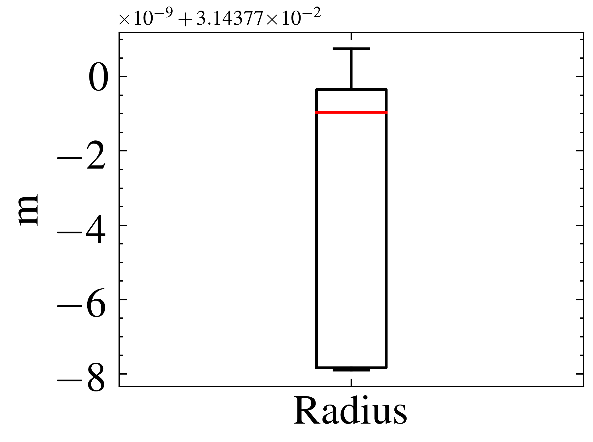
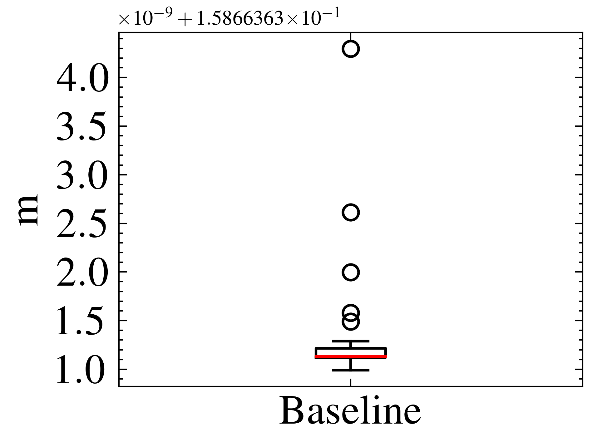
The following section presents and discusses the kinematic parameters obtained via the proposed optimization approach and further compares them to the GT values, taken from the corresponding Universal Robot Description Format (URDF) files. Table I displays the resulting mean values of a total of 100 optimizations with different first initial guesses (FIG) for each parameter of the different kinematic configurations as well as the error with respect to the ground truth values. To obtain the FIG values we sampled from a normal distribution with the mean located at the GT value.

TABLE I: Results of 100 optimizations

Vehicle	GT [m]		Optimization [m]		Error [%]
Vehicle	r	B/L	r	B/L	r	B/L
Turtlebot3	0.033	0.16	0.03144	0.15866	4.73	0.84
Catvehicle	0.03672	2.62	0.38255	2.61462	4.18	0.21

Fig. 8 displays 5 SLSQP optimizations processes for each parameter of the kinematic models, based on the loss functions as defined in (1), and the corresponding boxplots. As illustrated in Fig. 7(a) and 7(c) the curved path segments outweigh the straight path segments in the recorded datasets, this explains the more precise optimization of the baseline (Fig. 8(b)) and wheel base (Fig. 8(f)) of the Turtlebot3 respectively the Catvehicle. Meanwhile, because there are fewer datapoints available in the straight path segments, the wheel radius optimization for the Turtlebot and the Catvehicle converges after 4 iterations (Fig. 8(a)) or 5 iterations (Fig. 8(a)), and the baseline (14 iterations, see Fig. 8(b)) or wheelbase (6 iterations, see Fig. 8(f)) took longer to achieve the desired optimization tolerance of $1e^{-16}$ .

The here proposed pipeline takes less sensor measurements (60 sec on average) compared to other approaches (e.g. 15 min in [23]) to produce reasonably precise estimations of the kinematic parameters. Further the presented method works with an arbitrary trajectory which makes it easier to carry out compared to approaches such as [24] that require a programmed trajectory for calibration. Meanwhile, as can be seen in table II, the optimization problem can be solved fairly fast.

TABLE II: Mean optimization duration of 100 optimizations on AMD Ryzen 7 3700X

Vehicle	Turtlebot		Catvehicle
Vehicle	r	B	r	L
Time [s]	0.0397	0.2206	0.0220	0.8061

VI Conclusion and Future Steps

In this paper, we proposed a novel pipeline for parameter estimation of kinematic models. The pipeline applied minimizes the error of the relative position displacements of an arbitrary landmark compared to the forward kinematics of the vehicle by optimizing the desired parameters using sequential least square optimization. The error, compared to the GT values, of the estimated parameters range between $\approx$ 4.7% with 40s of data and $\approx$ 0.2% with 90s of data.

Since the proposed pipeline heavily depends on the tracking of the observed landmark, occlusions will falsify the results. Therefore, future work will address the fusion of multiple landmarks, to overcome possible occlusions. Further, the development of an online capable pipeline as well as multiple radii estimations, to detect load changes and different abrasions will be tackled in future work.

ACKNOWLEDGMENT

This work was supported by the Austrian Ministry for Climate Action, Environment, Energy, Mobility, Innovation and Technology (BMK) Endowed Professorship for Sustainable Transport Logistics 4.0., IAV France S.A.S.U., IAV GmbH, Austrian Post AG and the UAS Technikum Wien.

References

[1] C. Olaverri-Monreal, “Road safety: Human factors aspects of intelligent vehicle technologies,” in Smart Cities, Green Technologies, and Intelligent Transport Systems. Springer, 2017, pp. 318–332.
[2] R. Siegwart and I. R. Nourbakhsh, Introduction to Autonomous Mobile Robots. USA: Bradford Company, 2004.
[3] S. A. S. Mohamed, M.-H. Haghbayan, T. Westerlund, J. Heikkonen, H. Tenhunen, and J. Plosila, “A survey on odometry for autonomous navigation systems,” IEEE Access, vol. 7, pp. 97 466–97 486, 2019.
[4] Z. Xuexi, L. Guokun, F. Genping, X. Dongliang, and L. Shiliu, “Slam algorithm analysis of mobile robot based on lidar,” in 2019 Chinese Control Conference (CCC), 2019, pp. 4739–4745.
[5] F. Duchoň, J. Hažík, J. Rodina, M. Tölgyessy, M. Dekan, and A. Sojka, “Verification of slam methods implemented in ros,” Journal of Multidisciplinary Engineering Science and Technology (JMEST), 2019.
[6] C. Häne, T. Sattler, and M. Pollefeys, “Obstacle detection for self-driving cars using only monocular cameras and wheel odometry,” in 2015 IEEE/RSJ International Conference on Intelligent Robots and Systems (IROS), 2015, pp. 5101–5108.
[7] J. Jin and W. Chung, “Obstacle Avoidance of Two-Wheel Differential Robots Considering the Uncertainty of Robot Motion on the Basis of Encoder Odometry Information,” Sensors, vol. 19, no. 2, 2019.
[8] W. Ci, Y. Huang, and X. Hu, “Stereo visual odometry based on motion decoupling and special feature screening for navigation of autonomous vehicles,” IEEE Sensors Journal, vol. 19, no. 18, pp. 8047–8056, 2019.
[9] S. Thrun, W. Burgard, and D. Fox, Probabilistic Robotics (Intelligent Robotics and Autonomous Agents). The MIT Press, 2005.
[10] W. Wöber, G. Novotny, L. Mehnen, and C. Olaverri-Monreal, “Autonomous vehicles: Vehicle parameter estimation using variational bayes and kinematics,” Applied Sciences (Switzerland), vol. 10, no. 18, sep 2020.
[11] J. Ko and D. Fox, “Gp-bayesfilters: Bayesian filtering using gaussian process prediction and observation models,” in IROS, 2008.
[12] W. Samek, T. Wiegand, and K.-R. Müller, “Explainable artificial intelligence: Understanding, visualizing, and interpreting deep learning models,” ITU Journal: ICT Discoveries, vol. 1, pp. 49–58, 2018.
[13] W. Samek and K.-R. Müller, Towards Explainable Artificial Intelligence. Springer International Publishing, 2019, pp. 5–22.
[14] G. Montavon, W. Samek, and K.-R. Müller, “Methods for interpreting and understanding deep neural networks,” Digital Signal Processing, vol. 73, pp. 1–15, 2018.
[15] P. Polack, F. Altché, B. d’Andréa Novel, and A. de La Fortelle, “The kinematic bicycle model: A consistent model for planning feasible trajectories for autonomous vehicles?” in 2017 IEEE Intelligent Vehicles Symposium (IV), 2017, pp. 812–818.
[16] K. Lee, C. Jung, and W. Chung, “Accurate calibration of kinematic parameters for two wheel differential mobile robots,” Journal of Mechanical Science and Technology, vol. 25, no. 6, pp. 1603–1611, jun 2011.
[17] R. B. Sousa, M. R. Petry, and A. P. Moreira, “Evolution of odometry calibration methods for ground mobile robots,” in 2020 IEEE International Conference on Autonomous Robot Systems and Competitions, ICARSC 2020. IEEE, apr 2020, pp. 294–299.
[18] G. Antonelli, S. Chiaverini, and G. Fusco, “A calibration method for odometry of mobile robots based on the least-squares technique: theory and experimental validation,” IEEE Transactions on Robotics, vol. 21, no. 5, pp. 994–1004, oct 2005.
[19] J. Borenstein and L. Feng, “UMBmark: a benchmark test for measuring odometry errors in mobile robots,” in Mobile Robots X, W. J. Wolfe and C. H. Kenyon, Eds., vol. 2591, International Society for Optics and Photonics. SPIE, 1995, pp. 113–124. [Online]. Available: https://doi.org/10.1117/12.228968
[20] G. Antonelli and S. Chiaverini, “A Deterministic Filter for Simultaneous Localization and Odometry Calibration of Differential-Drive Mobile Robots,” in Proceedings of the 3rd European Conference on Mobile Robots - ECMR 2007, 2007, pp. 1–6.
[21] B. Naujoks, P. Burger, and H.-J. Wuensche, “Combining deep learning and model-based methods for robust real-time semantic landmark detection,” in 2019 22th International Conference on Information Fusion (FUSION), 2019, pp. 1–8.
[22] D. Kraft et al., “A software package for sequential quadratic programming,” 1988.
[23] F. Galasso, D. L. Rizzini, F. Oleari, and S. Caselli, “Efficient calibration of four wheel industrial agvs,” Robotics and Computer-Integrated Manufacturing, vol. 57, pp. 116–128, 2019.
[24] K. Lee, W. Chung, and K. Yoo, “Kinematic parameter calibration of a car-like mobile robot to improve odometry accuracy,” Mechatronics, vol. 20, no. 5, pp. 582–595, 2010.
[25] L. Cantelli, S. Ligama, G. Muscato, and D. Spina, “Auto-calibration methods of kinematic parameters and magnetometer offset for the localization of a tracked mobile robot,” Robotics, vol. 5, no. 4, 2016.
[26] A. Martinelli, N. Tomatis, A. Tapus, and R. Siegwart, “Simultaneous localization and odometry calibration for mobile robot,” in Proceedings 2003 IEEE/RSJ International Conference on Intelligent Robots and Systems (IROS 2003) (Cat. No.03CH37453), vol. 2, 2003, pp. 1499–1504 vol.2.
[27] R. Kümmerle, G. Grisetti, and W. Burgard, “Simultaneous Parameter Calibration, Localization, and Mapping,” Advanced Robotics, vol. 26, no. 17, pp. 2021–2041, dec 2012.
[28] J. Deray, J. Sola, and J. Andrade-Cetto, “Joint on-manifold self-calibration of odometry model and sensor extrinsics using pre-integration,” in 2019 European Conference on Mobile Robots (ECMR). IEEE, sep 2019, pp. 1–6.
[29] P. Corke, “Robotics, vision and control,” vol. 118, 2017. [Online]. Available: http://link.springer.com/10.1007/978-3-319-54413-7
[30] R. Bhadani, J. Sprinkle, and M. Bunting, “The CAT Vehicle Testbed: A Simulator with Hardware in the Loop for Autonomous Vehicle Applications,” Proceedings of 2nd International Workshop on Safe Control of Autonomous Vehicles (SCAV 2018), Porto, Portugal, 10th April 2018, Electronic Proceedings in Theoretical Computer Science 269, pp. 32–47, 2018.
[31] M. Quigley, K. Conley, B. Gerkey, J. Faust, T. Foote, J. Leibs, R. Wheeler, A. Y. Ng, et al., “Ros: an open-source robot operating system,” in ICRA workshop on open source software, vol. 3, no. 3.2. Kobe, Japan, 2009, p. 5.
[32] R. B. Rusu and S. Cousins, “3d is here: Point cloud library (pcl),” in 2011 IEEE international conference on robotics and automation. IEEE, 2011, pp. 1–4.
[33] N. Koenig and A. Howard, “Design and use paradigms for gazebo, an open-source multi-robot simulator,” in 2004 IEEE/RSJ International Conference on Intelligent Robots and Systems (IROS) (IEEE Cat. No.04CH37566), vol. 3, 2004, pp. 2149–2154 vol.3.
[34] R. Smith et al., “Open dynamics engine,” 2005.
[35] R. Amsters and P. Slaets, “Turtlebot 3 as a robotics education platform,” in Robotics in Education, M. Merdan, W. Lepuschitz, G. Koppensteiner, R. Balogh, and D. Obdržálek, Eds. Cham: Springer International Publishing, 2020, pp. 170–181.
[36] ROBOTIS. Turtlebot 3. https://emanual.robotis.com/docs/en/platform/turtlebot3/overview/. (Accessed on 01/16/2022).