MCRB-based Performance Analysis of
6G Localization under Hardware Impairments
Abstract
Location information is expected to be the key to meeting the needs of communication and context-aware services in 6G systems. User localization is achieved based on delay and/or angle estimation using uplink or downlink pilot signals. However, hardware impairments (HWIs) distort the signals at both the transmitter and receiver sides and thus affect the localization performance. While this impact can be ignored at lower frequencies where HWIs are less severe, modeling and analysis efforts are needed for 6G to evaluate the localization degradation due to HWIs. In this work, we model various types of impairments and conduct a misspecified Cramér-Rao bound analysis to evaluate the HWI-induced performance loss. Simulation results with different types of HWIs show that each HWI leads to a different level of degradation in angle and delay estimation performance.
Index Terms:
Localization, 5G/6G, hardware impairment, CRB, MCRB.I Introduction
Localization will be an indispensable part of future communication systems, both to improve spatial efficiency and optimize resource allocation [1], but also to support high-accuracy context-aware applications such as the tactile internet, augmented reality, and smart cities [2, 3]. By taking advantage of a large array dimension and wide bandwidth of high-frequency (e.g., mmWave and sub-THz) communication systems, high angular and delay resolution, and hence accurate position estimation can be achieved [4]. Most localization algorithms rely on accurate models of the received signals as a function of the channel parameters (angles, delays, Dopplers) of the propagation environment. The presence of hardware impairments such as phase noise, carrier frequency offset, mutual coupling, power amplifier nonlinearity, in-phase and quadrature imbalance, distort the pilot signals. As a result, when algorithms derived from a mismatched model (i.e., without or with limited information about the hardware impairments), the localization performance is unavoidably affected.
There has been extensive research on the effect of hardware impairments in communication systems in terms of spectral efficiency analysis [5], beamforming optimization [6], and channel estimation [7, 8]. The research on localization and sensing considering HWIs is also catching up. The effect of PN on automotive radar [9, 10, 11], mutual coupling on DOA estimation [12], IQI on mmWave localization [13], and PAN on joint radar-communication (JRC) systems [14] are discussed. In [15], the impairments are jointly modeled using a HWI factor. Nevertheless, this factor is not able to capture the contribution of each individual HWI. Hence, critical questions, such as how much error will be caused by a mismatched model, and how much HWI we can tolerate for 5G/6G localization, remain unanswered.
In this work, we consider an orthogonal frequency-division multiplexing-based localization system with hardware impairments. The corresponding localization algorithm may or may not have knowledge about these hardware impairments, where in the latter case the localization algorithm operates under model mismatch, as it does not know the PAN and the residual impairments of PN, CFO, and MC. We use the Cramér-Rao bound to predict the performance in angle, delay, and position estimation under the different models, and employ the misspecified Cramér-Rao bound [16, 17, 18] to quantify the estimation performance loss due to model mismatch. The results show that different types of impairments affect angle and delay estimation in different ways.
II System Model
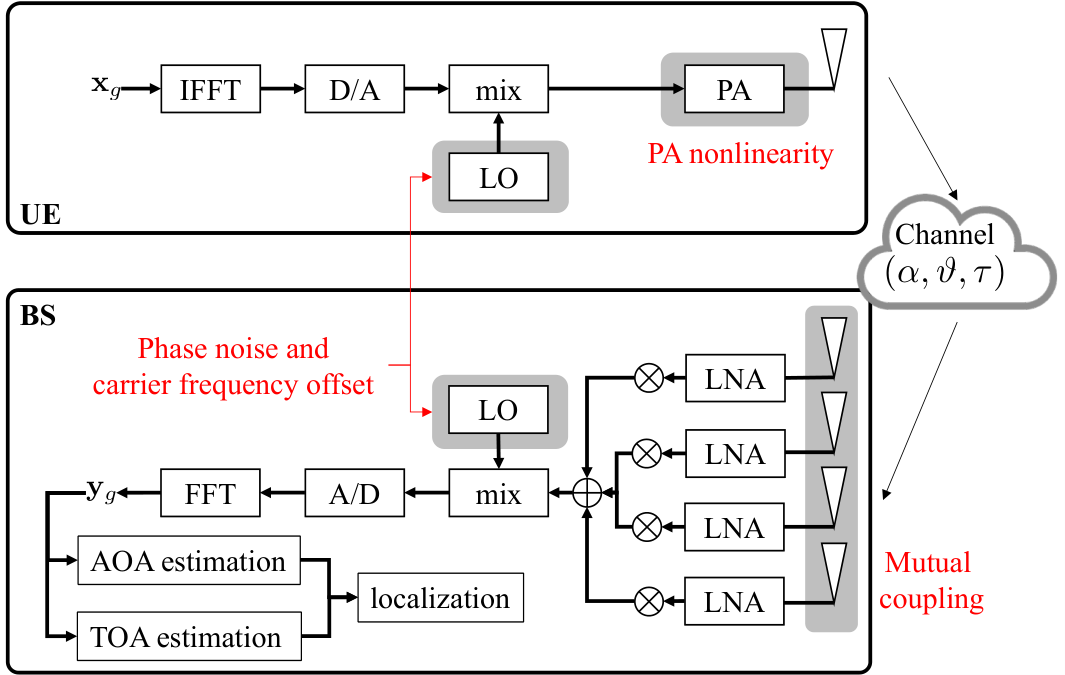
In this section, we start with the hardware impairment-free model and then describe the hardware impairment model, as shown in Fig. 1. We consider a simplified uplink scenario with a line-of-sight channel between a base station equipped with an -antenna uniform linear array and a synchronized single-antenna user equipment, both with a single radio-frequency chain. The assumptions of single-antenna user equipment, perfect synchronization, and pure line-of-sight may not be realistic in practice, but are an initial step to analyze and understand hardware impairments. We set the center of the BS array as the origin of the global coordinate system. The relation between the angle-of-arrival , the delay , and the UE position can be expressed as , where is the speed of light.
II-A Hardware Impairment-free Model
Considering the transmitted orthogonal frequency-division multiplexing symbol at -th transmission () and -th subcarrier (), , its observation at the base station can be formulated as
| (1) |
where is the combiner at the BS for the -th transmission; is the channel vector at the th subcarrier with a complex gain (amplitude and phase ) as , an receiver steering vector , and a delay component ( is the subcarrier spacing). We assume remains the same during transmissions (within the coherence time). Finally, is the noise following a complex normal distribution, with , where is the noise power spectral density (PSD) and is the total bandwidth. The average transmission power , where is the load impedance. By concatenating all the received symbols into a column, we obtain the received symbol block as , where can be expressed as
| (2) |
in which , , and denotes the Hadamard product.
II-B Hardware Impairments
The considered HWIs are highlighted in gray in Fig. 1 [19]. We select residual PN, residual CFO, residual MC, and PAN. The in-phase and quadrature imbalance and imperfections of analog to digital converter, digital to analog converter, low-noise amplifier (LNA) and mixer are left for future work. By focusing on residual PN, CFO, and MC, our analysis can impose requirements on the corresponding PN, CFO, and MC estimation accuracy.
II-B1 Phase Noise and Carrier Frequency Offset
Imperfect local oscillators in the up-conversion and down-conversion processes add PN to the carrier wave phase. In addition, when the down-converting local oscillator in the receiver does not perfectly synchronize with the received signal’s carrier [20], CFO occurs. Generally, both PN and CFO are tackled by the receiver [21], so we only consider the residual PN and residual CFO at the receiver. With PN and CFO, the observation, , is modified as [22]
| (3) |
where is without PN or CFO (i.e., from (1)), is the FFT matrix,
| (4) |
is the residual11 1 Since represents residual PN that remains after PN mitigation processing (e.g., [23, 24]), it is assumed to be independent across time. phase noise matrix with , and accounts for the CFO. In (3), the vector is converted to the time domain by , where the successive phase noise samples, as well as the CFO are applied. Finally, extracts the -th subcarrier after applying an FFT to . The CFO matrix considers both inter-OFDM symbol phase changes as well as inter-carrier interference [22, 25]:
| (5) |
where , in which is the length of the cyclic prefix, and is the normalized residual CFO with .
II-B2 Mutual Coupling
Mutual coupling refers to the electromagnetic interaction between the antenna elements in an array [12]. Similar to PN and CFO modeling, we consider residual mutual coupling, which remains after a calibration procedure. For a uniform linear array, we introduce the banded mutual coupling matrix at the Rx. Here, is the MC matrix with as the MC coefficient, and represents the uncalibrated MC matrix that is modeled as random (residual MC matrix) with each element . The MC leads to the substitution [12]
| (6) |
II-B3 Power Amplifier Nonlinearity
For the PA nonlinearity, we consider a -th order memoryless polynomial nonlinear model with a clipping point as [19]
| (7) |
where denotes the transmitted signals in time domain and are complex-valued parameters. Note that the PA affects the time domain signals and we assume no digital pre-distortion is implemented. We also use non-oversampled signals as the input of the PA for tractable localization performance analysis.
II-C Hardware Impaired Model
Considering the hardware impairments of PN, CFO, MC, and PA nonlinearity and substituting (3), (6), and (7) into (2), the observation can be rewritten in the frequency domain as
| (8) | ||||
where overloads the notation for the PA, and operates point-wise on each of the elements in the time-domain sequence. The FFT and IFFT matrices switch between time and frequency domain representations in order to apply the PN, CFO and PA in the correct (time) domain, while providing a frequency domain representation. We use to denote the noise-free observation. Note that the PA model in (7) does not consider the out-of-band emissions, but only the in-band distortion.
Finally, we consider a model without the PAN and the residual noise of PN, CFO, and MC:
| (9) | ||||
where is the noise-free version of the observation.
II-D Summary of the Models
To summarize, we have defined three types of signal models as follows.
- •
M0: The model defined in (1) without considering the hardware impairment.
- •
M1: The model that considers knowledge of the various hardware impairments defined in (8).
- •
M2: With the practical assumption that not all the hardware impairments information is available, we use the model defined in (9).
In the rest of the work, M0 will not be discussed, and the models M1 and M2 will be used for CRB analysis, as well as for localization performance evaluation.
III Localization Algorithm
The maximum likelihood estimation is employed when the observation is generated from the same model used by the algorithm. On the other hand, the mismatched maximum likelihood estimation is used when the observation is generated from a different model than what is used by the algorithm. In the latter case, we will denote the generative model by true model, while the model used by the estimator is called the mismatched model.
III-A MLE
If , the maximum likelihood estimation of the UE position and channel gain is
| (10) |
where is the log-likelihood of the true model. Since appears linearly in the noise-free observation, we can use a plug-in estimate, and solve for the position by a coarse grid search to find an initial estimate , followed by a backtracking line search [26]. For instance, when ,
| (11) |
III-B MMLE
If , but the estimator uses , the mismatched maximum likelihood estimation is given by
| (12) |
For instance, when and ,
| (13) |
IV Lower Bounds Analysis
In the next, we derive the CRB for M222 2 The CRB of M1 can be obtained similarly, which will not be detailed in this work., as well as the misspecified Cramér-Rao bound for the mismatched estimator in (13) with and .
IV-A CRB Analysis
We define a channel parameter vector as and a state vector . Given the signal model in (9) and , the CRB of the mismatched model can be obtained as [27]
| (14) |
where
| (15) | ||||
| (16) |
Here, , are the Fisher information matrices (FIMs) of the channel parameter vector and UE state vector, is getting the real part of a complex number, and is the Jacobian matrix using a denominator-layout notation with and . Based on the FIM, we further define the angle error bound (AEB), delay error bound (DEB) and position error bound (PEB) as
| (17) | ||||
| (18) | ||||
| (19) |
where returns the trace of a matrix, and is getting the element in the th row, th column of a matrix. The bounds from (17)–(19) will be used to evaluate the localization performance.
IV-B Misspecified CRB
The model is said to be mismatched or misspecified when , while the estimation is based on the assumption that ), where . Due to the one-to-one mapping between and , we can also write and . The lower bound of using a mismatched estimator can be obtained as [18]
| (20) |
where is the true channel parameter vector, is the pseudo-true parameter vector (which will be introduced soon), and are two possible generalizations of the FIMs. The LB is a bound in the sense that (typo ‘’ is corrected as ‘’)
| (21) |
where the expectation is with respect to . What remains is the formal definition and computation of the pseudo-true parameter and .
IV-B1 Pseudo-true Parameter
Assume the probability density function of the true model, where the observation data come from, is , where is the received signals and (4 unknowns for this 2D case) is the vector containing all the channel parameters. Similarly, the probability density function of the mismatched model for the received signal can be noted as . The pseudo-true parameter vector is defined as the point that minimizes the Kullback-Leibler divergence between and as
| (22) |
We define , and the pseudo-true parameter can be obtained as (details can be found in Appendix A)
| (23) |
Hence, can be found by solving (13) with the observation , which can be accomplished using the same algorithm in Sec. III, initialized with the true value .
IV-B2 MCRB Component Matrices
The matrices and can be obtained based on the pseudo-true parameter vector as
| (24) |
and
| (25) |
where the calculation of each element inside the matrices and can be found in Appendix B.
V Numerical Results
V-A Default Parameters
We consider a 2D uplink scenario with a single-antenna UE and a BS with a 20-element ULA. The pilot signal is chosen with a constant average energy and random phase. The simulation parameters33 3 The PA parameters are estimated from the measurements of the RF WebLab, which can be remotely accessed at www.dpdcompetition.com. can be found in Table I.
| Parameters | True Model | Mismatched Model |
|---|---|---|
| BS Antennas | ||
| UE Antennas | ||
| RFC at BS/UE | ||
| Carrier Frequency | ||
| Bandwidth | ||
| Transmissions | ||
| Subcarriers | ||
| Length of the CP | ||
| Load Impedance | ||
| Noise PSD | ||
| Noise Figure | ||
| PN (residue) | ||
| CFO (residue) | (0.71 ppm) | |
| MC (matrix) | +, - | |
| MC (residue) | ||
| PA Parameters | +, - | |
| + | ||
| PA Clipping Voltage | ||
V-B Estimation Results vs. Bounds
We first evaluate the position estimation performance of the two estimators (MLE (11) and MMLE (13), where observations come from the hardware-impaired model M1). The simulation results are compared with three different lower bounds, namely, LB (the lower bound of using the M2 to process the data from the M1), CRB-M1, and CRB-M2. Note that the average transmission power is calculated without considering the nonlinearity of the power amplifier (calculated before the PA). Fig. 2 shows the positioning errors obtained by the estimators, along with the corresponding theoretical bounds, with respect to . From the figure, we can see that at low transmit powers, the LB and CRBs coincide, implying that the HWIs are not the main source of error. At higher transmit powers (after 20 dBm), LB deviates from the CRBs and the positioning performance is thus more severely affected by HWIs. The MMLE closely follows the LB, indicating the validity of the LB. In terms of CRB-M1, we observe the bound converges to a certain value after 30 dBm, due to the PAN, while the CRB-M2 keeps a fixed downward trend.
(a) PN ()
(b) CFO ()
(c) MC ()
(d) PAN ()
V-C The Effect of Individual Impairments
To gain a deeper understanding, we study the impact of hardware impairments on angle and delay estimation, considering different hardware impairments separately. The results are shown in Fig. 3 for (a) PN, (b) CFO, (c) MC, and (d) PAN. Multiple realizations (multiple hardware realizations with a fixed pilot signal for (a)-(c) and multiple pilot signal realizations for (d)) are performed for each type of the HWI. We can see that different types of the hardware impairments affect angle and delay estimation differently. The PN and PAN affect both angle and delay estimation, however, the effect of PAN is mainly caused by the distortion of the pilot signals, whereas the effect of PN depends on the residual noise level . The CFO and MC have a more significant effect on angle estimation compared to delay estimation since the CFO affects the phase changes across beams and the MC distorts the steering vector. In addition, within reasonable levels of hardware impairments, the CRBs with perfect knowledge of the impairments (CRB-M1) are close to the CRBs of the mismatched model (CRB-M2).
In Fig. 4, we evaluate the localization performance (which in turn depends on the AEB (in terms of degree) and DEB (in terms of meter) shown in Fig. 3) as a function of the standard deviation of PN (similar patterns can be seen for CFO and MC) for various values of average transmission power using 100 realizations of PN. The impairments produce a larger perturbation in the high SNR scenario. As for low SNR, the noise level is high enough and the impairments, under a certain level, will not degrade the PEB too much.
VI Conclusion
hardware impairments present a crucial roadblock to achieving high performance in radio-based localization. We modeled different types of hardware impairments and utilize the misspecified Cramér-Rao bound to evaluate the error caused by model-mismatch. The effects of residual PN, residual CFO, residual MC and PAN on angle/delay estimation are evaluated. We found that PN and PAN affect both angle and delay estimation, whereas CFO and MC have a more significant effect on angle estimation. We also observed that with perfect knowledge of the hardware impairments, the bound is close to the bound of the mismatched model, but will saturate at a certain level in the high SNR regime due to the PAN. In conclusion, dedicated pilot signal design, HWIs estimation and mitigation algorithms are needed for accurate localization in 6G systems.
Acknowledgment
This work was supported, in part, by the European Commission through the H2020 project Hexa-X (Grant Agreement no. 101015956) and by the MSCA-IF grant 888913 (OTFS-RADCOM).
Appendix A
The pseudo-true parameters can be calculated as
After some manipulation, we find that
For each received symbol at the th transmission and th subcarrier, , by ignoring the indices and we can have
from which (23) follows immediately.
Appendix B
To obtain matrices and , we need to calculate the derivative of the noise-free version of the mismatched model with respect to the channel parameters inside the vector .
B-A First-order Derivatives
For the first-order derivative parts of the matrix , note that is dependent of and , is dependent of angle-of-arrival , is dependent of delay . We can write , , , . where , , and
B-B Second-order Derivatives
The second-order derivative parts of the matrix in equation (25) can be obtained based on the dependence of the channel components () and unknowns () with several examples as , , , , and . where , , , , and .
References
- [1] R. Di Taranto et al., “Location-aware communications for 5G networks: How location information can improve scalability, latency, and robustness of 5G,” IEEE Signal Process. Mag., vol. 31, no. 6, pp. 102–112, Oct. 2014.
- [2] G. Kwon et al., “Joint communication and localization in millimeter wave networks,” IEEE J. Sel. Topics Signal Process., Sep. 2021.
- [3] Z. Xiao et al., “An overview on integrated localization and communication towards 6G,” Sci. China Inf. Sciences, vol. 65, no. 3, pp. 1–46, Mar. 2022.
- [4] H. Chen et al., “A tutorial on terahertz-band localization for 6G communication systems,” arXiv preprint arXiv:2110.08581, Oct. 2021.
- [5] O. Kolawole et al., “Impact of hardware impairments on mmwave MIMO systems with hybrid precoding,” in IEEE Wireless Commun. Netw. Conf., Apr. 2018.
- [6] H. Shen et al., “Beamforming optimization for IRS-aided communications with transceiver hardware impairments,” IEEE Trans. Commun., vol. 69, no. 2, pp. 1214–1227, Oct. 2020.
- [7] Y. Wu et al., “Efficient channel estimation for mmwave MIMO with transceiver hardware impairments,” IEEE Trans. Veh. Technol., vol. 68, no. 10, pp. 9883–9895, Aug. 2019.
- [8] N. Ginige et al., “Untrained DNN for channel estimation of RIS-assisted multi-user OFDM system with hardware impairments,” in IEEE 32nd Annu. Int. Symp. Pers. Indoor Mobile Radio Commun., Sep. 2021, pp. 561–566.
- [9] H. C. Yildirim et al., “Impact of phase noise on mutual interference of FMCW and PMCW automotive radars,” in 16th Eur. Radar Conf. IEEE, Oct. 2019, pp. 181–184.
- [10] M. Gerstmair et al., “On the safe road toward autonomous driving: Phase noise monitoring in radar sensors for functional safety compliance,” IEEE Signal Process. Mag., vol. 36, no. 5, pp. 60–70, Sep. 2019.
- [11] K. Siddiq et al., “Phase noise in FMCW radar systems,” IEEE Trans. Aerosp. Electron. Syst., vol. 55, no. 1, pp. 70–81, Feb 2019.
- [12] Z. Ye et al., “DOA estimation for uniform linear array with mutual coupling,” IEEE Trans. Aerosp. Electron. Syst., vol. 45, no. 1, pp. 280–288, Mar. 2009.
- [13] F. Ghaseminajm et al., “Localization error bounds for 5G mmWave systems under I/Q imbalance,” IEEE Trans. Veh. Technol., vol. 69, no. 7, pp. 7971–7975, Apr. 2020.
- [14] F. Bozorgi et al., “RF front-end challenges for joint communication and radar sensing,” in 1st IEEE Int. Online Symp. Joint Commun. Sens., Feb. 2021.
- [15] F. Ghaseminajm et al., “Localization error bounds for 5G mmWave systems under hardware impairments,” in IEEE 32nd Annu. Int. Symp. Pers. Indoor Mobile Radio Commun., Sep. 2021, pp. 1228–1233.
- [16] C. D. Richmond et al., “Parameter bounds on estimation accuracy under model misspecification,” IEEE Trans. Signal Process., vol. 63, no. 9, pp. 2263–2278, Mar. 2015.
- [17] F. Roemer, “Misspecified Cramér-Rao bound for delay estimation with a mismatched waveform: A case study,” in IEEE Int. Conf. Acoust., Speech Signal Process., May. 2020, pp. 5994–5998.
- [18] S. Fortunati et al., “Performance bounds for parameter estimation under misspecified models: Fundamental findings and applications,” IEEE Signal Process. Mag., vol. 34, no. 6, pp. 142–157, Nov. 2017.
- [19] T. Schenk, RF imperfections in high-rate wireless systems: Impact and digital compensation. Springer Science & Business Media, 2008.
- [20] A. Mohammadian et al., “RF impairments in wireless transceivers: Phase noise, CFO, and IQ imbalance–A survey,” IEEE Access, vol. 9, pp. 111 718–111 791, Aug. 2021.
- [21] N. Hajiabdolrahim et al., “An extended Kalman filter framework for joint phase noise, CFO and sampling time error estimation,” in 31st Annu. Int. Symp. Pers. Indoor Mobile Radio Commun. IEEE, 2020.
- [22] D. D. Lin et al., “Joint estimation of channel response, frequency offset, and phase noise in OFDM,” IEEE Trans. Signal Process., vol. 54, no. 9, pp. 3542–3554, Aug. 2006.
- [23] O. H. Salim et al., “Channel, phase noise, and frequency offset in OFDM systems: Joint estimation, data detection, and hybrid cramér-rao lower bound,” IEEE Trans. Commun., vol. 62, no. 9, pp. 3311–3325, Jul. 2014.
- [24] M. Chung et al., “Phase-noise compensation for OFDM systems exploiting coherence bandwidth: Modeling, algorithms, and analysis,” IEEE Trans. Wireless Commun., Oct. 2021.
- [25] T. Roman et al., “Blind frequency synchronization in OFDM via diagonality criterion,” IEEE Trans. Signal Process., vol. 54, no. 8, pp. 3125–3135, Jul. 2006.
- [26] J. Nocedal et al., Numerical optimization. Springer Science & Business Media, 2006.
- [27] A. Elzanaty et al., “Reconfigurable intelligent surfaces for localization: Position and orientation error bounds,” IEEE Trans. Signal Process., vol. 69, pp. 5386–5402, Aug. 2021.