Evaluation of radiative depolarization in the future Circular Electron-Positron ColliderPreprint: APS/123-QED
Abstract
Polarized lepton beams are an important aspect in the design of the future 100 -scale Circular Electron-Positron Collider (CEPC). Precision beam energy calibration using resonant depolarization, as well as longitudinally polarized colliding beams are being actively investigated. The achievable beam polarization level for various beam energies and application scenarios depends on the radiative depolarization in the collider rings. In this paper the radiative depolarization effects are evaluated for a CEPC collider ring lattice with detailed machine imperfections and corrections. Simulations with the SLIM and Monte-Carlo approaches using the Bmad/PTC codes are compared with the theory of the effects of spin diffusion for ultra-high beam energies and the validity of the theories is thereby addressed. The paper concludes with a summary and suggestions for further investigations.
I Introduction
After the discovery of the Higgs particle at the Large Hadron Collider (LHC), a study of the Circular Electron Positron Collider (CEPC) was launched as one of the global design efforts of future electron-positron circular colliders Abada et al. 2019; Shiltsev and Zimmermann 2021, for precision measurements of Higgs boson properties and electroweak interactions, as well as direct searches for new physics with an unprecedented accuracy. In the Conceptual Design Report (CDR) The CEPC Study Group 2018 released in November 2018, the CEPC was designed as a double-ring collider with a circumference of about 100 , and to be operated at beam energies of around 45 as a Z factory, 80 as a W factory and 120 as a Higgs factory. After the CDR, the CEPC accelerator entered the phase of the Technical Design Report (TDR) endorsed by the CEPC International Advisory Committee (IAC). Recent updates of the CEPC accelerator R&D are summarized in CEPC Accelerator Study Group 2022.
Beam polarization is an important design aspect of the CEPC. On one hand, the resonant depolarization technology (RD) Derbenev et al. 1980 is essential for precision beam energy calibration at the Z-pole and the WW threshold. RD utilizes a horizontal oscillating magnetic field to excite a vertically polarized beam. As the excitation frequency is scanned, the beam gets depolarized when the perturbation is resonant with the spin precession frequency, which is closely related to the beam energy. RD requires a vertical beam polarization level of 5%10% at the CEPC, according to experience at LEP Assmann et al. 1998. On the other hand, colliding beam experiments with longitudinal beam polarization, which would greatly broaden the potential of the physics program, are also being explored at the CEPC Duan et al. 2019. For this purpose, a longitudinal beam polarization of at least 50% for one or both and beams at the interaction points is desired. These require preparation and maintenance and then manipulation of the polarized beams with spin rotators.
Spin rotators have been successfully implemented into the CEPC CDR lattice for the Z-pole energy in a separate study Xia et al. 2022. Note that since the and beams in the CEPC are in separate rings, their spin helicities can be controlled independently.
The precession of the spin expectation value , and of , of a relativistic charged particle, in electric and magnetic fields follows the Thomas-BMT equation L H Thomas 1964; Bargmann et al. 1959, which, for a circular accelerator or storage ring, can be expressed in the following form,
| (1) |
with
| (2) |
where is the spin-precession vector on the closed orbit at the azimuthal angle . and denote the contribution of the fields on the design orbit and the magnet errors/correction fields to the spin precession vector, respectively. is due to the orbital oscillations relative to the closed orbit. We use a Frenet-Serret coordinate system, where are the unit vectors pointing radially outwards, vertically upwards and longitudinally (clockwise), respectively, so that they form a right-handed unit-vector basis. In this coordinate system, the particle’s phase-space coordinate can be expressed as . and are the transverse coordinates of the particle. The transverse phase-space momenta and are normalized by the reference momentum , namely and , respectively. where is the time difference between the particle and the reference particle arriving at the azimuthal angle . , where and are the velocity of the particle and light, respectively. is the relative energy deviation. The spin polarization of an electron bunch is the ensemble average of the .
In a circular accelerator running at a fixed energy is a periodic function of , for which there is a unit-length periodic solution of Eq. (1), , satisfying . Then a spin vector perpendicular to precesses by a rotation angle in one revolution around , where is called the closed-orbit spin tune. In a storage ring designed with a planar geometry and no solenoids (hereafter referred as the “planar ring”), is close to the vertical direction, and , where for electrons (positrons), and is the relativistic factor for the design energy.
These key concepts of the spin motion on the closed orbit can be extended to the more general phase-space coordinates. One special unit-length solution of Eq. (1) is the invariant spin field (ISF) Barber et al. 2004, , satisfying the periodicity condition and satisfying Eq. (1) along particle trajectories, , obeying Hamilton’s equations. Assuming that the orbital motion is integrable, so that the orbital motion can be expressed in terms of action-angle variables, the analogue of for the combined betatron and synchrotron motion with orbital actions , is the amplitude-dependent spin tune describing the rate of spin precession around Barber et al. 2004. The projection of the spin vector of a particle on the invariant spin field is an adiabatic invariant of its spin motion Hoffstaetter et al. 2006. On the closed orbit, and reduce to and , respectively, but for typical orbital amplitudes with electrons in any case.
Machine imperfections and orbital oscillations contribute to and respectively, and may perturb the spin motion in a resonant manner when the following condition of spin-orbit coupling resonances (spin resonances in short) is nearly satisfied,
| (3) |
where and are the horizontal, vertical betatron tunes and the synchrotron tune, respectively. deviates from significantly near these spin resonances. As will be seen below, in perturbative estimates of spin motion, is replaced by in the above resonance condition. Note that the orbital tunes and in the above definition of the spin resonances, are conventionally used in the case of weak couplings, reduced from the more general orbital tunes , and obtained from the orbital eigen-analysis Chao 1979. Spin resonances with , are called integer spin resonances. In a perfectly aligned planar ring with no solenoids is vertical. In a misaligned ring can deviate strongly from the design direction when is near an integer. Spin resonances with and are called first-order spin resonances and higher-order spin resonances, respectively.
Unlike polarized proton beams which must be polarised at the source, beams can also become spontaneously polarized in a storage ring by the emission of synchrotron radiation. In a perfectly aligned ring with no solenoids with vertical the polarization is vertical but in general the polarization of the beam is along . The evolution of the beam polarization in an electron storage ring for an initially unpolarised beam is
| (4) |
where
| (5) |
where is a unit vector along the particle’s direction of motion, and , is the direction of the guiding magnetic field, which is normally vertical. is the equilibrium beam polarization taking into account the orbital imperfections, but disregarding the radiative depolarization effect Baier et al. 1970. The time constant of the Sokolov-Ternov effect, , is
| (6) |
In an ideal planar ring, is 92.4%. In contrast, as mentioned, for an imperfect storage ring near integer values of , may deviate from the vertical direction, and lead to a reduced level of .
In addition to the Sokolov-Ternov effect, synchrotron radiation also causes radiative depolarization in electron storage rings, namely the spin diffusion effect. It is implicit in standard literature Derbenev and Kondratenko 1973; Mane 1987 that the polarization at each point in phase space is parallel to . This is the the so-called ISF approximation which we discuss again in the Conclusions. A photon emission perturbs the orbital motion and leads to a change in and thus a slightly different . The stochastic nature of synchrotron radiation, then leads to a diffusion in and thus a reduction of beam polarization Baier and Orlov 1966, which has also been called “non-resonant spin diffusion” Derbenev et al. 1979. However, in the proximity of spin resonances where spin motion becomes far from adiabatic, is no longer an invariant of motion, and it has been suggested that the above physics picture is no longer complete. Then a second mechanism, which could be important at very high energy, namely the repetitive fast but “uncorrelated” crossing of the spin resonances, due to stochastic photon emissions, would be another source of radiative depolarization Kondratenko 1974; Derbenev and Kondratenko 1975, which has also been called “resonant spin diffusion” Derbenev et al. 1979. In any case, the evolution of beam polarization in an electron storage ring is a compromise between the spontaneous polarization build-up and the radiative depolarization effects.
Analytical estimates of the equilibrium beam polarization in the presence of just non-resonant spin diffusionare generally made with the Derbenev-Kondratenko (DK) formula Derbenev and Kondratenko 1973; Mane 1987:
| (7) |
where the brackets denote an average over the orbital phase space at azimuth . The spin-orbit coupling function quantifies the depolarization. This can be rather large near spin resonances, leading to a reduced level of equilibrium polarization, as well as a smaller self-polarization build-up time relative to
| (8) |
where is the time constant of the spin diffusion effect,
| (9) |
The key to evaluation of the DK formula lies in the evaluation of . As already indicated, in the derivation of the DK formula, only the first mechanism (non-resonant spin diffusion) of radiative depolarization was included. Then as suggested in Derbenev and Kondratenko 1975; Derbenev et al. 1979, the DK formula should be augmented to take into account the effects of resonant spin diffusion too.
In a mainly-planar storage ring, the equilibrium polarization can also be approximated by
| (10) |
This equation disregards the tiny effect of kinetic polarization associated with the term in Eq. 7, but captures the essentials of the trade-off between the Sokolov-Ternov effect and the radiative depolarization effect, regardless of the underlying mechanism of radiative depolarization. The strength of the depolarization effects is quantified by the ratio .
So far, the evaluation of the equilibrium polarization in real storage rings has involved two classes of computer algorithms, as reviewed in detail in Ref D. P. Barber, G. Ripken a; D. P. Barber, G. Ripken b. One class of algorithms numerically evaluates and and then applies Eq. (7) to calculate the equilibrium polarization. For example, SLIM Chao 1981 treats linearized orbital and spin motion, and thus reflects the influence of first-order spin resonances while taking into account the effects of tilted near integer values of . It can be classed as a first-order perturbative algorithm. Several other algorithms employ full three-dimensional spin motion S. R. Mane 1987; Yokoya 1992; K. Yokoya 1999; Yokoya 1987 and thus expose the higher-order spin resonances resulting from that. Among these are the higher-order perturbative algorithm of Ref. S. R. Mane 1987 and the non-perturbative approaches of the SODOM algorithms Yokoya 1992; K. Yokoya 1999.
The other class of algorithms evaluate the depolarization time through Monte-Carlo simulations, like SITROS Kewisch 1985, SLICKTRACK Barber 2005 and Bmad Sagan et al., and then calculate the equilibrium polarization with Eqs. (5), (6) and (10). Unlike the previous class of algorithms, the Monte-Carlo method, with its use of full three-dimensional spin motion, exposes both first-order and higher-order spin resonances automatically, while not relying on the calculation of and and Eq. (7). Nor is it dependent on other theories of spin diffusion. Therefore, the Monte-Carlo method can be used to check theoretical models of radiative depolarization. The Monte-Carlo method has the additional advantage that it can handle non-linear orbital motion such as that caused by beam-beam forces.
Resonant and non-resonant spin diffusion for ultra-high energy electron storage rings have been discussed in detail by Derbenev, Kondratenko and Skrinsky Derbenev et al. 1979. These theories were later compared with the experiments with vertically polarized beams in LEP Assmann et al. 2001. In the past decade, global interest has arisen in building future circular colliders. Mane worked out a scaling of equilibrium beam polarization at ultra-high beam energies and studied possibilities for using Siberian snakes to mitigate the depolarization while retaining self-polarization at the same time Mane 2014. Nikitin evaluated the radiative depolarization and the equilibrium transverse polarization in these super electron-positron circular colliders theoretically, and discussed options of achieving longitudinally polarized colliding beams Nikitin 2019; S. A. Nikitin 2020. There are also attempts to re-evaluate the radiative depolarization and equilibrium beam polarization using an approach based on the Bloch equation Heinemann et al. 2019; Beznosov Oleksii 2020; K. Heinemann and others 2020.
There have already been some simulations for the equilibrium polarization for the future circular colliders at ultra-high energies. For example, Gianfelice-Wendt launched Monte-Carlo simulations with the SITROS packageKewisch 1985 of the achievable self-polarization at CERN’s Future Circular collider (FCC-ee) E Gianfelice-Wendt 2016 at 45 and 80 beam energies, aiming at energy calibration using RD. Quadrupole misalignments and beam-position-monitor errors were introduced in a simplified ring lattice without the interaction regions. It was shown that a reasonable polarization level can be achieved in the collider ring at both energies with a well planned orbit correction scheme, while asymmetric wigglers are necessary to boost the self-polarization build-up at 45 . Koop developed a Monte-Carlo simulation code with a simplified model including one-turn energy-dependent spin precession and a lumped element to model spin perturbations, in addition to synchrotron oscillations and synchrotron radiation. This simulation code was also used to study the RD process Koop 2018.
On our side a Monte-Carlo simulation of radiative depolarization based on the Polymorphic Tracking Code (PTC) Forest et al. 2002; Forest was developed in Ref. Duan et al. 2015. The equilibrium beam polarization was simulated for a model ring lattice with a circumference of 50 and artificial skew quadrupoles to excite betatron spin resonances. That study supported the suggestion in Ref. Derbenev et al. 1979 that the spin dynamics enter an “uncorrelated regime” of spin resonance crossing at ultra-high beam energies. However, it was not clear if this paradigm shift would exist in a realistic imperfect ring.
For this paper, we extend our studies to the radiative depolarization effects for the CEPC at the Z pole as well as higher beam energies, and for various operation scenarios. We use a CEPC CDR lattice that contains two interaction regions, and includes detailed error modeling and corrections. This lattice does not contain solenoids and has relatively weak orbital correctors with horizontal magnetic fields, and belongs to the category of the “planar ring”. We present the theories of radiative depolarization applicable to this case. Monte-Carlo simulations based on the PTC code Forest et al. 2002; Forest; Duan et al. 2015 were then applied to estimate the radiative depolarization effects, which are compared to those from the theories of radiative depolarization at ultra-high beam energies.
This paper is arranged as follows. More details of theories of radiative depolarization in ultra-high energy electron storage rings are reviewed in Section II. The setup of the CEPC lattice is introduced in Section III. In Section IV, the theories are applied to the CEPC lattice to evaluate the depolarization effects. Section V, presents the results of Monte-Carlo simulations for the equilibrium polarization for the standard CEPC lattice as well as for a lattice with asymmetric wigglers and a double RF system and these are compared with the results from theoretical models. The last section provides a summary and suggestions for future numerical and theoretical work.
II Theories of radiative depolarization
In the following we focus our analysis on realistic planar electron storage rings. Severe depolarization may occur when the closed-orbit spin tune is near an integer , so that is tilted from the design direction and then as shown below, the two first-order “parent” synchrotron spin resonances can therefore be strong, even overlapping with each other. Depolarization also occurs near first-order “parent” betatron spin resonances . Moreover, even if is not near an integer, its distance to adjacent integer spin resonances and first-order spin resonances is less than 220 . As the spread of the spin precession frequency increases with the beam energy, it becomes more difficult to attain high polarization. In particular, as we show in the perturbation theory sketched below, higher-order synchrotron “sideband” spin resonances , where is an integer and , become much more prominent, compared to those in lower-energy electron storage rings. The strongest of these resonances are centered on first-order “parent” spin resonances. Note that in this context an integer spin resonance will be a “sideband” spin resonance of the “parent” first-order synchrotron spin resonances . Note also that this kind of resonance can even occur when the ring is perfectly aligned and is not tilted from the design direction as, for example, when spin rotators make horizontal in a region with quadrupoles and dispersion. The higher-order “parent” resonances also carry synchrotron sideband resonances.
Observations of beam polarization in electron storage rings have so far been in broad agreement with the expectations of Eq. (7), taking into account of the depolarization associated with these first-order and higher-order spin resonances. However, as already mentioned and as proposed in Ref. Kondratenko 1974; Derbenev and Kondratenko 1975; Derbenev et al. 1979, the above picture with its consequences explored using perturbation theory, belongs to the “non-resonant spin diffusion”, while a somehow different picture of “resonant spin diffusion” is required for ultra-high beam energies. This argument is better appreciated from a “dynamical” perspective as described in more detail below. Under certain circumstances, the combined influence of synchrotron oscillation and synchrotron radiation could lead to “repetitive fast but uncorrelated crossings” of the underlying spin resonances. Note that in this case, the influence of the resonant spin diffusion is not limited to the close proximity of the underlying spin resonances.
Now, to set the scene, we’ll first present the depolarization theory of the “parent” first-order spin resonances, or “first-order theory” in short. We explicitly derive the dominating contribution of first-order “parent” synchrotron spin resonances to radiative depolarization characterized by , and establish its connection with the strengths of tilts of near integer values of . Then we briefly review the theory of (high-order) synchrotron sideband spin resonances, referred to as the theory of the “correlated regime” in the following context. In these analyses, it will be shown that, at ultra-high beam energies the synchrotron sideband spin resonances centered on integers are the most important contributors to depolarization. Following that we’ll also refer to other, more detailed, perturbative calculations surrounding higher-order “parent” resonances and their sidebands. Then the theory of “uncorrelated regime” will also be reviewed. These theories will be compared to simulations in later sections.
To exhibit the depolarization effects of the first-order “parent” resonances and their sidebands in a storage ring with practical machine imperfections, we’ll now follow Yokoya’s perturbative approach Yokoya 1983; Yokoya 1986. We denote the right-handed orthonormal set of unit-length solutions to Eq. (1) on the design orbit by , and , where , and define . Then , where is the spin precession phase. In a planar ring, , where is the integral of the bending angle between the azimuthal angles 0 and , is the average radius of the storage ring, is the radius of curvature for the local orbit. In a perfect planar ring, is in the vertical direction while is in the horizontal plane, respectively. Considering the perturbed fields on the closed orbit, , the perturbed orthonormal solutions of Eq. (1) are and . The vector is quasi-periodic,
| (11) |
When , , can be expressed by
| (12) |
where satisfies
| (13) |
To arrive at our chosen set of resonances we choose . Then the solution for to Eq. (13) at with is
| (14) | |||||
where
| (15) |
The integral from in these expressions can be appreciated as follows as an instance of the “anti-damping” procedure using the adiabatic invariance of Hoffstaetter 2006; Hoffstatter et al. 1999; M. Vogt 2000; S. R. Mane 1987. The particle is placed infinitisimally close to the closed orbit in the infinite “past” with . The particle and its spin are then tracked forward up to while the orbital amplitudes and the perturbation to the spin increase very slowly and exponentially. Then at , is given by the final S. R. Mane 1987.
As will be shown below, the first-order “parent” spin resonances are driven by the perturbation term , while the higher-order synchrotron “sideband” spin resonances are due to the modulation of the rate of spin precession around driven by . The spin-orbit coupling function can be obtained as
| (16) |
II.1 First-order “parent” spin resonances
Considering the spin resonances up to the first-order, the solution for is
| (17) |
where for this, is linearized with respect to the betatron coordinates , as well as the synchrotron coordinate , and decomposed into three oscillation modes Yokoya 1986:
| (18) |
with
| (19) |
The is the vertical radius of curvature for the local orbit, which could be due to vertical quadrupole misalignment errors, dipole roll errors, or orbital correctors. Lastly, are the dispersion functions and the focusing gradients of quadrupoles or dipoles are expressed as , , while the gradients of skew quadrupoles and inclined dipoles are expressed as ,
Then Eq. (17) can be analyzed separately for each oscillation mode with the integral of each mode amounting to a resonant term times a one-turn integral. The contributions of betatron oscillation modes to are
| (20) | |||||
with
| (21) |
after using the quasi-periodicity of , and where the angle is evaluated at while is expressed in terms of action-angle variables and as
| (22) |
and where is the betatron function and is
| (23) |
at the azimuth . Similarly, and in the usually good approximation that synchrotron motion is simply harmonic with a -independent , the contribution from the synchrotron mode to is
| (24) | |||||
with
| (25) |
where and are the action-angle variables of the synchrotron oscillation, and
| (26) |
Eq. (20) and Eq. (24) reveal first-order “parent” betatron spin resonances and first-order “parent” synchrotron spin resonances, respectively. The one-turn integrals and reflect the strengths of these spin resonances. Comparison of the above formulae for first-order resonances with those under the topic “Reformulation in terms of beta functions and dispersion” in Ref. D. P. Barber, G. Ripken a, shows that we are, in effect, using the “betatron-dispersion” version of the SLIM formalism.
In ultra-high energy electron storage rings, the betatron oscillations complete many periods in one revolution, namely . Hence the one-turn integrals tend to be small. In contrast, . Then the synchrotron phase changes relatively little over one turn so that the integrals need not be so small. Therefore, first-order “parent” betatron spin resonances can be much weaker than the first-order “parent” synchrotron spin resonances.
So we next focus on the pair of first-order “parent” synchrotron spin resonances centered on an integer value, , of . The spin-orbit coupling function can be approximated by
| (27) |
with
| (28) |
There are two different driving terms in the presence of machine imperfections. The first is from the projection of the vertical component of onto . Near an integer value of , deviates from the horizontal plane, and is actually related to the strength, , of the integer resonance in the tilt of . In fact, as shown in detail in the Appendix (Section VII.1),
| (29) | |||||
where and are the horizontal and vertical closed-orbit distortions, respectively, and the feed-down effect of normal quadrupoles generally dominates , and where the denominator accounts for the resonant behaviour. In proton and electron rings, in the context of acceleration, the are also the strengths of the so-called “imperfection resonances”. With neglect of the terms and , the vertical component of can be expanded into a Fourier series,
| (30) |
Then by inserting Eq. (30), Eq. (29) and Eq. (28) into Eq. (27), we obtain
| (31) |
and
| (32) |
Note that
| (33) |
When averaged around the ring, the cross-terms vanish in Eq. (32), so that the depolarization effect is described as
| (34) |
Generally, evaluation of Eq. (34) requires retaining a sufficient number of and terms, after a check of convergence. However, in ultra-high energy electron storage rings with typical layouts such as that of the CEPC, and as shown in the Appendix (Section VII.2), where we study the structure of in a simplified model lattice following the approach in Ref. Lee 1997, in Eq. (34) the Fourier harmonic , is the major contributor in the Fourier expansion for the contribution of the horizontal dispersion to depolarization. Let’s denote the integer part of by , so that only a few Fourier harmonics of with have a strong influence, where is a small positive integer to be determined as a result of a check of convergence. Then the depolarization effect can be approximated by
| (35) |
Normally, in high-energy electron storage rings. Then when is chosen to be far from the first-order “parent” synchrotron spin resonances, Eq. (35) can be approximated by
| (36) |
Eq. (36) agrees with the result 11 1 Note, however, that the Eq. 3.3 in Ref. Derbenev et al. 1979 suffers from an error whereby the exponent in the denominator should be 4 instead of 2. in Ref. Derbenev et al. 1979; A. M. Kondratenko 1982. Eq. (36) does not apply when is near first-order “parent” synchrotron spin resonances while Eq. (35) is still applicable.
The second driving term arises from nonzero vertical dispersion, mainly due to vertical closed orbit distortions in quadrupoles, and also due to roll errors of dipoles, as well as vertical orbital correctors, contributes to the projection of the horizontal component of onto Montague 1984. With neglect of the terms and , the projection of the horizontal component of on can be expanded into a Fourier series,
| (37) |
where
| (38) |
Then the depolarization effect is described by Montague 1984
| (39) |
Now in this regime of weak coupling we combine these two different contributions to to evaluate the depolarization effect due to the “parent” first-order synchrotron resonances as
| (40) |
In practice only a few harmonics in the above formulas dominate and they could be partially compensated, and then the tilt of reduced, with specially arranged correction coils forming closed-orbit vertical bumps Rossmanith and Schmidt 1985 chosen to generate “anti-harmonics”. These so-called harmonic closed-orbit spin matching techniques Barber et al. 1994; Assmann et al. 1995 have been shown to be essential for improving the equilibrium beam polarization level.
In this paper, we focus on the comparison between the polarization theory and simulations, applied to the imperfect CEPC lattices without taking account of the harmonic closed-orbit spin matching. Considering only the first-order “parent” spin resonances, the equilibrium beam polarization can be analytically evaluated using Eqs.(5), (10) and (40).
II.2 Higher-order synchrotron sideband spin resonances
As shown previously, the first-order “parent” spin resonances arise from the perturbation term . In addition, the spin precession rate is dependent on the coordinates of orbital motion, and orbital oscillations induce modulations of the spin precession rate, which lead to the higher-order “sideband” resonances of these first-order “parent” spin resonances. This can be seen from Eq. (14), where , as an integral of , can also be expressed as a resonant term times a one-turn integral, which represents the average modulation over one turn Yokoya 1983; Yokoya 1986. Then betatron tunes are so large that their one-turn integrals are small and the corresponding sideband spin resonances are insignificant. In contrast, the sychrotron tune is very small and the average modulation cannot be ignored.
In particular, around each integer there can be an infinite number of higher-order synchrotron sideband spin resonances in the form of . The overall depolarization effects of this family of spin resonances, can be incorporated by multiplying the contribution of the first-order “parent” synchrotron spin resonances around integer by a depolarization enhancement factor Yokoya 1983
| (41) |
where is the modified Bessel function with the modulation index defined as
| (42) |
and where measures the spread of the instantaneous spin precession frequencies in a planar ring for the rms relative energy spread, , resulting from synchrotron radiation. Note that in the derivation of Eq.(41), it was also assumed that synchrotron motion is approximately harmonic so that Eq.(26) holds.
The modulation index reflects the spread of spin precession frequencies in a beam, relative to the spacing of adjacent synchrotron sideband spin resonances. For a fixed , scales with , and higher-order synchrotron sideband spin resonances become more prominent at higher beam energies. To achieve a higher equilibrium beam polarization level, it is essential to mitigate the influence of these important synchrotron sideband spin resonances. It is customary to choose where here and later denotes the fractional part of .
Considering both the first-order and higher-order synchrotron spin resonances, the depolarization effect can be evaluated as
| (43) | |||||
For further treatments of higher-order resonances using perturbation theory see Ref. S. R. Mane 1987; S. R. Mane 1990; S. R. Mane 1992a; S. R. Mane 1992b.
II.3 The correlated and uncorrelated regimes of resonance crossing
Ref. Derbenev et al. 1979 distinguishes between two regimes, namely the so-called non-resonant and resonant spin diffusion. In a modern treatment we would focus on the invariant spin field and the amplitude-dependent spin tune for the combined betatron and synchrotron motion. The amplitude-dependent spin tune is constant during such motion for fixed orbital amplitudes but changes if, for example, the amplitude of the synchrotron motion changes due to photon emission. However, in Ref. Derbenev et al. 1979 a hybrid approach is adopted whereby the invariant spin field is explicitly time-independent and the synchrotron motion is added by hand, so that the instantaneous spin-precession rate is dependent on the instantaneous energy deviation of a particle, i.e., . Since in most electron storage rings, looks like a slowly varying . In this “dynamical” picture, some underlying spin resonances could be crossed as a result of synchrotron oscillations, or synchrotron radiation, or the combined effect. As far as we know Ref. Derbenev et al. 1979 is the most recent work on these topics. So to facilitate comparison we adopt that approach and argumentation too.
As already mentioned in subsection B, stochastic photon emissions cause a random walk in particle energies and thus lead to a spread in particle energies and a spread in spin precession frequencies characterized by . The parameter also characterizes the amplitude of variation of the spin precession rate of an arbitrary particle in the beam, as a result of synchrotron radiation and synchrotron oscillation. At low energy, typically , in particular when , the design energy can be set so that of beam particles sit between important spin-orbit resonances. Then the perturbation theory of subsection B above can be used to get first estimates of and the sidebands will be narrow according to subsection B. This is the regime called non-resonant spin diffusion in Ref. Derbenev et al. 1979.
At higher beam energies becomes larger so that some beam particles inevitably cross some important spin-orbit resonances in the process of synchrotron radiation and synchrotron oscillation. Then there can be so-called resonant spin diffusion. In particular, it was argued in Ref. Derbenev et al. 1979 that when the diffusion of the spin-precession phase advance introduced by stochastic photon emissions is negligible in one synchrotron period, the crossings of an underlying spin resonance during precession-rate oscillations driven by synchrotron oscillations, are correlated. Then, according to Ref. Derbenev et al. 1979, the perturbation theory of subsection B can still be used. This poses a constraint on the “correlation index” , which characterizes the spread in the spin-precession phase advance in a synchrotron period,
| (44) |
where is the normalized polarizing rate,
| (45) |
Note that following Ref. Derbenev et al. 1979 we have
where is the damping decrement for longitudinal motion,
| (46) |
where is the longitudinal damping time. Then since the above constraint on is more relaxed than the earlier constraint on .
The perturbative depolarization theory of higher-order synchrotron sideband spin resonances will be hereafter referred to as the theory of “correlated regime” of spin resonance crossing (or in short the “correlated regime”).
In contrast, if the radiation is extremely violent, or the synchrotron tune is very small, the condition in Eq. (44) could be violated. Then if also holds, successive crossings of the underlying spin resonance in synchrotron oscillations become completely uncorrelated. In this case, it was suggested in Ref. Derbenev et al. 1979 that, the normalized depolarization rate due to the photon emissions can be evaluated by Kondratenko 1974
| (47) |
where is the delta function, is the instantaneous spin-precession rate, denotes the strength of spin resonances on general synchro-betatron trajectories and is the average over the beam particles. In ultra-high energy planar electron storage rings, the , of the integer resonances in the tilt of , were regarded Derbenev et al. 1979 as the major contributions to . Then assuming and considering a Gaussian distribution for , the depolarization effect can be evaluated as Derbenev et al. 1979
| (48) |
This spin diffusion theory will be hereafter referred to as the “uncorrelated regime”.
It was also suggested in Ref. Derbenev et al. 1979 that, when , the spin diffusion due to the uncorrelated resonance crossing is comparable to that due to the “trembling” of the associated with photon emissions, and that the total depolarization effect can then be evaluated by adding Eq. (48) to Eq. (36). Note that Eq. (36) doesn’t include the depolarization effect from the synchrotron sideband spin resonances. In addition, when , it was also predicted in Ref. Derbenev et al. 1979 that, there would be no resonant dependence of spin diffusion on energy, and beam polarization would grow with energy.
The theories of the “correlated regime” and “uncorrelated regime” lead to quite distinct depolarization effects, while the condition of their application is quite vaguely defined. In particular, there is no definite boundary of at which the depolarization effect enters the “uncorrelated regime”. Moreover, it is not clear either what theory of radiative depolarization is applicable between the “correlated regime” and the “uncorrelated regime”. Note that the theory of the “correlated regime” has been verified in LEP experiments Assmann et al. 1995, but the theory of the “uncorrelated regime” seems to be beyond the parameter space of LEP Assmann et al. 1995.
III CEPC Lattice Setup
We now continue by describing simulations of the equilibrium beam polarization for the CEPC CDR lattice The CEPC Study Group 2018. For these, the major contributions of misalignment errors and relative field errors of magnets, listed in Table 1, were introduced into the lattice. These errors follow a Gaussian distribution truncated at . Then, a detailed closed orbit and optics correction scheme was developed Wang et al. 2021 to recover the lattice performance, using the SAD SAD Home Page and Accelerator Toolbox (AT) A. Terebilo 2001 codes. BPM errors were not yet included in the correction scheme.
| Component | Misalignment error | Field error | ||
|---|---|---|---|---|
| Dipole | - | - | - | 0.01% |
| Arc quadrupole | 100 | 100 | 100 | 0.02% |
| IR quadrupole | 50 | 50 | 50 | - |
| Sextupole | 100 | 100 | 100 | - |
About 1500 correctors in both the horizontal and vertical planes were used for the closed-orbit distortion (COD) correction. The horizontal correctors and vertical correctors were placed next to focusing quadrupoles and defousing quadrupoles, respectively. About 1500 beam position monitors were placed next to quadrupoles, four per betatron wave period. Both the root-mean squared (rms) values of the horizontal and vertical closed orbits are smaller than 50 after the COD correction. Skew quadrupole coils on sextupoles and some independent skew quadrupoles were used to minimize the vertical dispersion and the betatron coupling. Since the detector solenoids in the interaction regions are not yet included in the lattce, the vertical emittance after correction is at the Z pole after the coupling correction. It is much smaller than the target value, , in the CDR.
To properly account for the ”parent” betatron spin resonances in the equilibrium polarization simulations, the vertical emittance of the imperfect lattice was adjusted to the target value. According to a separate analysis The CEPC Study Group 2018, the coupling contribution due to the detector solenoid fringe field is around 28% of the target vertical emittance assuming that the detector solenoid field is 2 during Z operation. Zero-length skew quadrupoles SQ1 and SQ2 were added next to the final focusing doublet Q1 and Q2, respectively, to account for the solenoid fringe field contribution, as illustrated in Figure 1(b). The integral field gradients of SQ1 and SQ2 are and respectively. To generate the remaining 72% targeted vertical emittance, all quadrupoles in the four straight section regions, as shown in Figure 1(a), were rotated by the same angle, 0.2 degrees in the lattice.
Figure 2 shows the closed orbit and the beta beating along the CEPC lattice in the horizontal and vertical directions obtained by SAD. The rms values of the horizontal closed orbit and vertical closed orbit are 37 and 28 . The rms values of the horizontal and vertical beta beatings are and , respectively. We are aware that BPM errors, in particular the relative offset errors between BPMs and adjacent quadrupole magnets, once introduced, would worsen the achievable level of closed-orbit distortions after correction, and also affect the performance after optics correction. These effects would in turn affect the equilibrium beam polarization level. These BPM errors and other error sources will be included properly in future studies, and set the basis for a more practical prediction of the achievable equilibrium beam polarization level. In this study, the focus is to reveal the mechanisms of radiative depolarization, rather than to predict the achievable equilibrium beam polarization level.


Most of the CEPC accelerator design and simulations were based on SAD SAD Home Page. However, the capability to simulate beam polarization is still under development in SAD. Then, in this paper, Bmad Sagan et al. and PTC Forest et al. 2002 were used in the simulation of equilibrium beam polarization. PTC is embedded inside Bmad as a library, and much effort has been invested by the authors of both codes, to make the interface almost seamless. Bmad has a built-in module to simulate the equilibrium beam polarization with contributions from just the first-order spin resonances. This module calls PTC internally to construct the linearized orbital and spin transport matrices, and then evaluate and , using the SLIM formalism Chao 1981. To go further, Monte-Carlo simulations of the depolarization effects were studied using PTC Duan et al. 2015, so that the influence of high-order spin resonances were exposed. Both approaches were adopted in the study of the equilibrium beam polarization of the CEPC.
The SAD version of the CEPC lattice was converted to the Bmad format using a Python script inside the Bmad package Sagan et al., and then a lattice file in PTC format was generated within Bmad. Previous studies Zhou et al. 2016 indicated a good match of the calculated bare lattice parameters between SAD and Bmad. The imperfect CEPC lattice was converted to the Bmad format using this Python script with minor modifications. The zero-length correctors modeled by the BEND type in SAD, had to be converted to the KICKER type in Bmad. In addition, the different conventions of the RF phase and the quadrupole roll were taken into account.
| Horizontal direction | rms | ||||
|---|---|---|---|---|---|
| max | |||||
| Vertical direction | rms | ||||
| max |
Then, we compared the closed orbit and beta functions of the CEPC lattice using SAD, Bmad and PTC, respectively. The differences are summarized in Table 2. The relative difference of beta function is defined as:
| (49) |
where the superscripts “0” and “1” denote the CEPC bare lattice and the CEPC imperfect lattice after the error corrections, respectively. And the subscripts “code” represents either Bmad or PTC. For the closed orbit and the beta beating, both the rms and the maximum values of the differences in Table 2 are much smaller than the rms values of the lattice obtained by SAD in Figure 2. We also compared the emittances, betatron and synchrotron tunes using these three codes, as shown in Table 3.
| SAD | Bmad | PTC | |
|---|---|---|---|
| Horizontal emittance () | 0.1731 | 0.1738 | 0.1733 |
| Vertical emittance () | 1.615 | 1.623 | 1.612 |
| Longitudinal emittance () | 0.9017 | 0.8956 | 0.9028 |
| Fractional horizontal tune | 0.108 | 0.108 | 0.108 |
| Fractional vertical tune | 0.217 | 0.217 | 0.216 |
| Fractional synchrotron tune | 0.028 | 0.028 | 0.028 |
Although the three codes have different models, the results of simulations of the closed orbits, beta functions, emittances, tunes and other parameters match very well. The relative difference between these three codes, are much smaller than the relative difference between the imperfect lattice and the bare lattice. Therefore, the simulations using Bmad and PTC can truthfully reflect the influence of the machine imperfections and the correction scheme on the CEPC lattice.
IV Application of the theories
In this section, we apply the theories outlined in Section II to evaluate the depolarization effects for the CEPC lattice. We first calculate the Fourier harmonics and near the working beam energy, and apply the theory of the radiative depolarization taking into account spin resonances up to the first order. Then the calculated equilibrium beam polarization is compared with the simulations via the SLIM formalism. Finally, we discuss how the the theories of the correlated and uncorrelated regimes are applied to evaluate the depolarization effects for the CEPC lattice.
As shown in Section II, the amplitudes of Fourier harmonics and , are the major lattice-dependent input to the theories of depolarization effects at ultra-high beam energies. Their evaluation only requires the closed-orbit and some optical parameters which are accessible from the SAD calculations. According to the definition of the strength of the integer spin resonance in Eq. (29), can be approximately evaluated using
| (50) | |||||
where is the vertical displacement on the closed orbit and with . We approximate by , the vertical canonical momentum on the closed orbit, and replace the integral by a sum over the magnet elements in the lattice. and are the longitudinal positions of the entrance and the exit of the -th magnet, respectively. Similarly, in Eq. (38) can be approximately calculated using
| (51) | |||||
where is the length of the -th magnet.

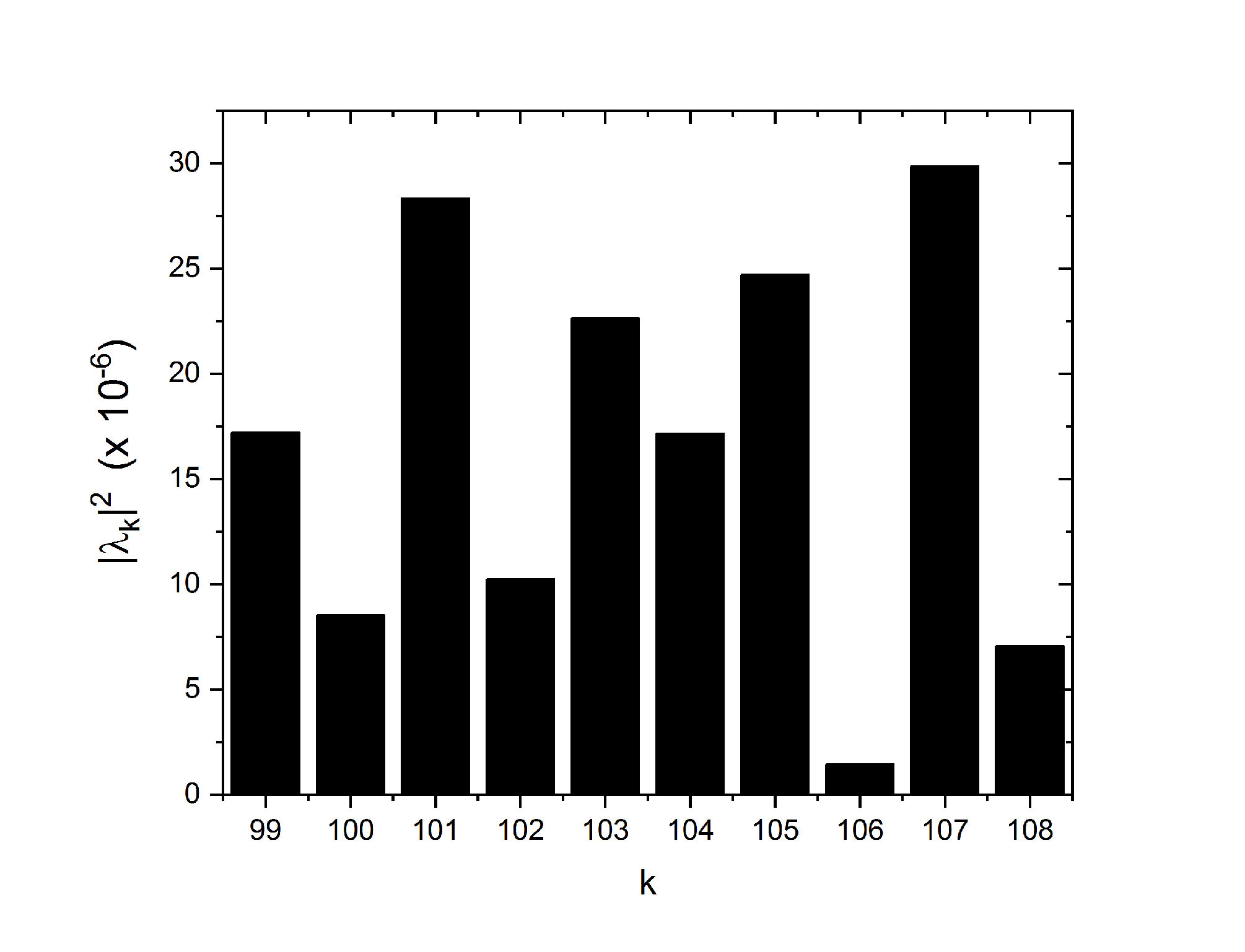
Fig. 3 shows the and calculated for the CEPC lattice, for various integers near (corresponding to the working beam energy at 45.6 ). The amplitude variations are mostly within one order of magnitude. Moreover, evaluation with Eq. (40) of the rate of depolarization with just the two harmonics nearest to the integer part of shows that retaining just those harmonics suffices in most cases in the working energy range of the CEPC.


Then, we employed the SLIM formalism implemented in Bmad to calculate the equilibrium beam polarization as a function of for the CEPC lattice, centered around three working beam energies (45.6 GeV, Z-pole), (80 GeV, WW threshold), and (120 GeV, Higgs), as shown in Fig. 4(a), (b), (c). The step size of is 0.02 in the simulations. For comparison, we also used Eqs.(5), (10) and (40) to evaluate the equilibrium beam polarization analytically, taking into account spin resonances up to the first order. Only the strengths of the two nearest integer spin resonances were retained in the evaluation of Eq. (40). The (numerical) SLIM simulation results match well with the analytical calculations. As the integer spin resonances in the tilt of become much stronger at the working energy for the Higgs particle, the equilibrium beam polarization for the cases with is also much reduced. In addition, there are dips in the equilibrium beam polarization near the first-order “parent” betatron spin resonances, for example when is near at the working energy for Z. But apparently their influence is quite localized, and much weaker compared to the first-order “parent” synchrotron spin resonances. This justifies the analysis of the relative significance of first-order spin resonances in Section II.
We also evaluated the depolarization effects using the theories of the correlated and uncorrelated regimes of spin resonance crossings. We used Eq. (43) to estimate the effect of the correlated resonance crossing, and Eq. (48) to estimate the effect of the uncorrelated resonance crossing, respectively, Then we evaluated Eq. (5) and Eq. (10) to estimate the equilibrium beam polarization of the CEPC lattice. In both cases, we only retained the two Fourier harmonics nearest to the integer part of and for Eq. (43) we retained in the range of -100 to 100 as a result of a check of convergence.
V Results of simulations
In this section we describe the evaluation the depolarization effects of the CEPC lattice using Monte-Carlo Carlo simulations with the PTC code Duan et al. 2015, and compare the results with the predictions of the theories of radiative depolarization, for various lattice settings. In the Monte-Carlo simulations, a bunch of 54 particles was launched on the closed orbit with the same vertical spin, and tracked for 10 damping times in the presence of stochastic photon emissions, but disregarding the Sokolov-Ternov effect. The decay of the beam polarization was recorded, and the data of the calculated beam polarization in the last 8 damping times were fitted to obtain an estimate of the time constant of the spin diffusion . Then the equilibrium beam polarization was estimated through Eq. (5) and Eq. (10).
V.1 Dependence on beam energy
We first studied the variation of the equilibrium beam polarization as a function of near the three operation energies, for Z, WW and Higgs production respectively, as shown in Fig. 5(a), (b) and (c). For the Z and WW energies, the valleys near integers become much wider relative to those in Fig. 4(a) and (b), as predicted by both theories, while the Monte-Carlo simulation results agree better with the theory of the correlated regime, as fine structure of higher-order synchrotron sideband spin resonances is clearly seen. For the Higgs energy, however, although the equilibrium beam polarization level is very low, the results of the Monte-Carlo simulation are quite close to the predictions of the theory of the uncorrelated regime, but are generally higher than the prediction of the theory of the correlated regime, and there are no clear signs of higher-order synchrotron sideband spin resonances.


| Beam energy () | () | () | () | |||||
| 45.6* | 103.5 | 3.77 | 0.028 | 252.72 | 0.03 | 1.39 | ||
| 60.1 | 136.5 | 4.96 | 0.028 | 63.34 | 0.20 | 2.42 | ||
| 69.8 | 158.5 | 5.77 | 0.0324 | 30.00 | 0.36 | 2.82 | ||
| 80.0* | 181.5 | 6.61 | 0.0395 | 15.24 | 0.52 | 3.04 | ||
| 84.4 | 191.5 | 6.97 | 0.0425 | 11.65 | 0.61 | 3.14 | ||
| 90.1 | 204.5 | 7.43 | 0.0467 | 8.39 | 0.72 | 3.25 | ||
| 95.4 | 216.5 | 7.88 | 0.0515 | 6.31 | 0.80 | 3.31 | ||
| 99.8 | 226.5 | 8.24 | 0.0550 | 5.03 | 0.90 | 3.39 | ||
| 109.9 | 249.5 | 9.08 | 0.0585 | 3.10 | 1.48 | 3.87 | ||
| 120.1* | 272.5 | 9.90 | 0.0650 | 2.03 | 1.95 | 4.15 | ||
We then investigated the dependence of the depolarization effects on the beam energy, in the range of 45.6 to 120 . The energy points were selected so that . The total RF voltage was adjusted to compensate for the increase of synchrotron radiation energy loss at higher beam energies and the synchrotron tunes were set to the design values according to the CEPC CDR specifications at 45.6, 80 and 120 . For other beam energy points, the synchrotron tunes were set in a smoothly increasing manner. The related lattice parameters are summarized in Table 4.
Fig. 6 (a) shows the time constant of the spin diffusion obtained by Monte-Carlo simulations, the time constant of the Sokolov-Ternov effect calculated using Bmad, as well as the self-polarization build-up time , at the various beam energies. decreases much faster than with increasing beam energy, as predicted by both Eqs.(43) and (48), and becomes the dominant contributor to at beam energies beyond 85 , This leads to a much reduced level of equilibrium beam polarization at higher beam energies, as shown in Fig. 6 (b). In addition to the results derived from the Monte-Carlo simulations, calculations using the theories of the correlated and uncorrelated regimes are also presented in the figure for comparison. Up to 90 , the simulated equilibrium polarization matches quite well with the theory of the correlated regime, and is smaller than the theory of the uncorrelated regime. However, as the beam energies get even higher, there are nontrivial discrepancies between the results of simulations and the theories. This might suggest the paradigm shift from the correlated regime towards the uncorrelated regime. As shown previously, the results from the Monte-Carlo simulation are close to the theory of the uncorrelated regime at around 120 .
V.2 Influence of asymmetric wigglers at the Z pole
The time constant of the Sokolov-Ternov effect is as large as 253 at Z pole. Using the self-polarization mechanism to generate sufficient beam polarization for RD requires a much reduced polarization build-up time. This can be achieved by implementing asymmetric wiggler magnets Derbenev et al. 1979. This possibility was investigated in detail for LEP Blondel and Jowett 1987, and also studied for the FCC-ee E Gianfelice-Wendt 2016. An asymmetric wiggler consists of three bending magnets. The central bending magnet has a length and a magnetic field in the same direction as the guiding magnetic field in the arcs. Its bending angle is denoted as , while the bending magnets on both sides have equal length , equal magnetic field in the opposite direction to , and equal bending angles . It is required that to ensure no change in the layout and optics beyond the wiggler insertion. When units of such asymmetric wigglers are included into the straight sections of the lattice, in addition to a decrease of , there is also an decrease of , as well as increases in the energy loss per turn , and the rms relative energy spread . A larger leads to a larger modulation index , so that the higher-order synchrotron sideband spin resonances are much enhanced. This could in turn increase and further reduce the equilibrium beam polarization level.
To this end, the influence of asymmetric wigglers on radiative depolarization was evaluated quantitatively. Ten identical units of asymmetric wigglers were inserted into the straight sections of the CEPC lattice Xia et al. 2021, with , , i.e., . In this paper, various settings of and thus were used to study the influence on the depolarization effects. The synchrotron tune was kept fixed at 0.028 by adjusting the total RF voltages.
| wigglers | (rad) | () | () | |||
|---|---|---|---|---|---|---|
| w/o | - | 36.1 | 3.77 | 252.8 | 0.03 | 1.39 |
| Case 1 | 0.0033 | 43.9 | 9.53 | 32.3 | 0.22 | 3.52 |
| Case 2 | 0.0056 | 60.0 | 17.26 | 7.2 | 1.00 | 6.38 |
| Case 3 | 0.0080 | 84.8 | 24.55 | 2.5 | 2.85 | 9.07 |
Table 5 shows the beam parameters for the lattice without wigglers, and three different wiggler settings with increasing . For example, in Case 1, the time constant of the Sokolov-Ternov effect is reduced to about 32 , and then about 2 are needed to obtain 5% beam polarization, more or less sufficient for energy calibrations. Case 2 and Case 3 use even stronger wiggler magnets, and the increase in and is more substantial. Though not relevant for practical use, these cases are employed here out of academic interest. In these three cases, the locations of higher-order synchrotron sideband spin resonances are the same while the theory of the correlated regime predicts lower levels of equilibrium polarization and wider valleys near these resonances for increasing wiggler strengths characterized by . In contrast, as predicted by the theory of the uncorrelated regime, there are no higher-order synchrotron sideband spin resonances, and the equilibrium polarization level is higher for near 103.5 compared to the prediction of the theory of the correlated regime.


Fig. 7 shows the equilibrium beam polarization as a function of for the lattices using these three different wiggler settings. The Monte-Carlo simulation results are compared with the theories of the correlated regime and the uncorrelated regime. Fig. 7(a) shows the outcomes of Case 1 where the Monte-Carlo simulation results fit well with the theory of the correlated regime, with obvious polarization dips in the synchrotron sideband spin resonance regions, which are absent in the theory of the uncorrelated regime. Fig. 7(b) shows the outcomes of Case 2 where the results of the Monte-Carlo simulation are inconsistent with the valleys predicted by the theory of the correlated regime. Fig. 7(c) shows the outcomes of Case 3 where the results of Monte-Carlo simulation show no obvious resonance structures and are generally between the predicted levels of equilibrium beam polarization of the two theories.


These results of the Monte-Carlo simulations indicate deviations from the theory of the correlated regime, when the condition on the correlation index no longer holds, but aren’t in agreement with the theory of the uncorrelated regime either. Using even larger in the lattice setup leads to an RF bucket insufficient for fully capturing the beam particles in the simulations and thus this parameter space was not explored.
In addition, we fixed the beam energy at 45.6 , and scanned to study the dependence of the energy loss per turn, rms relative energy spread, polarization time and equilibrium polarization, as shown in Fig. 8. The results of simulations for the equilibrium polarization match well with the theory of the correlated regime for small settings, however, there is an increasing deviation for larger than 0.004 rad. In the parameter range covered, the results of Monte-Carlo simulation are between the equilibrium polarization levels predicted by the two theories, respectively.
V.3 Influence of RF settings at the Z pole
In the CDR for the CEPC it is assumed that the ring has a single frequency RF system of 650 . Then for a chosen momentum compaction factor, e.g., according to Eq. (3.43) and Eq. (5.66) in Ref. Matthew 1970, the bunch length and synchrotron tune cannot be adjusted separately. However, earlier studies revealed a novel coherent head-tail instability (X-Z instability) induced by the beam-beam interaction at a large Piwinski angle Ohmi et al. 2017; Kuroo et al. 2018, that could be enhanced when longitudinal impedance is also taken into account Zhang et al. 2020; Lin et al. 2022. Thus it was suggested Migliorati et al. 2021 that the instability could be viably mitigated by including a higher-harmonic RF system to lengthen the bunches. It has also been suggested that bunch lengthening can lead to a reduction in the center-of-mass energy spread in collisions. For non-colliding bunches, the introduction of harmonic cavity itself does not help to reduce the rms energy spread. However, for colliding bunches, the rms energy spread of a beam can suffer from a significant increase due to beamstrahlung and the beamstrahlung-induced energy spread can to some extent be alleviated by the introduction of harmonic cavities 22 2 P. Raimondi, “Updates on Monochromatization”, talk on FCC-FS EPOL group and FCCIS WP2.5 meeting 15 (24 Nov 2022), and D. Shatilov and P. Raimondi, “ FCC-ee parameters and Challenges”, talk on FCCIS Workshop 2022 (06 Dec 2022). . Of course, a reduction of the rms energy spread in the beams also reduces the spread in the instantaneous spin-precession rate.
In such a double RF system the synchrotron tune at zero amplitude is different from that of a single RF system and so is the dependence of on the synchrotron amplitude Hofmann and Myers 1980; S. Y. Lee 2004. Since both the modulation index and the correlation index depend on , it’s expected that the radiative depolarization effects can be different.
Although there is currently no plan to use a double RF system for the CEPC, a study of the effect on depolarization with such a system opens up new directions for study which might bare fruit in the future. We therefore now look in detail at the effects of a double-frequency system for the CEPC running near 45.6 GeV.


Simulations with the thick-lens SLIM algorithm in the code SLICKTRACK Barber 2005 for a real ring show that synchrotron motion for a single RF system is close to simple harmonic although the RF cavities are localised. Then it is reasonable, as a first step, to follow the description in Ref. S. Y. Lee 2004 in which the RF system is distributed uniformly. Moreover, only synchrotron motion is included here but the applicability of this model has been confirmed a posteriori with Monte-Carlo simulations with localised cavities as described below.
Thus we begin by writing the voltage seen by beam particles in the presence of a double-frequency RF system as
| (52) |
where is the RF phase of a particle relative to that of the reference particle, and are the total voltage and RF synchronous phase for each RF frequency, with subscripts “1” and “2” denoting the fundamental and the harmonic RF system, respectively, and the integer is the ratio of the harmonic RF frequency to the fundamental RF frequency. The parameters of the double-frequency RF system must be set to compensate for the synchrotron radiation energy loss per turn , this requires
| (53) |
where is the charge of the electron.
There are still 3 degrees of freedom in the parameters of the double RF system. To simplify the discussion in this paper, we study three different cases of RF settings, all these cases feature a single RF bucket and beam particles oscillate around a single “stable” fixed point at . In Case A, we set MV, so that the double RF system effectively reduces to the case of the single RF system. Then we specify as the only independent variable, which is related to the rms bunch length and the RF bucket height. In Case B, we fix rad, so that , and thus the setting of the fundamental RF system is the same as that of a single RF system alone. For a specified , we choose various positive values of that lead to different rms bunch lengths and different dependences of synchrotron tune on the synchrotron amplitude. Note that this reduces to Case A if MV. In Case C, we consider a special type of settings called the “ideal bunch lengthening” condition, with a vanishing slope of the RF wave at the synchronous phase. This requires both the first and second derivatives of the total RF voltage at the synchronous phase be set to zero Hofmann and Myers 1980:
| (54) |
so that
| (55) |
We specify as the only independent variable, all other RF parameters are determined using Eq. V.3.
In the following studies, we use the CEPC lattice with the wiggler settings of Case 1, and consider a fundamental RF system running at 650 and a harmonic RF system running at 1.3 .
But before describing our numerical results for the three different cases of RF settings, we direct the reader to Appendix (Section VII.3) where the mathematical details are presented together with illustrative plots of the regions of stable motion in and and indications of the positions of the unstable fixed points and the turning points. Then, with that formalism, we evaluate the synchrotron tune at various synchrotron amplitudes as well as the equilibrium longitudinal distribution of particles under the influence of damping and excitation by synchrotron radiation. For that we choose a beam energy of 45.72 GeV () and fix MV. Then rad in Case A and Case B. For Case C, rad, MV and rad.
The dependences of on the orbital amplitudes of the three cases are shown in Fig. 9(a) where, as indicated in Appendix (Section VII.3), the amplitudes are represented by the measure . As shown, a larger in Case B leads to a lower at zero synchrotron amplitude relative to that of Case A, and approaches a vanishing at zero synchrotron amplitude in Case C. The latter is expected given that, as mentioned earlier, the slope of the RF wave is zero at the synchronous phase. In addition, is essentially proportional to the amplitude of at small amplitude in Case C and the spread of among beam particles is much larger compared to that of Case A and Case B. As shown in Fig. 9(b), the longitudinal distribution in the presence of damping and synchrotron radiation is Gaussian in Case A, and features a “flat-top” and a much wider distribution in Case C. The distribution becomes wider for increasing in Case B and falls between the distributions of Case A and Case C. In addition, if we choose an even larger (for example 50 MV) in Case B, then is no longer a single stable fixed point that beam particles oscillate around. Instead, there are two stable fixed points within the single RF bucket, so that the longitudinal distribution follows a “double-hump” shape, and the distribution of in terms of would be more complicated. This “over-stretched” regime is discussed in Ref. S. Y. Lee 2004, but is beyond the scope of this paper.
The applicability of the model with a uniform distribution of the RF system is illustrated in Appendix (Section VII.3) where one sees good agreement for Case C between the predictions of the model and the distributions in and from a Monte-Carlo simulations with the two kinds of localised cavities and full synchro-betatron motion.
Now we are ready to present the influence of the various settings of the double RF system on the radiative depolarization effects. For Case A with a single RF system alone, the results of equilibrium polarization for the CEPC have already been shown in Fig. 7(a). Although different settings of the RF voltage and phase were used relative to those of Case A in Fig. 9, the Monte-Carlo simulation results agree with the prediction of the theory of the correlated regime.
For Case C at the ideal bunch lengthening condition, as already shown in Fig. 9(a), the synchrotron tune is zero at zero amplitude. A direct application of Eq. (41), by plugging at zero amplitude, then leads to a vanishing enhancement factor so that the expected equilibrium beam polarization of the theory of the correlated regime is the same as the result of the first-order theory. Meanwhile, the correlation index is infinite and it is expected that the theory of the uncorrelated regime is applicable.
We chose a beam energy of 45.6 GeV, and selected the following parameters of the double RF system to match the ideal bunch lengthening condition: MV, rad, MV and rad. To simplify the treatment, this RF setting was used in the simulations at different beam energies in the range of to . Then the “ideal bunch lengthening” condition is exactly met for , with minor deviations for other beam energies. Fig. 10 shows the equilibrium beam polarization for the CEPC. On one hand, the results of SLIM calculations with equal numbers of both kinds of localized cavities match well with the prediction of the first-order theory. On the other hand, the results of Monte-Carlo simulations are in good agreement with the predictions for the theory of the uncorrelated regime, and are quite different from the predictions of the first-order theory. These results are indeed consistent with the theory of the uncorrelated regime encapsulated in Eq. (48).

We also studied the influence of the double RF settings in Case B to the radiative depolarization effects. Here, we fixed the beam energy at (), where there is a more obvious contrast in the behaviour of the equilibrium beam polarization. We fixed the settings at MV, rad and , and scanned the total voltage of the harmonic RF system from MV up to MV, thus obtaining a range of synchrotron tunes at zero amplitude of synchrotron motion, from 0.028 down to 0.005.
The outcome is shown in Fig. 11 where the equilibrium beam polarization is plotted as a function of the synchrotron tune at zero amplitude and the results of Monte-Carlo simulation are compared with the predictions of the theories. The theory of the uncorrelated regime encapsulated in Eq. (48) predicts that the equilibrium beam polarization is independent of the synchrotron tune, in strong contrast with the prediction of the theory of the correlated regime, whereby a closer examination of Eq. (43) indicates that the equilibrium beam polarization should oscillate as the distance to the nearest higher-order synchrotron sideband spin resonance varies with . Thus the dips correspond to certain higher-order synchrotron sideband spin resonances and as increases, so does the distance between adjacent dips (and adjacent peaks), as well as the peak equilibrium beam polarization. The results of Monte-Carlo simulation match well with the theory of the correlated regime for , and are in line with the theory of the uncorrelated regime for . Between these two extremes, the simulation results suggest a transition from the correlated regime to the uncorrelated regime. The vertical dashed line corresponds to to guide the eye, but we can’t detect a clear boundary between the correlated regime and the uncorrelated regime.

In summary, when the synchrotron tune at zero amplitude is very small, in the presence of a harmonic RF system, the Monte-Carlo simulation results agree well with the theory of the uncorrelated regime. As the synchrotron tune at zero amplitude becomes larger, the Monte-Carlo simulations indicate a gradual transition from the uncorrelated regime to the correlated regime, and match well with the theory of correlated regime when .
As we already mentioned in Section II.B, the theory of the correlated regime was derived under the assumption that the synchrotron motion is approximately harmonic, which is applicable in Case A. However, in the presence of a double-RF system, the synchrotron motion could become nonlinear even at small amplitudes. This is particularly true in Case C. In Case B, as we increase the voltage of the harmonic RF system , the synchrotron motion at small amplitudes becomes more nonlinear and deviates from Case A. However, the nonlinear synchrotron motion of and can still be represented by action-angle variables, but in a much more complicated form involving elliptical functions S. Y. Lee 2004. It is unclear if a simple analytical form of can be obtained following the approach of derivation in Ref. Yokoya 1983 in this context. But it is clear that the application of the theory of correlated regime is limited to the case where the assumption of approximately harmonic synchrotron motion is still valid.
VI Conclusion and outlook
This paper presents a detailed investigation of the radiative depolarization effects in the CEPC. Both theoretical evaluations and Monte-Carlo simulations are employed and compared, for a CEPC CDR lattice seed with detailed error modeling and after dedicated corrections, and for various lattice settings.
The contribution from the first-order “parent” synchrotron spin resonances to radiative depolarization is explicitly derived and its connection to the underlying integer spin resonance strengths is established, for ultra-high energy electron storage rings. This agrees with the expressions in Ref. Derbenev et al. 1979 for a vanishing synchrotron tune. SLIM simulations for the CEPC lattice seed agree well with this first-order theory for various beam energies, and also indicate that the first-order “parent” betatron spin resonances are much weaker compared to the first-order “parent” synchrotron spin resonances.
There are two distinct theories Derbenev et al. 1979 that describe the influence of synchrotron oscillations on radiative depolarization at ultra-high beam energies. The theory of the correlated regime highlights the enhancement of the “parent” spin resonances by higher-order synchrotron sideband spin resonances, while the theory of the uncorrelated regime predicts vanishing resonance structures and a generally higher equilibrium beam polarization level compared to the theory of the correlated regime. Monte-Carlo simulations have been conducted for various beam energies, various settings of asymmetric wigglers at the Z energy, as well as for various settings of harmonic RF cavities. On one hand, these simulation results are in line with the theory of the correlated regime for a correlation index . On the other hand, the simulation of the double-RF system in the ideal lengthening condition are consistent with the theory of the uncorrelated regime, while is infinite by definition. Between these two extremes, the Monte-Carlo simulations of the equilibrium beam polarization are generally between the predictions of these two theories, but are not in line with either. This indicates a gradual evolution from the correlated regime to the uncorrelated regime. A potential theoretical development is foreseen, to achieve a more complete description of the radiative depolarization, that merges into these two theories at extremes.
In that context we make the following observations. Electron and positron storage rings need accelerating cavities in order to replace the particle energy lost by synchrotron radiation. Then the particle dynamics is unavoidably intrinsically time-dependent and that is recognised in Derbenev and Kondratenko 1972; Kondratenko 1974; Derbenev and Kondratenko 1975; Yokoya 1983 among many others. Thus, for example, the vector of the ISF is a function of all six canonical orbital variables as well as . Moreover, as in Beznosov Oleksii 2020, it can be argued that for phase-space equilibrium and for the relatively slow variation of the polarization, the local polarization vector at each point in six-dimensional phase space is parallel to defined on six-dimensional phase space. This is the so-called ISF approximation. However, the ISF in Derbenev and Kondratenko 1973; Derbenev et al. 1979 is defined to be explicitly time-independent. Then in Derbenev et al. 1979 synchrotron motion is added to the dynamics by hand. So what, then, is the direction of at orbital equilibrium in that case? In any case, we expect the ISF approximation to apply in the regime of non-resonant spin diffusion but it perhaps needs verification for the regime of resonant spin diffusion. Moreover, if the ISF is not relevant in the regime of resonant spin diffusion, what is the status of the terms and in the DK formula, Eq. (7)? Should the averages involving in those terms simply be replaced by averages involving as is usually done anyway in practical evaluations of the depolarisation-free asymptotic polarization?
Fortunately, we can now evaluate the validity of the theory behind resonant spin diffusion and uncorrelated resonance crossing at ultra-high energy by following the history of individual spins using Monte-Carlo simulations. So could be set close to, or far away, from resonances and the effects on single spins of large synchrotron amplitude or large photon energy could be studied in detail and perhaps then used to predict the behaviour of ensembles.
Monte-Carlo codes like Bmad can also be used to check and support analytical calculations. For example, it has been seen that some perturbative calculations involving of the rate of depolarization for non-resonant spin diffusion need not converge at high energy as more and more synchrotron sidebands are included S. R. Mane 1990; S. R. Mane 1992b. Then Monte-Carlo simulations should be used instead. Of course, this matter is unrelated to the smoothing away of synchrotron sidebands in the regime of uncorrelated resonance crossing.
We should also note that the so-called Bloch equations Heinemann et al. 2019; Beznosov Oleksii 2020; Heinemann:2020pzl foreseen in Derbenev and Kondratenko 1975 have the potential to expose deviations from the DK formula, Eq. (7), starting from first principles.
We are aware of developments in Bmad, in particular its facility to gain speed by using pre-established spin-orbit maps Nishikawa et al. 2022 for tracking between dipoles where radiation takes place, instead of tracking element-by-element. The increase in computing speed provided by this advanced feature, so-called ”sectioning”, should make it possible in future studies to track with many more particles, to launch finer parameter scans as well as to simulate the resonant depolarization process.
The results presented here refer to a single set of error seeds. Future work, facilitated by sectioning, will employ several sets of error seeds in order to obtain a better overview. For example, ensembles of distortions of and deviations of from will be available. The statistical spread of due to closed-orbit distortions will give insights into how well the beam energy, and then the center-of-mass energy, can be estimated with RD Blondel et al. 2019. In addition, more depolarizing contributors like the detector solenoids, spin rotators to realize longitudinal polarization, and more complete machine imperfection sources, shall be included in future studies. These are important for predicting the achievable beam polarization level, and for establishing methods for realizing a high beam polarization. Note that we didn’t implement dedicated corrections such as in harmonic closed-orbit spin matching schemes Rossmanith and Schmidt 1985; Barber et al. 1994, which decrease the distortion of . Applications of these correction schemes shall be carefully studied in order to optimize the achievable beam polarization, as part of an integrated approach of performance optimization in these future colliders.
As far as we know, no other studies for very high energy go as far as those presented here.
Acknowledgments
W. H. Xia would like to thank S. Nikitin and F. Meot for early guidance in spin dynamics studies. The authors are grateful to D. Sagan and E. Forest for kind help with Bmad/PTC. The authors acknowledge the proofreading and suggestions of S. Nikitin. D. P. Barber thanks K. Heinemann and J.A. Ellison for collaboration on many aspects of spin dynamics. This study was supported by National Key Program for S&T Research and Development (Grant No. 2018YFA0404300 and 2016YFA0400400); National Natural Science Foundation of China (Grant No. 11975252); Key Research Program of Frontier Sciences, CAS (Grant No. QYZDJ-SSW-SLH004); Youth Innovation Promotion Association CAS (No. 2021012).
References
- Abada et al. (2019) A. Abada et al., FCC-ee: The Lepton Collider, Eur. Phys. J. Spec. Top. 228, 261–623 (2019).
- Shiltsev and Zimmermann (2021) V. Shiltsev and F. Zimmermann, Modern and future colliders, Rev. Mod. Phys. 93, 015006 (2021).
- The CEPC Study Group (2018) The CEPC Study Group, CEPC Conceptual Design Report Volume I-Accelerator , arXiv:1890.00285 (2018).
- CEPC Accelerator Study Group (2022) CEPC Accelerator Study Group, Snowmass2021 White Paper AF3-CEPC (2022).
- Derbenev et al. (1980) Y. S. Derbenev et al., Accurate calibration of the beam energy in a storage ring based on measurement of spin precession frequency of polarized particles, Part. Accel. 10, 177 (1980).
- Assmann et al. (1998) R. W. Assmann et al., Calibration of centre-of-mass energies at LEP1 for precise measurements of Z properties, Eur. Phys. J. C 6, 187 (1998).
- Duan et al. (2019) Z. Duan et al., Concepts of longitudinally polarized electron and positron colliding beams in the Circular electron positron collider, in Proc. of IPAC2019, Melbourne, Australia, paper MOPMP012 (2019).
- Xia et al. (2022) W. H. Xia et al., Investigation of spin rotators in CEPC at the Z-pole, Radiation Detection Technology and Methods 6, 490 (2022).
- L H Thomas (1964) L H Thomas, The kinematics of an electron with an axis, Philos. Mag. 3, 1927 (1964).
- Bargmann et al. (1959) V. Bargmann, L. Michel, and V. L. Telegdi, Phys. Rev. Lett. 2, 435 (1959).
- Barber et al. (2004) D. P. Barber, J. Ellison, and K. Heinemann, Quasiperiodic spin-orbit motion and spin tunes in storage rings, Physical Review Special Topics—Accelerators and Beams 7, 124002 (2004).
- Hoffstaetter et al. (2006) G. H. Hoffstaetter et al., Adiabatic invariance of spin-orbit motion in accelerators, Phys. Rev. ST Accel. Beams 9, 014001 (2006).
- Chao (1979) A. W. Chao, Evaluation of beam distribution parameters in an electron storage ring, Journal of Applied Physics 50, 595 (1979).
- Baier et al. (1970) V. N. Baier, V. M. Katkov, and V. M. Strakhovenko, Kinetics of radiative polarization, Sov. Phys. JETP 31, 908 (1970).
- Derbenev and Kondratenko (1973) Y. S. Derbenev and A. M. Kondratenko, Polarization kinematics of particles in storage rings, Sov. Phys. JETP 37, 968 (1973).
- Mane (1987) S. Mane, Electron-spin polarization in high-energy storage rings. I. Derivation of the equilibrium polarization, Physical Review A 36, 105 (1987).
- Baier and Orlov (1966) V. N. Baier and Y. F. Orlov, Quantum depolarization of electrons in a magnetic field, Sov. Phys. Dokl. 10, 1145 (1966).
- Derbenev et al. (1979) Y. S. Derbenev, A. M. Kondratenko, and A. N. Skrinsky, Radiative polarization at ultra-high energies, Particle Accelerators 9, 247 (1979).
- Kondratenko (1974) A. M. Kondratenko, The stability of the polarization of colliding beams, Sov. Phys. JETP. 39, 592 (1974).
- Derbenev and Kondratenko (1975) Y. S. Derbenev and A. M. Kondratenko, Relatixation of the equilibrium state of polarization of electrons in storage rings, Sov. Phys. Dokl. 19, 438 (1975).
- D. P. Barber, G. Ripken (a) D. P. Barber, G. Ripken, Section 2.7.8, Computing Algorithms and Spin Matching, in Handbook of Accelerator Physics and Engineering, A. W. Chao et al. (Eds.), 1st ed., 3rd printing, 2006, World Scientific, Singapore.
- D. P. Barber, G. Ripken (b) D. P. Barber, G. Ripken, Section 2.6.7, Computing Algorithms for Polarization in Storage Rings, in Handbook of Accelerator Physics and Engineering, A. W. Chao et al. (Eds.), 3rd ed., (to be published).
- Chao (1981) A. Chao, Evaluation of radiative spin polarization in an electron storage ring, Nuclear Instruments and Methods in Physics Research 180, 29 (1981).
- S. R. Mane (1987) S. R. Mane, Electron-spin polarization in high-energy storage rings. II. Evaluation of the equilibrium polarization, Phys. Rev. A 36, 120 (1987).
- Yokoya (1992) K. Yokoya, Nonperturbative calculation of equilibrium polarization of stored electron beams, KEK Report KEK-92-6, KEK (1992).
- K. Yokoya (1999) K. Yokoya, An Algorithm for Calculating the Spin Tune in Circular Accelerators, DESY 99-006, arXiv:physics/9902068v1 (1999).
- Yokoya (1987) K. Yokoya, Calculation of the equilibrium polarization of stored electron beams using lie algebra, Nuc. Instrum. and methods in Phys. Research A 258, 149 (1987).
- Kewisch (1985) J. Kewisch, Ph.D thesis, Hamburg University (1985).
- Barber (2005) D. P. Barber, Polarization in the eRHIC Electron(Positron) Ring, in Proc. Spin 2004 (World Scientific, Trieste, Italy, 2005) pp. 738–741.
- (30) D. Sagan et al., The Bmad Reference Manual, https://www.classe.cornell.edu/bmad/manual.html.
- Assmann et al. (2001) R. Assmann et al., Spin dynamics in LEP with 40-100 GeV beams, AIP Conf. Proc. 570, 169 (2001).
- Mane (2014) S. R. Mane, Polarization at TLEP/FCC-ee: ideas and estimates, arXiv:1406.0561 (2014).
- Nikitin (2019) S. A. Nikitin, Opportunities to obtain polarization at CEPC, International Journal of Modern Physics A 34, 1940004 (2019).
- S. A. Nikitin (2020) S. A. Nikitin, Polarization issues in circular electron–positron super-colliders, International Journal of Modern Physics A 35 (2020).
- Heinemann et al. (2019) K. Heinemann et al., The Bloch equation for spin dynamics in electron storage rings: Computational and theoretical aspects, International Journal of Modern Physics A 34, 1942032 (2019).
- Beznosov Oleksii (2020) Beznosov Oleksii, From Wave Propagation to Spin Dynamics: Mathematical and Computational Aspects, Ph.D. thesis, University of New Mexico (2020).
- K. Heinemann and others (2020) K. Heinemann and others, Int. J. Mod. Phys. A 35, 2041003 (2020).
- E Gianfelice-Wendt (2016) E Gianfelice-Wendt, Phys. Rev. Accel. Beams 19, 101005 (2016).
- Koop (2018) I. A. Koop, Resonant Depolarization at Z and W at FCC-ee, Proceeding of eeFACT 2018, TUPBB04 , 165 (2018).
- Forest et al. (2002) E. Forest, F. Schmidt, and E. McIntosh, Introduction to the Polymorphic Tracking Code, CERN-SL-2002-044 (AP), and KEK-Report 2002-3 (2002), https://frs.web.cern.ch/frs/report/sl-2002-044.pdf.
- (41) E. Forest, FPP Manual, https://usermanual.wiki/Document/fppmanual.653439610/help.
- Duan et al. (2015) Z. Duan, M. Bai, D. P. Barber, and Q. Qin, A Monte-Carlo simulation of the equilibrium beam polarization in ultra-high energy electron (positron) storage rings, Nuc. Instrum. and methods in Phys. Research A 793, 81 (2015).
- Yokoya (1983) K. Yokoya, Spin chromaticity for higher-order synchrotron resonances , Particle accelerators 13, 85 (1983).
- Yokoya (1986) K. Yokoya, Beam polarization in high energy electron storage rings , KEK Report 85-7, KEK (1986).
- Hoffstaetter (2006) G. H. Hoffstaetter, High-Energy Polarized Proton Beams, Springer Tracts in Modern Physics, Vol. 218 (Springer New York, New York, NY, 2006).
- Hoffstatter et al. (1999) G. H. Hoffstatter, M. Vogt, and D. P. Barber, Higher order effects in polarized proton dynamics, Physical Review Accelerators and Beams 2, 114001 (1999).
- M. Vogt (2000) M. Vogt, Bounds on the Maximum Attainable Equilibrium Spin Polarization of Protons at High Energy in HERA, Ph.D. thesis, University of Hamburg (2000).
- Lee (1997) S. Y. Lee, Spin dynamics and snakes in synchrotrons (World Scientific, 1997).
- (49) Note, however, that the Eq. 3.3 in Ref. Derbenev et al. 1979 suffers from an error whereby the exponent in the denominator should be 4 instead of 2.
- A. M. Kondratenko (1982) A. M. Kondratenko, Radiative polarization in storage rings, BINP Preprint 82-28 (1982).
- Montague (1984) B. Montague, Polarized beams in high energy storage rings, Physics Reports 113, 1 (1984).
- Rossmanith and Schmidt (1985) R. Rossmanith and R. Schmidt, Compensation of Depolarizing Effects in Electron-Positron Storage Rings, Nuclear Instruments and Methods in Physics Research Section A: Accelerators, Spectrometers, Detectors and Associated Equipment 236, 231 (1985).
- Barber et al. (1994) D. Barber et al., High Spin Polarization at the HERA Electron Storage Ring, Nuclear Instruments and Methods in Physics Research Section A: Accelerators, Spectrometers, Detectors and Associated Equipment 338, 166 (1994).
- Assmann et al. (1995) R. Assmann, A. Blondel, B. Dehning, et al., Lepton Beam Polarization at LEP, in AIP Conference Proceedings, Vol. 343 (1995) pp. 219–229.
- S. R. Mane (1990) S. R. Mane, Synchrotron Sideband Spin Resonances in High-energy Electron Storage Rings, Nuclear Instruments and Methods in Physics Research A 292, 52 (1990).
- S. R. Mane (1992a) S. R. Mane, Polarization of electron beams in high energy storage rings Part I. Convergence of perturbation theory, Nuclear Instruments and Methods in Physics Research A 321, 21 (1992a).
- S. R. Mane (1992b) S. R. Mane, Polarization of electron beams in high energy storage rings. Part II. Series expansion with tune modulation, Nuclear Instruments and Methods in Physics Research Section A 321, 42 (1992b).
- Wang et al. (2021) B. Wang et al., A Correction Scheme for the Magnet Imperfection on the CEPC Collider Ring, in Proc. of IPAC2021, paper TUPAB007 , 1346 (2021).
- (59) SAD Home Page, https://acc-physics.kek.jp/SAD/.
- A. Terebilo (2001) A. Terebilo, Accelerator toolbox for MATLAB, SLAC-PUB-8732 (2001).
- Zhou et al. (2016) D. Zhou et al., Lattice translation between accelerator simulation codes for SuperKEKB, in Proc. of IPAC2016, Busan, Korea, paper WEPOY040 (2016).
- Blondel and Jowett (1987) A. Blondel and J. M. Jowett, Wigglers for polarization, Conf. Proc. C8711093 216 (1987).
- Xia et al. (2021) W. Xia, J. Gao, Y. Wang, et al., CEPC Z-pole polarization design studies, International Journal of Modern Physics A , 2142003 (2021).
- Matthew (1970) S. Matthew, The Physics of Electron Storage Rings An Introduction, SLAC Report No. 121 (1970).
- Ohmi et al. (2017) K. Ohmi, N. Kuroo, K. Oide, et al., Coherent Beam-Beam Instability in Collisions with a Large Crossing Angle, Physical Review Letters 119, 134801 (2017).
- Kuroo et al. (2018) N. Kuroo, K. Ohmi, K. Oide, et al., Cross-wake force and correlated head-tail instability in beam-beam collisions with a large crossing angle, Physical Review Accelerators and Beams 21, 031002 (2018).
- Zhang et al. (2020) Y. Zhang, N. Wang, C. Lin, et al., Self-consistent simulations of beam-beam interaction in future circular colliders including beamstrahlung and longitudinal coupling impedance, Physical Review Accelerators and Beams 23, 104402 (2020).
- Lin et al. (2022) C. Lin, K. Ohmi, and Y. Zhang, Coupling effects of beam-beam interaction and longitudinal impedance, Physical Review Accelerators and Beams 25, 011001 (2022).
- Migliorati et al. (2021) M. Migliorati, E. Carideo, D. Arcangelis, et al., The European Physical Journal Plus 136, 1190 (2021).
- (70) P. Raimondi, “Updates on Monochromatization”, talk on FCC-FS EPOL group and FCCIS WP2.5 meeting 15 (24 Nov 2022), and D. Shatilov and P. Raimondi, “ FCC-ee parameters and Challenges”, talk on FCCIS Workshop 2022 (06 Dec 2022).
- Hofmann and Myers (1980) A. Hofmann and S. Myers, Beam Dynamics in a Double RF System, Experientia 40, 610 (1980).
- S. Y. Lee (2004) S. Y. Lee, Accelerator physics, 2nd ed ed. (World Scientific, Hackensack, N.J, 2004).
- Derbenev and Kondratenko (1972) Y. S. Derbenev and A. M. Kondratenko, Diffusion of Particle Spin in Storage Rings, Sov. Phys. JETP 35, 230 (1972).
- Nishikawa et al. (2022) P. Nishikawa, D. Sagan, and G. H. Hoffstaetter, Using Taylor Maps with Synchrotron Radiation Effects Included, Proc. IPAC 2022 WEPOMS053, 2376 (2022).
- Blondel et al. (2019) A. Blondel et al., Polarization and Centre-of-mass Energy Calibration at FCC-ee, arXiv:1909.12245 (2019).
- J. M. Jowett (1987) J. M. Jowett, Introductory statistical mechanics for electron storage rings, AIP Conference Proceedings 153, 864 (1987).
- Ohmi et al. (1994) K. Ohmi, K. Hirata, and K. Oide, From the beam-envelope matrix to synchrotron-radiation integrals, Physical Review E 49, 751 (1994).
VII Appendix
VII.1 The calculation of
can be expanded in terms of , and as
| (56) |
where . In fact, it can be shown that due to the orthonormality of and . Consider that is in the horizontal plane, while ,
| (57) |
Putting Eq. (56) into the Thomas-BMT equation Eq. (2) on the closed orbit, we find
| (58) |
then the solution of is
| (59) | |||||
Here . is the component of along the direction and represents the influence of the radial magnetic field.
Then, the integrand of Eq. (59) can be expanded into Fourier series,
| (60) |
is the complex strength of the integer spin resonance,
| (61) |
Eq. (59) can be simplified to the following form,
| (62) |
Note that the denominators in this expression are an artefact of the approximations used here and that this expression must be used with care when is near an integer to avoid invalidating the approximations.
VII.2 of an ultra-high-energy electron storage ring
The Fourier harmonic of the vertical component of is
| (63) |

Let us consider an ultra-high-energy electron storage ring lattice composed of superperiods, where each superperiod contains a straight section with a length which is dispersion free, and an arc including FODO cells with half length with the following structure [ QF/2 B QD B QF/2 ].


Then, following the treatment of S. Y. Lee Lee 1997, the Fourier harmonic becomes
| (64) | |||||
where the enhancement function is given by
| (65) |
and where is a positive integer and . Fig. 12 shows for several different . The following are some key properties of
- •
when while
- •
, as approaches an integer
- •
for , for , where is the integer nearest to .
Taking the thin lens approximation, the dispersion functions at the center of the focusing quadrupole (QF) and defocusing quadrupole (QD) of a FODO cell are
| (66) |
where and are the focal lengths of QF and QD, respectively. is the dipole bending angle in each half FODO cell: . Note that with , for small ,
| (67) |
For , the enhancement functions amount to , so that . Then we consider with , i.e., the influence of the enhancement functions.
At ultra-high beam energies, the total length of straight sections only occupies a small fraction of the ring circumference , since a high filling factor of dipoles is required to reduce the synchrotron radiation energy loss. Taking the CEPC lattice as an example, the fraction is 0.18.
becomes only for and is otherwise 0. In contrast, approaches when approaches an integer , but is less than when and . In addition, only a few near the integer part of have significant influence in Eq. (34). The contribution of terms with very large is further suppressed by the term in the denominator. Therefore, we can retain only in Eq. (34) as a reasonable approximation.
As an illustration, Fig. 13 shows the results of simulation for for various , using the CEPC lattice. The CEPC lattice includes 8 interleaved arc sections and straight sections. Each arc section contains 145 regular FODO cells and 4 FODO cells with half bending angles as dispersion suppressors. In effect and . Then peaks of occur when is near , , agreeing with the observation in the lower plot of Fig. 13. However, the 8 straight sections have different functions and thus different lengths. There are also chromatic-correction sections with dipoles in the final focus systems. These are different from the model that we analyzed, and somehow break the symmetry so that Fourier harmonics other than have comparable strengths, as shown in the upper plot of Fig. 13. Nevertheless, the conclusion of our analysis still applies for the CEPC lattice, namely that the contribution of in Eq. (34) is much larger compared to other Fourier harmonics.
VII.3 More detailed theory of a double-frequency RF system
Our treatment of double RF systems follows the treatment in Chapter 3 of Ref. S. Y. Lee 2004, but here and elsewhere we use a different convention for , whereby is the RF phase of a particle relative to that of the reference particle, rather than the phase coordinate relative to the fundamental RF system in Ref. S. Y. Lee 2004. Then .
Then with time as an independent variable, without considering radiation damping and quantum excitation, the equations of motion are
| (68) | |||||
where , , is the momentum compaction factor and is the harmonic number of the fundamental RF system. Equivalently, a particle’s longitudinal motion is described by the Hamiltonian
| (69) | |||||
This is a constant of motion for each particle and it is helpful to think of the term with as being analogous to a kinetic energy whereas the term with can be thought of as a potential energy while the Hamiltonion is analogous to a total energy.
To understand the synchrotron motion, one starts by solving for the fixed points, i.e., the solution of such that
| (70) |
In our convention, we choose as one such fixed point. Then the parameters of the double-frequency RF system must be set to compensate for the synchrotron-radiation energy loss per turn , this leads to Eq. (53). In the case of a single RF system, this is a stable fixed point around which small amplitude particles execute synchrotron oscillations. Besides, there is an unstable fixed point at , which corresponds to the maximum value of the Hamiltonian, i.e., boundary of the RF bucket.
In the case of a double RF system, the number and locations of the fixed points can be obtained by numerically solving Eq. (VII.3). In this paper, we focus on the cases with two fixed points, a stable fixed point at and an unstable fixed point at . The torus that passes through the unstable fixed point is called the separatrix. This separates phase space into regions of bound and unbound motions. We only study particle motion around the stable fixed point, and within the boundary of the RF bucket enclosed by the separatrix, i.e., just the bound motion. Besides the unstable fixed point, there is another special point on the separatrix, , namely the turning point at which the “kinetic energy” is zero and the “potential energy” is the ”total energy”. Since the beam energy range is well above the transition energy in this paper, i.e., , then . Separatrices for Cases A, B and C with our settings are shown in Fig. 14 together with their unstable fixed points and their turning points. We see that for Case C the stable region in is indeed larger than in cases A and B. All three are mirror-symmetric across the axis.

Longitudinal phase space trajectories of particles follow Hamiltonian torii , where is a constant of motion on a torus. The trajectories are also mirror-symmetric across the axis. Then with Eq. (VII.3), an is the “potential energy” for the phase coordinates and with () at which “kinetic energy” is zero, namely at . On the other hand, the maximum “kinetic energy” written as occurs at the minimum of the “potential energy”, namely at where . Then
| (71) |
so that expresses the amplitude of the synchrotron motion in terms of , or .
Eq. (VII.3) can be written as
Then the synchrotron oscillation period can be obtained by using this to integrate the first equation of Eq. (VII.3):
| (72) |
This can be numerically evaluated for a specified , so that we can then obtain the synchrotron tunes, , plotted in Fig. 9a. For each , a measure of the maximum longitudinal distance of a particle from the center of the bunch is and this, being more recognisable, is used instead of as the horizontal axis in Fig. 9(a).
In the presence of radiation damping and quantum excitation, the longitudinal phase-space distribution settles to an equilibrium given by the static solution of the Fokker-Planck equation J. M. Jowett 1987, namely, . This distribution is approximately Gaussian in with an rms relative energy spread , while the distribution of is
| (73) |
where is a normalization factor chosen so that . The first-order and second-order beam moments can be numerically evaluated by
| (74) |
The longitudinal distributions, , are shown in Fig. 9(b), and are obtained by numerically evaluating the r.h.s. of Eq. (73). The horizontal axis in Fig. 9(b) is the longitudinal coordinate . The rms bunch length is then
| (75) |
Note that the second-order beam moments at equilibrium are usually calculated using the beam-envelope matrix as in Ohmi et al. 1994. That method is still applicable for calculation of the rms energy spread, but it fails to deliver the correct rms bunch length in the presence of a double-RF system, because now contains components higher than second order in , which are not properly taken into account by that method. In this case, one can use Eq. (74) and Eq. (75) to numerically evaluate , or use Monte-Carlo simulation to obtain .
In any case, Fig. 15 shows the probability density functions (PDF) of the beam distributions in and , for Case C at the ideal lengthening condition, where the theoretical distributions match well with the histograms from the final beam distribution of a Monte-Carlo simulation with localised cavities and full synchro-betatron motion tracking with 4000 particles for 10 damping times (about 25000 turns). The beam energy is set to 45.72 GeV () and MV.

