跳到论文正文
W Papers独立论文阅读器 arXiv:2204.12676 论文正文 计算阅读时间 · 0%
引用这篇论文根据当前论文元数据生成,正式投稿前建议核对。


License: arXiv.org perpetual non-exclusive license
arXiv:2204.12676v3 [cs.LG] 26 May 2023

The multimarginal optimal transport formulation of adversarial multiclass classificationThanks: Acknowledgements: All authors contributed equally and their names are listed in alphabetic order. This paper is a preprint version of a paper that will appear in JMLR. Part of this work was completed while the authors were visiting the Simons Institute to participate in the program “Geometric Methods in Optimization and Sampling” during the Fall of 2021. The authors would like to thank the institute for hospitality and support. The authors would also like to thank Camilo A. García Trillos, Ryan Murray, and Meyer Scetbon for enlightening conversations on the topics discussed in this work. NGT was supported by NSF-DMS grant 2005797, and together with JK would also like to thank the IFDS at UW-Madison and NSF through TRIPODS grant 2023239 for their support.

Nicolás García Trillos Address: Department of Statistics, University of Wisconsin-Madison, 1300 University Avenue, Madison, Wisconsin 53706, USA. Email address: garciatrillo@wisc.edu , Matt Jacobs Address: Department of Mathematics, Purdue University, Mathematical Sciences Bldg, 150 N University St, West Lafayette, IN 47907 Email address: jacob225@purdue.edu and Jakwang Kim Address: Department of Statistics, University of Wisconsin-Madison, 1300 University Avenue, Madison, Wisconsin 53706, USA. Email address: kim836@wisc.edu
Date: August 11, 2026
Abstract.

We study a family of adversarial multiclass classification problems and provide equivalent reformulations in terms of: 1) a family of generalized barycenter problems introduced in the paper and 2) a family of multimarginal optimal transport problems where the number of marginals is equal to the number of classes in the original classification problem. These new theoretical results reveal a rich geometric structure of adversarial learning problems in multiclass classification and extend recent results restricted to the binary classification setting. A direct computational implication of our results is that by solving either the barycenter problem and its dual, or the MOT problem and its dual, we can recover the optimal robust classification rule and the optimal adversarial strategy for the original adversarial problem. Examples with synthetic and real data illustrate our results.

Key words and phrases:
Adversarial learning, Multiclass classification, Optimal transport, Multimarginal optimal transport, Wasserstein barycenter, Generalized barycenter problem

1. Introduction

In this paper we study, from analytical and geometric perspectives, the problem of adversarial learning in multiclass classification. By multiclass classification we mean the task of assigning classes i^\hat{i} in a set of KK available classes to all inputs x^\hat{x} in some feature space 𝒳{\mathcal{X}} based on the observation of training pairs z=(x,i)z=(x,i). The adversarial component of the problem refers to the desire of producing classification rules that are robust to data perturbations. Mathematically speaking, this means studying optimization problems of the form:

(1.1) inff∈ℱsupμ~∈𝒫⁡(𝒵){R⁡(f,μ~)−C⁡(μ,μ~)}.\inf_{f\in\mathcal{F}}\sup_{\widetilde{\mu}\in\mathcal{P}(\mathcal{Z})}\left\{R(f,\widetilde{\mu})-C(\mu,\widetilde{\mu})\right\}.

Here, ℱ\mathcal{F} denotes the set of all probabilistic multiclass classifiers —see section 2; μ\mu denotes the observed data distribution, which in general is some probability measure on the space 𝒵=𝒳×{1,…,K}\mathcal{Z}={\mathcal{X}}\times\{1,\dots,K\}, but which for simplicity can be thought of as an empirical measure associated to a finite training data set; CC represents a notion of “distance” between data distributions; R⁡(f,μ~)R(f,\widetilde{\mu}) is a risk functional relative to a data distribution μ~\widetilde{\mu} (thought of as a perturbation of μ\mu) and a choice of loss function, which in this paper will be restricted to be the 00-11 loss. Problem (1.1) can be interpreted as a game between a learner and an adversary: the learner’s goal is to find a classifier with small risk, while the adversary tries to find a data perturbation μ~\widetilde{\mu} that makes the risk for the learner large. The adversary has an implicit budget to perform their actions: the adversary can not choose a μ~\widetilde{\mu} that is too far away (relative to CC) from the original data distribution μ\mu.

For a large family of functionals CC in (1.1) we show that the adversarial problem (1.1) is equivalent to a multimarginal optimal transport problem (MOT) of the form:

(1.2) infπ∈ΠK​(μ)∫𝐜⁡(z1,…,zK)​𝑑π​(z1,…,zK),\inf_{\pi\in\Pi_{K}(\mu)}\int\mathbf{c}(z_{1},\dots,z_{K})d\pi(z_{1},\dots,z_{K}),

where 𝐜\mathbf{c} is a cost function discussed in detail throughout the paper and ΠK​(μ)\Pi_{K}(\mu) is a space of couplings specified in section 2.1. As part of this equivalence, we explicitly describe how to construct solutions to the original problem (1.1) from solutions to the problem (1.2) and its dual, offering in this way new computational strategies for solving problem (1.1). Since most algorithms for OT are primal-dual (i.e., they simultaneously search for solutions to both the primal OT problem and its dual), it is actually possible to construct a saddle solution (f∗,μ∗)(f^{*},\mu^{*}) for (1.1) by running one such OT algorithm. The equivalence between (1.1) and (1.2) that we study here is an extension to the multi-class case of a series of recent results connecting adversarial learning in binary classification with optimal transport: [BCM19, Nak19, PJ21a, PJ21b, GM22].

In order to establish the equivalence between (1.1) and (1.2), we develop another interesting equivalent reformulation of (1.1) that reveals a rich geometric structure of the original adversarial problem. This reformulation takes the form of a generalized barycenter problem

infλ,μ~1,…,μ~Kλ⁡(𝒳)+∑i∈[K]C⁡(μi,μ~i)s.t.​λ≥μ~i,i∈[K],\inf_{\lambda,\widetilde{\mu}_{1},\ldots,\widetilde{\mu}_{K}}\lambda(\mathcal{X})+\sum_{i\in[K]}C(\mu_{i},\widetilde{\mu}_{i})\quad\textup{s.t.}\;\lambda\geq\widetilde{\mu}_{i},i\in[K],

which is a novel variant of the Wasserstein barycenter problems introduced in [AC11, CE10]. In the classical Wasserstein barycenter problem, given KK probability measures ϱ1,…,ϱK\varrho_{1},\ldots,\varrho_{K} defined over a Polish space 𝒳\mathcal{X} and a cost c:𝒳×𝒳→[0,∞]c:\mathcal{X}\times\mathcal{X}\to[0,\infty], one tries to find a probability measure ϱ\varrho such that the summed cost of transporting each of the ϱi\varrho_{i} onto ϱ\varrho is as small as possible. In our generalized problem, we try to find a nonnegative measure λ\lambda (no longer necessarily a probability measure) such that the total mass of λ\lambda plus the summed cost of transporting each μi\mu_{i} (not necessarily having the same total mass) onto some part of λ\lambda is as small as possible. Here transporting a μi\mu_{i} onto some part of λ\lambda means we want to find a measure μ~i≤λ\widetilde{\mu}_{i}\leq\lambda and transport μi\mu_{i} to μ~i\widetilde{\mu}_{i} in the classical optimal transport sense. This problem will be studied in detail in section 3. We prove that these generalized barycenter problems can be written as appropriate MOT problems, a result that is analogous to ones in [AC11, CE10] for standard Wasserstein barycenter problems.

From the equivalence with the generalized barycenter problem we will be able to deduce that optimal adversarial attacks can always be obtained as suitable barycenters of KK or less points in the original training data set. Also, from this reformulation we will be able to recognize the structure of the cost function 𝐜\mathbf{c} in (1.2): for the adversary to obtain their optimal strategy, they can actually localize their problem to sets of KK or fewer data points —see section 2.1. Other theoretical, methodological, and computational implications of these reformulations will be pursued in future work. See section 6 for a discussion on future directions for research.

In contrast to many of the existing applications of OT to ML, it is worth emphasizing that in this work OT arises naturally in connection with a learning problem, rather than as a particular way to address a certain machine learning task. For the growing literature in multimarginal optimal transportation this paper offers new examples of cost functions worthy of study. MOT is a rich topic that has been developed over the years from theoretical and applied perspectives. After the first mathematical analysis of general MOT problems in [GS98], there have been numerous subsequent papers establishing geometric and analytic results (e.g., [KP13, Pas15, KP15, CMP17]) for MOT problems. MOT problems have also been used extensively in applications. For example, they appear in the so-called density functional theory in physics [SGGS07, BDPGG12, CFK13, ML13, CDPDM15], and in economics [Eke05, CMN10, CE10]. In the machine learning community, researchers have recently explored many interesting applications, including generative adversarial networks(GANs) [CCK+18, CMZ+19] and Wasserstein Barycenters [AC11, CD14, BCC+15, COO15, SLD18, DD20], where MOTs are used. Recent works like [DMG20, HRCK21] develop a connection between the Schrödinger bridge problem and MOT. MOT problems have been extended to the unbalanced setting —see [BvLNS21].

1.1. Outline of paper

The rest of the paper is organized as follows. In section 2, we introduce most mathematical objects and notation used throughout the rest of the paper. We also introduce the generalized Wasserstein barycenter problem, which can be interpreted as dual of the original adversarial problem (1.1), and define in detail the MOT problem (1.2). In section 3, we study the aforementioned generalized Wasserstein barycenter problem and prove its equivalence with 1) a stratified barycenter problem and 2) a first version of an MOT problem. In section 4 we discuss the equivalence between (1.1) and (1.2) through the duality results in earlier sections. In section 5, we present a collection of examples and numerical experiments whose goal is to illustrate the theory developed throughout the paper and provide further insights into the geometric structure of adversarial learning in multiclass classification. Finally, we wrap-up the paper in section 6 by presenting some conclusions and discussing some future directions for research.

2. Preliminaries

Throughout the paper (𝒳,d)(\mathcal{X},d) will be a Polish space, [K]:={1,…,K}[K]:=\{1,\dots,K\} with K≥2K\geq 2, and 𝒵:=𝒳×[K]\mathcal{Z}:=\mathcal{X}\times[K]. We regard 𝒳\mathcal{X} as the feature space of our learning problem and [K][K] as the set of classes or labels.

Let μ\mu be a finite positive Borel measure (not necessarily a probability measure) over 𝒵\mathcal{Z}. Given i∈[K]i\in[K], we use μi\mu_{i} to represent the positive measure over 𝒳{\mathcal{X}} defined as

(2.1) μi​(A):=μ⁡(A×{i}),\mu_{i}(A):=\mu\left(A\times\{i\}\right),

for all measurable subsets AA of 𝒳{\mathcal{X}}. In the sequel, we use μ\mu to represent a fixed data distribution, which we regard as an observed data distribution or training data distribution, and use μ~\widetilde{\mu} to represent any other arbitrary finite positive measure over 𝒵\mathcal{Z}. Through this paper we use ℳ+​(𝒳)\mathcal{M}_{+}(\mathcal{X}) and ℳ+​(𝒵)\mathcal{M}_{+}(\mathcal{Z}) to denote the set of finite positive (Borel) measures over 𝒳\mathcal{X} and 𝒵\mathcal{Z}, respectively.

Through this paper, the cost function in (1.1) will take the form:

C⁡(μ,μ~):=min⁡∫π∈Γ⁡(μ,μ~)⁡c𝒵​(z,z~)​𝑑π​(z,z~),C(\mu,\widetilde{\mu}):=\min_{\pi\in\Gamma(\mu,\widetilde{\mu})}\int c_{\mathcal{Z}}(z,\tilde{z})d\pi(z,\tilde{z}),

for some cost function c𝒵:𝒵×𝒵→[0,∞]c_{\mathcal{Z}}:\mathcal{Z}\times\mathcal{Z}\rightarrow[0,\infty]. Here and in the remainder of the paper the set Γ⁡(⋅,⋅)\Gamma(\cdot,\cdot) represents the set of couplings between two positive measures over the same space; for example, Γ⁡(μ,μ~)\Gamma(\mu,\widetilde{\mu}) denotes the set of positive measures over 𝒵×𝒵\mathcal{Z}\times\mathcal{Z} with first marginal equal to μ\mu and second marginal equal to μ~\widetilde{\mu}.

Assumption 2.1.

The function c𝒵c_{\mathcal{Z}} will be assumed to have the following structure:

c𝒵​(z,z~)={c⁡(x,x~) if ​i=i~∞ if ​i≠i~,c_{\mathcal{Z}}(z,\tilde{z})=\begin{cases}c(x,\tilde{x})&\quad\text{ if }i=\tilde{i}\\ \infty&\quad\text{ if }i\not=\tilde{i},\end{cases}

for some lower semi-continuous function c:𝒳×𝒳→[0,∞]c:{\mathcal{X}}\times{\mathcal{X}}\rightarrow[0,\infty].

The function cc will be further assumed to satisfy c⁡(x,x)=0c(x,x)=0 for all x∈𝒳x\in\mathcal{X} and the following compactness and coercivity properties:

  • •

    if {xn}n∈ℕ\{x_{n}\}_{n\in\mathbb{N}} is a bounded sequence in (𝒳,d)({\mathcal{X}},d) and {xn′}n∈ℕ\{x_{n}^{\prime}\}_{n\in\mathbb{N}} is a sequence in 𝒳{\mathcal{X}} satisfying supn∈ℕc⁡(xn′,xn)<∞\sup_{n\in\mathbb{N}}c(x_{n}^{\prime},x_{n})<\infty, then {(xn′,xn)}n∈ℕ\{(x_{n}^{\prime},x_{n})\}_{n\in\mathbb{N}} is precompact in 𝒳×𝒳{\mathcal{X}}\times{\mathcal{X}} (with the induced product metric).

The structure of c𝒵c_{\mathcal{Z}} described in Assumption 2.1 is standard in the literature of adversarial learning and can be motivated by the fact that in many applications of interest it is natural to think that the “true” label associated to a perturbation x~\tilde{x} of a data point xx coincides with the true label of the original xx. Naturally, this is simply a modeling choice, and other cost structures of interest can be studied elsewhere. The lower semicontinuity and compactness assumptions on cc are technical requirements that we use in the remainder. All cost functions of interest satisfy these properties —see the examples below.

If we decompose μ\mu and μ~\widetilde{\mu} into measures μi,μ~i\mu_{i},\widetilde{\mu}_{i} as in (2.1), it is possible to write C⁡(μ,μ~)C(\mu,\widetilde{\mu}) as

C⁡(μ,μ~)=∑i∈[K]C⁡(μi,μ~i),C(\mu,\widetilde{\mu})=\sum_{i\in[K]}C(\mu_{i},\widetilde{\mu}_{i}),

abusing notation slightly and interpreting C⁡(μi,μ~i)C(\mu_{i},\widetilde{\mu}_{i}) as

(2.2) C⁡(μi,μ~i)=min⁡∫π∈Γ⁡(μi,μ~i)⁡c⁡(x,x~)​𝑑π​(x,x~).C(\mu_{i},\widetilde{\mu}_{i})=\min_{\pi\in\Gamma(\mu_{i},\widetilde{\mu}_{i})}\int c(x,\tilde{x})d\pi(x,\tilde{x}).
Remark 2.2.

Let us emphasize that we define C⁡(μi,μ~i)=+∞C(\mu_{i},\widetilde{\mu}_{i})=+\infty whenever the set of couplings Γ⁡(μ~i,μi)\Gamma(\widetilde{\mu}_{i},\mu_{i}) is empty, which is the case if μi\mu_{i} and μ~i\widetilde{\mu}_{i} have different total mass.

We introduce two notions that will be used throughout our analysis. Given a lower semi-continuous function f:𝒳→ℝf:\mathcal{X}\to\mathbb{R}, we define

(2.3) fc​(x):=infx′∈𝒳{f⁡(x′)+c⁡(x′,x)},f^{c}(x):=\inf_{x^{\prime}\in\mathcal{X}}\{f(x^{\prime})+c(x^{\prime},x)\},

and given an upper semi-continuous function g:𝒳→ℝg:\mathcal{X}\to\mathbb{R}, we define

(2.4) gc¯​(x′):=supx∈𝒳{g⁡(x)−c⁡(x′,x)}.g^{\bar{c}}(x^{\prime}):=\sup_{x\in\mathcal{X}}\{g(x)-c(x^{\prime},x)\}.
Example 2.3.

Let ε>0\varepsilon>0 and let c⁡(x,x~)c(x,\tilde{x}) be given by

c⁡(x,x~)=cε​(x,x~)={0 if ​d​(x,x~)≤ε∞ if ​d​(x,x~)>ε.c(x,\tilde{x})=c_{\varepsilon}(x,\tilde{x})=\begin{cases}0&\text{ if }d(x,\tilde{x})\leq\varepsilon\\ \infty&\text{ if }d(x,\tilde{x})>\varepsilon\end{cases}.

The parameter ε\varepsilon can be interpreted as the adversarial budget: the larger the value of ε\varepsilon, the wider the space of actions available to the adversary. The cost cc satisfies Assumption 2.1 provided that closed balls with finite radius in (𝒳,d)({\mathcal{X}},d) are compact.

Notice that in this case, the cc-transform fcf^{c} of a given function ff takes the form:

fc(x)=infx′:d⁡(x,x′)≤εf(x′).f^{c}(x)=\inf_{x^{\prime}\>:\>d(x,x^{\prime})\leq\varepsilon}f(x^{\prime}).

In this setting, the adversarial problem (1.1) can be written as

inff∈ℱsupμ~:W∞​(μ,μ~)≤εR(f,μ~).\inf_{f\in\mathcal{F}}\sup_{\widetilde{\mu}\>:\>W_{\infty}(\mu,\widetilde{\mu})\leq\varepsilon}R(f,\widetilde{\mu}).

where W∞​(μ,μ~)W_{\infty}(\mu,\widetilde{\mu}) is the ∞\infty-OT distance between μ\mu and μ~\widetilde{\mu} relative to the distance function:

δ⁡(z,z~):={d⁡(x,x~) if ​y=y~,∞otherwise.\delta(z,\tilde{z}):=\begin{cases}d(x,\tilde{x})&\quad\text{ if }y=\tilde{y},\\ \infty&\quad\text{otherwise}.\end{cases}
Remark 2.4.

In the literature of machine learning there are many different versions of adversarial problems for supervised tasks, but two versions are particularly popular: data-perturbing adversarial learning (e.g., see[PJ21a]) and distributional perturbing adversarial learning (e.g., see [BM19, BKM19]). For a rigorous analysis, distributional perturbing adversarial learning is more adequate since data-perturbing adversarial learning lacks measurability in some cases. Furthermore, putting some technical details aside, one can prove that distributional perturbing adversarial learning encompasses data-perturbing adversarial learning: see [PJ21a].

The main focus in this paper is based on the distributional setting, where given a data distribution μ\mu, an adversary can select a new distribution μ~\widetilde{\mu} in a neighborhood of the original distribution μ\mu determined by CC. [PJ21b] summarizes other adversarial models and discusses connections between them.

Example 2.5.

Let p>0p>0 and let c⁡(x,x~)c(x,\tilde{x}) be given by

c⁡(x,x′)=cp​(x,x′):=1τ​(d⁡(x,x′))p,c(x,x^{\prime})=c^{p}(x,x^{\prime}):=\frac{1}{\tau}(d(x,x^{\prime}))^{p},

for some constant τ>0\tau>0. For this choice of cost cc, it is possible to show, through a formal argument whose details we omit, that problem (1.1) can be written as

inff∈ℱsupμ~:Wp​(μ,μ~)≤εR(f,μ~),\inf_{f\in\mathcal{F}}\sup_{\widetilde{\mu}\>:\>W_{p}(\mu,\widetilde{\mu})\leq\varepsilon}R(f,\widetilde{\mu}),

for some ε>0\varepsilon>0 and for Wp​(μ,μ~)W_{p}(\mu,\widetilde{\mu}) the pp-OT distance between μ\mu and μ~\widetilde{\mu} relative to the distance function δ\delta from Example 2.3. The relation between τ\tau and ε\varepsilon is not explicit, but, qualitatively, small values of τ\tau should correspond to small values of ε\varepsilon.

Notice that in this case the cc-transform fcf^{c} of a given function ff takes the form:

fc​(x)=infx′∈𝒳f⁡(x′)+1τ​d​(x,x′)p.f^{c}(x)=\inf_{x^{\prime}\in{\mathcal{X}}}f(x^{\prime})+\frac{1}{\tau}d(x,x^{\prime})^{p}.

If ff is bounded below by a constant, it follows that fcf^{c} is always continuous (in the dd metric) regardless of the continuity properties of the original ff.

The solution space ℱ\mathcal{F} in (1.1) is the full set of weak partitions, or probabilistic classifiers, defined by

ℱ:={f:𝒳→Δ[K]:f Borel measurable },\mathcal{F}:=\left\{f:\mathcal{X}\to\Delta_{[K]}:f\text{ Borel measurable }\right\},

where

Δ[K]:={(ui)i∈[K]:0≤ui≤1,∑i∈[K]ui=1},\Delta_{[K]}:=\left\{(u_{i})_{i\in[K]}:0\leq u_{i}\leq 1,\sum_{i\in[K]}u_{i}=1\right\},

i.e., ΔK\Delta_{K} is the set of probability distributions over [K][K]. In other words, at each x∈𝒳x\in\mathcal{X}, f⁡(x)f(x) is a probability distribution over [K][K] representing the likelihood, according to the specific classifier ff chosen by the learner, that a given xx belongs to any of the available classes. Probabilistic classifiers are widely used in applications as they allow for the use of standard optimization techniques when training models. We want to highlight that the ffs in ℱ\mathcal{F} are only assumed to be Borel measurable. This means that the learner in problem (1.1) can be considered to be agnostic to any specific model for the classifiers and in that sense (1.1) can be interpreted as a robust generalization of the notion of Bayes classifier studied in statistical learning.

For a given u∈Δ[K]u\in\Delta_{[K]} and a given i∈[K]i\in[K], we define the loss:

ℓ⁡(u,i):=1−ui.\ell(u,i):=1-u_{i}.

Notice that ℓ⁡(ej,i)\ell(e_{j},i) is equal to 11 if i≠ji\not=j and 00 if i=ji=j. ℓ\ell thus extends the 00-11 loss to weak classifiers, and from now on we will refer to it simply as the 00-11 loss. For a given pair (f,μ~)(f,\widetilde{\mu}) we define the risk:

R⁡(f,μ~):=𝔼(X~,Y~)∼μ~​[ℓ⁡(f⁡(X~),Y~)]=∑i∈[K]∫𝒳(1−fi​(x~))​d​μ~i​(x~),R(f,\widetilde{\mu}):=\mathbb{E}_{(\widetilde{X},\widetilde{Y})\sim\widetilde{\mu}}[\ell(f(\widetilde{X}),\widetilde{Y})]=\sum_{i\in[K]}\int_{\mathcal{X}}(1-f_{i}(\widetilde{x}))d\widetilde{\mu}_{i}(\widetilde{x}),

which can be regarded as a bilinear functional R⁡(⋅,⋅):ℱ×ℳ+​(𝒵)⟶ℝ+R(\cdot,\cdot):\mathcal{F}\times\mathcal{M}_{+}(\mathcal{Z})\longrightarrow\mathbb{R}_{+}. For convenience, we introduce the so-called classification power for a pair (f,μ~)∈ℱ×ℳ+​(𝒵)(f,\widetilde{\mu})\in\mathcal{F}\times\mathcal{M}_{+}(\mathcal{Z}), which is defined by

(2.5) B⁡(f,μ~):=∑i∈[K]∫𝒳fi​(x~)​d​μ~i​(x~).B(f,\widetilde{\mu}):=\sum_{i\in[K]}\int_{\mathcal{X}}f_{i}(\widetilde{x})d\widetilde{\mu}_{i}(\widetilde{x}).

With these new definitions, problem (1.1) is immediately seen to be equivalent to

(2.6) supf∈ℱinfμ~∈ℳ+​(𝒵){B⁡(f,μ~)+C⁡(μ,μ~)}.\sup_{f\in\mathcal{F}}\inf_{\widetilde{\mu}\in\mathcal{M}_{+}(\mathcal{Z})}\left\{B(f,\widetilde{\mu})+C(\mu,\widetilde{\mu})\right\}.

Moreover, if we denote by B~μ∗\widetilde{B}^{*}_{\mu} the optimal value of (2.6), and by Rμ∗R^{*}_{\mu} the optimal value of (1.1), we have the identity:

Rμ∗=μ⁡(𝒵)−B~μ∗.R^{*}_{\mu}=\mu(\mathcal{Z})-\widetilde{B}^{*}_{\mu}.

We write μ⁡(𝒵)\mu(\mathcal{Z}) explicitly, although for the most part μ⁡(𝒵)\mu(\mathcal{Z}) can be thought of as being equal to one.

The dual of (2.6) is obtained by swapping the sup\sup and the inf\inf:

(2.7) infμ~∈ℳ+​(𝒵)supf∈ℱ{B⁡(f,μ~)+C⁡(μ,μ~)}.\inf_{\widetilde{\mu}\in\mathcal{M}_{+}(\mathcal{Z})}\sup_{f\in\mathcal{F}}\left\{B(f,\widetilde{\mu})+C(\mu,\widetilde{\mu})\right\}.

Notice that the value of (2.7) is always greater than or equal to the value of (2.6). Instead of attempting to invoke an abstract minimax theorem implying the equality of these two quantities at this stage, we prefer to defer this discussion to later sections where in fact we will prove that, under Assumption 2.1, there is no duality gap in this problem. In what follows we focus on the dual problem (2.7) and only return to problem (2.6), which is equivalent to the original adversarial problem (1.1), in section 4.3. Notice, however, that the statement of Theorem 2.8 mentions the adversarial problem explicitly.

For fixed μ~\widetilde{\mu}, notice that

supf∈ℱ{B⁡(f,μ~)+C⁡(μ,μ~)}\displaystyle\sup_{f\in\mathcal{F}}\left\{B(f,\widetilde{\mu})+C(\mu,\widetilde{\mu})\right\} =supf∈ℱ{∑i∈[K]∫𝒳fi​(x~)​d​μ~i​(x~)+C⁡(μ,μ~)}\displaystyle=\sup_{f\in\mathcal{F}}\left\{\sum_{i\in[K]}\int_{\mathcal{X}}f_{i}(\widetilde{x})d\widetilde{\mu}_{i}(\widetilde{x})+C(\mu,\widetilde{\mu})\right\}
=supf∈ℱ{∑i∈[K]∫𝒳fi​(x~)​d​μ~i​(x~)}+C⁡(μ,μ~).\displaystyle=\sup_{f\in\mathcal{F}}\left\{\sum_{i\in[K]}\int_{\mathcal{X}}f_{i}(\widetilde{x})d\widetilde{\mu}_{i}(\widetilde{x})\right\}+C(\mu,\widetilde{\mu}).

Introducing a new variable λ\lambda, a positive measure over 𝒳{\mathcal{X}}, we can rewrite the latter sup\sup as:

infλλ⁡(𝒳)s.t.​∫Xg⁡(x)​d​(λ−μ~i)​(x)≥0​for all​g≥0,i∈[K];\inf_{\lambda}\lambda(\mathcal{X})\quad\textup{s.t.}\;\int_{X}g(x)d(\lambda-\widetilde{\mu}_{i})(x)\geq 0\;\;\textup{for all}\;g\geq 0,i\in[K];

the constraint in λ\lambda can be simply written as λ≥μ~i\lambda\geq\widetilde{\mu}_{i} for all i∈[K]i\in[K]. Combining the above with the structure of the cost C⁡(μ,μ~)C(\mu,\widetilde{\mu}), we conclude that problem (2.7) is equivalent to the generalized barycenter problem mentioned in the introduction:

(2.8) Bμ∗:=infλ,μ~1,…,μ~K{λ⁡(𝒳)+∑i∈[K]C⁡(μi,μ~i): λ≥μ~i for all i∈[K]},B_{\mu}^{*}:=\inf_{\lambda,\widetilde{\mu}_{1},\ldots,\widetilde{\mu}_{K}}\left\{\lambda(\mathcal{X})+\sum_{i\in[K]}C(\mu_{i},\widetilde{\mu}_{i}):\text{ $\lambda\geq\widetilde{\mu}_{i}$ for all $i\in[K]$}\right\},

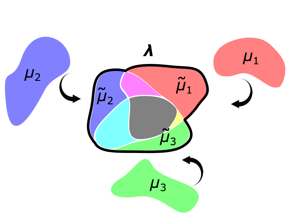
where we use the notation Bμ∗B_{\mu}^{*} for future reference; see Figure 1 for a pictorial explanation.
Refer to caption
Figure 1. Picture for (2.8). μi\mu_{i}’s are first moved to μ~i\widetilde{\mu}_{i}’s and λ\lambda is chosen to cover all μ~i\widetilde{\mu}_{i}’s: it is the smallest positive measure which is larger than all μ~i\widetilde{\mu}_{i}’s.
Remark 2.6.

It is straightforward to see from (2.7) that Bμ∗B_{\mu}^{*} is 11-homogeneous in μ\mu. That is, if a>0a>0, then Ba​μ∗=a​Bμ∗B^{*}_{a\mu}=aB^{*}_{\mu}.

2.1. The MOT problem

2.1.1. General MOT problems

Before providing the details of our MOT problem (1.2), it is worth introducing the generic MOT problem first. Let 𝒮1,…,𝒮K\mathcal{S}_{1},\dots,\mathcal{S}_{K} be fixed spaces and let 𝐜:𝒮1×⋯×𝒮K→ℝ∪{+∞,−∞}\mathbf{c}:\mathcal{S}_{1}\times\dots\times\mathcal{S}_{K}\to\mathbb{R}\cup\{+\infty,-\infty\} be a cost function. For each 1≤k≤K1\leq k\leq K, let νk∈𝒫⁡(𝒮k)\nu_{k}\in\mathcal{P}(\mathcal{S}_{k}) be a Borel probability measure. The MOT problem associated to the cost function 𝐜\mathbf{c} and the measures ν1,…,νK\nu_{1},\dots,\nu_{K} is the following (possibly infinite dimensional) linear optimization problem with KK-marginal constraints:

infπ∈Π⁡(ν1,…,νK)∫𝒮1×⋯×𝒮K𝐜⁡(ξ1,…,ξK)​𝑑π​(ξ1,…,ξK),\inf_{\pi\in\Pi(\nu_{1},\dots,\nu_{K})}\int_{\mathcal{S}_{1}\times\dots\times\mathcal{S}_{K}}\mathbf{c}(\xi_{1},\dots,\xi_{K})d\pi(\xi_{1},\dots,\xi_{K}),

where

Π⁡(ν1,…,νK):={π∈𝒫⁡(𝒮1×⋯×𝒮K), s.t.,  for every ​i, i-th marginal of ​π=νi}.\Pi(\nu_{1},\dots,\nu_{K}):=\{\pi\in\mathcal{P}(\mathcal{S}_{1}\times\dots\times\mathcal{S}_{K}),\text{ s.t., }\text{ for every }i,\text{ $i$-th marginal of }\pi=\nu_{i}\}.

MOTs are generalizations of the standard (two marginals) optimal transport (OT) problems and their duals take the form:

(2.9) supϕ∈Φ{∑j=1K∫𝒮jϕj​(ξj)​d​νj​(ξj)},\sup_{\phi\in\Phi}\left\{\sum_{j=1}^{K}\int_{\mathcal{S}_{j}}\phi_{j}(\xi_{j})d\nu_{j}(\xi_{j})\right\},

where Φ\Phi is the set of all ϕ=(ϕ1,…,ϕK)∈∏j=1KL1​(νj)\phi=(\phi_{1},\dots,\phi_{K})\in\prod_{j=1}^{K}L^{1}(\nu_{j}) such that

∑j=1Kϕj​(ξj)≤𝐜⁡(ξ1,…,ξK),∀(ξ1,…,ξK)∈𝒮1×⋯×𝒮K.\sum_{j=1}^{K}\phi_{j}(\xi_{j})\leq\mathbf{c}(\xi_{1},\dots,\xi_{K}),\quad\forall(\xi_{1},\dots,\xi_{K})\in\mathcal{S}_{1}\times\dots\times\mathcal{S}_{K}.

One of the most popular examples of MOT problems is connected to the Wasserstein Barycenter problem over 𝒫⁡(𝒳)\mathcal{P}(\mathcal{X}); see [Eke05, CMN10, AC11]. Let c:𝒳×𝒳→ℝ∪{+∞,−∞}c:\mathcal{X}\times\mathcal{X}\to\mathbb{R}\cup\{+\infty,-\infty\} be a fixed pairwise cost function. In the Wasserstein barycenter problem the goal is to find a solution ν∗\nu^{*} to the problem

infν′∑i∈[K]C⁡(ν′,νi)where ​C​(ν,νi):=infπ∈Π⁡(ν,νi)∫𝒳×𝒳c⁡(x′,x)​𝑑π​(x′,x).\inf_{\nu^{\prime}}\sum_{i\in[K]}C(\nu^{\prime},\nu_{i})\quad\text{where }C(\nu,\nu_{i}):=\inf_{\pi\in\Pi(\nu,\nu_{i})}\int_{\mathcal{X}\times\mathcal{X}}c(x^{\prime},x)d\pi(x^{\prime},x).

Such ν∗\nu^{*} can be interpreted as an “average” or barycenter of the input measures ν1,…,νK\nu_{1},\dots,\nu_{K} relative to the cost CC. It can then be showed that the above Wasserstein barycenter problem is equivalent to solving the following MOT problem

infπ∈Π⁡(ν1,…,νK)∫𝒳K𝐜⁡(x1,…,xK)​𝑑π​(x1,…,xK),\inf_{\pi\in\Pi(\nu_{1},\dots,\nu_{K})}\int_{\mathcal{X}^{K}}\mathbf{c}(x_{1},\dots,x_{K})d\pi(x_{1},\dots,x_{K}),

where

𝐜⁡(x1,…,xK):=infx′∈𝒳∑i∈[K]c⁡(x′,xi).\mathbf{c}(x_{1},\dots,x_{K}):=\inf_{x^{\prime}\in\mathcal{X}}\sum_{i\in[K]}c(x^{\prime},x_{i}).

Indeed, let π∗\pi^{*} be a minimizer of the above MOT problem. Defining ν∗=T#​π\nu^{*}=T_{\#}\pi, where T(x1,…,xK):=argminx′∑i∈[K]c(x′,xi)T(x_{1},\dots,x_{K}):=\argmin_{x^{\prime}}\sum_{i\in[K]}c(x^{\prime},x_{i}), i.e., defining ν∗\nu^{*} as the pushforward measure of π∗\pi^{*} with respect to the barycenter mapping TT, one can recover a solution to the original barycenter problem. Conversely, one can use a Wasserstein barycenter ν∗\nu^{*} and couplings πi\pi_{i} realizing the costs C⁡(ν∗,νi)C(\nu^{*},\nu_{i}) to build a solution to the MOT problem; see more details in [AC11].

2.1.2. From adversarial robustness to MOT

Now we are ready to state problem (1.2) precisely. For this, we will need to modify the space 𝒵\mathcal{Z} and in particular add an extra element to it that will be denoted by the symbol   \roundcap \cbezier (-1.5,-1.5)(-1,-1)(-1,-.5)(-1,0)\Line(-1,0)(-1,.5)\cbezier(1.5,-1.5)(1,-1)(1,-.5)(1,0)\Line(1,0)(1,.5)\cbezier(-1,.5)(-1,2)(1,2)(1,.5)\cbezier(-1.5,-1.5)(-1.1,-1.1)(-.7,-1.9)(-.3,-1.5)  \mathord{\mathchoice{\vrule width=0.0pt,height=0.0pt,depth=1.50002pt\picture(3.2,2.6)(-1.6,-1.0)\roundcap\cbezier(-1.5,-1.5)(-1,-1)(-1,-.5)(-1,0)\Line(-1,0)(-1,.5)\cbezier(1.5,-1.5)(1,-1)(1,-.5)(1,0)\Line(1,0)(1,.5)\cbezier(-1,.5)(-1,2)(1,2)(1,.5)\cbezier(-1.5,-1.5)(-1.1,-1.1)(-.7,-1.9)(-.3,-1.5)\qbezier{}{-0.3}{-1.5}{0}{-1.2}{0.3}{-1.5}\cbezier(1.5,-1.5)(1.1,-1.1)(.7,-1.9)(.3,-1.5)\put(-0.4,0.7){\circle*{0.4}}\put(0.4,0.7){\circle*{0.4}}\endpicture}{\vrule width=0.0pt,height=0.0pt,depth=1.50002pt\picture(3.2,2.6)(-1.6,-1.0)\roundcap\cbezier(-1.5,-1.5)(-1,-1)(-1,-.5)(-1,0)\Line(-1,0)(-1,.5)\cbezier(1.5,-1.5)(1,-1)(1,-.5)(1,0)\Line(1,0)(1,.5)\cbezier(-1,.5)(-1,2)(1,2)(1,.5)\cbezier(-1.5,-1.5)(-1.1,-1.1)(-.7,-1.9)(-.3,-1.5)\qbezier{}{-0.3}{-1.5}{0}{-1.2}{0.3}{-1.5}\cbezier(1.5,-1.5)(1.1,-1.1)(.7,-1.9)(.3,-1.5)\put(-0.4,0.7){\circle*{0.4}}\put(0.4,0.7){\circle*{0.4}}\endpicture}{\vrule width=0.0pt,height=0.0pt,depth=1.50002pt\picture(3.2,2.6)(-1.6,-1.0)\roundcap\cbezier(-1.5,-1.5)(-1,-1)(-1,-.5)(-1,0)\Line(-1,0)(-1,.5)\cbezier(1.5,-1.5)(1,-1)(1,-.5)(1,0)\Line(1,0)(1,.5)\cbezier(-1,.5)(-1,2)(1,2)(1,.5)\cbezier(-1.5,-1.5)(-1.1,-1.1)(-.7,-1.9)(-.3,-1.5)\qbezier{}{-0.3}{-1.5}{0}{-1.2}{0.3}{-1.5}\cbezier(1.5,-1.5)(1.1,-1.1)(.7,-1.9)(.3,-1.5)\put(-0.4,0.7){\circle*{0.4}}\put(0.4,0.7){\circle*{0.4}}\endpicture}{\vrule width=0.0pt,height=0.0pt,depth=1.50002pt\picture(3.2,2.6)(-1.6,-1.0)\roundcap\cbezier(-1.5,-1.5)(-1,-1)(-1,-.5)(-1,0)\Line(-1,0)(-1,.5)\cbezier(1.5,-1.5)(1,-1)(1,-.5)(1,0)\Line(1,0)(1,.5)\cbezier(-1,.5)(-1,2)(1,2)(1,.5)\cbezier(-1.5,-1.5)(-1.1,-1.1)(-.7,-1.9)(-.3,-1.5)\qbezier{}{-0.3}{-1.5}{0}{-1.2}{0.3}{-1.5}\cbezier(1.5,-1.5)(1.1,-1.1)(.7,-1.9)(.3,-1.5)\put(-0.4,0.7){\circle*{0.4}}\put(0.4,0.7){\circle*{0.4}}\endpicture}}. The marginals of the couplings in the desired MOT problem will be probability measures over the set 𝒵∗:=𝒵∪{  \roundcap \cbezier (-1.5,-1.5)(-1,-1)(-1,-.5)(-1,0)\Line(-1,0)(-1,.5)\cbezier(1.5,-1.5)(1,-1)(1,-.5)(1,0)\Line(1,0)(1,.5)\cbezier(-1,.5)(-1,2)(1,2)(1,.5)\cbezier(-1.5,-1.5)(-1.1,-1.1)(-.7,-1.9)(-.3,-1.5)  }\mathcal{Z}_{*}:=\mathcal{Z}\cup\{\mathord{\mathchoice{\vrule width=0.0pt,height=0.0pt,depth=1.50002pt\picture(3.2,2.6)(-1.6,-1.0)\roundcap\cbezier(-1.5,-1.5)(-1,-1)(-1,-.5)(-1,0)\Line(-1,0)(-1,.5)\cbezier(1.5,-1.5)(1,-1)(1,-.5)(1,0)\Line(1,0)(1,.5)\cbezier(-1,.5)(-1,2)(1,2)(1,.5)\cbezier(-1.5,-1.5)(-1.1,-1.1)(-.7,-1.9)(-.3,-1.5)\qbezier{}{-0.3}{-1.5}{0}{-1.2}{0.3}{-1.5}\cbezier(1.5,-1.5)(1.1,-1.1)(.7,-1.9)(.3,-1.5)\put(-0.4,0.7){\circle*{0.4}}\put(0.4,0.7){\circle*{0.4}}\endpicture}{\vrule width=0.0pt,height=0.0pt,depth=1.50002pt\picture(3.2,2.6)(-1.6,-1.0)\roundcap\cbezier(-1.5,-1.5)(-1,-1)(-1,-.5)(-1,0)\Line(-1,0)(-1,.5)\cbezier(1.5,-1.5)(1,-1)(1,-.5)(1,0)\Line(1,0)(1,.5)\cbezier(-1,.5)(-1,2)(1,2)(1,.5)\cbezier(-1.5,-1.5)(-1.1,-1.1)(-.7,-1.9)(-.3,-1.5)\qbezier{}{-0.3}{-1.5}{0}{-1.2}{0.3}{-1.5}\cbezier(1.5,-1.5)(1.1,-1.1)(.7,-1.9)(.3,-1.5)\put(-0.4,0.7){\circle*{0.4}}\put(0.4,0.7){\circle*{0.4}}\endpicture}{\vrule width=0.0pt,height=0.0pt,depth=1.50002pt\picture(3.2,2.6)(-1.6,-1.0)\roundcap\cbezier(-1.5,-1.5)(-1,-1)(-1,-.5)(-1,0)\Line(-1,0)(-1,.5)\cbezier(1.5,-1.5)(1,-1)(1,-.5)(1,0)\Line(1,0)(1,.5)\cbezier(-1,.5)(-1,2)(1,2)(1,.5)\cbezier(-1.5,-1.5)(-1.1,-1.1)(-.7,-1.9)(-.3,-1.5)\qbezier{}{-0.3}{-1.5}{0}{-1.2}{0.3}{-1.5}\cbezier(1.5,-1.5)(1.1,-1.1)(.7,-1.9)(.3,-1.5)\put(-0.4,0.7){\circle*{0.4}}\put(0.4,0.7){\circle*{0.4}}\endpicture}{\vrule width=0.0pt,height=0.0pt,depth=1.50002pt\picture(3.2,2.6)(-1.6,-1.0)\roundcap\cbezier(-1.5,-1.5)(-1,-1)(-1,-.5)(-1,0)\Line(-1,0)(-1,.5)\cbezier(1.5,-1.5)(1,-1)(1,-.5)(1,0)\Line(1,0)(1,.5)\cbezier(-1,.5)(-1,2)(1,2)(1,.5)\cbezier(-1.5,-1.5)(-1.1,-1.1)(-.7,-1.9)(-.3,-1.5)\qbezier{}{-0.3}{-1.5}{0}{-1.2}{0.3}{-1.5}\cbezier(1.5,-1.5)(1.1,-1.1)(.7,-1.9)(.3,-1.5)\put(-0.4,0.7){\circle*{0.4}}\put(0.4,0.7){\circle*{0.4}}\endpicture}}\}. More precisely, letting PiP_{i} represent the projection onto the ii-th coordinate, we consider the set:

(2.10) ΠK(μ):={π∈𝒫(𝒵∗K):Pi​♯π=12​μ​(𝒵)μ(⋅∩𝒵)+12δ  \roundcap \cbezier (-1.5,-1.5)(-1,-1)(-1,-.5)(-1,0)\Line(-1,0)(-1,.5)\cbezier(1.5,-1.5)(1,-1)(1,-.5)(1,0)\Line(1,0)(1,.5)\cbezier(-1,.5)(-1,2)(1,2)(1,.5)\cbezier(-1.5,-1.5)(-1.1,-1.1)(-.7,-1.9)(-.3,-1.5)   for all i∈[K]}.\Pi_{K}(\mu):=\left\{\pi\in\mathcal{P}(\mathcal{Z}_{*}^{K})\>:\>P_{i\sharp}\pi=\frac{1}{2\mu(\mathcal{Z})}\mu(\cdot\cap\mathcal{Z})+\frac{1}{2}\delta_{\mathord{\mathchoice{\vrule width=0.0pt,height=0.0pt,depth=1.22917pt\picture(3.2,2.6)(-1.6,-1.0)\roundcap\cbezier(-1.5,-1.5)(-1,-1)(-1,-.5)(-1,0)\Line(-1,0)(-1,.5)\cbezier(1.5,-1.5)(1,-1)(1,-.5)(1,0)\Line(1,0)(1,.5)\cbezier(-1,.5)(-1,2)(1,2)(1,.5)\cbezier(-1.5,-1.5)(-1.1,-1.1)(-.7,-1.9)(-.3,-1.5)\qbezier{}{-0.3}{-1.5}{0}{-1.2}{0.3}{-1.5}\cbezier(1.5,-1.5)(1.1,-1.1)(.7,-1.9)(.3,-1.5)\put(-0.4,0.7){\circle*{0.4}}\put(0.4,0.7){\circle*{0.4}}\endpicture}{\vrule width=0.0pt,height=0.0pt,depth=1.22917pt\picture(3.2,2.6)(-1.6,-1.0)\roundcap\cbezier(-1.5,-1.5)(-1,-1)(-1,-.5)(-1,0)\Line(-1,0)(-1,.5)\cbezier(1.5,-1.5)(1,-1)(1,-.5)(1,0)\Line(1,0)(1,.5)\cbezier(-1,.5)(-1,2)(1,2)(1,.5)\cbezier(-1.5,-1.5)(-1.1,-1.1)(-.7,-1.9)(-.3,-1.5)\qbezier{}{-0.3}{-1.5}{0}{-1.2}{0.3}{-1.5}\cbezier(1.5,-1.5)(1.1,-1.1)(.7,-1.9)(.3,-1.5)\put(-0.4,0.7){\circle*{0.4}}\put(0.4,0.7){\circle*{0.4}}\endpicture}{\vrule width=0.0pt,height=0.0pt,depth=1.22917pt\picture(3.2,2.6)(-1.6,-1.0)\roundcap\cbezier(-1.5,-1.5)(-1,-1)(-1,-.5)(-1,0)\Line(-1,0)(-1,.5)\cbezier(1.5,-1.5)(1,-1)(1,-.5)(1,0)\Line(1,0)(1,.5)\cbezier(-1,.5)(-1,2)(1,2)(1,.5)\cbezier(-1.5,-1.5)(-1.1,-1.1)(-.7,-1.9)(-.3,-1.5)\qbezier{}{-0.3}{-1.5}{0}{-1.2}{0.3}{-1.5}\cbezier(1.5,-1.5)(1.1,-1.1)(.7,-1.9)(.3,-1.5)\put(-0.4,0.7){\circle*{0.4}}\put(0.4,0.7){\circle*{0.4}}\endpicture}{\vrule width=0.0pt,height=0.0pt,depth=1.22917pt\picture(3.2,2.6)(-1.6,-1.0)\roundcap\cbezier(-1.5,-1.5)(-1,-1)(-1,-.5)(-1,0)\Line(-1,0)(-1,.5)\cbezier(1.5,-1.5)(1,-1)(1,-.5)(1,0)\Line(1,0)(1,.5)\cbezier(-1,.5)(-1,2)(1,2)(1,.5)\cbezier(-1.5,-1.5)(-1.1,-1.1)(-.7,-1.9)(-.3,-1.5)\qbezier{}{-0.3}{-1.5}{0}{-1.2}{0.3}{-1.5}\cbezier(1.5,-1.5)(1.1,-1.1)(.7,-1.9)(.3,-1.5)\put(-0.4,0.7){\circle*{0.4}}\put(0.4,0.7){\circle*{0.4}}\endpicture}}}\text{ for all }i\in[K]\right\}.

Notice that in this set all KK marginals are the same. Dividing by the factor 12​μ​(𝒵)\frac{1}{2\mu(\mathcal{Z})}, the set ΠK​(μ)\Pi_{K}(\mu) is made to be consistent with the literature on multimarginal optimal transport, where sets of couplings are typically assumed to be probability measures.

Let us now discuss the cost function for the desired MOT problem. For a given tuple (z1,…,zK)(z_{1},\dots,z_{K}) in 𝒵∗K\mathcal{Z}_{*}^{K}, often denoted by z→\vec{z} in the sequel for convenience, we define

(2.11) 𝐜⁡(z1,…,zK):=Bμ^z→∗,\mathbf{c}(z_{1},\dots,z_{K}):=B^{*}_{\widehat{\mu}_{\vec{z}}},

where μ^z→\widehat{\mu}_{\vec{z}} is the positive measure (not necessarily a probability measure) defined as:

μ^z→:=1K​∑l​ s.t. ​zl≠  \roundcap \cbezier (-1.5,-1.5)(-1,-1)(-1,-.5)(-1,0)\Line(-1,0)(-1,.5)\cbezier(1.5,-1.5)(1,-1)(1,-.5)(1,0)\Line(1,0)(1,.5)\cbezier(-1,.5)(-1,2)(1,2)(1,.5)\cbezier(-1.5,-1.5)(-1.1,-1.1)(-.7,-1.9)(-.3,-1.5)  Kδzl.\widehat{\mu}_{\vec{z}}:=\frac{1}{K}\sum_{l\text{ s.t. }z_{l}\not=\mathord{\mathchoice{\vrule width=0.0pt,height=0.0pt,depth=1.22917pt\picture(3.2,2.6)(-1.6,-1.0)\roundcap\cbezier(-1.5,-1.5)(-1,-1)(-1,-.5)(-1,0)\Line(-1,0)(-1,.5)\cbezier(1.5,-1.5)(1,-1)(1,-.5)(1,0)\Line(1,0)(1,.5)\cbezier(-1,.5)(-1,2)(1,2)(1,.5)\cbezier(-1.5,-1.5)(-1.1,-1.1)(-.7,-1.9)(-.3,-1.5)\qbezier{}{-0.3}{-1.5}{0}{-1.2}{0.3}{-1.5}\cbezier(1.5,-1.5)(1.1,-1.1)(.7,-1.9)(.3,-1.5)\put(-0.4,0.7){\circle*{0.4}}\put(0.4,0.7){\circle*{0.4}}\endpicture}{\vrule width=0.0pt,height=0.0pt,depth=1.22917pt\picture(3.2,2.6)(-1.6,-1.0)\roundcap\cbezier(-1.5,-1.5)(-1,-1)(-1,-.5)(-1,0)\Line(-1,0)(-1,.5)\cbezier(1.5,-1.5)(1,-1)(1,-.5)(1,0)\Line(1,0)(1,.5)\cbezier(-1,.5)(-1,2)(1,2)(1,.5)\cbezier(-1.5,-1.5)(-1.1,-1.1)(-.7,-1.9)(-.3,-1.5)\qbezier{}{-0.3}{-1.5}{0}{-1.2}{0.3}{-1.5}\cbezier(1.5,-1.5)(1.1,-1.1)(.7,-1.9)(.3,-1.5)\put(-0.4,0.7){\circle*{0.4}}\put(0.4,0.7){\circle*{0.4}}\endpicture}{\vrule width=0.0pt,height=0.0pt,depth=1.22917pt\picture(3.2,2.6)(-1.6,-1.0)\roundcap\cbezier(-1.5,-1.5)(-1,-1)(-1,-.5)(-1,0)\Line(-1,0)(-1,.5)\cbezier(1.5,-1.5)(1,-1)(1,-.5)(1,0)\Line(1,0)(1,.5)\cbezier(-1,.5)(-1,2)(1,2)(1,.5)\cbezier(-1.5,-1.5)(-1.1,-1.1)(-.7,-1.9)(-.3,-1.5)\qbezier{}{-0.3}{-1.5}{0}{-1.2}{0.3}{-1.5}\cbezier(1.5,-1.5)(1.1,-1.1)(.7,-1.9)(.3,-1.5)\put(-0.4,0.7){\circle*{0.4}}\put(0.4,0.7){\circle*{0.4}}\endpicture}{\vrule width=0.0pt,height=0.0pt,depth=1.22917pt\picture(3.2,2.6)(-1.6,-1.0)\roundcap\cbezier(-1.5,-1.5)(-1,-1)(-1,-.5)(-1,0)\Line(-1,0)(-1,.5)\cbezier(1.5,-1.5)(1,-1)(1,-.5)(1,0)\Line(1,0)(1,.5)\cbezier(-1,.5)(-1,2)(1,2)(1,.5)\cbezier(-1.5,-1.5)(-1.1,-1.1)(-.7,-1.9)(-.3,-1.5)\qbezier{}{-0.3}{-1.5}{0}{-1.2}{0.3}{-1.5}\cbezier(1.5,-1.5)(1.1,-1.1)(.7,-1.9)(.3,-1.5)\put(-0.4,0.7){\circle*{0.4}}\put(0.4,0.7){\circle*{0.4}}\endpicture}}}^{K}\delta_{z_{l}}.

Recall that Bμ^z→∗B^{*}_{\widehat{\mu}_{\vec{z}}} is equal to (2.8) (alternatively, equal to (2.7)) when μ\mu is equal to μ^z→{\widehat{\mu}_{\vec{z}}}. In this sense, 𝐜⁡(z1,…,zK)\mathbf{c}(z_{1},\dots,z_{K}) of (2.11) is the value of the generalized barycenter problem given μ^z→\widehat{\mu}_{\vec{z}} as the data distribution, or local generalized barycenter problem.

Remark 2.7.

Notice that μ^z→\widehat{\mu}_{\vec{z}} is a probability measure if and only if no element in the tuple z→\vec{z} is   \roundcap \cbezier (-1.5,-1.5)(-1,-1)(-1,-.5)(-1,0)\Line(-1,0)(-1,.5)\cbezier(1.5,-1.5)(1,-1)(1,-.5)(1,0)\Line(1,0)(1,.5)\cbezier(-1,.5)(-1,2)(1,2)(1,.5)\cbezier(-1.5,-1.5)(-1.1,-1.1)(-.7,-1.9)(-.3,-1.5)  \mathord{\mathchoice{\vrule width=0.0pt,height=0.0pt,depth=1.50002pt\picture(3.2,2.6)(-1.6,-1.0)\roundcap\cbezier(-1.5,-1.5)(-1,-1)(-1,-.5)(-1,0)\Line(-1,0)(-1,.5)\cbezier(1.5,-1.5)(1,-1)(1,-.5)(1,0)\Line(1,0)(1,.5)\cbezier(-1,.5)(-1,2)(1,2)(1,.5)\cbezier(-1.5,-1.5)(-1.1,-1.1)(-.7,-1.9)(-.3,-1.5)\qbezier{}{-0.3}{-1.5}{0}{-1.2}{0.3}{-1.5}\cbezier(1.5,-1.5)(1.1,-1.1)(.7,-1.9)(.3,-1.5)\put(-0.4,0.7){\circle*{0.4}}\put(0.4,0.7){\circle*{0.4}}\endpicture}{\vrule width=0.0pt,height=0.0pt,depth=1.50002pt\picture(3.2,2.6)(-1.6,-1.0)\roundcap\cbezier(-1.5,-1.5)(-1,-1)(-1,-.5)(-1,0)\Line(-1,0)(-1,.5)\cbezier(1.5,-1.5)(1,-1)(1,-.5)(1,0)\Line(1,0)(1,.5)\cbezier(-1,.5)(-1,2)(1,2)(1,.5)\cbezier(-1.5,-1.5)(-1.1,-1.1)(-.7,-1.9)(-.3,-1.5)\qbezier{}{-0.3}{-1.5}{0}{-1.2}{0.3}{-1.5}\cbezier(1.5,-1.5)(1.1,-1.1)(.7,-1.9)(.3,-1.5)\put(-0.4,0.7){\circle*{0.4}}\put(0.4,0.7){\circle*{0.4}}\endpicture}{\vrule width=0.0pt,height=0.0pt,depth=1.50002pt\picture(3.2,2.6)(-1.6,-1.0)\roundcap\cbezier(-1.5,-1.5)(-1,-1)(-1,-.5)(-1,0)\Line(-1,0)(-1,.5)\cbezier(1.5,-1.5)(1,-1)(1,-.5)(1,0)\Line(1,0)(1,.5)\cbezier(-1,.5)(-1,2)(1,2)(1,.5)\cbezier(-1.5,-1.5)(-1.1,-1.1)(-.7,-1.9)(-.3,-1.5)\qbezier{}{-0.3}{-1.5}{0}{-1.2}{0.3}{-1.5}\cbezier(1.5,-1.5)(1.1,-1.1)(.7,-1.9)(.3,-1.5)\put(-0.4,0.7){\circle*{0.4}}\put(0.4,0.7){\circle*{0.4}}\endpicture}{\vrule width=0.0pt,height=0.0pt,depth=1.50002pt\picture(3.2,2.6)(-1.6,-1.0)\roundcap\cbezier(-1.5,-1.5)(-1,-1)(-1,-.5)(-1,0)\Line(-1,0)(-1,.5)\cbezier(1.5,-1.5)(1,-1)(1,-.5)(1,0)\Line(1,0)(1,.5)\cbezier(-1,.5)(-1,2)(1,2)(1,.5)\cbezier(-1.5,-1.5)(-1.1,-1.1)(-.7,-1.9)(-.3,-1.5)\qbezier{}{-0.3}{-1.5}{0}{-1.2}{0.3}{-1.5}\cbezier(1.5,-1.5)(1.1,-1.1)(.7,-1.9)(.3,-1.5)\put(-0.4,0.7){\circle*{0.4}}\put(0.4,0.7){\circle*{0.4}}\endpicture}}.

Following the literature of MOT, the dual of our MOT problem can be written as

(2.12) supϕ∈Φ{∑j=1K∫𝒳×[K]ϕj​(zj)​12​μ​(𝒵)​𝑑μ​(zj)+12​∑j=1Kϕj​(  \roundcap \cbezier (-1.5,-1.5)(-1,-1)(-1,-.5)(-1,0)\Line(-1,0)(-1,.5)\cbezier(1.5,-1.5)(1,-1)(1,-.5)(1,0)\Line(1,0)(1,.5)\cbezier(-1,.5)(-1,2)(1,2)(1,.5)\cbezier(-1.5,-1.5)(-1.1,-1.1)(-.7,-1.9)(-.3,-1.5)  )},\sup_{\phi\in\Phi}\left\{\sum_{j=1}^{K}\int_{\mathcal{X}\times[K]}\phi_{j}(z_{j})\frac{1}{2\mu(\mathcal{Z})}d\mu(z_{j})+\frac{1}{2}\sum_{j=1}^{K}\phi_{j}(\mathord{\mathchoice{\vrule width=0.0pt,height=0.0pt,depth=1.50002pt\picture(3.2,2.6)(-1.6,-1.0)\roundcap\cbezier(-1.5,-1.5)(-1,-1)(-1,-.5)(-1,0)\Line(-1,0)(-1,.5)\cbezier(1.5,-1.5)(1,-1)(1,-.5)(1,0)\Line(1,0)(1,.5)\cbezier(-1,.5)(-1,2)(1,2)(1,.5)\cbezier(-1.5,-1.5)(-1.1,-1.1)(-.7,-1.9)(-.3,-1.5)\qbezier{}{-0.3}{-1.5}{0}{-1.2}{0.3}{-1.5}\cbezier(1.5,-1.5)(1.1,-1.1)(.7,-1.9)(.3,-1.5)\put(-0.4,0.7){\circle*{0.4}}\put(0.4,0.7){\circle*{0.4}}\endpicture}{\vrule width=0.0pt,height=0.0pt,depth=1.50002pt\picture(3.2,2.6)(-1.6,-1.0)\roundcap\cbezier(-1.5,-1.5)(-1,-1)(-1,-.5)(-1,0)\Line(-1,0)(-1,.5)\cbezier(1.5,-1.5)(1,-1)(1,-.5)(1,0)\Line(1,0)(1,.5)\cbezier(-1,.5)(-1,2)(1,2)(1,.5)\cbezier(-1.5,-1.5)(-1.1,-1.1)(-.7,-1.9)(-.3,-1.5)\qbezier{}{-0.3}{-1.5}{0}{-1.2}{0.3}{-1.5}\cbezier(1.5,-1.5)(1.1,-1.1)(.7,-1.9)(.3,-1.5)\put(-0.4,0.7){\circle*{0.4}}\put(0.4,0.7){\circle*{0.4}}\endpicture}{\vrule width=0.0pt,height=0.0pt,depth=1.50002pt\picture(3.2,2.6)(-1.6,-1.0)\roundcap\cbezier(-1.5,-1.5)(-1,-1)(-1,-.5)(-1,0)\Line(-1,0)(-1,.5)\cbezier(1.5,-1.5)(1,-1)(1,-.5)(1,0)\Line(1,0)(1,.5)\cbezier(-1,.5)(-1,2)(1,2)(1,.5)\cbezier(-1.5,-1.5)(-1.1,-1.1)(-.7,-1.9)(-.3,-1.5)\qbezier{}{-0.3}{-1.5}{0}{-1.2}{0.3}{-1.5}\cbezier(1.5,-1.5)(1.1,-1.1)(.7,-1.9)(.3,-1.5)\put(-0.4,0.7){\circle*{0.4}}\put(0.4,0.7){\circle*{0.4}}\endpicture}{\vrule width=0.0pt,height=0.0pt,depth=1.50002pt\picture(3.2,2.6)(-1.6,-1.0)\roundcap\cbezier(-1.5,-1.5)(-1,-1)(-1,-.5)(-1,0)\Line(-1,0)(-1,.5)\cbezier(1.5,-1.5)(1,-1)(1,-.5)(1,0)\Line(1,0)(1,.5)\cbezier(-1,.5)(-1,2)(1,2)(1,.5)\cbezier(-1.5,-1.5)(-1.1,-1.1)(-.7,-1.9)(-.3,-1.5)\qbezier{}{-0.3}{-1.5}{0}{-1.2}{0.3}{-1.5}\cbezier(1.5,-1.5)(1.1,-1.1)(.7,-1.9)(.3,-1.5)\put(-0.4,0.7){\circle*{0.4}}\put(0.4,0.7){\circle*{0.4}}\endpicture}})\right\},

where

(2.13) Φ:={ϕ=(ϕ1,…,ϕK)∈∏j=1KL1(12​μ​(𝒵)μ+12δ  \roundcap \cbezier (-1.5,-1.5)(-1,-1)(-1,-.5)(-1,0)\Line(-1,0)(-1,.5)\cbezier(1.5,-1.5)(1,-1)(1,-.5)(1,0)\Line(1,0)(1,.5)\cbezier(-1,.5)(-1,2)(1,2)(1,.5)\cbezier(-1.5,-1.5)(-1.1,-1.1)(-.7,-1.9)(-.3,-1.5)  ):∑j=1Kϕj(zj)≤Bμ^z→∗,∀z→∈𝒵∗K}.\Phi:=\left\{\phi=(\phi_{1},\dots,\phi_{K})\in\prod_{j=1}^{K}L^{1}\big(\frac{1}{2\mu(\mathcal{Z})}\mu+\frac{1}{2}\delta_{\mathord{\mathchoice{\vrule width=0.0pt,height=0.0pt,depth=1.22917pt\picture(3.2,2.6)(-1.6,-1.0)\roundcap\cbezier(-1.5,-1.5)(-1,-1)(-1,-.5)(-1,0)\Line(-1,0)(-1,.5)\cbezier(1.5,-1.5)(1,-1)(1,-.5)(1,0)\Line(1,0)(1,.5)\cbezier(-1,.5)(-1,2)(1,2)(1,.5)\cbezier(-1.5,-1.5)(-1.1,-1.1)(-.7,-1.9)(-.3,-1.5)\qbezier{}{-0.3}{-1.5}{0}{-1.2}{0.3}{-1.5}\cbezier(1.5,-1.5)(1.1,-1.1)(.7,-1.9)(.3,-1.5)\put(-0.4,0.7){\circle*{0.4}}\put(0.4,0.7){\circle*{0.4}}\endpicture}{\vrule width=0.0pt,height=0.0pt,depth=1.22917pt\picture(3.2,2.6)(-1.6,-1.0)\roundcap\cbezier(-1.5,-1.5)(-1,-1)(-1,-.5)(-1,0)\Line(-1,0)(-1,.5)\cbezier(1.5,-1.5)(1,-1)(1,-.5)(1,0)\Line(1,0)(1,.5)\cbezier(-1,.5)(-1,2)(1,2)(1,.5)\cbezier(-1.5,-1.5)(-1.1,-1.1)(-.7,-1.9)(-.3,-1.5)\qbezier{}{-0.3}{-1.5}{0}{-1.2}{0.3}{-1.5}\cbezier(1.5,-1.5)(1.1,-1.1)(.7,-1.9)(.3,-1.5)\put(-0.4,0.7){\circle*{0.4}}\put(0.4,0.7){\circle*{0.4}}\endpicture}{\vrule width=0.0pt,height=0.0pt,depth=1.22917pt\picture(3.2,2.6)(-1.6,-1.0)\roundcap\cbezier(-1.5,-1.5)(-1,-1)(-1,-.5)(-1,0)\Line(-1,0)(-1,.5)\cbezier(1.5,-1.5)(1,-1)(1,-.5)(1,0)\Line(1,0)(1,.5)\cbezier(-1,.5)(-1,2)(1,2)(1,.5)\cbezier(-1.5,-1.5)(-1.1,-1.1)(-.7,-1.9)(-.3,-1.5)\qbezier{}{-0.3}{-1.5}{0}{-1.2}{0.3}{-1.5}\cbezier(1.5,-1.5)(1.1,-1.1)(.7,-1.9)(.3,-1.5)\put(-0.4,0.7){\circle*{0.4}}\put(0.4,0.7){\circle*{0.4}}\endpicture}{\vrule width=0.0pt,height=0.0pt,depth=1.22917pt\picture(3.2,2.6)(-1.6,-1.0)\roundcap\cbezier(-1.5,-1.5)(-1,-1)(-1,-.5)(-1,0)\Line(-1,0)(-1,.5)\cbezier(1.5,-1.5)(1,-1)(1,-.5)(1,0)\Line(1,0)(1,.5)\cbezier(-1,.5)(-1,2)(1,2)(1,.5)\cbezier(-1.5,-1.5)(-1.1,-1.1)(-.7,-1.9)(-.3,-1.5)\qbezier{}{-0.3}{-1.5}{0}{-1.2}{0.3}{-1.5}\cbezier(1.5,-1.5)(1.1,-1.1)(.7,-1.9)(.3,-1.5)\put(-0.4,0.7){\circle*{0.4}}\put(0.4,0.7){\circle*{0.4}}\endpicture}}}\big):\sum_{j=1}^{K}\phi_{j}(z_{j})\leq B^{*}_{\widehat{\mu}_{\vec{z}}},\quad\forall\vec{z}\in\mathcal{Z}_{*}^{K}\right\}.

We will later show that under Assumption 2.1 there is no duality gap between the MOT problem and its dual (2.12) —see Corollary 4.5.

One of the main results of the paper is the following.

Theorem 2.8.

Suppose that Assumption 2.1 holds. Let μ\mu be a finite positive measure over 𝒵\mathcal{Z}. Then (2.7) is equivalent to the MOT problem (1.2) with set of couplings ΠK​(μ)\Pi_{K}(\mu) defined as in (2.10), and cost function 𝐜\mathbf{c} defined as in (2.11). Specifically,

12​μ​(𝒵)​Bμ∗=min⁡∫π∈ΠK​(μ)⁡𝐜⁡(z1,…,zK)​𝑑π​(z1,…,zK).\frac{1}{2\mu(\mathcal{Z})}B^{*}_{\mu}=\min_{\pi\in\Pi_{K}(\mu)}\int\mathbf{c}(z_{1},\dots,z_{K})d\pi(z_{1},\dots,z_{K}).

Furthermore, (2.6)=(2.7)\eqref{def:RobustClassifPower}=\eqref{eqn:DualAdversarial}. In addition, from a solution pair (π∗,ϕ∗)(\pi^{*},\phi^{*}) for the MOT problem and its dual one can obtain a solution pair (f∗,μ~∗)(f^{*},\widetilde{\mu}^{*}) for (2.7) and its dual, i.e. problem (2.6). The pair (f∗,μ~∗)(f^{*},\widetilde{\mu}^{*}) is also a saddle point for the original adversarial problem (1.1).

One immediate consequence of Theorem 2.8 is that with the identity

Rμ∗=μ⁡(𝒵)−B~μ∗,R^{*}_{\mu}=\mu(\mathcal{Z})-\widetilde{B}^{*}_{\mu},

one can compute Rμ∗R^{*}_{\mu}, the optimal adversarial risk, by finding the optimal value of the equivalent MOT problem. To find the latter, one could attempt to use one of the off-the-shelf algorithms in computational optimal transport. Some algorithms to solve generic MOTs that have been developed recently include the ones proposed in see [BCC+15, BCN19, LHCJ22, TDGU20, HRCK21, ABA21, Car22]. Our numerical results for a subsample of MNIST and CIFAR 10, shown in Figure 6, are obtained using the algorithm discussed in [LHCJ22], also known as MOT Sinkhorn algorithm; see subsection 5.3 for more details. We want to warn the reader, however, that off-the-shelf MOT algorithms may suffer an excessive computational burden when KK goes beyond 44. For this reason, it is important to develop algorithms that exploit the structure of our MOT problem, which, as we will discuss below, has the structure of a generalized barycenter problem. An investigation on more specific algorithms is left for future work.

The proof of Theorem 2.8 is presented throughout section 4; the expression for (f∗,μ~∗)(f^{*},\widetilde{\mu}^{*}) in terms of (ϕ∗,π∗)(\phi^{*},\pi^{*}) is presented in Corollary 4.7. Given the definition of the cost function 𝐜\mathbf{c}, Theorem 2.8 states that the adversarial problem localizes to data sets consisting of KK or less equally weighted points. More precisely, the problem for the adversary reduces to first determining their actions when facing arbitrary distributions supported on KK or fewer data points, and then finding an optimal grouping for the data in order to assemble their global strategy. The ghost element,   \roundcap \cbezier (-1.5,-1.5)(-1,-1)(-1,-.5)(-1,0)\Line(-1,0)(-1,.5)\cbezier(1.5,-1.5)(1,-1)(1,-.5)(1,0)\Line(1,0)(1,.5)\cbezier(-1,.5)(-1,2)(1,2)(1,.5)\cbezier(-1.5,-1.5)(-1.1,-1.1)(-.7,-1.9)(-.3,-1.5)  \mathord{\mathchoice{\vrule width=0.0pt,height=0.0pt,depth=1.50002pt\picture(3.2,2.6)(-1.6,-1.0)\roundcap\cbezier(-1.5,-1.5)(-1,-1)(-1,-.5)(-1,0)\Line(-1,0)(-1,.5)\cbezier(1.5,-1.5)(1,-1)(1,-.5)(1,0)\Line(1,0)(1,.5)\cbezier(-1,.5)(-1,2)(1,2)(1,.5)\cbezier(-1.5,-1.5)(-1.1,-1.1)(-.7,-1.9)(-.3,-1.5)\qbezier{}{-0.3}{-1.5}{0}{-1.2}{0.3}{-1.5}\cbezier(1.5,-1.5)(1.1,-1.1)(.7,-1.9)(.3,-1.5)\put(-0.4,0.7){\circle*{0.4}}\put(0.4,0.7){\circle*{0.4}}\endpicture}{\vrule width=0.0pt,height=0.0pt,depth=1.50002pt\picture(3.2,2.6)(-1.6,-1.0)\roundcap\cbezier(-1.5,-1.5)(-1,-1)(-1,-.5)(-1,0)\Line(-1,0)(-1,.5)\cbezier(1.5,-1.5)(1,-1)(1,-.5)(1,0)\Line(1,0)(1,.5)\cbezier(-1,.5)(-1,2)(1,2)(1,.5)\cbezier(-1.5,-1.5)(-1.1,-1.1)(-.7,-1.9)(-.3,-1.5)\qbezier{}{-0.3}{-1.5}{0}{-1.2}{0.3}{-1.5}\cbezier(1.5,-1.5)(1.1,-1.1)(.7,-1.9)(.3,-1.5)\put(-0.4,0.7){\circle*{0.4}}\put(0.4,0.7){\circle*{0.4}}\endpicture}{\vrule width=0.0pt,height=0.0pt,depth=1.50002pt\picture(3.2,2.6)(-1.6,-1.0)\roundcap\cbezier(-1.5,-1.5)(-1,-1)(-1,-.5)(-1,0)\Line(-1,0)(-1,.5)\cbezier(1.5,-1.5)(1,-1)(1,-.5)(1,0)\Line(1,0)(1,.5)\cbezier(-1,.5)(-1,2)(1,2)(1,.5)\cbezier(-1.5,-1.5)(-1.1,-1.1)(-.7,-1.9)(-.3,-1.5)\qbezier{}{-0.3}{-1.5}{0}{-1.2}{0.3}{-1.5}\cbezier(1.5,-1.5)(1.1,-1.1)(.7,-1.9)(.3,-1.5)\put(-0.4,0.7){\circle*{0.4}}\put(0.4,0.7){\circle*{0.4}}\endpicture}{\vrule width=0.0pt,height=0.0pt,depth=1.50002pt\picture(3.2,2.6)(-1.6,-1.0)\roundcap\cbezier(-1.5,-1.5)(-1,-1)(-1,-.5)(-1,0)\Line(-1,0)(-1,.5)\cbezier(1.5,-1.5)(1,-1)(1,-.5)(1,0)\Line(1,0)(1,.5)\cbezier(-1,.5)(-1,2)(1,2)(1,.5)\cbezier(-1.5,-1.5)(-1.1,-1.1)(-.7,-1.9)(-.3,-1.5)\qbezier{}{-0.3}{-1.5}{0}{-1.2}{0.3}{-1.5}\cbezier(1.5,-1.5)(1.1,-1.1)(.7,-1.9)(.3,-1.5)\put(-0.4,0.7){\circle*{0.4}}\put(0.4,0.7){\circle*{0.4}}\endpicture}}, indicates when fewer than KK points are being grouped by the adversary. We highlight that it is not always (globally) optimal for the adversary to group together points from all the KK different classes whenever it is possible.

We emphasize that from the solution to the MOT and its dual, one can directly obtain an optimal adversarial attack and an optimal classification rule for the original adversarial problem. Note that problem (1.2) is a problem solved by the adversary: ideally, the adversary wants to group together points (z1,…,zK)(z_{1},\dots,z_{K}) for which there is a low classification power Bμ^z→∗B^{*}_{\widehat{\mu}_{\vec{z}}} (or alternatively large robust risk). On the other hand, the dual of (1.2) can be interpreted as a maximization problem solved by the learner. We formalize this novel connection in subsection 4.3: see Corollary 4.7.

In order to prove Theorem 2.8, we will first obtain a series of equivalent reformulations of problem (2.8) which will reveal a rich geometric structure of the adversarial problem and will facilitate the connection with the desired MOT problem. These equivalent formulations are of interest in their own right.

3. The generalized barycenter problem

We begin this section by proving that the generalized barycenter problem always has at least one solution. In the following subsections we will then discuss a series of equivalent problems to the generalized barycenter problem, their duals, and some geometric properties of their solutions.

Proposition 3.1.

Suppose that cc is a lower semicontinuous cost satisfying the property that for any compact set E⊂𝒳E\subset\mathcal{X} there exists a compact set F⊂𝒳F\subset\mathcal{X} such that for all x∈E,x′∈F,x′′∈𝒳∖Fx\in E,x^{\prime}\in F,x^{\prime\prime}\in\mathcal{X}\setminus F we have c⁡(x,x′)≤c⁡(x,x′′)c(x,x^{\prime})\leq c(x,x^{\prime\prime}). Given finite positive measures μ1,…,μK\mu_{1},\ldots,\mu_{K} and cc as above, there exists at least one solution to problem (2.8).

Remark 3.2.

If cc is a cost that satisfies Assumption 2.1, then cc satisfies the hypothesis of Proposition 3.1.

Remark 3.3.

Nearly identical arguments can be used to prove that the various reformulations of (2.8) that we will consider throughout this section have minimizers. For this reason, in what follows, we will simply assume the existence of minimizers without explicitly proving their existence.

Proof.

Using transportation plans to compute the cost C⁡(μi,μ~i)C(\mu_{i},\tilde{\mu}_{i}) in (2.8), we can rewrite the problem in the following form

infλ,π1,…,πK{λ⁡(𝒳)+∑i∈[K]∫𝒳×𝒳c⁡(x,x′)​d​πi​(x,x′)}\displaystyle\inf_{\lambda,\,\pi_{1},\ldots,\pi_{K}}\left\{\lambda(\mathcal{X})+\sum_{i\in[K]}\int_{\mathcal{X}\times\mathcal{X}}c(x,x^{\prime})d\pi_{i}(x,x^{\prime})\right\}
s.t. ​πi​(𝒳×E)≤λ⁡(E),πi​(E×𝒳)=μi​(E)​ for all ​i∈[K],∀E⊆𝒳​ Borel.\displaystyle\textup{s.t. }\pi_{i}(\mathcal{X}\times E)\leq\lambda(E),\pi_{i}(E\times\mathcal{X})=\mu_{i}(E)\text{ for all }i\in[K],\quad\forall E\subseteq{\mathcal{X}}\text{ Borel}.

Note that a feasible solution to this problem exists since we may choose λ,π1,…,πK\lambda,\pi_{1},\ldots,\pi_{K} such that λ:=∑i∈[K]μi\lambda:=\sum_{i\in[K]}\mu_{i} and for all f∈Cc​(𝒳×𝒳)f\in C_{c}(\mathcal{X}\times\mathcal{X}) ∫𝒳×𝒳f⁡(x,x′)​d​πi​(x,x′):=∫𝒳f⁡(x,x)​d​μi​(x)\int_{\mathcal{X}\times\mathcal{X}}f(x,x^{\prime})d\pi_{i}(x,x^{\prime}):=\int_{\mathcal{X}}f(x,x)d\mu_{i}(x). Also note that with these choices, the problem attains the value ∑i∈[K]μi​(𝒳)\sum_{i\in[K]}\mu_{i}(\mathcal{X}).

Let λn,π1n,…,πKn\lambda^{n},\pi_{1}^{n},\ldots,\pi_{K}^{n} be a sequence of feasible solutions such that

t\displaystyle t :=infλ,π1,…,πKλ⁡(𝒳)+∑i∈[K]∫𝒳×𝒳c⁡(x,x′)​d​πi​(x,x′)\displaystyle:=\inf_{\lambda,\pi_{1},\ldots,\pi_{K}}\lambda(\mathcal{X})+\sum_{i\in[K]}\int_{\mathcal{X}\times\mathcal{X}}c(x,x^{\prime})d\pi_{i}(x,x^{\prime})
=limn→∞λn​(𝒳)+∑i∈[K]∫𝒳×𝒳c⁡(x,x′)​d​πin​(x,x′).\displaystyle=\lim_{n\to\infty}\lambda^{n}(\mathcal{X})+\sum_{i\in[K]}\int_{\mathcal{X}\times\mathcal{X}}c(x,x^{\prime})d\pi_{i}^{n}(x,x^{\prime}).

From our work above and the nonnegativity of the transport cost, λn​(𝒳)\lambda^{n}(\mathcal{X}) is uniformly bounded by ∑i∈[K]μi​(𝒳)\sum_{i\in[K]}\mu_{i}(\mathcal{X}). Furthermore, we may assume that for any Borel set EE

∑i∈[K]∫𝒳×Ed​πin​(x,x′)≥λn​(E),\sum_{i\in[K]}\int_{\mathcal{X}\times E}d\pi_{i}^{n}(x,x^{\prime})\geq\lambda^{n}(E),

otherwise we could delete mass from λn\lambda^{n} and attain a smaller value. Given some ϵ>0\epsilon>0, let Eϵ⊂𝒳E_{\epsilon}\subset\mathcal{X} be a compact set such that ∑i∈[K]μi​(𝒳∖Eϵ)≤ϵ\sum_{i\in[K]}\mu_{i}(\mathcal{X}\setminus E_{\epsilon})\leq\epsilon. Let FϵF_{\epsilon} be a compact set such that for all x∈Eϵ,x′∈Fϵx\in E_{\epsilon},x^{\prime}\in F_{\epsilon} and x′′∈𝒳∖Fϵx^{\prime\prime}\in\mathcal{X}\setminus F_{\epsilon} we have c⁡(x,x′)≤c⁡(x,x′′)c(x,x^{\prime})\leq c(x,x^{\prime\prime}). If λn\lambda^{n} gives more than ϵ\epsilon to 𝒳∖Fϵ\mathcal{X}\setminus F_{\epsilon} then some of this mass must be transported to EϵE_{\epsilon}. Since the transportation cost would be cheaper if the excess mass was placed inside of FϵF_{\epsilon} instead of 𝒳∖Fϵ\mathcal{X}\setminus F_{\epsilon}, it follows that λn​(𝒳∖Fϵ)≤ϵ\lambda^{n}(\mathcal{X}\setminus F_{\epsilon})\leq\epsilon. Therefore, the λn\lambda^{n} are a tight family.

The tightness of λn\lambda^{n} and μ1,…,μK\mu_{1},\ldots,\mu_{K} implies that π1n,…,πKn\pi_{1}^{n},\ldots,\pi_{K}^{n} are a tight family. Therefore, we can extract a subsequence that converges weakly to a limit λ∗,π1∗,…,πK∗\lambda^{*},\pi_{1}^{*},\ldots,\pi_{K}^{*}. From the lower semicontinuity of the cost, it follows that {λ∗,π1∗,…,πK∗}\{\lambda^{*},\pi_{1}^{*},\ldots,\pi_{K}^{*}\} is a minimizer. ∎

3.1. A first MOT reformulation of (3.1) and geometric consequences

In the rest of what follows, we shall let SKS_{K} denote the power set of [K][K] except for the empty set and for every i∈[K]i\in[K] we let SK​(i)={A∈SK:i∈A}S_{K}(i)=\{A\in S_{K}:i\in A\}. We can reduce (2.8) to a more concrete problem by partitioning λ\lambda and each of μi\mu_{i}’s properly, eliminating the variables μ~i\widetilde{\mu}_{i}’s from the optimization. We start with the following observation.

Lemma 3.4.

Let u1,…,uK∈[0,1]u_{1},\dots,u_{K}\in[0,1] be such that maxi=1,…,K⁡ui=1\max_{i=1,\dots,K}u_{i}=1. Then there exists a collection of non-negative scalars {rA}A∈SK\{r_{A}\}_{A\in S_{K}} such that the following two conditions hold:

  1. (1)

    1=∑A∈SKrA1=\sum_{A\in S_{K}}r_{A}.

  2. (2)

    ui=∑A∈SK​(i)rAu_{i}=\sum_{A\in S_{K}(i)}r_{A} for all i=1,…,Ki=1,\dots,K.

Proof.

Without loss of generality we can assume that the uiu_{i} are arranged in increasing order. That is,

0≤u1≤u2≤…,≤uK=1.0\leq u_{1}\leq u_{2}\leq\dots,\leq u_{K}=1.

Let i′i^{\prime} be the first ii such that ui>0u_{i}>0. We set

r{i′,…,K}\displaystyle r_{\{i^{\prime},\dots,K\}} :=ui′\displaystyle:=u_{i^{\prime}}
r{i′+1,…,K}\displaystyle r_{\{i^{\prime}+1,\dots,K\}} :=ui′+1−ui′\displaystyle:=u_{i^{\prime}+1}-u_{i^{\prime}}
r{i′+2,…,K}\displaystyle r_{\{i^{\prime}+2,\dots,K\}} :=ui′+2−ui′+1\displaystyle:=u_{i^{\prime}+2}-u_{i^{\prime}+1}
⋮\displaystyle\quad\vdots
r{K}\displaystyle r_{\{K\}} :=1−uK−1.\displaystyle:=1-u_{K-1}.

and rA=0r_{A}=0 for all other sets. It is straightforward to check that the collection {rA}A∈SK\{r_{A}\}_{A\in S_{K}} defined in this way satisfies the required conditions. ∎

Proposition 3.5.

Problem (2.8) is equivalent to

(3.1) inf{λA,μi,A:i∈[K],A∈SK}∑A∈SK{λA(𝒳)+∑i∈AC(λA,μi,A)}\displaystyle\inf_{\{\lambda_{A},\mu_{i,A}:i\in[K],A\in S_{K}\}}\sum_{A\in S_{K}}\left\{\lambda_{A}(\mathcal{X})+\sum_{i\in A}C(\lambda_{A},\mu_{i,A})\right\}
s.t. ​∑A∈SK​(i)μi,A=μi​ for all ​i∈[K].\displaystyle\textup{s.t. }\sum_{A\in S_{K}(i)}\mu_{i,A}=\mu_{i}\textup{ for all }i\in[K].
Proof.

We split the proof into two parts.

Step 1: Suppose that λ,μ~1,…,μ~K\lambda,\tilde{\mu}_{1},\dots,\tilde{\mu}_{K} is feasible for problem (2.8). In particular, λ≥μ~i\lambda\geq\tilde{\mu}_{i} for all ii. Let us denote by d​μ~id​λ\frac{d\tilde{\mu}_{i}}{d\lambda} the Radon-Nikodym derivative of μ~i\tilde{\mu}_{i} w.r.t. λ\lambda. Notice that d​μ~id​λ≤1\frac{d\tilde{\mu}_{i}}{d\lambda}\leq 1 because λ\lambda dominates μ~i\tilde{\mu}_{i}. Moreover, without the loss of generality we can assume that for every x∈spt​(λ)x\in\textup{spt}(\lambda) we have maxi=1,…,K⁡d​μ~id​λ​(x)=1\max_{i=1,\dots,K}\frac{d\tilde{\mu}_{i}}{d\lambda}(x)=1, for otherwise we could modify λ\lambda and potentially reduce the energy in (2.8) while maintaining the constraints.

For each x∈spt​(λ)x\in\textup{spt}(\lambda) we apply Lemma 3.4 with ui​(x):=d​μ~id​λ​(x)u_{i}(x):=\frac{d\tilde{\mu}_{i}}{d\lambda}(x) to obtain a collection of scalars {rA​(x)}A∈SK\{r_{A}(x)\}_{A\in S_{K}} satisfying:

  1. (i)

    1=∑A∈SKrA​(x)1=\sum_{A\in S_{K}}r_{A}(x).

  2. (ii)

    ui​(x)=∑A∈SK​(i)rA​(x)u_{i}(x)=\sum_{A\in S_{K}(i)}r_{A}(x) for all i=1,…,ki=1,\dots,k.

Notice that the functions rA​(⋅)r_{A}(\cdot) can be constructed in a measurable way as it follows from the proof of Lemma 3.4. For each A∈SKA\in S_{K} we define the measure λA\lambda_{A} as

d​λAd​λ​(x):=rA​(x),\frac{d\lambda_{A}}{d\lambda}(x):=r_{A}(x),

and for AA and i∈Ai\in A we define

μ~i,A:=λA.\tilde{\mu}_{i,A}:=\lambda_{A}.

See Figure 2 (a) for an illustration of the λA\lambda_{A}’s. From the above definitions and the properties of the functions rAr_{A} we deduce

∑A∈SKd​λA​(x)=∑A∈SKrA​(x)​d​λ​(x)=d​λ​(x)\sum_{A\in S_{K}}d\lambda_{A}(x)=\sum_{A\in S_{K}}r_{A}(x)d\lambda(x)=d\lambda(x)

and

∑A∈SK​(i)d​μ~i,A​(x)=∑A∈SK​(i)rA​(x)​d​λ​(x)=d​μ~id​λ​(x)​d​λ​(x)=d​μ~i​(x).\sum_{A\in S_{K}(i)}d\tilde{\mu}_{i,A}(x)=\sum_{A\in S_{K}(i)}r_{A}(x)d\lambda(x)=\frac{d\tilde{\mu}_{i}}{d\lambda}(x)d\lambda(x)=d\tilde{\mu}_{i}(x).

Now, let πi∈Γ⁡(μi,μ~i)\pi_{i}\in\Gamma(\mu_{i},\tilde{\mu}_{i}) be a coupling realizing the cost C⁡(μi,μ~i)C(\mu_{i},\tilde{\mu}_{i}), i.e., a minimizer of (2.2), and use the disintegration theorem to write it as

d​πi​(x,x~)=d​πi∗​(x|x~)​d​μ~i​(x~),d\pi_{i}(x,\tilde{x})=d\pi_{i}^{*}(x|\tilde{x})d\tilde{\mu}_{i}(\tilde{x}),

where dπi∗(⋅|x~)d\pi_{i}^{*}(\cdot|\tilde{x}) is the conditional of xx given x~\tilde{x} according to the joint distribution πi∗\pi_{i}^{*}. For each A∈SKA\in S_{K} and i∈Ai\in A we define the measure πi,A\pi_{i,A} according to

d​πi,A​(x,x~):=d​πi∗​(x|x~)​d​μ~i,A​(x~).d\pi_{i,A}(x,\tilde{x}):=d\pi_{i}^{*}(x|\tilde{x})d\tilde{\mu}_{i,A}(\tilde{x}).

Finally, we set μi,A\mu_{i,A} to be the first marginal of πi,A\pi_{i,A}.

It is now straightforward to show that {λA,μi,A}\{\lambda_{A},\mu_{i,A}\} is feasible for (3.1). Moreover,

λ⁡(𝒳)+∑i=1kC⁡(μi,μ~i)≥∑A∈SK{λA​(𝒳)+∑i∈AC⁡(λA,μi,A)}.\lambda({\mathcal{X}})+\sum_{i=1}^{k}C(\mu_{i},\tilde{\mu}_{i})\geq\sum_{A\in S_{K}}\left\{\lambda_{A}(\mathcal{X})+\sum_{i\in A}C(\lambda_{A},\mu_{i,A})\right\}.

Step 2: Conversely, suppose that {λA}A\{\lambda_{A}\}_{A}, {μi,A}A\{\mu_{i,A}\}_{A} is feasible for (3.1). Set λ:=∑A∈SKλA\lambda:=\sum_{A\in S_{K}}\lambda_{A} and for every ii let μ~i:=∑A∈Sk​(i)λA\tilde{\mu}_{i}:=\sum_{A\in S_{k}(i)}\lambda_{A}. Clearly we have λ≥μ~i\lambda\geq\tilde{\mu}_{i} for all ii. Moreover, let πi,A∈Γ⁡(μi,A,λA)\pi_{i,A}\in\Gamma(\mu_{i,A},\lambda_{A}) realizing the cost C⁡(λA,μi,A)C(\lambda_{A},\mu_{i,A}). See (b) of Figure 2 to understand how μi,A\mu_{i,A} is transported to λA\lambda_{A}. Finally, for each ii we set

πi:=∑A∈SK​(i)πi,A.\pi_{i}:=\sum_{A\in S_{K}(i)}\pi_{i,A}.

With these constructions it is now straightforward to show that

∑A∈SK{λA​(𝒳)+∑i∈AC⁡(λA,μi,A)}≥λ⁡(𝒳)+∑i=1kC⁡(μi,μ~i).\sum_{A\in S_{K}}\left\{\lambda_{A}(\mathcal{X})+\sum_{i\in A}C(\lambda_{A},\mu_{i,A})\right\}\geq\lambda({\mathcal{X}})+\sum_{i=1}^{k}C(\mu_{i},\tilde{\mu}_{i}).

∎

Figure 2. (a) : Illustration of a partition of λ\lambda. (b) : Illustration of the transport from μ1,A\mu_{1,A}’s to λA\lambda_{A}’s.
Refer to caption
Figure 3. Picture for (3.1). Each of μi,A\mu_{i,A}’s is transported to λA\lambda_{A} for all i∈Ai\in A.
Remark 3.6.

Figure 3 illustrates the partitions for λ\lambda and the μi\mu_{i}’s. To keep notation from getting too complicated, in the sequel we shall assume that μi,A\mu_{i,A} is defined for all i∈[K]i\in[K] and A⊆SKA\subseteq S_{K}, however, note that if i∉Ai\notin A, then μi,A\mu_{i,A} plays no role in the optimization (3.1).

Suppose that for some A∈SKA\in S_{K} we fix a choice of μi,A\mu_{i,A} for all i∈Ai\in A. With the μi,A\mu_{i,A} fixed, we can determine the corresponding optimal λA∗=λA∗​(μ1,A,…,μK,A)\lambda_{A}^{*}=\lambda_{A}^{*}(\mu_{1,A},\ldots,\mu_{K,A}) by solving the classic Wasserstein barycenter problem. Indeed, the optimal choice must be an element of

(3.2) argminλA∑i∈AC(λA,μi,A).\argmin_{\lambda_{A}}\sum_{i\in A}C(\lambda_{A},\mu_{i,A}).

Note that here we do not need to consider the mass of λA\lambda_{A}, since the value of the optimization problem will be +∞+\infty if λA\lambda_{A} does not have the same mass as all of the μi,A\mu_{i,A} (or if the μi,A\mu_{i,A} themselves do not all have the same mass).

It is well known that problem (3.2) can be reformulated as a multimarginal optimal transport problem [AC11]; see also our subsection 2.1.1. To that end, given A⊆[K]A\subseteq[K], define cA:𝒳K→ℝc_{A}:\mathcal{X}^{K}\to\mathbb{R}

(3.3) cA​(x1,…,xK):=infx′∈𝒳∑i∈Ac⁡(x′,xi),c_{A}(x_{1},\ldots,x_{K}):=\inf_{x^{\prime}\in\mathcal{X}}\sum_{i\in A}c(x^{\prime},x_{i}),

and TA:𝒳K→𝒳T_{A}:\mathcal{X}^{K}\to\mathcal{X}

(3.4) TA(x1,…,xK):=argminx′∈𝒳∑i∈Ac(x′,xi).T_{A}(x_{1},\ldots,x_{K}):=\argmin_{x^{\prime}\in\mathcal{X}}\sum_{i\in A}c(x^{\prime},x_{i}).
Remark 3.7.

If argminx′∈𝒳∑i∈Ac(x′,xi)\argmin_{x^{\prime}\in\mathcal{X}}\sum_{i\in A}c(x^{\prime},x_{i}) is not unique, we can consider using an additional selection procedure. For example, when 𝒳=ℝd{\mathcal{X}}={\mathbb{R}}^{d} we can still recover a unique mapping by choosing TAT_{A} to be the element of argminx′∈𝒳∑i∈Ac(x′,xi)\argmin_{x^{\prime}\in\mathcal{X}}\sum_{i\in A}c(x^{\prime},x_{i}) that is closest (in the Euclidean distance) to the Euclidean barycenter 1|A|​∑i∈Axi\frac{1}{|A|}\sum_{i\in A}x_{i}.

With the definition of cAc_{A}, we can rewrite (3.2) as the multimarginal optimal transport problem

(3.5) infπA∫𝒳KcA​(x1,…,xK)​d​πA​(x1,…,xK)s.t. ​𝒫i​#​πA=μi,A​ for all ​i∈A,\inf_{\pi_{A}}\int_{\mathcal{X}^{K}}c_{A}(x_{1},\ldots,x_{K})d\pi_{A}(x_{1},\ldots,x_{K})\quad\textup{s.t. }\mathcal{P}_{i\,\#}\pi_{A}=\mu_{i,A}\textup{ for all }i\in A,

where 𝒫i\mathcal{P}_{i} is the projection map (x1,…,xK)↦xi(x_{1},\ldots,x_{K})\mapsto x_{i}. Again, even though πA\pi_{A} is defined over 𝒳K\mathcal{X}^{K}, only the coordinates ii where i∈Ai\in A play a role in the optimization problem. Indeed, cAc_{A} is independent of the other coordinates and we only have marginal constraints for i∈Ai\in A.

Using (3.5) we can now eliminate λA\lambda_{A} and all of the μi,A\mu_{i,A}’s from problem (3.1) and reformulate the optimization as the multimarginal problem

(3.6) inf{πA:A∈SK}∑A∈SK∫𝒳K(cA(x1,…,xK)+1)dπA(x1,…,xK)\displaystyle\inf_{\{\pi_{A}:A\in S_{K}\}}\sum_{A\in S_{K}}\int_{\mathcal{X}^{K}}\big(c_{A}(x_{1},\ldots,x_{K})+1\big)d\pi_{A}(x_{1},\dots,x_{K})
s.t.​∑A∈SK​(i)𝒫i​#​πA=μi​ for all ​i∈[K].\displaystyle\textup{s.t.}\sum_{A\in S_{K}(i)}\mathcal{P}_{i\,\#}\pi_{A}=\mu_{i}\textup{ for all }i\in[K].

The next two propositions formally prove the equivalence between (3.1) and (3.6). They will also allow us to establish some important geometric properties of optimal generalized barycenters.

Proposition 3.8.

Let cc be a cost satisfying Assumption 2.1. Given measures μ1,…,μK\mu_{1},\ldots,\mu_{K}, let {πA}A∈SK\{\pi_{A}\}_{A\in S_{K}} be a feasible solution to (3.6). For each (x1,…,xK)∈𝒳K(x_{1},\ldots,x_{K})\in\mathcal{X}^{K} and A∈SKA\in S_{K}, let fA​(x1,…,xK)f_{A}(x_{1},\ldots,x_{K}) be a choice of element in TA​(x1,…​xK)T_{A}(x_{1},\ldots x_{K}), where we recall the definition of TA​(x1,…,xK)T_{A}(x_{1},\ldots,x_{K}) from (3.4).

If for each A∈SKA\in S_{K} and i∈Ai\in A we set λ~A=fA​#​πA\tilde{\lambda}_{A}=f_{A\,\#}\pi_{A} and μ~i,A=𝒫i​#​πA\tilde{\mu}_{i,A}=\mathcal{P}_{i\,\#}\pi_{A}, then {λ~A,μ~i,A:A∈SK,i∈A}\{\tilde{\lambda}_{A},\tilde{\mu}_{i,A}:A\in S_{K},i\in A\} is a feasible solution to (3.1) and

∑A∈SKλ~A​(𝒳)+∑i∈AC⁡(λ~A,μ~i,A)≤∑A∈SK∫𝒳K(cA​(x1,…,xK)+1)​d​πA​(x1,…,xK).\sum_{A\in S_{K}}\tilde{\lambda}_{A}(\mathcal{X})+\sum_{i\in A}C(\tilde{\lambda}_{A},\tilde{\mu}_{i,A})\leq\sum_{A\in S_{K}}\int_{\mathcal{X}^{K}}\big(c_{A}(x_{1},\ldots,x_{K})+1\big)d\pi_{A}(x_{1},\ldots,x_{K}).
Proof.

Since ∑A∈SK​(i)𝒫i​#​πA=μi\sum_{A\in S_{K}(i)}\mathcal{P}_{i\,\#}\pi_{A}=\mu_{i}, it is automatic that ∑A∈SK​(i)μ~i,A=μi\sum_{A\in S_{K}(i)}\tilde{\mu}_{i,A}=\mu_{i}. Since pushforwards do not affect the total mass of a measure, so we also have μ~i,A​(𝒳)=λ~A​(𝒳)\tilde{\mu}_{i,A}(\mathcal{X})=\tilde{\lambda}_{A}(\mathcal{X}) for all A∈SKA\in S_{K} and i∈Ai\in A. Hence, {λ~A,μ~i,A}A∈SK,i∈A\{\tilde{\lambda}_{A},\tilde{\mu}_{i,A}\}_{A\in S_{K},i\in A} is a feasible solution to (3.1).

For each A∈SKA\in S_{K} and i∈Ai\in A, choose φi,A,ψi,A∈Cb​(𝒳)\varphi_{i,A},\psi_{i,A}\in C_{b}(\mathcal{X}) that satisfy, for all x,x′∈𝒳x,x^{\prime}\in\mathcal{X},

φi,A​(x)−ψi,A​(x′)≤c⁡(x,x′).\varphi_{i,A}(x)-\psi_{i,A}(x^{\prime})\leq c(x,x^{\prime}).

We can then compute

∫𝒳φi,A​(xi)​d​μ~i,A​(xi)−∫𝒳ψi,A​(x′)​d​λ~A​(x′)\displaystyle\int_{\mathcal{X}}\varphi_{i,A}(x_{i})d\tilde{\mu}_{i,A}(x_{i})-\int_{\mathcal{X}}\psi_{i,A}(x^{\prime})d\tilde{\lambda}_{A}(x^{\prime})
=\displaystyle= ∫𝒳φi,A​(xi)​d​μ~i,A​(xi)−∫𝒳Kψi,A​(fA​(x1,…,xK))​d​πA​(x1,…,xK)\displaystyle\int_{\mathcal{X}}\varphi_{i,A}(x_{i})d\tilde{\mu}_{i,A}(x_{i})-\int_{\mathcal{X}^{K}}\psi_{i,A}(f_{A}(x_{1},\ldots,x_{K}))d\pi_{A}(x_{1},\ldots,x_{K})
≤\displaystyle\leq ∫𝒳φi,A​(xi)​d​μ~i,A​(xi)+∫𝒳K(c⁡(xi,fA​(x1,…,xK))−φi,A​(xi))​d​πA​(x1,…,xK)\displaystyle\int_{\mathcal{X}}\varphi_{i,A}(x_{i})d\tilde{\mu}_{i,A}(x_{i})+\int_{\mathcal{X}^{K}}\Big(c\big(x_{i},f_{A}(x_{1},\ldots,x_{K})\big)-\varphi_{i,A}(x_{i})\Big)d\pi_{A}(x_{1},\ldots,x_{K})
=\displaystyle= ∫𝒳Kc⁡(xi,fA​(x1,…,xK))​d​πA​(x1,…,xK).\displaystyle\int_{\mathcal{X}^{K}}c\big(x_{i},f_{A}(x_{1},\ldots,x_{K})\big)d\pi_{A}(x_{1},\ldots,x_{K}).

Thus,

∑i∈A∫𝒳φi,A​(xi)​d​μ~i,A​(xi)−∫𝒳ψi,A​(x′)​d​λ~A​(x′)\displaystyle\sum_{i\in A}\int_{\mathcal{X}}\varphi_{i,A}(x_{i})d\tilde{\mu}_{i,A}(x_{i})-\int_{\mathcal{X}}\psi_{i,A}(x^{\prime})d\tilde{\lambda}_{A}(x^{\prime})
≤\displaystyle\leq ∫𝒳K∑i∈Ac⁡(xi,fA​(x1,…,xK))​d​πA​(x1,…,xK)\displaystyle\int_{\mathcal{X}^{K}}\sum_{i\in A}c\big(x_{i},f_{A}(x_{1},\ldots,x_{K})\big)d\pi_{A}(x_{1},\ldots,x_{K})
=\displaystyle= ∫𝒳KcA​(x1,…,xK)​d​πA​(x1,…,xK),\displaystyle\int_{\mathcal{X}^{K}}c_{A}(x_{1},\ldots,x_{K})d\pi_{A}(x_{1},\ldots,x_{K}),

where we have used the definition of fA,TAf_{A},T_{A}, and cAc_{A} to obtain the last equality. Hence,

∑A∈SKλ~A​(𝒳)+∑i∈A∫𝒳φi,A​(xi)​d​μ~i,A​(xi)−∫𝒳ψi,A​(x′)​d​λ~A​(x′)\displaystyle\sum_{A\in S_{K}}\tilde{\lambda}_{A}(\mathcal{X})+\sum_{i\in A}\int_{\mathcal{X}}\varphi_{i,A}(x_{i})d\tilde{\mu}_{i,A}(x_{i})-\int_{\mathcal{X}}\psi_{i,A}(x^{\prime})d\tilde{\lambda}_{A}(x^{\prime})
≤\displaystyle\leq ∑A∈SK∫𝒳K(cA​(x1,…,xK)+1)​d​πA​(x1,…,xK).\displaystyle\sum_{A\in S_{K}}\int_{\mathcal{X}^{K}}\big(c_{A}(x_{1},\ldots,x_{K})+1\big)d\pi_{A}(x_{1},\ldots,x_{K}).

Taking the supremum over all admissible choices of φi,A,ψi,A\varphi_{i,A},\psi_{i,A} and exploiting the dual formulation of optimal transport,

∑A∈SKλ~A​(𝒳)+∑i∈AC⁡(λ~A,μ~i,A)≤∑A∈SK∫𝒳K(cA​(x1,…,xK)+1)​d​πA​(x1,…,xK),\sum_{A\in S_{K}}\tilde{\lambda}_{A}(\mathcal{X})+\sum_{i\in A}C(\tilde{\lambda}_{A},\tilde{\mu}_{i,A})\leq\sum_{A\in S_{K}}\int_{\mathcal{X}^{K}}\big(c_{A}(x_{1},\ldots,x_{K})+1\big)d\pi_{A}(x_{1},\ldots,x_{K}),

which is the desired result we want. ∎

In the next proposition we will show that any feasible solution of problem (3.1) induces a feasible solution of (3.6) with lesser or equal value. This will prove the equivalence between problems (3.1) and (3.6) and will provide a powerful geometric characterization of optimal generalized barycenters.

Proposition 3.9.

Let cc be a cost satisfying Assumption 2.1. Given measures μ1,…,μK\mu_{1},\ldots,\mu_{K}, let μi,A,λA\mu_{i,A},\lambda_{A} be feasible solutions to problem (3.1). Let γi,A∈ℳ⁡(𝒳×𝒳)\gamma_{i,A}\in\mathcal{M}(\mathcal{X}\times\mathcal{X}) be an optimal plan for the transport of μi,A\mu_{i,A} to λA\lambda_{A} with respect to the cost cc. Let γA∈ℳ⁡(𝒳K+1)\gamma_{A}\in\mathcal{M}(\mathcal{X}^{K+1}) such that for all i∈Ai\in A and g∈Cb​(𝒳×𝒳)g\in C_{b}(\mathcal{X}\times\mathcal{X})

∫𝒳K+1g⁡(xi,x′)​d​γA​(x1,…,xK,x′)=∫𝒳K+1g⁡(xi,x′)​d​γi,A​(xi,x′).\int_{\mathcal{X}^{K+1}}g(x_{i},x^{\prime})d\gamma_{A}(x_{1},\ldots,x_{K},x^{\prime})=\int_{\mathcal{X}^{K+1}}g(x_{i},x^{\prime})d\gamma_{i,A}(x_{i},x^{\prime}).

If we define π~A\tilde{\pi}_{A} on 𝒳K\mathcal{X}^{K} such that for any h∈Cb​(𝒳K)h\in C_{b}(\mathcal{X}^{K}) we have

∫𝒳Kh⁡(x1,…,xK)​d​πA​(x1,…,xK)=∫𝒳K+1h⁡(x1,…,xK)​d​γA​(x1,…,xK,x′),\int_{\mathcal{X}^{K}}h(x_{1},\ldots,x_{K})d\pi_{A}(x_{1},\ldots,x_{K})=\int_{\mathcal{X}^{K+1}}h(x_{1},\ldots,x_{K})d\gamma_{A}(x_{1},\ldots,x_{K},x^{\prime}),

then π~A\tilde{\pi}_{A} is a feasible solution to (3.6) and

∑A∈SK∫𝒳K(cA​(x1,…,xK)+1)​d​π~A​(x1,…,xK)≤∑A∈SKλA​(𝒳)+∑i∈AC⁡(λA,μi,A).\sum_{A\in S_{K}}\int_{\mathcal{X}^{K}}\big(c_{A}(x_{1},\ldots,x_{K})+1\big)d\tilde{\pi}_{A}(x_{1},\ldots,x_{K})\leq\sum_{A\in S_{K}}\lambda_{A}(\mathcal{X})+\sum_{i\in A}C(\lambda_{A},\mu_{i,A}).

Therefore, (3.1)=(3.6)\eqref{eq:lambda_decomposed_formulation}=\eqref{eq:multimarginal_decomposed}.

Proof.

We begin by noting that the marginal constraints on γA\gamma_{A} are compatible in the sense that for any g∈Cb​(𝒳)g\in C_{b}(\mathcal{X}) and i∈Ai\in A we have

∫𝒳g⁡(x′)​d​γi,A​(xi,x′)=∫𝒳g⁡(x′)​d​λA​(x′).\int_{\mathcal{X}}g(x^{\prime})d\gamma_{i,A}(x_{i},x^{\prime})=\int_{\mathcal{X}}g(x^{\prime})d\lambda_{A}(x^{\prime}).

Thus, each γA\gamma_{A} is well-defined.

Using the definition of d​π~Ad\tilde{\pi}_{A} and then cAc_{A}, it follows that

∑A∈SK∫𝒳K(cA​(x1,…,xK)+1)​d​π~A​(x1,…,xK)\displaystyle\sum_{A\in S_{K}}\int_{\mathcal{X}^{K}}\big(c_{A}(x_{1},\ldots,x_{K})+1\big)d\tilde{\pi}_{A}(x_{1},\ldots,x_{K})
=\displaystyle= ∑A∈SK∫𝒳K+1(cA​(x1,…,xK)+1)​d​γA​(x1,…,xK,x′)\displaystyle\sum_{A\in S_{K}}\int_{\mathcal{X}^{K+1}}\big(c_{A}(x_{1},\ldots,x_{K})+1\big)d\gamma_{A}(x_{1},\ldots,x_{K},x^{\prime})
≤\displaystyle\leq ∑A∈SK∫𝒳K+1(1+∑i∈Ac⁡(xi,x′))​d​γA​(x1,…,xK,x′)\displaystyle\sum_{A\in S_{K}}\int_{\mathcal{X}^{K+1}}\big(1+\sum_{i\in A}c(x_{i},x^{\prime})\big)d\gamma_{A}(x_{1},\ldots,x_{K},x^{\prime})
=\displaystyle= ∑A∈SK∫𝒳K+1(1+∑i∈Ac⁡(xi,x′))​d​γi,A​(xi,x′)\displaystyle\sum_{A\in S_{K}}\int_{\mathcal{X}^{K+1}}\big(1+\sum_{i\in A}c(x_{i},x^{\prime})\big)d\gamma_{i,A}(x_{i},x^{\prime})
=\displaystyle= ∑A∈SKλA​(𝒳)+C⁡(μi,A,λA)\displaystyle\sum_{A\in S_{K}}\lambda_{A}(\mathcal{X})+C(\mu_{i,A},\lambda_{A})

where the final equality follows from the fact that γi,A\gamma_{i,A} is an optimal plan for the transport of μi,A\mu_{i,A} to λA\lambda_{A}. ∎

In addition to proving the equivalence between problems (3.1) and (3.6), Proposition 3.8 and Proposition 3.9 have the following very important geometric consequences.

Corollary 3.10.

Let cc be a cost satisfying Assumption 2.1. Given measures μ1,…,μK\mu_{1},\ldots,\mu_{K}, let λ\lambda be an optimal generalized barycenter and let {λA}A∈SK\{\lambda_{A}\}_{A\in S_{K}} be a decomposition of λ\lambda and {μi,A}A∈SK​(i)\{\mu_{i,A}\}_{A\in S_{K}(i)} a decomposition of each μi\mu_{i} that are optimal for (3.1). Recalling (3.4), let TA(x1,…,xK):=argminx∈𝒳∑i∈Ac(x,xi)T_{A}(x_{1},\ldots,x_{K}):=\argmin_{x\in\mathcal{X}}\sum_{i\in A}c(x,x_{i}). If we define TA:={TA(x1,…,xK):x1∈spt(μ1),…,xK∈spt(μK)}T_{A}:=\{T_{A}(x_{1},\ldots,x_{K}):x_{1}\in\textup{spt}(\mu_{1}),\ldots,x_{K}\in\textup{spt}(\mu_{K})\} and T=∪A⊆[K]TAT=\cup_{A\subseteq[K]}T_{A}, then λA​(𝒳)=λA​(TA)\lambda_{A}(\mathcal{X})=\lambda_{A}(T_{A}), λ⁡(𝒳)=λ⁡(T)\lambda(\mathcal{X})=\lambda(T) and the optimal measures μ~i\widetilde{\mu}_{i} in (2.8) can be assumed to satisfy μ~i​(𝒳)=μ~i​(T)\widetilde{\mu}_{i}({\mathcal{X}})=\widetilde{\mu}_{i}(T) as well.

In particular, if fA​(x1,…,xK)f_{A}(x_{1},\ldots,x_{K}) is a choice of element from TA​(x1,…,xK)T_{A}(x_{1},\ldots,x_{K}) for each A∈SKA\in S_{K} and (x1,…,xK)∈𝒳K(x_{1},\ldots,x_{K})\in\mathcal{X}^{K}, then there exists an optimal barycenter λf\lambda_{f} such that λf​(𝒳)=λf​(F)\lambda_{f}(\mathcal{X})=\lambda_{f}(F) where F=⋃A∈SK⋃(x1,…xK)∈spt(μ1)×⋯×spt(μK)fA(x1,…,xK)F=\bigcup_{A\in S_{K}}\bigcup_{(x_{1},\ldots x_{K})\in\textup{spt}(\mu_{1})\times\cdots\times\textup{spt}(\mu_{K})}f_{A}(x_{1},\ldots,x_{K}).

Remark 3.11.

In the case where we have a tuple (x1,…,xK)∈spt(μ1)×⋯×spt(μK)(x_{1},\ldots,x_{K})\in\textup{spt}(\mu_{1})\times\cdots\times\textup{spt}(\mu_{K}) such that ∑i∈Ac⁡(x,xi)=+∞\sum_{i\in A}c(x,x_{i})=+\infty for all x∈𝒳x\in\mathcal{X}, we set TA​(x1,…,xK)=∅T_{A}(x_{1},\ldots,x_{K})=\emptyset.

Proof.

From Proposition 3.9, we can use {λA}A∈SK\{\lambda_{A}\}_{A\in S_{K}} and {μi,A}A∈SK,i∈A\{\mu_{i,A}\}_{A\in S_{K},i\in A} to construct measures {π~A}A∈SK\{\tilde{\pi}_{A}\}_{A\in S_{K}} with

(3.7) ∑A∈SK∫𝒳K(cA​(x1,…,xK)+1)​d​π~A​(x1,…,xK)≤∑A∈SKλA​(𝒳)+∑i∈AC⁡(λA,μi,A).\sum_{A\in S_{K}}\int_{\mathcal{X}^{K}}\big(c_{A}(x_{1},\ldots,x_{K})+1\big)d\tilde{\pi}_{A}(x_{1},\ldots,x_{K})\leq\sum_{A\in S_{K}}\lambda_{A}(\mathcal{X})+\sum_{i\in A}C(\lambda_{A},\mu_{i,A}).

From Proposition 3.8, we can then use π~A\tilde{\pi}_{A} to construct decompositions {λ~A}A∈SK\{\tilde{\lambda}_{A}\}_{A\in S_{K}} and {μ~i,A}A∈SK,i∈A\{\tilde{\mu}_{i,A}\}_{A\in S_{K},i\in A} such that

(3.8) ∑A∈SKλ~A​(𝒳)+∑i∈AC⁡(λ~A,μ~i,A)≤∑A∈SK∫𝒳K(cA​(x1,…,xK)+1)​d​π~A​(x1,…,xK).\sum_{A\in S_{K}}\tilde{\lambda}_{A}(\mathcal{X})+\sum_{i\in A}C(\tilde{\lambda}_{A},\tilde{\mu}_{i,A})\leq\sum_{A\in S_{K}}\int_{\mathcal{X}^{K}}\big(c_{A}(x_{1},\ldots,x_{K})+1\big)d\tilde{\pi}_{A}(x_{1},\ldots,x_{K}).

Examining the proof of Proposition 3.9, it follows that the inequality in (3.7) is strict if λA​(𝒳)>λA​(TA)\lambda_{A}(\mathcal{X})>\lambda_{A}(T_{A}). In that case, combining (3.7) and (3.8) would contradict the optimality of λ\lambda. Therefore, λA​(TA)=λA​(𝒳)\lambda_{A}(T_{A})=\lambda_{A}(\mathcal{X}). The final statements follow from the constraints satisfied by the μ~i\tilde{\mu}_{i} and the construction in Proposition 3.8. ∎

When μ1,…,μK\mu_{1},\ldots,\mu_{K} are supported on a finite set of points, Corollary 3.10 has the following consequence.

Corollary 3.12.

If μ1,…,μK\mu_{1},\ldots,\mu_{K} are measures that are supported on a finite set of points and cc is a cost satisfying Assumption 2.1, then there exists a solution λ\lambda to the optimal generalized barycenter problem (2.8) that is supported on a finite set of points.

In particular, if each μi\mu_{i} is supported on a set of nin_{i} points, then there exists an optimal barycenter that is supported on at most ∑A∈SK∏i∈Ani≤2K​∏i=1Kni\sum_{A\in S_{K}}\prod_{i\in A}n_{i}\leq 2^{K}\prod_{i=1}^{K}n_{i} points.

Remark 3.13.

Notice that the bound mentioned at the end of Corollary 3.12 is a worst case bound. In practice, especially when data sets have a favourable geometric structure, the optimal barycenter λ\lambda may have a much sparser support. See section 5.2.

Proof.

For each i∈[K]i\in[K] we can assume there exists a finite set Xi⊂𝒳X_{i}\subset\mathcal{X} such that μi\mu_{i} is supported on XiX_{i}. For each A∈SKA\in S_{K}, let fA:XiK→𝒳f_{A}:X_{i}^{K}\to\mathcal{X} be a function such that

fA​(x1,…,xK)∈TA​(x1,…,xK)f_{A}(x_{1},\ldots,x_{K})\in T_{A}(x_{1},\ldots,x_{K})

for all (x1,…,xK)∈XiK(x_{1},\ldots,x_{K})\in X_{i}^{K}, where we recall the definition of TAT_{A} from (3.4). We can now construct the set

F=⋃A∈SK⋃(x1,…,xK)∈∏i=1KXi{fA​(x1,…,xK)},F=\bigcup_{A\in S_{K}}\bigcup_{(x_{1},\ldots,x_{K})\in\prod_{i=1}^{K}X_{i}}\{f_{A}(x_{1},\ldots,x_{K})\},

which is necessarily finite. Indeed, if we set ni=|Xi|n_{i}=|X_{i}|, then FF has at most ∑A∈SK∏i∈Ani\sum_{A\in S_{K}}\prod_{i\in A}n_{i} elements. By Corollary 3.10, there exists an optimal barycenter supported on FF only. ∎

3.2. A second MOT reformulation of (3.1)

Note that in problem (3.6) we need to find a distribution πA\pi_{A} for each A∈SKA\in S_{K}. Hence, it is natural to wonder if we can reformulate problem (3.6) in such a way that we only need to find a single distribution γ\gamma. Here one must be careful, as the previous formulations of the problem do not require the input distributions μ1,…,μK\mu_{1},\ldots,\mu_{K} to have the same mass. As a result, if we try to work over a space of probability distributions whose marginals are μ1,…,μK\mu_{1},\ldots,\mu_{K}, then we cannot recover the full generality of (3.6).

To overcome this difficulty, we will define γ\gamma over the slightly larger space (𝒳×[0,1])K(\mathcal{X}\times[0,1])^{K}. The extra coordinate will help us track the mass associated to each label ii. Define c~:(𝒳×[0,1])K→ℝ\widetilde{c}:(\mathcal{X}\times[0,1])^{K}\to\mathbb{R} by

(3.9) c~​((x1,r1),…,(xK,rK))\displaystyle\widetilde{c}((x_{1},r_{1}),\ldots,(x_{K},r_{K}))
:=infm:SK→ℝ∑A∈SKmA(cA(x1,…,xK)+1)s.t.∑A∈SK​(i)mA=ri.\displaystyle:=\inf_{m:S_{K}\to\mathbb{R}}\sum_{A\in S_{K}}m_{A}\big(c_{A}(x_{1},\ldots,x_{K})+1\big)\quad\textup{s.t.}\sum_{A\in S_{K}(i)}m_{A}=r_{i}.

For each i∈[K]i\in[K], let 𝒫~i\tilde{\mathcal{P}}_{i} be the projection ((x1,r1),…,(xK,rK))↦xi((x_{1},r_{1}),\ldots,(x_{K},r_{K}))\mapsto x_{i}. In what follows, we use (x→,r→)(\vec{x},\vec{r}) to denote the tuple ((x1,r1),…,(xK,rK))((x_{1},r_{1}),\dots,(x_{K},r_{K})). We then claim that problem (3.6) is equivalent to

(3.10) infγ∫(𝒳×[0,1])Kc~​(x→,r→)​𝑑γ​(x→,r→)s.t. ​𝒫~i​#​(ri​γ)=μi​ for all ​i∈[K].\inf_{\gamma}\int_{(\mathcal{X}\times[0,1])^{K}}\widetilde{c}(\vec{x},\vec{r})d\gamma(\vec{x},\vec{r})\quad\textup{s.t. }\tilde{\mathcal{P}}_{i\,\#}(r_{i}\gamma)=\mu_{i}\textup{ for all }i\in[K].
Proposition 3.14.

Problems (3.6) and (3.10) are equivalent, and thus (3.10) is also equivalent to (2.7), (2.8) and (3.1).

Proof.

Given a feasible solution π{1},…,π[K]\pi_{\{1\}},\ldots,\pi_{[K]} to problem (3.6), define γ\gamma such that for every continuous and bounded function f:(𝒳×[0,1])K→ℝf:(\mathcal{X}\times[0,1])^{K}\to\mathbb{R} we have

∫(𝒳×[0,1])Kf⁡(x→,r→)​𝑑γ​(x→,r→)=∑A∈SK∫𝒳Kf⁡((x1,χA​(1)),…,(xK,χA​(K)))​d​πA​(x1,…,xK).\int_{(\mathcal{X}\times[0,1])^{K}}f(\vec{x},\vec{r})d\gamma(\vec{x},\vec{r})=\sum_{A\in S_{K}}\int_{\mathcal{X}^{K}}f\big((x_{1},\chi_{A}(1)),\ldots,(x_{K},\chi_{A}(K))\big)d\pi_{A}(x_{1},\dots,x_{K}).

where χA​(i)=1\chi_{A}(i)=1 if i∈Ai\in A and zero otherwise. We can then check that γ\gamma is feasible for (3.10), since for any function g:𝒳→ℝg:\mathcal{X}\to\mathbb{R}

∫(𝒳×[0,1])Kri​g​(xi)​𝑑γ​(x→,r→)\displaystyle\int_{(\mathcal{X}\times[0,1])^{K}}r_{i}g(x_{i})d\gamma\big(\vec{x},\vec{r}) =∑A∈SK​(i)∫𝒳Kg⁡(xi)​d​πA​(x1,…,xK)\displaystyle=\sum_{A\in S_{K}(i)}\int_{\mathcal{X}^{K}}g(x_{i})d\pi_{A}(x_{1},\dots,x_{K})
=∫𝒳g⁡(xi)​d​μi​(xi),\displaystyle=\int_{\mathcal{X}}g(x_{i})d\mu_{i}(x_{i}),

where the final equality uses the fact that ∑A∈SK​(i)𝒫i​#​πA=μi\sum_{A\in S_{K}(i)}\mathcal{P}_{i\,\#}\pi_{A}=\mu_{i}.

Next, we observe that for any A∈SKA\in S_{K} and a tuple of the form ((x1,χA​(1)),…,(xK,χA​(K)))((x_{1},\chi_{A}(1)),\ldots,(x_{K},\chi_{A}(K))\big) we have

c~​((x1,χA​(1)),…,(xK,χA​(K)))≤cA​(x1,…,xK)+1.\widetilde{c}((x_{1},\chi_{A}(1)),\ldots,(x_{K},\chi_{A}(K))\big)\leq c_{A}(x_{1},\ldots,x_{K})+1.

Therefore,

∫(𝒳×[0,1])Kc~​(x→,r→)​𝑑γ​(x→,r→)≤∑A∈SK∫𝒳K(cA​(x1,…,xK)+1)​d​πA​(x1,…,xK).\int_{(\mathcal{X}\times[0,1])^{K}}\widetilde{c}(\vec{x},\vec{r})d\gamma(\vec{x},\vec{r})\leq\sum_{A\in S_{K}}\int_{\mathcal{X}^{K}}\big(c_{A}(x_{1},\dots,x_{K})+1\big)d\pi_{A}(x_{1},\dots,x_{K}).

Conversely, suppose that γ\gamma is a feasible solution to (3.10). Given a tuple (x→,r→)(\vec{x},\vec{r}), let

mA(x→,r→)∈argminm:SK→ℝ∑A∈SKmA(cA(x1,…,xK)+1)s.t.∑A∈SK​(i)mA=ri.m_{A}(\vec{x},\vec{r})\in\argmin_{m:S_{K}\to\mathbb{R}}\sum_{A\in S_{K}}m_{A}\big(c_{A}(x_{1},\ldots,x_{K})+1\big)\quad\textup{s.t.}\sum_{A\in S_{K}(i)}m_{A}=r_{i}.

Given A∈SKA\in S_{K} define πA\pi_{A} such that for any continuous and bounded function h:𝒳K→ℝh:\mathcal{X}^{K}\to\mathbb{R} we have

∫𝒳Kh⁡(x1,…,xK)​d​πA​(x1,…,xK)=∫(𝒳×[0,1])Kh⁡(x1,…,xK)​mA​(x→,r→)​𝑑γ​(x→,r→).\int_{\mathcal{X}^{K}}h(x_{1},\dots,x_{K})d\pi_{A}(x_{1},\dots,x_{K})=\int_{(\mathcal{X}\times[0,1])^{K}}h(x_{1},\dots,x_{K})m_{A}(\vec{x},\vec{r})d\gamma(\vec{x},\vec{r}).

We can then check that for any continuous and bounded function g:𝒳→ℝg:\mathcal{X}\to\mathbb{R}

∑A∈SK​(i)∫𝒳Kg⁡(xi)​d​πA​(x1,…,xK)\displaystyle\sum_{A\in S_{K}(i)}\int_{\mathcal{X}^{K}}g(x_{i})d\pi_{A}(x_{1},\ldots,x_{K}) =∫(𝒳×[0,1])Kri​g​(xi)​𝑑γ​(x→,r→)\displaystyle=\int_{(\mathcal{X}\times[0,1])^{K}}r_{i}g(x_{i})d\gamma(\vec{x},\vec{r})
=∫𝒳g⁡(xi)​μi​(xi),\displaystyle=\int_{\mathcal{X}}g(x_{i})\mu_{i}(x_{i}),

where we have used the fact that ∑A∈SK​(i)mA​(x→,r→)=ri\sum_{A\in S_{K}(i)}m_{A}(\vec{x},\vec{r})=r_{i} in the first equality. Thus, our construction gives us a feasible solution to (3.6). Evaluating the objective in (3.6) we see that

∑A∈SK∫𝒳K(cA​(x1,…,xK)+1)​d​πA​(x1,…,xK)\displaystyle\sum_{A\in S_{K}}\int_{\mathcal{X}^{K}}(c_{A}(x_{1},\dots,x_{K})+1)d\pi_{A}(x_{1},\dots,x_{K})
=\displaystyle= ∫(𝒳×[0,1])K∑A∈SKmA​(x→,r→)​(cA​(x1,…,xK)+1)​𝑑γ​(x→,r→)\displaystyle\int_{(\mathcal{X}\times[0,1])^{K}}\sum_{A\in S_{K}}m_{A}(\vec{x},\vec{r})(c_{A}(x_{1},\dots,x_{K})+1)d\gamma(\vec{x},\vec{r})
=\displaystyle= ∫(𝒳×[0,1])Kc~​(x→,r→)​𝑑γ​(x→,r→)\displaystyle\int_{(\mathcal{X}\times[0,1])^{K}}\widetilde{c}(\vec{x},\vec{r})d\gamma(\vec{x},\vec{r})

where the final equality uses the definition of c~\widetilde{c} and our choice of mA​(x→,r→)m_{A}(\vec{x},\vec{r}). Thus, the two problems have the same optimal value and any feasible solution to one problem can be easily converted into a feasible solution to the other. ∎

3.3. Localization

In this section we show that the cost function c~\widetilde{c} in problem (3.10) is equal to Bμ^∗B^{*}_{\widehat{\mu}} for a measure μ^\widehat{\mu} that depends on the arguments of c~\widetilde{c}. This result can be interpreted as a localization property for problem (2.8) (and hence for problem (2.7) as well). Compare with the discussion after Theorem 2.8.

Lemma 3.15.

Let x~1,…,x~k∈𝒳\tilde{x}_{1},\dots,\tilde{x}_{k}\in\mathcal{X}, and let 0≤r~1,…,r~k≤10\leq\tilde{r}_{1},\dots,\tilde{r}_{k}\leq 1. Then c~​((x~1,r~1),…,(x~K,r~K))\widetilde{c}((\tilde{x}_{1},\tilde{r}_{1}),\dots,(\tilde{x}_{K},\tilde{r}_{K})) defined in (3.9) is equal to Bμ^∗B^{*}_{\widehat{\mu}}, where

μ^:=∑i∈[K]r~i​δ(x~i,i).\widehat{\mu}:=\sum_{i\in[K]}\tilde{r}_{i}\delta_{(\tilde{x}_{i},i)}.
Proof.

To prove this claim we first notice that by Proposition 3.14 Bμ^∗B^{*}_{\widehat{\mu}} is equal to

infγ∫(𝒳×[0,1])Kc~​(x→,r→)​𝑑γ​(x→,r→),\inf_{\gamma}\int_{(\mathcal{X}\times[0,1])^{K}}\widetilde{c}(\vec{x},\vec{r})d\gamma(\vec{x},\vec{r}),

where γ\gamma is in the constraint set of problem (3.10). For a feasible γ\gamma, notice that γ\gamma must concentrate on the set {(x→,r→):xi=x~i,i∈[K]}\{(\vec{x},\vec{r}):x_{i}=\tilde{x}_{i},i\in[K]\}. Applying the disintegration theorem to γ\gamma, we can rewrite the objective function evaluated at γ\gamma as

∫[0,1]Kc~​((x~1,r1),…,(x~K,rK))​d​γr​(r1,…,rK),\int_{[0,1]^{K}}\widetilde{c}((\tilde{x}_{1},r_{1}),\dots,(\tilde{x}_{K},r_{K}))d\gamma_{r}(r_{1},\dots,r_{K}),

where γr\gamma_{r} is a positive measure over [0,1]K[0,1]^{K} satisfying the constraints:

(3.11) ∫[0,1]ridγr(r1,…,rK)=r~i,∀i=1,…,K.\int_{[0,1]}r_{i}d\gamma_{r}(r_{1},\dots,r_{K})=\tilde{r}_{i},\quad\forall i=1,\dots,K.

It is clear that the map associating a feasible γ\gamma to a γr\gamma_{r} satisfying (3.11) is onto, and thus, we can rewrite Bμ^∗B^{*}_{\widehat{\mu}} as

Bμ^∗=infγr∫[0,1]Kc~​((x~1,r1),…,(x~K,rK))​d​γr​(r1,…,rK)=infγr∫[0,1]Kinf{mA}A∈G⁡(r1,…,rK){∑A∈SKmA​(1+cA​(x~1,…,x~K))}​d​γr​(r1,…,rK)=infγrinf{mA}A∈G∫[0,1]K{∑A∈SKmA​(r1,…,rK)⋅(1+cA​(x~1,…,x~K))}​d​γr​(r1,…,rK)=inf{mA}A∈Ginfγr∫[0,1]K{∑A∈SKmA​(r1,…,rK)⋅(1+cA​(x~1,…,x~K))}​d​γr​(r1,…,rK).\displaystyle\begin{split}B^{*}_{\widehat{\mu}}&=\inf_{\gamma_{r}}\int_{[0,1]^{K}}\widetilde{c}((\tilde{x}_{1},r_{1}),\dots,(\tilde{x}_{K},r_{K}))d\gamma_{r}(r_{1},\dots,r_{K})\\ &=\inf_{\gamma_{r}}\int_{[0,1]^{K}}\inf_{\{m_{A}\}_{A}\in G(r_{1},\dots,r_{K})}\left\{\sum_{A\in S_{K}}m_{A}(1+c_{A}(\tilde{x}_{1},\dots,\tilde{x}_{K}))\right\}d\gamma_{r}(r_{1},\dots,r_{K})\\ &=\inf_{\gamma_{r}}\inf_{\{m_{A}\}_{A}\in G}\int_{[0,1]^{K}}\left\{\sum_{A\in S_{K}}m_{A}(r_{1},\dots,r_{K})\cdot(1+c_{A}(\tilde{x}_{1},\dots,\tilde{x}_{K}))\right\}d\gamma_{r}(r_{1},\dots,r_{K})\\ &=\inf_{\{m_{A}\}_{A}\in G}\inf_{\gamma_{r}}\int_{[0,1]^{K}}\left\{\sum_{A\in S_{K}}m_{A}(r_{1},\dots,r_{K})\cdot(1+c_{A}(\tilde{x}_{1},\dots,\tilde{x}_{K}))\right\}d\gamma_{r}(r_{1},\dots,r_{K}).\end{split}

In the above, the set G⁡(r1,…,rK)G(r_{1},\dots,r_{K}) is the set of {mA}A∈SK\{m_{A}\}_{A\in S_{K}} satisfying the constraints in (3.9) for the specific tuple ((x~1,r1),…,(x~K,rK))\big((\tilde{x}_{1},r_{1}),\dots,(\tilde{x}_{K},r_{K})\big), while GG is the set of {mA}A\{m_{A}\}_{A} where each mAm_{A} is a functions with inputs r1,…,rKr_{1},\dots,r_{K} satisfying {mA​(r1,…,rK)}A∈G⁡(r1,…,rK)\{m_{A}(r_{1},\dots,r_{K})\}_{A}\in G(r_{1},\dots,r_{K}).

We can now write the term

∫[0,1]K{∑A∈SKmA​(r1,…,rk)⋅(1+cA​(x~1,…,x~k))}​d​γr​(r1,…,rK)\displaystyle\int_{[0,1]^{K}}\left\{\sum_{A\in S_{K}}m_{A}(r_{1},\dots,r_{k})\cdot(1+c_{A}(\tilde{x}_{1},\dots,\tilde{x}_{k}))\right\}d\gamma_{r}(r_{1},\dots,r_{K})
=\displaystyle= ∑A∈SKmA,γ​(1+cA​(x~1,…,x~k)),\displaystyle\sum_{A\in S_{K}}m_{A,\gamma}(1+c_{A}(\tilde{x}_{1},\dots,\tilde{x}_{k})),

where we define

mA,γr:=∫mA​(r1,…,rk)​d​γr​(r1,…,rK).m_{A,\gamma_{r}}:=\int m_{A}(r_{1},\dots,r_{k})d\gamma_{r}(r_{1},\dots,r_{K}).

Notice that

∑A∈SK​(i)mA,γr=∑A∈SK​(i)∫[0,1]KmA​(r1,…,rk)​d​γr​(r1,…,rK)=∫[0,1]K(∑A∈SK​(i)mA​(r1,…,rk))​d​γr​(r1,…,rK)=∫[0,1]Kri​d​γr​(r1,…,rK)=r~i.\displaystyle\begin{split}\sum_{A\in S_{K}(i)}m_{A,\gamma_{r}}&=\sum_{A\in S_{K}(i)}\int_{[0,1]^{K}}m_{A}(r_{1},\dots,r_{k})d\gamma_{r}(r_{1},\dots,r_{K})\\ &=\int_{[0,1]^{K}}\left(\sum_{A\in S_{K}(i)}m_{A}(r_{1},\dots,r_{k})\right)d\gamma_{r}(r_{1},\dots,r_{K})\\ &=\int_{[0,1]^{K}}r_{i}d\gamma_{r}(r_{1},\dots,r_{K})\\ &=\tilde{r}_{i}.\end{split}

Conversely, notice that given a collection of functions m~A\tilde{m}_{A} satisfying the constraint in (3.9) for the tuple (x~1,r~1),…,(x~K,r~K)(\tilde{x}_{1},\tilde{r}_{1}),\dots,(\tilde{x}_{K},\tilde{r}_{K}), it is straightforward to find γr\gamma_{r} such that m~A=mA,γr\tilde{m}_{A}=m_{A,\gamma_{r}} for all AA. It now follows that

Bμ^∗=infm~A∑Am~A​(1+cA​(x~1,…,x~k))=c~​((x~1,r~1),…,(x~K,r~K)),B^{*}_{\widehat{\mu}}=\inf_{\tilde{m}_{A}}\sum_{A}\tilde{m}_{A}(1+c_{A}(\tilde{x}_{1},\dots,\tilde{x}_{k}))=\widetilde{c}((\tilde{x}_{1},\tilde{r}_{1}),\dots,(\tilde{x}_{K},\tilde{r}_{K})),

as we wanted to prove. ∎

3.4. Dual Problems

In this section we discuss the dual problems of the different formulations of the generalized barycenter problem studied in section 3.1.

Proposition 3.16.

The dual problems to (2.8), (3.6), and (3.10) can be written as

(3.12) supf1,…,fK∈Cb​(𝒳)∑i∈[K]∫𝒳fic​(xi)​d​μi​(xi)\displaystyle\sup_{f_{1},\ldots,f_{K}\in C_{b}(\mathcal{X})}\sum_{i\in[K]}\int_{\mathcal{X}}f_{i}^{c}(x_{i})d\mu_{i}(x_{i})
s.t. fi(x)≥0,∑i∈[K]fi(x)≤1, for all x∈𝒳,i∈[K],\displaystyle\textup{s.t. }f_{i}(x)\geq 0,\;\sum_{i\in[K]}f_{i}(x)\leq 1,\textup{ for all }x\in\mathcal{X},i\in[K],
(3.13) supg1,…,gK∈Cb​(𝒳)∑i∈[K]∫𝒳gi​(xi)​d​μi​(xi)\displaystyle\sup_{g_{1},\ldots,g_{K}\in C_{b}(\mathcal{X})}\sum_{i\in[K]}\int_{\mathcal{X}}g_{i}(x_{i})d\mu_{i}(x_{i})
s.t. ∑i∈Agi(xi)≤1+cA(x1,…,xK) for all (x1,…,xK)∈𝒳K,A∈SK,\displaystyle\textup{s.t. }\sum_{i\in A}g_{i}(x_{i})\leq 1+c_{A}(x_{1},\ldots,x_{K})\textup{ for all }(x_{1},\ldots,x_{K})\in\mathcal{X}^{K},A\in S_{K},

and

(3.14) suph1,…,hK∈Cb​(𝒳)∑i∈[K]∫𝒳hi​(xi)​d​μi​(xi)\displaystyle\sup_{h_{1},\ldots,h_{K}\in C_{b}(\mathcal{X})}\sum_{i\in[K]}\int_{\mathcal{X}}h_{i}(x_{i})d\mu_{i}(x_{i})
s.t. ​∑i∈[K]ri​hi​(xi)≤c~​(x→,r→)​ for all ​(x→,r→)∈(𝒳×[0,1])K,\displaystyle\textup{s.t. }\sum_{i\in[K]}r_{i}h_{i}(x_{i})\leq\widetilde{c}(\vec{x},\vec{r})\textup{ for all }(\vec{x},\vec{r})\in(\mathcal{X}\times[0,1])^{K},

respectively.

Let f1,…,fKf_{1},\ldots,f_{K}; g1,…,gKg_{1},\ldots,g_{K}; h1,…,hKh_{1},\ldots,h_{K} be feasible solutions to problems (3.12), (3.13), and (3.14) respectively. Problems (3.13) and (3.14) have the same feasible set and hence are identical. Furthermore, gi′:=ficg_{i}^{\prime}:=f_{i}^{c} is a feasible solution to (3.13) and fi′=max⁡{gi,0}c¯f_{i}^{\prime}=\max\{g_{i},0\}^{\bar{c}} is a feasible solution to (3.12), hence the optimization of (3.13) can be restricted to nonnegative gig_{i} that satisfy gi=gic¯​cg_{i}=g_{i}^{\bar{c}c}. In particular, (3.12), (3.13), and (3.14) all have the same optimal value.

Proof.

The derivation of the dual problems is standard.

To see the equivalence between problems (3.13) and (3.14), fix some h1,…,hKh_{1},\ldots,h_{K} that are feasible for (3.14) and choose some B∈SKB\in S_{K} and (x1,…,xK)∈𝒳K(x_{1},\ldots,x_{K})\in\mathcal{X}^{K} such that cB​(x1,…,xK)<∞.c_{B}(x_{1},\ldots,x_{K})<\infty. Choose

m∗∈argminm:SK→ℝ∑A∈SKmA(1+cA(x1,…,xK))s.t.∑A∈SK​(i)mA=χB(i),m^{*}\in\argmin_{m:S_{K}\to\mathbb{R}}\sum_{A\in S_{K}}m_{A}(1+c_{A}(x_{1},\ldots,x_{K}))\quad\textup{s.t.}\sum_{A\in S_{K}(i)}m_{A}=\chi_{B}(i),

where χB​(i)=1\chi_{B}(i)=1 if i∈Bi\in B and zero otherwise. Note that the choice mA=1m_{A}=1 if A=BA=B and mA=0m_{A}=0 otherwise is feasible for the above optimization. Therefore, the optimality of m∗m^{*} implies that

1+cB​(x1,…,xK)\displaystyle 1+c_{B}(x_{1},\ldots,x_{K}) ≥∑A∈SKmA∗​(1+cA​(x1,…,xK))\displaystyle\geq\sum_{A\in S_{K}}m_{A}^{*}(1+c_{A}(x_{1},\ldots,x_{K}))
=c~​((x1,χB​(1)),…,(xk,χB​(k)))\displaystyle=\widetilde{c}((x_{1},\chi_{B}(1)),\ldots,(x_{k},\chi_{B}(k))\big)
≥∑i∈[K]ri​hi​(xi)\displaystyle\geq\sum_{i\in[K]}r_{i}h_{i}(x_{i})
=∑i∈Bhi​(xi).\displaystyle=\sum_{i\in B}h_{i}(x_{i}).

Thus, we see that the hih_{i} are feasible for (3.13) since BB and (x1,…,xK)(x_{1},\ldots,x_{K}) were arbitrary.

Conversely, fix some g1,…,gKg_{1},\ldots,g_{K} that are feasible for (3.13) and some (x→,r→)∈(𝒳×[0,1])K(\vec{x},\vec{r})\in(\mathcal{X}\times[0,1])^{K}. Choose

n∗∈argminm:SK→ℝ∑A∈SKmA(1+cA(x1,…,xK))s.t.∑A∈SK​(i)mA=ri,n^{*}\in\argmin_{m:S_{K}\to\mathbb{R}}\sum_{A\in S_{K}}m_{A}(1+c_{A}(x_{1},\ldots,x_{K}))\quad\textup{s.t.}\sum_{A\in S_{K}(i)}m_{A}=r_{i},

and observe that

∑i∈[K]ri​gi​(xi)\displaystyle\sum_{i\in[K]}r_{i}g_{i}(x_{i}) =∑i∈[K]gi​(xi)​∑A∈SK​(i)nA∗\displaystyle=\sum_{i\in[K]}g_{i}(x_{i})\sum_{A\in S_{K}(i)}n^{*}_{A}
=∑A∈SKnA∗​∑i∈Agi​(xi)\displaystyle=\sum_{A\in S_{K}}n_{A}^{*}\sum_{i\in A}g_{i}(x_{i})
≤∑A∈SKnA∗​(1+cA​(x1,…,xK))\displaystyle\leq\sum_{A\in S_{K}}n_{A}^{*}(1+c_{A}(x_{1},\ldots,x_{K}))
=c~​((x1,r1),…,(xK,rK)),\displaystyle=\widetilde{c}((x_{1},r_{1}),\ldots,(x_{K},r_{K})),

where we used the feasibility of the gig_{i}. Thus, the gig_{i} are feasible for (3.14). Since both problems are optimizing the same functional over the same constraint set, we see that (3.13) and (3.14) are identical.

Now suppose that f1,…,fKf_{1},\ldots,f_{K} and g1,…,gKg_{1},\ldots,g_{K} are feasible solutions to problems (3.12) and (3.13) respectively and define gi′=ficg_{i}^{\prime}=f_{i}^{c} and fi′=max⁡{gi,0}c¯f_{i}^{\prime}=\max\{g_{i},0\}^{\bar{c}}. Given A∈SKA\in S_{K}, x1,…,xK∈𝒳Kx_{1},\ldots,x_{K}\in\mathcal{X}^{K}, and r>0r>0 we can choose xrx_{r} such that

∑i∈Ac⁡(xr,xi)≤r+cA​(x1,…,xK).\sum_{i\in A}c(x_{r},x_{i})\leq r+c_{A}(x_{1},\ldots,x_{K}).

Then we see that

∑i∈Agi′​(xi)≤∑i∈Af⁡(xr)+c⁡(xr,xi)≤r+1+cA​(x1,…,xK).\sum_{i\in A}g_{i}^{\prime}(x_{i})\leq\sum_{i\in A}f(x_{r})+c(x_{r},x_{i})\leq r+1+c_{A}(x_{1},\ldots,x_{K}).

Letting r→0r\to 0, we see that the gi′g_{i}^{\prime} are feasible for (3.13). Hence, the optimal value of (3.13) cannot lie strictly below the optimal value of (3.12).

It remains to verify the feasibility of the fi′f_{i}^{\prime}. We begin by showing that if g1,…,gKg_{1},\ldots,g_{K} are feasible for (3.13) then max⁡{g1,0},…,max⁡{gK,0}\max\{g_{1},0\},\ldots,\max\{g_{K},0\} are also feasible. Fix A∈SKA\in S_{K} and (x1,…,xK)∈𝒳K(x_{1},\ldots,x_{K})\in\mathcal{X}^{K}. Let A′={i∈A:gi​(xi)>0}A^{\prime}=\{i\in A:g_{i}(x_{i})>0\}. We then see that

∑i∈Amax⁡{gi​(xi),0}=∑i∈A′gi​(xi)≤1+cA′​(x1,…,xK)≤1+cA​(x1,…,xK)\sum_{i\in A}\max\{g_{i}(x_{i}),0\}=\sum_{i\in A^{\prime}}g_{i}(x_{i})\leq 1+c_{A^{\prime}}(x_{1},\ldots,x_{K})\leq 1+c_{A}(x_{1},\ldots,x_{K})

where the final inequality follows from the definition of cAc_{A} and the fact that A′⊆AA^{\prime}\subseteq A. Now we are ready to verify the feasibility of the fi′f_{i}^{\prime}. Clearly fi′​(x)≥0f_{i}^{\prime}(x)\geq 0 since c⁡(x,x)=0c(x,x)=0 for all x∈𝒳x\in\mathcal{X}. Given x∈𝒳x\in\mathcal{X}, fix r>0r>0 and for each i∈[K]i\in[K], choose xi,r∈Xx_{i,r}\in X such that

(max⁡{gi,0})c¯​(x)≤max⁡(gi​(xi,r),0)−c⁡(xi,r,x)+r.(\max\{g_{i},0\})^{\bar{c}}(x)\leq\max(g_{i}(x_{i,r}),0)-c(x_{i,r},x)+r.

We then have

∑i∈[K]max⁡{gi,0}c¯​(x)\displaystyle\sum_{i\in[K]}\max\{g_{i},0\}^{\bar{c}}(x) ≤∑i∈[K]max⁡{gi​(xi,r),0}−c⁡(xi,r,x)+r\displaystyle\leq\sum_{i\in[K]}\max\{g_{i}(x_{i,r}),0\}-c(x_{i,r},x)+r
≤1+r+c[K]​(x1,r,…,xk,r)−∑i∈[K]c⁡(xi,r,x),\displaystyle\leq 1+r+c_{[K]}(x_{1,r},\ldots,x_{k,r})-\sum_{i\in[K]}c(x_{i,r},x),

where the final inequality follows from the feasibility of max⁡{gi,0}\max\{g_{i},0\}. Now from the definition of c[K]c_{[K]}, the last line is bounded above by 1+r1+r. Sending r→0r\to 0 we are done.

Notice that the above arguments prove that whenever g1,…,gKg_{1},\ldots,g_{K} are feasible for (3.13), then max⁡{g1,0}c¯​c,…,max⁡{gK,0}c¯​c\max\{g_{1},0\}^{\bar{c}c},\ldots,\max\{g_{K},0\}^{\bar{c}c} are also feasible for (3.13). Since u≤uc¯​cu\leq u^{\bar{c}c} for any function u:𝒳→ℝu:\mathcal{X}\to\mathbb{R}, it follows that

∑i∈[K]∫𝒳gi​(x)​d​μi​(x)≤∑i∈[K]∫𝒳max⁡{gi,0}c¯​c​(x)​d​μi​(x).\sum_{i\in[K]}\int_{\mathcal{X}}g_{i}(x)d\mu_{i}(x)\leq\sum_{i\in[K]}\int_{\mathcal{X}}\max\{g_{i},0\}^{\bar{c}c}(x)d\mu_{i}(x).

Since we showed that max⁡{gi,0}c¯\max\{g_{i},0\}^{\bar{c}} was feasible for (3.12), it follows that (3.13) cannot attain a larger value than (3.12). Hence, we have shown that (3.13) and (3.12) have the same optimal value. ∎

We now want to show that the dual problems attain the same values as the original primal problems. We begin with a minimax lemma for the following partial optimal transport problem.

Lemma 3.17.

Suppose that cc is a bounded Lipschitz cost that satisfies the hypotheses of Proposition 3.1. If ℬ⊂ℳ⁡(𝒳)\mathcal{B}\subset\mathcal{M}(\mathcal{X}) is a weakly compact and convex set, then given measures μ1,…,μK,∈ℳ⁡(𝒳)\mu_{1},\ldots,\mu_{K},\in\mathcal{M}(\mathcal{X}), let we have the following minimax formula

min⁡∑i∈[K]ρ,νi∈ℬ,νi≤ρ⁡C⁡(μi,νi)\displaystyle\min_{\rho,\nu_{i}\in\mathcal{B},\nu_{i}\leq\rho}\sum_{i\in[K]}C(\mu_{i},\nu_{i})
=\displaystyle= maxφi,ψi∈Cb​(𝒳)⁡minρ∈ℬ​∑i∈[K]∫𝒳φi​(x)​d​μi​(x)−ψi​(x′)​𝑑ρ​(x′)\displaystyle\max_{\varphi_{i},\psi_{i}\in C_{b}(\mathcal{X})}\min_{\rho\in\mathcal{B}}\sum_{i\in[K]}\int_{\mathcal{X}}\varphi_{i}(x)d\mu_{i}(x)-\psi_{i}(x^{\prime})d\rho(x^{\prime})
s.t. ​φi​(x)−ψi​(x′)≤c⁡(x,x′),ψi​(x′)≥0.\displaystyle\quad\textup{s.t. }\varphi_{i}(x)-\psi_{i}(x^{\prime})\leq c(x,x^{\prime}),\psi_{i}(x^{\prime})\geq 0.
Proof.

Using the dual formulation of optimal transport, we can write

C⁡(μi,νi)=supφi,ψi∈ΦcJi​(νi,φi,ψi)s.t.​φi​(x)−ψi​(x′)≤c⁡(x,x′).C(\mu_{i},\nu_{i})=\sup_{\varphi_{i},\psi_{i}\in\Phi_{c}}J_{i}(\nu_{i},\varphi_{i},\psi_{i})\quad\textup{s.t.}\;\;\varphi_{i}(x)-\psi_{i}(x^{\prime})\leq c(x,x^{\prime}).

where

Ji​(νi,φi,ψi)=∫𝒳φi​(x)​d​μi​(x)−ψi​(x)​d​νi​(x),J_{i}(\nu_{i},\varphi_{i},\psi_{i})=\int_{\mathcal{X}}\varphi_{i}(x)d\mu_{i}(x)-\psi_{i}(x)d\nu_{i}(x),

and Φc={(φi,ψi)∈Cb(𝒳)×Cb(𝒳):φi(x)−ψi(x′)≤c(x,x′)for allx,x′∈𝒳}\Phi_{c}=\{(\varphi_{i},\psi_{i})\in C_{b}(\mathcal{X})\times C_{b}(\mathcal{X}):\varphi_{i}(x)-\psi_{i}(x^{\prime})\leq c(x,x^{\prime})\;\;\textup{for all}\;\;x,x^{\prime}\in\mathcal{X}\}. For each φi,ψi∈Cb​(𝒳)\varphi_{i},\psi_{i}\in C_{b}(\mathcal{X}) fixed, the mapping (ρ,νi)↦Ji​(νi,φi,ψi)(\rho,\nu_{i})\mapsto J_{i}(\nu_{i},\varphi_{i},\psi_{i}) is linear and lower semicontinuous with respect to the weak convergence of measures. For any ρ,νi\rho,\nu_{i} fixed, the mapping (φi,ψi)↦Ji​(νi,φi,ψi)(\varphi_{i},\psi_{i})\mapsto J_{i}(\nu_{i},\varphi_{i},\psi_{i}) is linear and upper semicontinuous with respect to strong convergence in Cb​(𝒳)C_{b}(\mathcal{X}). Since the constraint sets νi≤ρ\nu_{i}\leq\rho and Φc\Phi_{c} are convex, we are in a situation where Sion’s minimax theorem applies. Therefore,

minρ,νi∈ℬ,νi≤ρsupφi,ψi∈Φc∑i∈[K]Ji(νi,φi,ψi)=supφi,ψi∈Φcminρ,νi∈ℬ,νi≤ρ∑i∈[K]Ji(νi,φi,ψi)\min_{\rho,\nu_{i}\in\mathcal{B},\nu_{i}\leq\rho}\sup_{\varphi_{i},\psi_{i}\in\Phi_{c}}\sum_{i\in[K]}J_{i}(\nu_{i},\varphi_{i},\psi_{i})=\sup_{\varphi_{i},\psi_{i}\in\Phi_{c}}\min_{\rho,\nu_{i}\in\mathcal{B},\nu_{i}\leq\rho}\sum_{i\in[K]}J_{i}(\nu_{i},\varphi_{i},\psi_{i})

Since

min⁡∑i∈[K]νi≤ρ⁡Ji​(νi,φi,ψi)=∑i∈[K]∫𝒳φi​(x)​d​μi​(x)−max⁡(ψi​(x′),0)​𝑑ρ​(x′),\min_{\nu_{i}\leq\rho}\sum_{i\in[K]}J_{i}(\nu_{i},\varphi_{i},\psi_{i})=\sum_{i\in[K]}\int_{\mathcal{X}}\varphi_{i}(x)d\mu_{i}(x)-\max(\psi_{i}(x^{\prime}),0)d\rho(x^{\prime}),

we have

minρ,νi∈ℬ,νi≤ρ∑i∈[K]C(μi,νi)=supφi,ψi∈Φcminρ∈ℬ∑i∈[K]∫𝒳φi(x)dμi(x)−max(ψi(x′),0)dρ(x′).\min_{\rho,\nu_{i}\in\mathcal{B},\nu_{i}\leq\rho}\sum_{i\in[K]}C(\mu_{i},\nu_{i})=\sup_{\varphi_{i},\psi_{i}\in\Phi_{c}}\min_{\rho\in\mathcal{B}}\sum_{i\in[K]}\int_{\mathcal{X}}\varphi_{i}(x)d\mu_{i}(x)-\max(\psi_{i}(x^{\prime}),0)d\rho(x^{\prime}).

If we replace φi\varphi_{i} by ψic\psi_{i}^{c} and ψi\psi_{i} by max⁡(ψi,0)c​c¯\max(\psi_{i},0)^{c\bar{c}} then the value of the problem can only improve. Since we assume that cc is bounded and Lipschitz, it follows that ψic\psi_{i}^{c} and ψic¯​c\psi_{i}^{\bar{c}c} are bounded and Lipschitz. Thus, we can restrict the supremum to a compact subset of Φc\Phi_{c} where ψi≥0\psi_{i}\geq 0. Thus, the supremum is actually attained by some pair (φi∗,ψi∗)∈Φc(\varphi_{i}^{*},\psi_{i}^{*})\in\Phi_{c} with ψi∗≥0\psi_{i}^{*}\geq 0, φi∗=(ψi∗)c\varphi_{i}^{*}=(\psi_{i}^{*})^{c} and (ψi∗)c​c¯=ψi∗.(\psi_{i}^{*})^{c\bar{c}}=\psi_{i}^{*}. ∎

Using Lemma 3.17 we can prove that there is no duality gap for bounded and Lipschitz costs. We will then show that there is no duality gap for general costs by approximation.

Proposition 3.18.

Given measures μ1,…,μK\mu_{1},\ldots,\mu_{K} and a bounded Lipschitz cost cc satisfying the assumptions in Proposition 3.1, suppose that λ,μ~1,…,μ~K\lambda,\tilde{\mu}_{1},\dots,\tilde{\mu}_{K} are optimal solutions to (2.8). If φi∗,ψi∗∈Cb​(𝒳)\varphi_{i}^{*},\psi_{i}^{*}\in C_{b}(\mathcal{X}) are the optimal Kantorovich potentials for the partial transport of μi\mu_{i} to λ\lambda (c.f Lemma 3.17), then φ1∗,…,φK∗\varphi_{1}^{*},\ldots,\varphi_{K}^{*} are optimal solutions to problem (3.13), ψ1∗,…,ψK∗\psi_{1}^{*},\ldots,\psi_{K}^{*} are optimal solutions to (3.12), and the values of (3.12)-(3.14) are equal to (2.8). In other words, there is no duality gap.

Proof.

If we fix some convex weakly compact subset ℬ⊂ℳ⁡(𝒳)\mathcal{B}\subset\mathcal{M}(\mathcal{X}) containing λ\lambda, then it follows from Lemma 3.17 and the optimality of λ\lambda that there exists φi∗,ψi∗\varphi_{i}^{*},\psi_{i}^{*} such that

(3.15) λ⁡(𝒳)+∑i∈[K]C⁡(μi,μ~i)=minρ∈ℬ⁡ρ⁡(𝒳)+∑i∈[K]∫𝒳φi∗​(x)​d​μi​(x)−ψi∗​(x′)​𝑑ρ​(x′),\lambda(\mathcal{X})+\sum_{i\in[K]}C(\mu_{i},\tilde{\mu}_{i})=\min_{\rho\in\mathcal{B}}\rho(\mathcal{X})+\sum_{i\in[K]}\int_{\mathcal{X}}\varphi_{i}^{*}(x)d\mu_{i}(x)-\psi_{i}^{*}(x^{\prime})d\rho(x^{\prime}),

ψi∗​(x′)≥0\psi_{i}^{*}(x^{\prime})\geq 0, and (φi∗)c¯​(x′)=ψi∗​(x′),(ψi∗)c​(x)=φi∗​(x)(\varphi_{i}^{*})^{\bar{c}}(x^{\prime})=\psi_{i}^{*}(x^{\prime}),(\psi_{i}^{*})^{c}(x)=\varphi_{i}^{*}(x) for all 1≤i≤K1\leq i\leq K and x,x′∈𝒳x,x^{\prime}\in\mathcal{X}. If there exists x′∈𝒳x^{\prime}\in\mathcal{X} such that ∑i∈[K]ψi∗​(x′)>1\sum_{i\in[K]}\psi_{i}^{*}(x^{\prime})>1, then we can make the right hand side of (3.15) smaller than the left hand side by choosing ρ=M​δx′\rho=M\delta_{x^{\prime}} for some sufficiently large value of MM. Hence, it follows that ∑i∈[K]ψi∗​(x)≤1\sum_{i\in[K]}\psi_{i}^{*}(x)\leq 1 everywhere. Thus, the ψi∗\psi_{i}^{*} are feasible solutions to problem (3.12) and, by Proposition 3.16 (ψi∗)c=φi∗(\psi_{i}^{*})^{c}=\varphi_{i}^{*} are feasible solutions to (3.13). Finally, if we choose ρ=0\rho=0, it follows that

(2.8)=λ⁡(𝒳)+∑i∈[K]C⁡(μi,μ~i)≤∑i∈[K]φi∗​(x)​d​μi​(x)≤(3.13)=(3.12)≤(2.8)\eqref{eq:generalized_barycenter}=\lambda(\mathcal{X})+\sum_{i\in[K]}C(\mu_{i},\tilde{\mu}_{i})\leq\sum_{i\in[K]}\varphi_{i}^{*}(x)d\mu_{i}(x)\leq\eqref{eq:mot_decomposed_dual}=\eqref{eq:barycenter_dual}\leq\eqref{eq:generalized_barycenter}

where the second last equality follows from Proposition 3.16 and the last inequality holds trivially by duality. Therefore, we can infer that there is no duality gap. ∎

Proposition 3.19.

Given measures μ1,…,μK\mu_{1},\ldots,\mu_{K}, if cc is a cost that satisfies Assumption 2.1, then problems (3.12)-(3.14) all have the same value as (2.8).

Remark 3.20.

Note that we do not claim that the supremums in (3.12)-(3.14) are attained.

Proof.

Let η:[0,∞)→[0,∞)\eta:[0,\infty)\to[0,\infty) be a smooth strictly increasing function such that η⁡(x)=x\eta(x)=x for x≤1x\leq 1 and η⁡(x)≤2\eta(x)\leq 2 for all x∈[0,∞)x\in[0,\infty). For each j∈ℤ+j\in\mathbb{Z}_{+}, define

c~j​(x,x′):=inf(x1,x1′)∈𝒳×𝒳c⁡(x1,x1′)+j​d​(x,x1)+j​d​(x′,x1),\tilde{c}_{j}(x,x^{\prime}):=\inf_{(x_{1},x_{1}^{\prime})\in\mathcal{X}\times\mathcal{X}}c(x_{1},x_{1}^{\prime})+jd(x,x_{1})+jd(x^{\prime},x_{1}),

and cj​(x,x′):=j​η​(c~j​(x,x′)j)c_{j}(x,x^{\prime}):=j\eta(\frac{\tilde{c}_{j}(x,x^{\prime})}{j}). It then follows that cjc_{j} is a bounded Lipschitz cost that satisfies the assumptions of Proposition 3.1. Since cc is lower semicontinuous it is straightforward to check that cjc_{j} converges to cc pointwise everywhere.

Let αj\alpha_{j} and βj\beta_{j} denote the optimal values of Problems (2.8) and (3.13) respectively with cost cjc_{j}. From Proposition 3.18 we know that αj=βj\alpha_{j}=\beta_{j}. Let α,β\alpha,\beta denote the optimal values of Problems (2.8) and (3.13) respectively with the original cost cc. Since we already know that β≤α\beta\leq\alpha, our goal is to show that α≤β\alpha\leq\beta.

Exploiting the fact that cjc_{j} is increasing with respect to jj, if g1j0,…,gKj0g_{1}^{j_{0}},\ldots,g_{K}^{j_{0}} is a feasible solution to (3.13) for the cost cj0c_{j_{0}}, then it is also a feasible solution to (3.13) for cc. Therefore, limj→∞βj≤β\lim_{j\to\infty}\beta_{j}\leq\beta.

On the other hand, let λj\lambda^{j} and μ~1j,…,μ~Kj\tilde{\mu}_{1}^{j},\ldots,\tilde{\mu}_{K}^{j} be optimal solutions to (2.8) with the cost cjc_{j}. Let πij\pi_{i}^{j} be the optimal transport plan between μi\mu_{i} and μ~ij\tilde{\mu}_{i}^{j}. Arguing as in Proposition 3.1, it follows that λj\lambda^{j} and πij\pi_{i}^{j} are tight with respect to jj. Thus, there exists a subsequence (that we do not relabel) such that λj\lambda^{j} converges weakly to some λ\lambda and πij\pi_{i}^{j} converges weakly to some πi\pi_{i}. Fix some j0j_{0} and note that for all j≥j0j\geq j_{0}

αj=λj​(𝒳)+∑i∈[K]∫𝒳cj​(x,x′)​d​πij​(x,x′)≥λj​(𝒳)+∑i∈[K]∫𝒳cj0​(x,x′)​d​πij​(x,x′).\alpha_{j}=\lambda^{j}(\mathcal{X})+\sum_{i\in[K]}\int_{\mathcal{X}}c_{j}(x,x^{\prime})d\pi_{i}^{j}(x,x^{\prime})\geq\lambda^{j}(\mathcal{X})+\sum_{i\in[K]}\int_{\mathcal{X}}c_{j_{0}}(x,x^{\prime})d\pi_{i}^{j}(x,x^{\prime}).

Therefore,

lim infj→∞αj≥λ⁡(𝒳)+∑i∈[K]∫𝒳cj0​(x,x′)​d​πi​(x,x′).\liminf_{j\to\infty}\alpha_{j}\geq\lambda(\mathcal{X})+\sum_{i\in[K]}\int_{\mathcal{X}}c_{j_{0}}(x,x^{\prime})d\pi_{i}(x,x^{\prime}).

Taking a supremum over j0j_{0}, it follows that

lim infj→∞αj≥λ⁡(𝒳)+∑i∈[K]∫𝒳c⁡(x,x′)​d​πi​(x,x′)≥α.\liminf_{j\to\infty}\alpha_{j}\geq\lambda(\mathcal{X})+\sum_{i\in[K]}\int_{\mathcal{X}}c(x,x^{\prime})d\pi_{i}(x,x^{\prime})\geq\alpha.

Thus, α≤lim infj→∞αj=lim infj→∞βj=β\alpha\leq\liminf_{j\to\infty}\alpha_{j}=\liminf_{j\to\infty}\beta_{j}=\beta. Thanks to Proposition 3.16, it follows that (2.8) and (3.12)-(3.14), all have the same optimal value. ∎

4. Proof of Theorem 2.8

In this section, we prove Theorem 2.8 and return to the adversarial problem (1.1).

4.1. Theorem 2.8: upper bound

First we show that

12​μ​(𝒵)​Bμ∗≤infπ∈ΠK​(μ)∫𝒵∗K𝐜⁡(z1,…,zK)​𝑑π​(z1,…,zK).\frac{1}{2\mu(\mathcal{Z})}B^{*}_{\mu}\leq\inf_{\pi\in\Pi_{K}(\mu)}\int_{\mathcal{Z}^{K}_{*}}\mathbf{c}(z_{1},\dots,z_{K})d\pi(z_{1},\dots,z_{K}).

To see this, recall that Bμ∗B^{*}_{\mu} is, according to Proposition 3.14, equal to

infγ∈Υμ∫(𝒳×[0,1])Kc~​(x→,r→)​𝑑γ​(x→,r→)s.t. ​𝒫~i​#​(ri​γ)=μi​ for all ​i∈[K].\inf_{\gamma\in\Upsilon_{\mu}}\int_{(\mathcal{X}\times[0,1])^{K}}\widetilde{c}(\vec{x},\vec{r})d\gamma(\vec{x},\vec{r})\quad\textup{s.t. }\tilde{\mathcal{P}}_{i\,\#}(r_{i}\gamma)=\mu_{i}\textup{ for all }i\in[K].

Here and in what follows we use Υμ\Upsilon_{\mu} to denote the set of positive measures satisfying 𝒫~i​#​(ri​γ)=μi​for all​i∈{1,…,K}\tilde{\mathcal{P}}_{i\,\#}(r_{i}\gamma)=\mu_{i}\;\textup{for all}\;i\in\{1,\ldots,K\}.

Let π∈ΠK​(μ)\pi\in\Pi_{K}(\mu), and for given z→=(z1,…,zK)∈𝒵∗K\vec{z}=(z_{1},\dots,z_{K})\in\mathcal{Z}_{*}^{K}, let γz→∈Υμ^z→\gamma_{\vec{z}}\in\Upsilon_{\widehat{\mu}_{\vec{z}}} be a solution for problem (3.10) (when μ=μ^z→\mu=\widehat{\mu}_{\vec{z}}). We define a measure γ\gamma as follows:

∫(𝒳×[0,1])Kh⁡(x→,r→)​𝑑γ​(x→,r→):=∫𝒵∗K(∫(𝒳×[0,1])Kh⁡(x→,r→)​d​γz→​(x→,r→))​𝑑π​(z1,…,zK)\int_{({\mathcal{X}}\times[0,1])^{K}}h(\vec{x},\vec{r})d\gamma(\vec{x},\vec{r}):=\int_{\mathcal{Z}_{*}^{K}}\left(\int_{({\mathcal{X}}\times[0,1])^{K}}h(\vec{x},\vec{r})d\gamma_{\vec{z}}(\vec{x},\vec{r})\right)d\pi(z_{1},\dots,z_{K})

for every test function h:(𝒳×[0,1])K→ℝh:({\mathcal{X}}\times[0,1])^{K}\rightarrow{\mathbb{R}}.

We check that γ∈Υ12​μ​(𝒵)​μ\gamma\in\Upsilon_{\frac{1}{2\mu(\mathcal{Z})}\mu}. Indeed, for any test function g:𝒳→ℝg:{\mathcal{X}}\rightarrow{\mathbb{R}} we have:

∫(𝒳×[0,1])Kri​g​(xi)​𝑑γ​(x→,r→)\displaystyle\int_{(\mathcal{X}\times[0,1])^{K}}r_{i}g(x_{i})d\gamma(\vec{x},\vec{r}) =∫𝒵∗K(∫(𝒳×[0,1])Kri​g​(xi)​d​γz→​(x→,r→))​𝑑π​(z1,…,zK)\displaystyle=\int_{\mathcal{Z}_{*}^{K}}\left(\int_{(\mathcal{X}\times[0,1])^{K}}r_{i}g(x_{i})d\gamma_{\vec{z}}(\vec{x},\vec{r})\right)d\pi(z_{1},\dots,z_{K})
=1K∫𝒵∗K(∑j:zj≠  \roundcap \cbezier (-1.5,-1.5)(-1,-1)(-1,-.5)(-1,0)\Line(-1,0)(-1,.5)\cbezier(1.5,-1.5)(1,-1)(1,-.5)(1,0)\Line(1,0)(1,.5)\cbezier(-1,.5)(-1,2)(1,2)(1,.5)\cbezier(-1.5,-1.5)(-1.1,-1.1)(-.7,-1.9)(-.3,-1.5)  g(xj)𝟙ij=i)dπ(z1,…,zK)\displaystyle=\frac{1}{K}\int_{\mathcal{Z}_{*}^{K}}\left(\sum_{j:z_{j}\not=\mathord{\mathchoice{\vrule width=0.0pt,height=0.0pt,depth=1.22917pt\picture(3.2,2.6)(-1.6,-1.0)\roundcap\cbezier(-1.5,-1.5)(-1,-1)(-1,-.5)(-1,0)\Line(-1,0)(-1,.5)\cbezier(1.5,-1.5)(1,-1)(1,-.5)(1,0)\Line(1,0)(1,.5)\cbezier(-1,.5)(-1,2)(1,2)(1,.5)\cbezier(-1.5,-1.5)(-1.1,-1.1)(-.7,-1.9)(-.3,-1.5)\qbezier{}{-0.3}{-1.5}{0}{-1.2}{0.3}{-1.5}\cbezier(1.5,-1.5)(1.1,-1.1)(.7,-1.9)(.3,-1.5)\put(-0.4,0.7){\circle*{0.4}}\put(0.4,0.7){\circle*{0.4}}\endpicture}{\vrule width=0.0pt,height=0.0pt,depth=1.22917pt\picture(3.2,2.6)(-1.6,-1.0)\roundcap\cbezier(-1.5,-1.5)(-1,-1)(-1,-.5)(-1,0)\Line(-1,0)(-1,.5)\cbezier(1.5,-1.5)(1,-1)(1,-.5)(1,0)\Line(1,0)(1,.5)\cbezier(-1,.5)(-1,2)(1,2)(1,.5)\cbezier(-1.5,-1.5)(-1.1,-1.1)(-.7,-1.9)(-.3,-1.5)\qbezier{}{-0.3}{-1.5}{0}{-1.2}{0.3}{-1.5}\cbezier(1.5,-1.5)(1.1,-1.1)(.7,-1.9)(.3,-1.5)\put(-0.4,0.7){\circle*{0.4}}\put(0.4,0.7){\circle*{0.4}}\endpicture}{\vrule width=0.0pt,height=0.0pt,depth=1.22917pt\picture(3.2,2.6)(-1.6,-1.0)\roundcap\cbezier(-1.5,-1.5)(-1,-1)(-1,-.5)(-1,0)\Line(-1,0)(-1,.5)\cbezier(1.5,-1.5)(1,-1)(1,-.5)(1,0)\Line(1,0)(1,.5)\cbezier(-1,.5)(-1,2)(1,2)(1,.5)\cbezier(-1.5,-1.5)(-1.1,-1.1)(-.7,-1.9)(-.3,-1.5)\qbezier{}{-0.3}{-1.5}{0}{-1.2}{0.3}{-1.5}\cbezier(1.5,-1.5)(1.1,-1.1)(.7,-1.9)(.3,-1.5)\put(-0.4,0.7){\circle*{0.4}}\put(0.4,0.7){\circle*{0.4}}\endpicture}{\vrule width=0.0pt,height=0.0pt,depth=1.22917pt\picture(3.2,2.6)(-1.6,-1.0)\roundcap\cbezier(-1.5,-1.5)(-1,-1)(-1,-.5)(-1,0)\Line(-1,0)(-1,.5)\cbezier(1.5,-1.5)(1,-1)(1,-.5)(1,0)\Line(1,0)(1,.5)\cbezier(-1,.5)(-1,2)(1,2)(1,.5)\cbezier(-1.5,-1.5)(-1.1,-1.1)(-.7,-1.9)(-.3,-1.5)\qbezier{}{-0.3}{-1.5}{0}{-1.2}{0.3}{-1.5}\cbezier(1.5,-1.5)(1.1,-1.1)(.7,-1.9)(.3,-1.5)\put(-0.4,0.7){\circle*{0.4}}\put(0.4,0.7){\circle*{0.4}}\endpicture}}}g(x_{j})\mathds{1}_{i_{j}=i}\right)d\pi(z_{1},\dots,z_{K})
=12​μ​(𝒵)​∫𝒳g⁡(x)​d​μi​(x).\displaystyle=\frac{1}{2\mu(\mathcal{Z})}\int_{\mathcal{X}}g(x)d\mu_{i}(x).

Let us now compute the cost associated to this γ\gamma:

∫(𝒳×[0,1])Kc~​(x→,r→)​𝑑γ​(x→,r→)\displaystyle\int_{(\mathcal{X}\times[0,1])^{K}}\widetilde{c}(\vec{x},\vec{r})d\gamma(\vec{x},\vec{r}) =∫𝒵∗K(∫(𝒳×[0,1])Kc~​(x→,r→)​d​γz→​(x→,r→))​𝑑π​(z1,…,zK)\displaystyle=\int_{\mathcal{Z}_{*}^{K}}\left(\int_{(\mathcal{X}\times[0,1])^{K}}\widetilde{c}(\vec{x},\vec{r})d\gamma_{\vec{z}}(\vec{x},\vec{r})\right)d\pi(z_{1},\dots,z_{K})
=∫𝒵∗KBμ^z→∗​𝑑π​(z1,…,zK)\displaystyle=\int_{\mathcal{Z}_{*}^{K}}B^{*}_{\widehat{\mu}_{\vec{z}}}d\pi(z_{1},\dots,z_{K})
=∫𝒵∗K𝐜⁡(z1,…,zK)​𝑑π​(z1,…,zK).\displaystyle=\int_{\mathcal{Z}^{K}_{*}}\mathbf{c}(z_{1},\dots,z_{K})d\pi(z_{1},\dots,z_{K}).

Combining the above with Remark 2.6, we conclude that

12​μ​(𝒵)​Bμ∗=B12​μ​(𝒵)​μ∗=infγ∈Υ12​μ​(𝒵)​μ∫(𝒳×[0,1])Kc~​(x→,r→)​𝑑γ​(x→,r→)≤infπ∈ΠK​(μ)∫𝒵∗K𝐜⁡(z→)​𝑑π​(z→).\frac{1}{2\mu(\mathcal{Z})}B^{*}_{\mu}=B^{*}_{\frac{1}{2\mu(\mathcal{Z})}\mu}=\inf_{\gamma\in\Upsilon_{\frac{1}{2\mu(\mathcal{Z})}\mu}}\int_{(\mathcal{X}\times[0,1])^{K}}\widetilde{c}(\vec{x},\vec{r})d\gamma(\vec{x},\vec{r})\leq\inf_{\pi\in\Pi_{K}(\mu)}\int_{\mathcal{Z}^{K}_{*}}\mathbf{c}(\vec{z})d\pi(\vec{z}).

4.2. Theorem 2.8: lower bound

Now, it is sufficient to show

infπ∈ΠK​(μ)∫𝐜⁡(z1,…,zK)​𝑑π​(z1,…,zK)≤12​μ​(𝒵)​Bμ∗.\inf_{\pi\in\Pi_{K}(\mu)}\int\mathbf{c}(z_{1},\dots,z_{K})d\pi(z_{1},\dots,z_{K})\leq\frac{1}{2\mu(\mathcal{Z})}B^{*}_{\mu}.

First, observe that for any ϕ∈Φ\phi\in\Phi we have:

∑j=1K∫𝒳×[K]ϕj​(zj)​12​μ​(𝒵)​𝑑μ​(zj)+12​∑j=1Kϕj​(  \roundcap \cbezier (-1.5,-1.5)(-1,-1)(-1,-.5)(-1,0)\Line(-1,0)(-1,.5)\cbezier(1.5,-1.5)(1,-1)(1,-.5)(1,0)\Line(1,0)(1,.5)\cbezier(-1,.5)(-1,2)(1,2)(1,.5)\cbezier(-1.5,-1.5)(-1.1,-1.1)(-.7,-1.9)(-.3,-1.5)  )\displaystyle\sum_{j=1}^{K}\int_{\mathcal{X}\times[K]}\phi_{j}(z_{j})\frac{1}{2\mu(\mathcal{Z})}d\mu(z_{j})+\frac{1}{2}\sum_{j=1}^{K}\phi_{j}(\mathord{\mathchoice{\vrule width=0.0pt,height=0.0pt,depth=1.50002pt\picture(3.2,2.6)(-1.6,-1.0)\roundcap\cbezier(-1.5,-1.5)(-1,-1)(-1,-.5)(-1,0)\Line(-1,0)(-1,.5)\cbezier(1.5,-1.5)(1,-1)(1,-.5)(1,0)\Line(1,0)(1,.5)\cbezier(-1,.5)(-1,2)(1,2)(1,.5)\cbezier(-1.5,-1.5)(-1.1,-1.1)(-.7,-1.9)(-.3,-1.5)\qbezier{}{-0.3}{-1.5}{0}{-1.2}{0.3}{-1.5}\cbezier(1.5,-1.5)(1.1,-1.1)(.7,-1.9)(.3,-1.5)\put(-0.4,0.7){\circle*{0.4}}\put(0.4,0.7){\circle*{0.4}}\endpicture}{\vrule width=0.0pt,height=0.0pt,depth=1.50002pt\picture(3.2,2.6)(-1.6,-1.0)\roundcap\cbezier(-1.5,-1.5)(-1,-1)(-1,-.5)(-1,0)\Line(-1,0)(-1,.5)\cbezier(1.5,-1.5)(1,-1)(1,-.5)(1,0)\Line(1,0)(1,.5)\cbezier(-1,.5)(-1,2)(1,2)(1,.5)\cbezier(-1.5,-1.5)(-1.1,-1.1)(-.7,-1.9)(-.3,-1.5)\qbezier{}{-0.3}{-1.5}{0}{-1.2}{0.3}{-1.5}\cbezier(1.5,-1.5)(1.1,-1.1)(.7,-1.9)(.3,-1.5)\put(-0.4,0.7){\circle*{0.4}}\put(0.4,0.7){\circle*{0.4}}\endpicture}{\vrule width=0.0pt,height=0.0pt,depth=1.50002pt\picture(3.2,2.6)(-1.6,-1.0)\roundcap\cbezier(-1.5,-1.5)(-1,-1)(-1,-.5)(-1,0)\Line(-1,0)(-1,.5)\cbezier(1.5,-1.5)(1,-1)(1,-.5)(1,0)\Line(1,0)(1,.5)\cbezier(-1,.5)(-1,2)(1,2)(1,.5)\cbezier(-1.5,-1.5)(-1.1,-1.1)(-.7,-1.9)(-.3,-1.5)\qbezier{}{-0.3}{-1.5}{0}{-1.2}{0.3}{-1.5}\cbezier(1.5,-1.5)(1.1,-1.1)(.7,-1.9)(.3,-1.5)\put(-0.4,0.7){\circle*{0.4}}\put(0.4,0.7){\circle*{0.4}}\endpicture}{\vrule width=0.0pt,height=0.0pt,depth=1.50002pt\picture(3.2,2.6)(-1.6,-1.0)\roundcap\cbezier(-1.5,-1.5)(-1,-1)(-1,-.5)(-1,0)\Line(-1,0)(-1,.5)\cbezier(1.5,-1.5)(1,-1)(1,-.5)(1,0)\Line(1,0)(1,.5)\cbezier(-1,.5)(-1,2)(1,2)(1,.5)\cbezier(-1.5,-1.5)(-1.1,-1.1)(-.7,-1.9)(-.3,-1.5)\qbezier{}{-0.3}{-1.5}{0}{-1.2}{0.3}{-1.5}\cbezier(1.5,-1.5)(1.1,-1.1)(.7,-1.9)(.3,-1.5)\put(-0.4,0.7){\circle*{0.4}}\put(0.4,0.7){\circle*{0.4}}\endpicture}})
=\displaystyle= ∑i∈[K]∫𝒳(∑j=1Kϕj​(xi,i)+∑j=1Kϕj​(  \roundcap \cbezier (-1.5,-1.5)(-1,-1)(-1,-.5)(-1,0)\Line(-1,0)(-1,.5)\cbezier(1.5,-1.5)(1,-1)(1,-.5)(1,0)\Line(1,0)(1,.5)\cbezier(-1,.5)(-1,2)(1,2)(1,.5)\cbezier(-1.5,-1.5)(-1.1,-1.1)(-.7,-1.9)(-.3,-1.5)  ))​12​μ​(𝒵)​d​μi​(xi).\displaystyle\sum_{i\in[K]}\int_{\mathcal{X}}\Big(\sum_{j=1}^{K}\phi_{j}(x_{i},i)+\sum_{j=1}^{K}\phi_{j}(\mathord{\mathchoice{\vrule width=0.0pt,height=0.0pt,depth=1.50002pt\picture(3.2,2.6)(-1.6,-1.0)\roundcap\cbezier(-1.5,-1.5)(-1,-1)(-1,-.5)(-1,0)\Line(-1,0)(-1,.5)\cbezier(1.5,-1.5)(1,-1)(1,-.5)(1,0)\Line(1,0)(1,.5)\cbezier(-1,.5)(-1,2)(1,2)(1,.5)\cbezier(-1.5,-1.5)(-1.1,-1.1)(-.7,-1.9)(-.3,-1.5)\qbezier{}{-0.3}{-1.5}{0}{-1.2}{0.3}{-1.5}\cbezier(1.5,-1.5)(1.1,-1.1)(.7,-1.9)(.3,-1.5)\put(-0.4,0.7){\circle*{0.4}}\put(0.4,0.7){\circle*{0.4}}\endpicture}{\vrule width=0.0pt,height=0.0pt,depth=1.50002pt\picture(3.2,2.6)(-1.6,-1.0)\roundcap\cbezier(-1.5,-1.5)(-1,-1)(-1,-.5)(-1,0)\Line(-1,0)(-1,.5)\cbezier(1.5,-1.5)(1,-1)(1,-.5)(1,0)\Line(1,0)(1,.5)\cbezier(-1,.5)(-1,2)(1,2)(1,.5)\cbezier(-1.5,-1.5)(-1.1,-1.1)(-.7,-1.9)(-.3,-1.5)\qbezier{}{-0.3}{-1.5}{0}{-1.2}{0.3}{-1.5}\cbezier(1.5,-1.5)(1.1,-1.1)(.7,-1.9)(.3,-1.5)\put(-0.4,0.7){\circle*{0.4}}\put(0.4,0.7){\circle*{0.4}}\endpicture}{\vrule width=0.0pt,height=0.0pt,depth=1.50002pt\picture(3.2,2.6)(-1.6,-1.0)\roundcap\cbezier(-1.5,-1.5)(-1,-1)(-1,-.5)(-1,0)\Line(-1,0)(-1,.5)\cbezier(1.5,-1.5)(1,-1)(1,-.5)(1,0)\Line(1,0)(1,.5)\cbezier(-1,.5)(-1,2)(1,2)(1,.5)\cbezier(-1.5,-1.5)(-1.1,-1.1)(-.7,-1.9)(-.3,-1.5)\qbezier{}{-0.3}{-1.5}{0}{-1.2}{0.3}{-1.5}\cbezier(1.5,-1.5)(1.1,-1.1)(.7,-1.9)(.3,-1.5)\put(-0.4,0.7){\circle*{0.4}}\put(0.4,0.7){\circle*{0.4}}\endpicture}{\vrule width=0.0pt,height=0.0pt,depth=1.50002pt\picture(3.2,2.6)(-1.6,-1.0)\roundcap\cbezier(-1.5,-1.5)(-1,-1)(-1,-.5)(-1,0)\Line(-1,0)(-1,.5)\cbezier(1.5,-1.5)(1,-1)(1,-.5)(1,0)\Line(1,0)(1,.5)\cbezier(-1,.5)(-1,2)(1,2)(1,.5)\cbezier(-1.5,-1.5)(-1.1,-1.1)(-.7,-1.9)(-.3,-1.5)\qbezier{}{-0.3}{-1.5}{0}{-1.2}{0.3}{-1.5}\cbezier(1.5,-1.5)(1.1,-1.1)(.7,-1.9)(.3,-1.5)\put(-0.4,0.7){\circle*{0.4}}\put(0.4,0.7){\circle*{0.4}}\endpicture}})\Big)\frac{1}{2\mu(\mathcal{Z})}d\mu_{i}(x_{i}).

For each i∈[K]i\in[K], define

ψi​(xi):=∑j=1Kϕj​(xi,i)+∑j=1Kϕj​(  \roundcap \cbezier (-1.5,-1.5)(-1,-1)(-1,-.5)(-1,0)\Line(-1,0)(-1,.5)\cbezier(1.5,-1.5)(1,-1)(1,-.5)(1,0)\Line(1,0)(1,.5)\cbezier(-1,.5)(-1,2)(1,2)(1,.5)\cbezier(-1.5,-1.5)(-1.1,-1.1)(-.7,-1.9)(-.3,-1.5)  ).\psi_{i}(x_{i}):=\sum_{j=1}^{K}\phi_{j}(x_{i},i)+\sum_{j=1}^{K}\phi_{j}(\mathord{\mathchoice{\vrule width=0.0pt,height=0.0pt,depth=1.50002pt\picture(3.2,2.6)(-1.6,-1.0)\roundcap\cbezier(-1.5,-1.5)(-1,-1)(-1,-.5)(-1,0)\Line(-1,0)(-1,.5)\cbezier(1.5,-1.5)(1,-1)(1,-.5)(1,0)\Line(1,0)(1,.5)\cbezier(-1,.5)(-1,2)(1,2)(1,.5)\cbezier(-1.5,-1.5)(-1.1,-1.1)(-.7,-1.9)(-.3,-1.5)\qbezier{}{-0.3}{-1.5}{0}{-1.2}{0.3}{-1.5}\cbezier(1.5,-1.5)(1.1,-1.1)(.7,-1.9)(.3,-1.5)\put(-0.4,0.7){\circle*{0.4}}\put(0.4,0.7){\circle*{0.4}}\endpicture}{\vrule width=0.0pt,height=0.0pt,depth=1.50002pt\picture(3.2,2.6)(-1.6,-1.0)\roundcap\cbezier(-1.5,-1.5)(-1,-1)(-1,-.5)(-1,0)\Line(-1,0)(-1,.5)\cbezier(1.5,-1.5)(1,-1)(1,-.5)(1,0)\Line(1,0)(1,.5)\cbezier(-1,.5)(-1,2)(1,2)(1,.5)\cbezier(-1.5,-1.5)(-1.1,-1.1)(-.7,-1.9)(-.3,-1.5)\qbezier{}{-0.3}{-1.5}{0}{-1.2}{0.3}{-1.5}\cbezier(1.5,-1.5)(1.1,-1.1)(.7,-1.9)(.3,-1.5)\put(-0.4,0.7){\circle*{0.4}}\put(0.4,0.7){\circle*{0.4}}\endpicture}{\vrule width=0.0pt,height=0.0pt,depth=1.50002pt\picture(3.2,2.6)(-1.6,-1.0)\roundcap\cbezier(-1.5,-1.5)(-1,-1)(-1,-.5)(-1,0)\Line(-1,0)(-1,.5)\cbezier(1.5,-1.5)(1,-1)(1,-.5)(1,0)\Line(1,0)(1,.5)\cbezier(-1,.5)(-1,2)(1,2)(1,.5)\cbezier(-1.5,-1.5)(-1.1,-1.1)(-.7,-1.9)(-.3,-1.5)\qbezier{}{-0.3}{-1.5}{0}{-1.2}{0.3}{-1.5}\cbezier(1.5,-1.5)(1.1,-1.1)(.7,-1.9)(.3,-1.5)\put(-0.4,0.7){\circle*{0.4}}\put(0.4,0.7){\circle*{0.4}}\endpicture}{\vrule width=0.0pt,height=0.0pt,depth=1.50002pt\picture(3.2,2.6)(-1.6,-1.0)\roundcap\cbezier(-1.5,-1.5)(-1,-1)(-1,-.5)(-1,0)\Line(-1,0)(-1,.5)\cbezier(1.5,-1.5)(1,-1)(1,-.5)(1,0)\Line(1,0)(1,.5)\cbezier(-1,.5)(-1,2)(1,2)(1,.5)\cbezier(-1.5,-1.5)(-1.1,-1.1)(-.7,-1.9)(-.3,-1.5)\qbezier{}{-0.3}{-1.5}{0}{-1.2}{0.3}{-1.5}\cbezier(1.5,-1.5)(1.1,-1.1)(.7,-1.9)(.3,-1.5)\put(-0.4,0.7){\circle*{0.4}}\put(0.4,0.7){\circle*{0.4}}\endpicture}}).

It is thus clear from the above computation and definition that

(4.1) ∑j=1K∫𝒳×[K]ϕj​(zj)​12​μ​(𝒵)​𝑑μ​(zj)+12​∑j=1Kϕj​(  \roundcap \cbezier (-1.5,-1.5)(-1,-1)(-1,-.5)(-1,0)\Line(-1,0)(-1,.5)\cbezier(1.5,-1.5)(1,-1)(1,-.5)(1,0)\Line(1,0)(1,.5)\cbezier(-1,.5)(-1,2)(1,2)(1,.5)\cbezier(-1.5,-1.5)(-1.1,-1.1)(-.7,-1.9)(-.3,-1.5)  )=∑i∈[K]∫𝒳ψi​(xi)​12​μ​(𝒵)​d​μi​(xi).\sum_{j=1}^{K}\int_{\mathcal{X}\times[K]}\phi_{j}(z_{j})\frac{1}{2\mu(\mathcal{Z})}d\mu(z_{j})+\frac{1}{2}\sum_{j=1}^{K}\phi_{j}(\mathord{\mathchoice{\vrule width=0.0pt,height=0.0pt,depth=1.50002pt\picture(3.2,2.6)(-1.6,-1.0)\roundcap\cbezier(-1.5,-1.5)(-1,-1)(-1,-.5)(-1,0)\Line(-1,0)(-1,.5)\cbezier(1.5,-1.5)(1,-1)(1,-.5)(1,0)\Line(1,0)(1,.5)\cbezier(-1,.5)(-1,2)(1,2)(1,.5)\cbezier(-1.5,-1.5)(-1.1,-1.1)(-.7,-1.9)(-.3,-1.5)\qbezier{}{-0.3}{-1.5}{0}{-1.2}{0.3}{-1.5}\cbezier(1.5,-1.5)(1.1,-1.1)(.7,-1.9)(.3,-1.5)\put(-0.4,0.7){\circle*{0.4}}\put(0.4,0.7){\circle*{0.4}}\endpicture}{\vrule width=0.0pt,height=0.0pt,depth=1.50002pt\picture(3.2,2.6)(-1.6,-1.0)\roundcap\cbezier(-1.5,-1.5)(-1,-1)(-1,-.5)(-1,0)\Line(-1,0)(-1,.5)\cbezier(1.5,-1.5)(1,-1)(1,-.5)(1,0)\Line(1,0)(1,.5)\cbezier(-1,.5)(-1,2)(1,2)(1,.5)\cbezier(-1.5,-1.5)(-1.1,-1.1)(-.7,-1.9)(-.3,-1.5)\qbezier{}{-0.3}{-1.5}{0}{-1.2}{0.3}{-1.5}\cbezier(1.5,-1.5)(1.1,-1.1)(.7,-1.9)(.3,-1.5)\put(-0.4,0.7){\circle*{0.4}}\put(0.4,0.7){\circle*{0.4}}\endpicture}{\vrule width=0.0pt,height=0.0pt,depth=1.50002pt\picture(3.2,2.6)(-1.6,-1.0)\roundcap\cbezier(-1.5,-1.5)(-1,-1)(-1,-.5)(-1,0)\Line(-1,0)(-1,.5)\cbezier(1.5,-1.5)(1,-1)(1,-.5)(1,0)\Line(1,0)(1,.5)\cbezier(-1,.5)(-1,2)(1,2)(1,.5)\cbezier(-1.5,-1.5)(-1.1,-1.1)(-.7,-1.9)(-.3,-1.5)\qbezier{}{-0.3}{-1.5}{0}{-1.2}{0.3}{-1.5}\cbezier(1.5,-1.5)(1.1,-1.1)(.7,-1.9)(.3,-1.5)\put(-0.4,0.7){\circle*{0.4}}\put(0.4,0.7){\circle*{0.4}}\endpicture}{\vrule width=0.0pt,height=0.0pt,depth=1.50002pt\picture(3.2,2.6)(-1.6,-1.0)\roundcap\cbezier(-1.5,-1.5)(-1,-1)(-1,-.5)(-1,0)\Line(-1,0)(-1,.5)\cbezier(1.5,-1.5)(1,-1)(1,-.5)(1,0)\Line(1,0)(1,.5)\cbezier(-1,.5)(-1,2)(1,2)(1,.5)\cbezier(-1.5,-1.5)(-1.1,-1.1)(-.7,-1.9)(-.3,-1.5)\qbezier{}{-0.3}{-1.5}{0}{-1.2}{0.3}{-1.5}\cbezier(1.5,-1.5)(1.1,-1.1)(.7,-1.9)(.3,-1.5)\put(-0.4,0.7){\circle*{0.4}}\put(0.4,0.7){\circle*{0.4}}\endpicture}})=\sum_{i\in[K]}\int_{\mathcal{X}}\psi_{i}(x_{i})\frac{1}{2\mu(\mathcal{Z})}d\mu_{i}(x_{i}).

Our goal is now to show that {ψi:i∈[K]}\{\psi_{i}:i\in[K]\} is feasible for problem (3.13) (working with the normalized measure 12​μ​(𝒵)​μ\frac{1}{2\mu(\mathcal{Z})}\mu). We start with a preliminary lemma and an example illustrating the strategy behind the proof of this fact. The precise statement appears in Proposition 4.2 below.

Lemma 4.1.

Given (z1,…,zK)∈𝒵∗K(z_{1},\dots,z_{K})\in\mathcal{Z}_{*}^{K}, let A={j∈[K]:zj≠  \roundcap \cbezier (-1.5,-1.5)(-1,-1)(-1,-.5)(-1,0)\Line(-1,0)(-1,.5)\cbezier(1.5,-1.5)(1,-1)(1,-.5)(1,0)\Line(1,0)(1,.5)\cbezier(-1,.5)(-1,2)(1,2)(1,.5)\cbezier(-1.5,-1.5)(-1.1,-1.1)(-.7,-1.9)(-.3,-1.5)  }A=\{j\in[K]:z_{j}\neq\mathord{\mathchoice{\vrule width=0.0pt,height=0.0pt,depth=1.50002pt\picture(3.2,2.6)(-1.6,-1.0)\roundcap\cbezier(-1.5,-1.5)(-1,-1)(-1,-.5)(-1,0)\Line(-1,0)(-1,.5)\cbezier(1.5,-1.5)(1,-1)(1,-.5)(1,0)\Line(1,0)(1,.5)\cbezier(-1,.5)(-1,2)(1,2)(1,.5)\cbezier(-1.5,-1.5)(-1.1,-1.1)(-.7,-1.9)(-.3,-1.5)\qbezier{}{-0.3}{-1.5}{0}{-1.2}{0.3}{-1.5}\cbezier(1.5,-1.5)(1.1,-1.1)(.7,-1.9)(.3,-1.5)\put(-0.4,0.7){\circle*{0.4}}\put(0.4,0.7){\circle*{0.4}}\endpicture}{\vrule width=0.0pt,height=0.0pt,depth=1.50002pt\picture(3.2,2.6)(-1.6,-1.0)\roundcap\cbezier(-1.5,-1.5)(-1,-1)(-1,-.5)(-1,0)\Line(-1,0)(-1,.5)\cbezier(1.5,-1.5)(1,-1)(1,-.5)(1,0)\Line(1,0)(1,.5)\cbezier(-1,.5)(-1,2)(1,2)(1,.5)\cbezier(-1.5,-1.5)(-1.1,-1.1)(-.7,-1.9)(-.3,-1.5)\qbezier{}{-0.3}{-1.5}{0}{-1.2}{0.3}{-1.5}\cbezier(1.5,-1.5)(1.1,-1.1)(.7,-1.9)(.3,-1.5)\put(-0.4,0.7){\circle*{0.4}}\put(0.4,0.7){\circle*{0.4}}\endpicture}{\vrule width=0.0pt,height=0.0pt,depth=1.50002pt\picture(3.2,2.6)(-1.6,-1.0)\roundcap\cbezier(-1.5,-1.5)(-1,-1)(-1,-.5)(-1,0)\Line(-1,0)(-1,.5)\cbezier(1.5,-1.5)(1,-1)(1,-.5)(1,0)\Line(1,0)(1,.5)\cbezier(-1,.5)(-1,2)(1,2)(1,.5)\cbezier(-1.5,-1.5)(-1.1,-1.1)(-.7,-1.9)(-.3,-1.5)\qbezier{}{-0.3}{-1.5}{0}{-1.2}{0.3}{-1.5}\cbezier(1.5,-1.5)(1.1,-1.1)(.7,-1.9)(.3,-1.5)\put(-0.4,0.7){\circle*{0.4}}\put(0.4,0.7){\circle*{0.4}}\endpicture}{\vrule width=0.0pt,height=0.0pt,depth=1.50002pt\picture(3.2,2.6)(-1.6,-1.0)\roundcap\cbezier(-1.5,-1.5)(-1,-1)(-1,-.5)(-1,0)\Line(-1,0)(-1,.5)\cbezier(1.5,-1.5)(1,-1)(1,-.5)(1,0)\Line(1,0)(1,.5)\cbezier(-1,.5)(-1,2)(1,2)(1,.5)\cbezier(-1.5,-1.5)(-1.1,-1.1)(-.7,-1.9)(-.3,-1.5)\qbezier{}{-0.3}{-1.5}{0}{-1.2}{0.3}{-1.5}\cbezier(1.5,-1.5)(1.1,-1.1)(.7,-1.9)(.3,-1.5)\put(-0.4,0.7){\circle*{0.4}}\put(0.4,0.7){\circle*{0.4}}\endpicture}}\}. Suppose that for each j∈Aj\in A zj=(xj,j)z_{j}=(x_{j},j). Then, for each ϕ∈Φ\phi\in\Phi,

(4.2) ∑j=1Kϕj​(zj)≤1K+1K​cA.\sum_{j=1}^{K}\phi_{j}(z_{j})\leq\frac{1}{K}+\frac{1}{K}c_{A}.
Proof.

Since ϕ∈Φ\phi\in\Phi, it suffices to show that

Bμ^z→∗≤1K+1K​cA,B^{*}_{\widehat{\mu}_{\vec{z}}}\leq\frac{1}{K}+\frac{1}{K}c_{A},

where

μ^z→=∑l​ s.t. ​zl≠  \roundcap \cbezier (-1.5,-1.5)(-1,-1)(-1,-.5)(-1,0)\Line(-1,0)(-1,.5)\cbezier(1.5,-1.5)(1,-1)(1,-.5)(1,0)\Line(1,0)(1,.5)\cbezier(-1,.5)(-1,2)(1,2)(1,.5)\cbezier(-1.5,-1.5)(-1.1,-1.1)(-.7,-1.9)(-.3,-1.5)  K1K​δzl=∑j∈A1K​δzj=∑j∈A1K​δ(xj,j).\widehat{\mu}_{\vec{z}}=\sum_{l\text{ s.t. }z_{l}\not=\mathord{\mathchoice{\vrule width=0.0pt,height=0.0pt,depth=1.22917pt\picture(3.2,2.6)(-1.6,-1.0)\roundcap\cbezier(-1.5,-1.5)(-1,-1)(-1,-.5)(-1,0)\Line(-1,0)(-1,.5)\cbezier(1.5,-1.5)(1,-1)(1,-.5)(1,0)\Line(1,0)(1,.5)\cbezier(-1,.5)(-1,2)(1,2)(1,.5)\cbezier(-1.5,-1.5)(-1.1,-1.1)(-.7,-1.9)(-.3,-1.5)\qbezier{}{-0.3}{-1.5}{0}{-1.2}{0.3}{-1.5}\cbezier(1.5,-1.5)(1.1,-1.1)(.7,-1.9)(.3,-1.5)\put(-0.4,0.7){\circle*{0.4}}\put(0.4,0.7){\circle*{0.4}}\endpicture}{\vrule width=0.0pt,height=0.0pt,depth=1.22917pt\picture(3.2,2.6)(-1.6,-1.0)\roundcap\cbezier(-1.5,-1.5)(-1,-1)(-1,-.5)(-1,0)\Line(-1,0)(-1,.5)\cbezier(1.5,-1.5)(1,-1)(1,-.5)(1,0)\Line(1,0)(1,.5)\cbezier(-1,.5)(-1,2)(1,2)(1,.5)\cbezier(-1.5,-1.5)(-1.1,-1.1)(-.7,-1.9)(-.3,-1.5)\qbezier{}{-0.3}{-1.5}{0}{-1.2}{0.3}{-1.5}\cbezier(1.5,-1.5)(1.1,-1.1)(.7,-1.9)(.3,-1.5)\put(-0.4,0.7){\circle*{0.4}}\put(0.4,0.7){\circle*{0.4}}\endpicture}{\vrule width=0.0pt,height=0.0pt,depth=1.22917pt\picture(3.2,2.6)(-1.6,-1.0)\roundcap\cbezier(-1.5,-1.5)(-1,-1)(-1,-.5)(-1,0)\Line(-1,0)(-1,.5)\cbezier(1.5,-1.5)(1,-1)(1,-.5)(1,0)\Line(1,0)(1,.5)\cbezier(-1,.5)(-1,2)(1,2)(1,.5)\cbezier(-1.5,-1.5)(-1.1,-1.1)(-.7,-1.9)(-.3,-1.5)\qbezier{}{-0.3}{-1.5}{0}{-1.2}{0.3}{-1.5}\cbezier(1.5,-1.5)(1.1,-1.1)(.7,-1.9)(.3,-1.5)\put(-0.4,0.7){\circle*{0.4}}\put(0.4,0.7){\circle*{0.4}}\endpicture}{\vrule width=0.0pt,height=0.0pt,depth=1.22917pt\picture(3.2,2.6)(-1.6,-1.0)\roundcap\cbezier(-1.5,-1.5)(-1,-1)(-1,-.5)(-1,0)\Line(-1,0)(-1,.5)\cbezier(1.5,-1.5)(1,-1)(1,-.5)(1,0)\Line(1,0)(1,.5)\cbezier(-1,.5)(-1,2)(1,2)(1,.5)\cbezier(-1.5,-1.5)(-1.1,-1.1)(-.7,-1.9)(-.3,-1.5)\qbezier{}{-0.3}{-1.5}{0}{-1.2}{0.3}{-1.5}\cbezier(1.5,-1.5)(1.1,-1.1)(.7,-1.9)(.3,-1.5)\put(-0.4,0.7){\circle*{0.4}}\put(0.4,0.7){\circle*{0.4}}\endpicture}}}^{K}\frac{1}{K}\delta_{z_{l}}=\sum_{j\in A}\frac{1}{K}\delta_{z_{j}}=\sum_{j\in A}\frac{1}{K}\delta_{(x_{j},j)}.

For simplicity, assume that A={1,…,S}A=\{1,\dots,S\}. By Lemma 3.15,

Bμ^z→∗=c~​((x1,1K),…,(xS,1K),(xS+1,0),…,(xK,0)),B^{*}_{\widehat{\mu}_{\vec{z}}}=\widetilde{c}((x_{1},\frac{1}{K}),\dots,(x_{S},\frac{1}{K}),(x_{S+1},0),\dots,(x_{K},0)),

where we can pick xS+1,…,xKx_{S+1},\dots,x_{K} arbitrarily. Let mA=1Km_{A}=\frac{1}{K} and mA′=0m_{A^{\prime}}=0 for A′≠AA^{\prime}\neq A. It is easy to check that such mm is feasible for (3.9) since rs=1Kr_{s}=\frac{1}{K} for 1≤s≤S1\leq s\leq S and rj=0r_{j}=0 for j∉Aj\notin A. So, (3.9) implies

c~​((x1,1K),…,(xS,1K),(xS+1,0),…,(xK,0))≤1K+1K​cA.\widetilde{c}((x_{1},\frac{1}{K}),\dots,(x_{S},\frac{1}{K}),(x_{S+1},0),\dots,(x_{K},0))\leq\frac{1}{K}+\frac{1}{K}c_{A}.

The conclusion follows. ∎

We now present specific examples which illustrate why {ψi:i∈[K]}\{\psi_{i}:i\in[K]\} is feasible for (3.13), that is, we need to show that for any (x1,…,xK)∈𝒳K(x_{1},\dots,x_{K})\in{\mathcal{X}}^{K} and for any A∈SKA\in S_{K} we have

∑i∈Aψi​(xi)≤1+cA.\sum_{i\in A}\psi_{i}(x_{i})\leq 1+c_{A}.

Let K=4K=4 and suppose that A={1,2,3}A=\{1,2,3\}. Expanding the ψi\psi_{i}’s we get:

ψ1​(x1)+ψ2​(x2)+ψ3​(x3)=∑i∈[3]∑j=14ϕj​(xi,i)+3​∑j=14ϕj​(  \roundcap \cbezier (-1.5,-1.5)(-1,-1)(-1,-.5)(-1,0)\Line(-1,0)(-1,.5)\cbezier(1.5,-1.5)(1,-1)(1,-.5)(1,0)\Line(1,0)(1,.5)\cbezier(-1,.5)(-1,2)(1,2)(1,.5)\cbezier(-1.5,-1.5)(-1.1,-1.1)(-.7,-1.9)(-.3,-1.5)  ),\psi_{1}(x_{1})+\psi_{2}(x_{2})+\psi_{3}(x_{3})=\sum_{i\in[3]}\sum_{j=1}^{4}\phi_{j}(x_{i},i)+3\sum_{j=1}^{4}\phi_{j}(\mathord{\mathchoice{\vrule width=0.0pt,height=0.0pt,depth=1.50002pt\picture(3.2,2.6)(-1.6,-1.0)\roundcap\cbezier(-1.5,-1.5)(-1,-1)(-1,-.5)(-1,0)\Line(-1,0)(-1,.5)\cbezier(1.5,-1.5)(1,-1)(1,-.5)(1,0)\Line(1,0)(1,.5)\cbezier(-1,.5)(-1,2)(1,2)(1,.5)\cbezier(-1.5,-1.5)(-1.1,-1.1)(-.7,-1.9)(-.3,-1.5)\qbezier{}{-0.3}{-1.5}{0}{-1.2}{0.3}{-1.5}\cbezier(1.5,-1.5)(1.1,-1.1)(.7,-1.9)(.3,-1.5)\put(-0.4,0.7){\circle*{0.4}}\put(0.4,0.7){\circle*{0.4}}\endpicture}{\vrule width=0.0pt,height=0.0pt,depth=1.50002pt\picture(3.2,2.6)(-1.6,-1.0)\roundcap\cbezier(-1.5,-1.5)(-1,-1)(-1,-.5)(-1,0)\Line(-1,0)(-1,.5)\cbezier(1.5,-1.5)(1,-1)(1,-.5)(1,0)\Line(1,0)(1,.5)\cbezier(-1,.5)(-1,2)(1,2)(1,.5)\cbezier(-1.5,-1.5)(-1.1,-1.1)(-.7,-1.9)(-.3,-1.5)\qbezier{}{-0.3}{-1.5}{0}{-1.2}{0.3}{-1.5}\cbezier(1.5,-1.5)(1.1,-1.1)(.7,-1.9)(.3,-1.5)\put(-0.4,0.7){\circle*{0.4}}\put(0.4,0.7){\circle*{0.4}}\endpicture}{\vrule width=0.0pt,height=0.0pt,depth=1.50002pt\picture(3.2,2.6)(-1.6,-1.0)\roundcap\cbezier(-1.5,-1.5)(-1,-1)(-1,-.5)(-1,0)\Line(-1,0)(-1,.5)\cbezier(1.5,-1.5)(1,-1)(1,-.5)(1,0)\Line(1,0)(1,.5)\cbezier(-1,.5)(-1,2)(1,2)(1,.5)\cbezier(-1.5,-1.5)(-1.1,-1.1)(-.7,-1.9)(-.3,-1.5)\qbezier{}{-0.3}{-1.5}{0}{-1.2}{0.3}{-1.5}\cbezier(1.5,-1.5)(1.1,-1.1)(.7,-1.9)(.3,-1.5)\put(-0.4,0.7){\circle*{0.4}}\put(0.4,0.7){\circle*{0.4}}\endpicture}{\vrule width=0.0pt,height=0.0pt,depth=1.50002pt\picture(3.2,2.6)(-1.6,-1.0)\roundcap\cbezier(-1.5,-1.5)(-1,-1)(-1,-.5)(-1,0)\Line(-1,0)(-1,.5)\cbezier(1.5,-1.5)(1,-1)(1,-.5)(1,0)\Line(1,0)(1,.5)\cbezier(-1,.5)(-1,2)(1,2)(1,.5)\cbezier(-1.5,-1.5)(-1.1,-1.1)(-.7,-1.9)(-.3,-1.5)\qbezier{}{-0.3}{-1.5}{0}{-1.2}{0.3}{-1.5}\cbezier(1.5,-1.5)(1.1,-1.1)(.7,-1.9)(.3,-1.5)\put(-0.4,0.7){\circle*{0.4}}\put(0.4,0.7){\circle*{0.4}}\endpicture}}),

or, after a rearrangement of the summands:

ϕ1​(x1,1)+ϕ2​(x2,2)+ϕ3​(x3,3)+ϕ4​(  \roundcap \cbezier (-1.5,-1.5)(-1,-1)(-1,-.5)(-1,0)\Line(-1,0)(-1,.5)\cbezier(1.5,-1.5)(1,-1)(1,-.5)(1,0)\Line(1,0)(1,.5)\cbezier(-1,.5)(-1,2)(1,2)(1,.5)\cbezier(-1.5,-1.5)(-1.1,-1.1)(-.7,-1.9)(-.3,-1.5)  )\displaystyle\phi_{1}(x_{1},1)+\phi_{2}(x_{2},2)+\phi_{3}(x_{3},3)+\phi_{4}(\mathord{\mathchoice{\vrule width=0.0pt,height=0.0pt,depth=1.50002pt\picture(3.2,2.6)(-1.6,-1.0)\roundcap\cbezier(-1.5,-1.5)(-1,-1)(-1,-.5)(-1,0)\Line(-1,0)(-1,.5)\cbezier(1.5,-1.5)(1,-1)(1,-.5)(1,0)\Line(1,0)(1,.5)\cbezier(-1,.5)(-1,2)(1,2)(1,.5)\cbezier(-1.5,-1.5)(-1.1,-1.1)(-.7,-1.9)(-.3,-1.5)\qbezier{}{-0.3}{-1.5}{0}{-1.2}{0.3}{-1.5}\cbezier(1.5,-1.5)(1.1,-1.1)(.7,-1.9)(.3,-1.5)\put(-0.4,0.7){\circle*{0.4}}\put(0.4,0.7){\circle*{0.4}}\endpicture}{\vrule width=0.0pt,height=0.0pt,depth=1.50002pt\picture(3.2,2.6)(-1.6,-1.0)\roundcap\cbezier(-1.5,-1.5)(-1,-1)(-1,-.5)(-1,0)\Line(-1,0)(-1,.5)\cbezier(1.5,-1.5)(1,-1)(1,-.5)(1,0)\Line(1,0)(1,.5)\cbezier(-1,.5)(-1,2)(1,2)(1,.5)\cbezier(-1.5,-1.5)(-1.1,-1.1)(-.7,-1.9)(-.3,-1.5)\qbezier{}{-0.3}{-1.5}{0}{-1.2}{0.3}{-1.5}\cbezier(1.5,-1.5)(1.1,-1.1)(.7,-1.9)(.3,-1.5)\put(-0.4,0.7){\circle*{0.4}}\put(0.4,0.7){\circle*{0.4}}\endpicture}{\vrule width=0.0pt,height=0.0pt,depth=1.50002pt\picture(3.2,2.6)(-1.6,-1.0)\roundcap\cbezier(-1.5,-1.5)(-1,-1)(-1,-.5)(-1,0)\Line(-1,0)(-1,.5)\cbezier(1.5,-1.5)(1,-1)(1,-.5)(1,0)\Line(1,0)(1,.5)\cbezier(-1,.5)(-1,2)(1,2)(1,.5)\cbezier(-1.5,-1.5)(-1.1,-1.1)(-.7,-1.9)(-.3,-1.5)\qbezier{}{-0.3}{-1.5}{0}{-1.2}{0.3}{-1.5}\cbezier(1.5,-1.5)(1.1,-1.1)(.7,-1.9)(.3,-1.5)\put(-0.4,0.7){\circle*{0.4}}\put(0.4,0.7){\circle*{0.4}}\endpicture}{\vrule width=0.0pt,height=0.0pt,depth=1.50002pt\picture(3.2,2.6)(-1.6,-1.0)\roundcap\cbezier(-1.5,-1.5)(-1,-1)(-1,-.5)(-1,0)\Line(-1,0)(-1,.5)\cbezier(1.5,-1.5)(1,-1)(1,-.5)(1,0)\Line(1,0)(1,.5)\cbezier(-1,.5)(-1,2)(1,2)(1,.5)\cbezier(-1.5,-1.5)(-1.1,-1.1)(-.7,-1.9)(-.3,-1.5)\qbezier{}{-0.3}{-1.5}{0}{-1.2}{0.3}{-1.5}\cbezier(1.5,-1.5)(1.1,-1.1)(.7,-1.9)(.3,-1.5)\put(-0.4,0.7){\circle*{0.4}}\put(0.4,0.7){\circle*{0.4}}\endpicture}})
+\displaystyle+ ϕ2​(x1,1)+ϕ3​(x2,2)+ϕ4​(x3,3)+ϕ1​(  \roundcap \cbezier (-1.5,-1.5)(-1,-1)(-1,-.5)(-1,0)\Line(-1,0)(-1,.5)\cbezier(1.5,-1.5)(1,-1)(1,-.5)(1,0)\Line(1,0)(1,.5)\cbezier(-1,.5)(-1,2)(1,2)(1,.5)\cbezier(-1.5,-1.5)(-1.1,-1.1)(-.7,-1.9)(-.3,-1.5)  )\displaystyle\phi_{2}(x_{1},1)+\phi_{3}(x_{2},2)+\phi_{4}(x_{3},3)+\phi_{1}(\mathord{\mathchoice{\vrule width=0.0pt,height=0.0pt,depth=1.50002pt\picture(3.2,2.6)(-1.6,-1.0)\roundcap\cbezier(-1.5,-1.5)(-1,-1)(-1,-.5)(-1,0)\Line(-1,0)(-1,.5)\cbezier(1.5,-1.5)(1,-1)(1,-.5)(1,0)\Line(1,0)(1,.5)\cbezier(-1,.5)(-1,2)(1,2)(1,.5)\cbezier(-1.5,-1.5)(-1.1,-1.1)(-.7,-1.9)(-.3,-1.5)\qbezier{}{-0.3}{-1.5}{0}{-1.2}{0.3}{-1.5}\cbezier(1.5,-1.5)(1.1,-1.1)(.7,-1.9)(.3,-1.5)\put(-0.4,0.7){\circle*{0.4}}\put(0.4,0.7){\circle*{0.4}}\endpicture}{\vrule width=0.0pt,height=0.0pt,depth=1.50002pt\picture(3.2,2.6)(-1.6,-1.0)\roundcap\cbezier(-1.5,-1.5)(-1,-1)(-1,-.5)(-1,0)\Line(-1,0)(-1,.5)\cbezier(1.5,-1.5)(1,-1)(1,-.5)(1,0)\Line(1,0)(1,.5)\cbezier(-1,.5)(-1,2)(1,2)(1,.5)\cbezier(-1.5,-1.5)(-1.1,-1.1)(-.7,-1.9)(-.3,-1.5)\qbezier{}{-0.3}{-1.5}{0}{-1.2}{0.3}{-1.5}\cbezier(1.5,-1.5)(1.1,-1.1)(.7,-1.9)(.3,-1.5)\put(-0.4,0.7){\circle*{0.4}}\put(0.4,0.7){\circle*{0.4}}\endpicture}{\vrule width=0.0pt,height=0.0pt,depth=1.50002pt\picture(3.2,2.6)(-1.6,-1.0)\roundcap\cbezier(-1.5,-1.5)(-1,-1)(-1,-.5)(-1,0)\Line(-1,0)(-1,.5)\cbezier(1.5,-1.5)(1,-1)(1,-.5)(1,0)\Line(1,0)(1,.5)\cbezier(-1,.5)(-1,2)(1,2)(1,.5)\cbezier(-1.5,-1.5)(-1.1,-1.1)(-.7,-1.9)(-.3,-1.5)\qbezier{}{-0.3}{-1.5}{0}{-1.2}{0.3}{-1.5}\cbezier(1.5,-1.5)(1.1,-1.1)(.7,-1.9)(.3,-1.5)\put(-0.4,0.7){\circle*{0.4}}\put(0.4,0.7){\circle*{0.4}}\endpicture}{\vrule width=0.0pt,height=0.0pt,depth=1.50002pt\picture(3.2,2.6)(-1.6,-1.0)\roundcap\cbezier(-1.5,-1.5)(-1,-1)(-1,-.5)(-1,0)\Line(-1,0)(-1,.5)\cbezier(1.5,-1.5)(1,-1)(1,-.5)(1,0)\Line(1,0)(1,.5)\cbezier(-1,.5)(-1,2)(1,2)(1,.5)\cbezier(-1.5,-1.5)(-1.1,-1.1)(-.7,-1.9)(-.3,-1.5)\qbezier{}{-0.3}{-1.5}{0}{-1.2}{0.3}{-1.5}\cbezier(1.5,-1.5)(1.1,-1.1)(.7,-1.9)(.3,-1.5)\put(-0.4,0.7){\circle*{0.4}}\put(0.4,0.7){\circle*{0.4}}\endpicture}})
+\displaystyle+ ϕ3​(x1,1)+ϕ4​(x2,2)+ϕ1​(x3,3)+ϕ2​(  \roundcap \cbezier (-1.5,-1.5)(-1,-1)(-1,-.5)(-1,0)\Line(-1,0)(-1,.5)\cbezier(1.5,-1.5)(1,-1)(1,-.5)(1,0)\Line(1,0)(1,.5)\cbezier(-1,.5)(-1,2)(1,2)(1,.5)\cbezier(-1.5,-1.5)(-1.1,-1.1)(-.7,-1.9)(-.3,-1.5)  )\displaystyle\phi_{3}(x_{1},1)+\phi_{4}(x_{2},2)+\phi_{1}(x_{3},3)+\phi_{2}(\mathord{\mathchoice{\vrule width=0.0pt,height=0.0pt,depth=1.50002pt\picture(3.2,2.6)(-1.6,-1.0)\roundcap\cbezier(-1.5,-1.5)(-1,-1)(-1,-.5)(-1,0)\Line(-1,0)(-1,.5)\cbezier(1.5,-1.5)(1,-1)(1,-.5)(1,0)\Line(1,0)(1,.5)\cbezier(-1,.5)(-1,2)(1,2)(1,.5)\cbezier(-1.5,-1.5)(-1.1,-1.1)(-.7,-1.9)(-.3,-1.5)\qbezier{}{-0.3}{-1.5}{0}{-1.2}{0.3}{-1.5}\cbezier(1.5,-1.5)(1.1,-1.1)(.7,-1.9)(.3,-1.5)\put(-0.4,0.7){\circle*{0.4}}\put(0.4,0.7){\circle*{0.4}}\endpicture}{\vrule width=0.0pt,height=0.0pt,depth=1.50002pt\picture(3.2,2.6)(-1.6,-1.0)\roundcap\cbezier(-1.5,-1.5)(-1,-1)(-1,-.5)(-1,0)\Line(-1,0)(-1,.5)\cbezier(1.5,-1.5)(1,-1)(1,-.5)(1,0)\Line(1,0)(1,.5)\cbezier(-1,.5)(-1,2)(1,2)(1,.5)\cbezier(-1.5,-1.5)(-1.1,-1.1)(-.7,-1.9)(-.3,-1.5)\qbezier{}{-0.3}{-1.5}{0}{-1.2}{0.3}{-1.5}\cbezier(1.5,-1.5)(1.1,-1.1)(.7,-1.9)(.3,-1.5)\put(-0.4,0.7){\circle*{0.4}}\put(0.4,0.7){\circle*{0.4}}\endpicture}{\vrule width=0.0pt,height=0.0pt,depth=1.50002pt\picture(3.2,2.6)(-1.6,-1.0)\roundcap\cbezier(-1.5,-1.5)(-1,-1)(-1,-.5)(-1,0)\Line(-1,0)(-1,.5)\cbezier(1.5,-1.5)(1,-1)(1,-.5)(1,0)\Line(1,0)(1,.5)\cbezier(-1,.5)(-1,2)(1,2)(1,.5)\cbezier(-1.5,-1.5)(-1.1,-1.1)(-.7,-1.9)(-.3,-1.5)\qbezier{}{-0.3}{-1.5}{0}{-1.2}{0.3}{-1.5}\cbezier(1.5,-1.5)(1.1,-1.1)(.7,-1.9)(.3,-1.5)\put(-0.4,0.7){\circle*{0.4}}\put(0.4,0.7){\circle*{0.4}}\endpicture}{\vrule width=0.0pt,height=0.0pt,depth=1.50002pt\picture(3.2,2.6)(-1.6,-1.0)\roundcap\cbezier(-1.5,-1.5)(-1,-1)(-1,-.5)(-1,0)\Line(-1,0)(-1,.5)\cbezier(1.5,-1.5)(1,-1)(1,-.5)(1,0)\Line(1,0)(1,.5)\cbezier(-1,.5)(-1,2)(1,2)(1,.5)\cbezier(-1.5,-1.5)(-1.1,-1.1)(-.7,-1.9)(-.3,-1.5)\qbezier{}{-0.3}{-1.5}{0}{-1.2}{0.3}{-1.5}\cbezier(1.5,-1.5)(1.1,-1.1)(.7,-1.9)(.3,-1.5)\put(-0.4,0.7){\circle*{0.4}}\put(0.4,0.7){\circle*{0.4}}\endpicture}})
+\displaystyle+ ϕ4​(x1,1)+ϕ1​(x2,2)+ϕ2​(x3,3)+ϕ3​(  \roundcap \cbezier (-1.5,-1.5)(-1,-1)(-1,-.5)(-1,0)\Line(-1,0)(-1,.5)\cbezier(1.5,-1.5)(1,-1)(1,-.5)(1,0)\Line(1,0)(1,.5)\cbezier(-1,.5)(-1,2)(1,2)(1,.5)\cbezier(-1.5,-1.5)(-1.1,-1.1)(-.7,-1.9)(-.3,-1.5)  )\displaystyle\phi_{4}(x_{1},1)+\phi_{1}(x_{2},2)+\phi_{2}(x_{3},3)+\phi_{3}(\mathord{\mathchoice{\vrule width=0.0pt,height=0.0pt,depth=1.50002pt\picture(3.2,2.6)(-1.6,-1.0)\roundcap\cbezier(-1.5,-1.5)(-1,-1)(-1,-.5)(-1,0)\Line(-1,0)(-1,.5)\cbezier(1.5,-1.5)(1,-1)(1,-.5)(1,0)\Line(1,0)(1,.5)\cbezier(-1,.5)(-1,2)(1,2)(1,.5)\cbezier(-1.5,-1.5)(-1.1,-1.1)(-.7,-1.9)(-.3,-1.5)\qbezier{}{-0.3}{-1.5}{0}{-1.2}{0.3}{-1.5}\cbezier(1.5,-1.5)(1.1,-1.1)(.7,-1.9)(.3,-1.5)\put(-0.4,0.7){\circle*{0.4}}\put(0.4,0.7){\circle*{0.4}}\endpicture}{\vrule width=0.0pt,height=0.0pt,depth=1.50002pt\picture(3.2,2.6)(-1.6,-1.0)\roundcap\cbezier(-1.5,-1.5)(-1,-1)(-1,-.5)(-1,0)\Line(-1,0)(-1,.5)\cbezier(1.5,-1.5)(1,-1)(1,-.5)(1,0)\Line(1,0)(1,.5)\cbezier(-1,.5)(-1,2)(1,2)(1,.5)\cbezier(-1.5,-1.5)(-1.1,-1.1)(-.7,-1.9)(-.3,-1.5)\qbezier{}{-0.3}{-1.5}{0}{-1.2}{0.3}{-1.5}\cbezier(1.5,-1.5)(1.1,-1.1)(.7,-1.9)(.3,-1.5)\put(-0.4,0.7){\circle*{0.4}}\put(0.4,0.7){\circle*{0.4}}\endpicture}{\vrule width=0.0pt,height=0.0pt,depth=1.50002pt\picture(3.2,2.6)(-1.6,-1.0)\roundcap\cbezier(-1.5,-1.5)(-1,-1)(-1,-.5)(-1,0)\Line(-1,0)(-1,.5)\cbezier(1.5,-1.5)(1,-1)(1,-.5)(1,0)\Line(1,0)(1,.5)\cbezier(-1,.5)(-1,2)(1,2)(1,.5)\cbezier(-1.5,-1.5)(-1.1,-1.1)(-.7,-1.9)(-.3,-1.5)\qbezier{}{-0.3}{-1.5}{0}{-1.2}{0.3}{-1.5}\cbezier(1.5,-1.5)(1.1,-1.1)(.7,-1.9)(.3,-1.5)\put(-0.4,0.7){\circle*{0.4}}\put(0.4,0.7){\circle*{0.4}}\endpicture}{\vrule width=0.0pt,height=0.0pt,depth=1.50002pt\picture(3.2,2.6)(-1.6,-1.0)\roundcap\cbezier(-1.5,-1.5)(-1,-1)(-1,-.5)(-1,0)\Line(-1,0)(-1,.5)\cbezier(1.5,-1.5)(1,-1)(1,-.5)(1,0)\Line(1,0)(1,.5)\cbezier(-1,.5)(-1,2)(1,2)(1,.5)\cbezier(-1.5,-1.5)(-1.1,-1.1)(-.7,-1.9)(-.3,-1.5)\qbezier{}{-0.3}{-1.5}{0}{-1.2}{0.3}{-1.5}\cbezier(1.5,-1.5)(1.1,-1.1)(.7,-1.9)(.3,-1.5)\put(-0.4,0.7){\circle*{0.4}}\put(0.4,0.7){\circle*{0.4}}\endpicture}})
+\displaystyle+ 2​∑j=14ϕj​(  \roundcap \cbezier (-1.5,-1.5)(-1,-1)(-1,-.5)(-1,0)\Line(-1,0)(-1,.5)\cbezier(1.5,-1.5)(1,-1)(1,-.5)(1,0)\Line(1,0)(1,.5)\cbezier(-1,.5)(-1,2)(1,2)(1,.5)\cbezier(-1.5,-1.5)(-1.1,-1.1)(-.7,-1.9)(-.3,-1.5)  ).\displaystyle 2\sum_{j=1}^{4}\phi_{j}(\mathord{\mathchoice{\vrule width=0.0pt,height=0.0pt,depth=1.50002pt\picture(3.2,2.6)(-1.6,-1.0)\roundcap\cbezier(-1.5,-1.5)(-1,-1)(-1,-.5)(-1,0)\Line(-1,0)(-1,.5)\cbezier(1.5,-1.5)(1,-1)(1,-.5)(1,0)\Line(1,0)(1,.5)\cbezier(-1,.5)(-1,2)(1,2)(1,.5)\cbezier(-1.5,-1.5)(-1.1,-1.1)(-.7,-1.9)(-.3,-1.5)\qbezier{}{-0.3}{-1.5}{0}{-1.2}{0.3}{-1.5}\cbezier(1.5,-1.5)(1.1,-1.1)(.7,-1.9)(.3,-1.5)\put(-0.4,0.7){\circle*{0.4}}\put(0.4,0.7){\circle*{0.4}}\endpicture}{\vrule width=0.0pt,height=0.0pt,depth=1.50002pt\picture(3.2,2.6)(-1.6,-1.0)\roundcap\cbezier(-1.5,-1.5)(-1,-1)(-1,-.5)(-1,0)\Line(-1,0)(-1,.5)\cbezier(1.5,-1.5)(1,-1)(1,-.5)(1,0)\Line(1,0)(1,.5)\cbezier(-1,.5)(-1,2)(1,2)(1,.5)\cbezier(-1.5,-1.5)(-1.1,-1.1)(-.7,-1.9)(-.3,-1.5)\qbezier{}{-0.3}{-1.5}{0}{-1.2}{0.3}{-1.5}\cbezier(1.5,-1.5)(1.1,-1.1)(.7,-1.9)(.3,-1.5)\put(-0.4,0.7){\circle*{0.4}}\put(0.4,0.7){\circle*{0.4}}\endpicture}{\vrule width=0.0pt,height=0.0pt,depth=1.50002pt\picture(3.2,2.6)(-1.6,-1.0)\roundcap\cbezier(-1.5,-1.5)(-1,-1)(-1,-.5)(-1,0)\Line(-1,0)(-1,.5)\cbezier(1.5,-1.5)(1,-1)(1,-.5)(1,0)\Line(1,0)(1,.5)\cbezier(-1,.5)(-1,2)(1,2)(1,.5)\cbezier(-1.5,-1.5)(-1.1,-1.1)(-.7,-1.9)(-.3,-1.5)\qbezier{}{-0.3}{-1.5}{0}{-1.2}{0.3}{-1.5}\cbezier(1.5,-1.5)(1.1,-1.1)(.7,-1.9)(.3,-1.5)\put(-0.4,0.7){\circle*{0.4}}\put(0.4,0.7){\circle*{0.4}}\endpicture}{\vrule width=0.0pt,height=0.0pt,depth=1.50002pt\picture(3.2,2.6)(-1.6,-1.0)\roundcap\cbezier(-1.5,-1.5)(-1,-1)(-1,-.5)(-1,0)\Line(-1,0)(-1,.5)\cbezier(1.5,-1.5)(1,-1)(1,-.5)(1,0)\Line(1,0)(1,.5)\cbezier(-1,.5)(-1,2)(1,2)(1,.5)\cbezier(-1.5,-1.5)(-1.1,-1.1)(-.7,-1.9)(-.3,-1.5)\qbezier{}{-0.3}{-1.5}{0}{-1.2}{0.3}{-1.5}\cbezier(1.5,-1.5)(1.1,-1.1)(.7,-1.9)(.3,-1.5)\put(-0.4,0.7){\circle*{0.4}}\put(0.4,0.7){\circle*{0.4}}\endpicture}}).

We can bound the first line above using (4.2):

ϕ1​(x1,1)+ϕ2​(x2,2)+ϕ3​(x3,3)+ϕ4​(  \roundcap \cbezier (-1.5,-1.5)(-1,-1)(-1,-.5)(-1,0)\Line(-1,0)(-1,.5)\cbezier(1.5,-1.5)(1,-1)(1,-.5)(1,0)\Line(1,0)(1,.5)\cbezier(-1,.5)(-1,2)(1,2)(1,.5)\cbezier(-1.5,-1.5)(-1.1,-1.1)(-.7,-1.9)(-.3,-1.5)  )≤14+14​cA.\phi_{1}(x_{1},1)+\phi_{2}(x_{2},2)+\phi_{3}(x_{3},3)+\phi_{4}(\mathord{\mathchoice{\vrule width=0.0pt,height=0.0pt,depth=1.50002pt\picture(3.2,2.6)(-1.6,-1.0)\roundcap\cbezier(-1.5,-1.5)(-1,-1)(-1,-.5)(-1,0)\Line(-1,0)(-1,.5)\cbezier(1.5,-1.5)(1,-1)(1,-.5)(1,0)\Line(1,0)(1,.5)\cbezier(-1,.5)(-1,2)(1,2)(1,.5)\cbezier(-1.5,-1.5)(-1.1,-1.1)(-.7,-1.9)(-.3,-1.5)\qbezier{}{-0.3}{-1.5}{0}{-1.2}{0.3}{-1.5}\cbezier(1.5,-1.5)(1.1,-1.1)(.7,-1.9)(.3,-1.5)\put(-0.4,0.7){\circle*{0.4}}\put(0.4,0.7){\circle*{0.4}}\endpicture}{\vrule width=0.0pt,height=0.0pt,depth=1.50002pt\picture(3.2,2.6)(-1.6,-1.0)\roundcap\cbezier(-1.5,-1.5)(-1,-1)(-1,-.5)(-1,0)\Line(-1,0)(-1,.5)\cbezier(1.5,-1.5)(1,-1)(1,-.5)(1,0)\Line(1,0)(1,.5)\cbezier(-1,.5)(-1,2)(1,2)(1,.5)\cbezier(-1.5,-1.5)(-1.1,-1.1)(-.7,-1.9)(-.3,-1.5)\qbezier{}{-0.3}{-1.5}{0}{-1.2}{0.3}{-1.5}\cbezier(1.5,-1.5)(1.1,-1.1)(.7,-1.9)(.3,-1.5)\put(-0.4,0.7){\circle*{0.4}}\put(0.4,0.7){\circle*{0.4}}\endpicture}{\vrule width=0.0pt,height=0.0pt,depth=1.50002pt\picture(3.2,2.6)(-1.6,-1.0)\roundcap\cbezier(-1.5,-1.5)(-1,-1)(-1,-.5)(-1,0)\Line(-1,0)(-1,.5)\cbezier(1.5,-1.5)(1,-1)(1,-.5)(1,0)\Line(1,0)(1,.5)\cbezier(-1,.5)(-1,2)(1,2)(1,.5)\cbezier(-1.5,-1.5)(-1.1,-1.1)(-.7,-1.9)(-.3,-1.5)\qbezier{}{-0.3}{-1.5}{0}{-1.2}{0.3}{-1.5}\cbezier(1.5,-1.5)(1.1,-1.1)(.7,-1.9)(.3,-1.5)\put(-0.4,0.7){\circle*{0.4}}\put(0.4,0.7){\circle*{0.4}}\endpicture}{\vrule width=0.0pt,height=0.0pt,depth=1.50002pt\picture(3.2,2.6)(-1.6,-1.0)\roundcap\cbezier(-1.5,-1.5)(-1,-1)(-1,-.5)(-1,0)\Line(-1,0)(-1,.5)\cbezier(1.5,-1.5)(1,-1)(1,-.5)(1,0)\Line(1,0)(1,.5)\cbezier(-1,.5)(-1,2)(1,2)(1,.5)\cbezier(-1.5,-1.5)(-1.1,-1.1)(-.7,-1.9)(-.3,-1.5)\qbezier{}{-0.3}{-1.5}{0}{-1.2}{0.3}{-1.5}\cbezier(1.5,-1.5)(1.1,-1.1)(.7,-1.9)(.3,-1.5)\put(-0.4,0.7){\circle*{0.4}}\put(0.4,0.7){\circle*{0.4}}\endpicture}})\leq\frac{1}{4}+\frac{1}{4}c_{A}.

The same argument holds for the second, third and fourth lines. For the last line, notice that 𝐜⁡(  \roundcap \cbezier (-1.5,-1.5)(-1,-1)(-1,-.5)(-1,0)\Line(-1,0)(-1,.5)\cbezier(1.5,-1.5)(1,-1)(1,-.5)(1,0)\Line(1,0)(1,.5)\cbezier(-1,.5)(-1,2)(1,2)(1,.5)\cbezier(-1.5,-1.5)(-1.1,-1.1)(-.7,-1.9)(-.3,-1.5)  ,…,  \roundcap \cbezier (-1.5,-1.5)(-1,-1)(-1,-.5)(-1,0)\Line(-1,0)(-1,.5)\cbezier(1.5,-1.5)(1,-1)(1,-.5)(1,0)\Line(1,0)(1,.5)\cbezier(-1,.5)(-1,2)(1,2)(1,.5)\cbezier(-1.5,-1.5)(-1.1,-1.1)(-.7,-1.9)(-.3,-1.5)  )=0\mathbf{c}(\mathord{\mathchoice{\vrule width=0.0pt,height=0.0pt,depth=1.50002pt\picture(3.2,2.6)(-1.6,-1.0)\roundcap\cbezier(-1.5,-1.5)(-1,-1)(-1,-.5)(-1,0)\Line(-1,0)(-1,.5)\cbezier(1.5,-1.5)(1,-1)(1,-.5)(1,0)\Line(1,0)(1,.5)\cbezier(-1,.5)(-1,2)(1,2)(1,.5)\cbezier(-1.5,-1.5)(-1.1,-1.1)(-.7,-1.9)(-.3,-1.5)\qbezier{}{-0.3}{-1.5}{0}{-1.2}{0.3}{-1.5}\cbezier(1.5,-1.5)(1.1,-1.1)(.7,-1.9)(.3,-1.5)\put(-0.4,0.7){\circle*{0.4}}\put(0.4,0.7){\circle*{0.4}}\endpicture}{\vrule width=0.0pt,height=0.0pt,depth=1.50002pt\picture(3.2,2.6)(-1.6,-1.0)\roundcap\cbezier(-1.5,-1.5)(-1,-1)(-1,-.5)(-1,0)\Line(-1,0)(-1,.5)\cbezier(1.5,-1.5)(1,-1)(1,-.5)(1,0)\Line(1,0)(1,.5)\cbezier(-1,.5)(-1,2)(1,2)(1,.5)\cbezier(-1.5,-1.5)(-1.1,-1.1)(-.7,-1.9)(-.3,-1.5)\qbezier{}{-0.3}{-1.5}{0}{-1.2}{0.3}{-1.5}\cbezier(1.5,-1.5)(1.1,-1.1)(.7,-1.9)(.3,-1.5)\put(-0.4,0.7){\circle*{0.4}}\put(0.4,0.7){\circle*{0.4}}\endpicture}{\vrule width=0.0pt,height=0.0pt,depth=1.50002pt\picture(3.2,2.6)(-1.6,-1.0)\roundcap\cbezier(-1.5,-1.5)(-1,-1)(-1,-.5)(-1,0)\Line(-1,0)(-1,.5)\cbezier(1.5,-1.5)(1,-1)(1,-.5)(1,0)\Line(1,0)(1,.5)\cbezier(-1,.5)(-1,2)(1,2)(1,.5)\cbezier(-1.5,-1.5)(-1.1,-1.1)(-.7,-1.9)(-.3,-1.5)\qbezier{}{-0.3}{-1.5}{0}{-1.2}{0.3}{-1.5}\cbezier(1.5,-1.5)(1.1,-1.1)(.7,-1.9)(.3,-1.5)\put(-0.4,0.7){\circle*{0.4}}\put(0.4,0.7){\circle*{0.4}}\endpicture}{\vrule width=0.0pt,height=0.0pt,depth=1.50002pt\picture(3.2,2.6)(-1.6,-1.0)\roundcap\cbezier(-1.5,-1.5)(-1,-1)(-1,-.5)(-1,0)\Line(-1,0)(-1,.5)\cbezier(1.5,-1.5)(1,-1)(1,-.5)(1,0)\Line(1,0)(1,.5)\cbezier(-1,.5)(-1,2)(1,2)(1,.5)\cbezier(-1.5,-1.5)(-1.1,-1.1)(-.7,-1.9)(-.3,-1.5)\qbezier{}{-0.3}{-1.5}{0}{-1.2}{0.3}{-1.5}\cbezier(1.5,-1.5)(1.1,-1.1)(.7,-1.9)(.3,-1.5)\put(-0.4,0.7){\circle*{0.4}}\put(0.4,0.7){\circle*{0.4}}\endpicture}},\dots,\mathord{\mathchoice{\vrule width=0.0pt,height=0.0pt,depth=1.50002pt\picture(3.2,2.6)(-1.6,-1.0)\roundcap\cbezier(-1.5,-1.5)(-1,-1)(-1,-.5)(-1,0)\Line(-1,0)(-1,.5)\cbezier(1.5,-1.5)(1,-1)(1,-.5)(1,0)\Line(1,0)(1,.5)\cbezier(-1,.5)(-1,2)(1,2)(1,.5)\cbezier(-1.5,-1.5)(-1.1,-1.1)(-.7,-1.9)(-.3,-1.5)\qbezier{}{-0.3}{-1.5}{0}{-1.2}{0.3}{-1.5}\cbezier(1.5,-1.5)(1.1,-1.1)(.7,-1.9)(.3,-1.5)\put(-0.4,0.7){\circle*{0.4}}\put(0.4,0.7){\circle*{0.4}}\endpicture}{\vrule width=0.0pt,height=0.0pt,depth=1.50002pt\picture(3.2,2.6)(-1.6,-1.0)\roundcap\cbezier(-1.5,-1.5)(-1,-1)(-1,-.5)(-1,0)\Line(-1,0)(-1,.5)\cbezier(1.5,-1.5)(1,-1)(1,-.5)(1,0)\Line(1,0)(1,.5)\cbezier(-1,.5)(-1,2)(1,2)(1,.5)\cbezier(-1.5,-1.5)(-1.1,-1.1)(-.7,-1.9)(-.3,-1.5)\qbezier{}{-0.3}{-1.5}{0}{-1.2}{0.3}{-1.5}\cbezier(1.5,-1.5)(1.1,-1.1)(.7,-1.9)(.3,-1.5)\put(-0.4,0.7){\circle*{0.4}}\put(0.4,0.7){\circle*{0.4}}\endpicture}{\vrule width=0.0pt,height=0.0pt,depth=1.50002pt\picture(3.2,2.6)(-1.6,-1.0)\roundcap\cbezier(-1.5,-1.5)(-1,-1)(-1,-.5)(-1,0)\Line(-1,0)(-1,.5)\cbezier(1.5,-1.5)(1,-1)(1,-.5)(1,0)\Line(1,0)(1,.5)\cbezier(-1,.5)(-1,2)(1,2)(1,.5)\cbezier(-1.5,-1.5)(-1.1,-1.1)(-.7,-1.9)(-.3,-1.5)\qbezier{}{-0.3}{-1.5}{0}{-1.2}{0.3}{-1.5}\cbezier(1.5,-1.5)(1.1,-1.1)(.7,-1.9)(.3,-1.5)\put(-0.4,0.7){\circle*{0.4}}\put(0.4,0.7){\circle*{0.4}}\endpicture}{\vrule width=0.0pt,height=0.0pt,depth=1.50002pt\picture(3.2,2.6)(-1.6,-1.0)\roundcap\cbezier(-1.5,-1.5)(-1,-1)(-1,-.5)(-1,0)\Line(-1,0)(-1,.5)\cbezier(1.5,-1.5)(1,-1)(1,-.5)(1,0)\Line(1,0)(1,.5)\cbezier(-1,.5)(-1,2)(1,2)(1,.5)\cbezier(-1.5,-1.5)(-1.1,-1.1)(-.7,-1.9)(-.3,-1.5)\qbezier{}{-0.3}{-1.5}{0}{-1.2}{0.3}{-1.5}\cbezier(1.5,-1.5)(1.1,-1.1)(.7,-1.9)(.3,-1.5)\put(-0.4,0.7){\circle*{0.4}}\put(0.4,0.7){\circle*{0.4}}\endpicture}})=0. Hence, the last line is bounded above by 00 and we can now deduce that

ψ1​(x1)+ψ2​(x2)+ψ3​(x3)≤1+cA.\psi_{1}(x_{1})+\psi_{2}(x_{2})+\psi_{3}(x_{3})\leq 1+c_{A}.

The above situation becomes less trivial if |A||A| is much smaller than KK. To illustrate, let K=9K=9 and suppose that A={1,2}A=\{1,2\}. Rearranging the ϕj\phi_{j}’s as above we will not be able to obtain the desired upper bound since the total number of ϕj​(  \roundcap \cbezier (-1.5,-1.5)(-1,-1)(-1,-.5)(-1,0)\Line(-1,0)(-1,.5)\cbezier(1.5,-1.5)(1,-1)(1,-.5)(1,0)\Line(1,0)(1,.5)\cbezier(-1,.5)(-1,2)(1,2)(1,.5)\cbezier(-1.5,-1.5)(-1.1,-1.1)(-.7,-1.9)(-.3,-1.5)  )\phi_{j}(\mathord{\mathchoice{\vrule width=0.0pt,height=0.0pt,depth=1.50002pt\picture(3.2,2.6)(-1.6,-1.0)\roundcap\cbezier(-1.5,-1.5)(-1,-1)(-1,-.5)(-1,0)\Line(-1,0)(-1,.5)\cbezier(1.5,-1.5)(1,-1)(1,-.5)(1,0)\Line(1,0)(1,.5)\cbezier(-1,.5)(-1,2)(1,2)(1,.5)\cbezier(-1.5,-1.5)(-1.1,-1.1)(-.7,-1.9)(-.3,-1.5)\qbezier{}{-0.3}{-1.5}{0}{-1.2}{0.3}{-1.5}\cbezier(1.5,-1.5)(1.1,-1.1)(.7,-1.9)(.3,-1.5)\put(-0.4,0.7){\circle*{0.4}}\put(0.4,0.7){\circle*{0.4}}\endpicture}{\vrule width=0.0pt,height=0.0pt,depth=1.50002pt\picture(3.2,2.6)(-1.6,-1.0)\roundcap\cbezier(-1.5,-1.5)(-1,-1)(-1,-.5)(-1,0)\Line(-1,0)(-1,.5)\cbezier(1.5,-1.5)(1,-1)(1,-.5)(1,0)\Line(1,0)(1,.5)\cbezier(-1,.5)(-1,2)(1,2)(1,.5)\cbezier(-1.5,-1.5)(-1.1,-1.1)(-.7,-1.9)(-.3,-1.5)\qbezier{}{-0.3}{-1.5}{0}{-1.2}{0.3}{-1.5}\cbezier(1.5,-1.5)(1.1,-1.1)(.7,-1.9)(.3,-1.5)\put(-0.4,0.7){\circle*{0.4}}\put(0.4,0.7){\circle*{0.4}}\endpicture}{\vrule width=0.0pt,height=0.0pt,depth=1.50002pt\picture(3.2,2.6)(-1.6,-1.0)\roundcap\cbezier(-1.5,-1.5)(-1,-1)(-1,-.5)(-1,0)\Line(-1,0)(-1,.5)\cbezier(1.5,-1.5)(1,-1)(1,-.5)(1,0)\Line(1,0)(1,.5)\cbezier(-1,.5)(-1,2)(1,2)(1,.5)\cbezier(-1.5,-1.5)(-1.1,-1.1)(-.7,-1.9)(-.3,-1.5)\qbezier{}{-0.3}{-1.5}{0}{-1.2}{0.3}{-1.5}\cbezier(1.5,-1.5)(1.1,-1.1)(.7,-1.9)(.3,-1.5)\put(-0.4,0.7){\circle*{0.4}}\put(0.4,0.7){\circle*{0.4}}\endpicture}{\vrule width=0.0pt,height=0.0pt,depth=1.50002pt\picture(3.2,2.6)(-1.6,-1.0)\roundcap\cbezier(-1.5,-1.5)(-1,-1)(-1,-.5)(-1,0)\Line(-1,0)(-1,.5)\cbezier(1.5,-1.5)(1,-1)(1,-.5)(1,0)\Line(1,0)(1,.5)\cbezier(-1,.5)(-1,2)(1,2)(1,.5)\cbezier(-1.5,-1.5)(-1.1,-1.1)(-.7,-1.9)(-.3,-1.5)\qbezier{}{-0.3}{-1.5}{0}{-1.2}{0.3}{-1.5}\cbezier(1.5,-1.5)(1.1,-1.1)(.7,-1.9)(.3,-1.5)\put(-0.4,0.7){\circle*{0.4}}\put(0.4,0.7){\circle*{0.4}}\endpicture}})’s available is in this case K​|A|=18K|A|=18 while the required number of ϕj​(  \roundcap \cbezier (-1.5,-1.5)(-1,-1)(-1,-.5)(-1,0)\Line(-1,0)(-1,.5)\cbezier(1.5,-1.5)(1,-1)(1,-.5)(1,0)\Line(1,0)(1,.5)\cbezier(-1,.5)(-1,2)(1,2)(1,.5)\cbezier(-1.5,-1.5)(-1.1,-1.1)(-.7,-1.9)(-.3,-1.5)  )\phi_{j}(\mathord{\mathchoice{\vrule width=0.0pt,height=0.0pt,depth=1.50002pt\picture(3.2,2.6)(-1.6,-1.0)\roundcap\cbezier(-1.5,-1.5)(-1,-1)(-1,-.5)(-1,0)\Line(-1,0)(-1,.5)\cbezier(1.5,-1.5)(1,-1)(1,-.5)(1,0)\Line(1,0)(1,.5)\cbezier(-1,.5)(-1,2)(1,2)(1,.5)\cbezier(-1.5,-1.5)(-1.1,-1.1)(-.7,-1.9)(-.3,-1.5)\qbezier{}{-0.3}{-1.5}{0}{-1.2}{0.3}{-1.5}\cbezier(1.5,-1.5)(1.1,-1.1)(.7,-1.9)(.3,-1.5)\put(-0.4,0.7){\circle*{0.4}}\put(0.4,0.7){\circle*{0.4}}\endpicture}{\vrule width=0.0pt,height=0.0pt,depth=1.50002pt\picture(3.2,2.6)(-1.6,-1.0)\roundcap\cbezier(-1.5,-1.5)(-1,-1)(-1,-.5)(-1,0)\Line(-1,0)(-1,.5)\cbezier(1.5,-1.5)(1,-1)(1,-.5)(1,0)\Line(1,0)(1,.5)\cbezier(-1,.5)(-1,2)(1,2)(1,.5)\cbezier(-1.5,-1.5)(-1.1,-1.1)(-.7,-1.9)(-.3,-1.5)\qbezier{}{-0.3}{-1.5}{0}{-1.2}{0.3}{-1.5}\cbezier(1.5,-1.5)(1.1,-1.1)(.7,-1.9)(.3,-1.5)\put(-0.4,0.7){\circle*{0.4}}\put(0.4,0.7){\circle*{0.4}}\endpicture}{\vrule width=0.0pt,height=0.0pt,depth=1.50002pt\picture(3.2,2.6)(-1.6,-1.0)\roundcap\cbezier(-1.5,-1.5)(-1,-1)(-1,-.5)(-1,0)\Line(-1,0)(-1,.5)\cbezier(1.5,-1.5)(1,-1)(1,-.5)(1,0)\Line(1,0)(1,.5)\cbezier(-1,.5)(-1,2)(1,2)(1,.5)\cbezier(-1.5,-1.5)(-1.1,-1.1)(-.7,-1.9)(-.3,-1.5)\qbezier{}{-0.3}{-1.5}{0}{-1.2}{0.3}{-1.5}\cbezier(1.5,-1.5)(1.1,-1.1)(.7,-1.9)(.3,-1.5)\put(-0.4,0.7){\circle*{0.4}}\put(0.4,0.7){\circle*{0.4}}\endpicture}{\vrule width=0.0pt,height=0.0pt,depth=1.50002pt\picture(3.2,2.6)(-1.6,-1.0)\roundcap\cbezier(-1.5,-1.5)(-1,-1)(-1,-.5)(-1,0)\Line(-1,0)(-1,.5)\cbezier(1.5,-1.5)(1,-1)(1,-.5)(1,0)\Line(1,0)(1,.5)\cbezier(-1,.5)(-1,2)(1,2)(1,.5)\cbezier(-1.5,-1.5)(-1.1,-1.1)(-.7,-1.9)(-.3,-1.5)\qbezier{}{-0.3}{-1.5}{0}{-1.2}{0.3}{-1.5}\cbezier(1.5,-1.5)(1.1,-1.1)(.7,-1.9)(.3,-1.5)\put(-0.4,0.7){\circle*{0.4}}\put(0.4,0.7){\circle*{0.4}}\endpicture}})’s in the analogous arrangement as above would be at least K⁡(K−|A|)=63K(K-|A|)=63. To overcome this problem, we need to rearrange the ϕj\phi_{j}’s further in order to reduce the required number of ϕj​(  \roundcap \cbezier (-1.5,-1.5)(-1,-1)(-1,-.5)(-1,0)\Line(-1,0)(-1,.5)\cbezier(1.5,-1.5)(1,-1)(1,-.5)(1,0)\Line(1,0)(1,.5)\cbezier(-1,.5)(-1,2)(1,2)(1,.5)\cbezier(-1.5,-1.5)(-1.1,-1.1)(-.7,-1.9)(-.3,-1.5)  )\phi_{j}(\mathord{\mathchoice{\vrule width=0.0pt,height=0.0pt,depth=1.50002pt\picture(3.2,2.6)(-1.6,-1.0)\roundcap\cbezier(-1.5,-1.5)(-1,-1)(-1,-.5)(-1,0)\Line(-1,0)(-1,.5)\cbezier(1.5,-1.5)(1,-1)(1,-.5)(1,0)\Line(1,0)(1,.5)\cbezier(-1,.5)(-1,2)(1,2)(1,.5)\cbezier(-1.5,-1.5)(-1.1,-1.1)(-.7,-1.9)(-.3,-1.5)\qbezier{}{-0.3}{-1.5}{0}{-1.2}{0.3}{-1.5}\cbezier(1.5,-1.5)(1.1,-1.1)(.7,-1.9)(.3,-1.5)\put(-0.4,0.7){\circle*{0.4}}\put(0.4,0.7){\circle*{0.4}}\endpicture}{\vrule width=0.0pt,height=0.0pt,depth=1.50002pt\picture(3.2,2.6)(-1.6,-1.0)\roundcap\cbezier(-1.5,-1.5)(-1,-1)(-1,-.5)(-1,0)\Line(-1,0)(-1,.5)\cbezier(1.5,-1.5)(1,-1)(1,-.5)(1,0)\Line(1,0)(1,.5)\cbezier(-1,.5)(-1,2)(1,2)(1,.5)\cbezier(-1.5,-1.5)(-1.1,-1.1)(-.7,-1.9)(-.3,-1.5)\qbezier{}{-0.3}{-1.5}{0}{-1.2}{0.3}{-1.5}\cbezier(1.5,-1.5)(1.1,-1.1)(.7,-1.9)(.3,-1.5)\put(-0.4,0.7){\circle*{0.4}}\put(0.4,0.7){\circle*{0.4}}\endpicture}{\vrule width=0.0pt,height=0.0pt,depth=1.50002pt\picture(3.2,2.6)(-1.6,-1.0)\roundcap\cbezier(-1.5,-1.5)(-1,-1)(-1,-.5)(-1,0)\Line(-1,0)(-1,.5)\cbezier(1.5,-1.5)(1,-1)(1,-.5)(1,0)\Line(1,0)(1,.5)\cbezier(-1,.5)(-1,2)(1,2)(1,.5)\cbezier(-1.5,-1.5)(-1.1,-1.1)(-.7,-1.9)(-.3,-1.5)\qbezier{}{-0.3}{-1.5}{0}{-1.2}{0.3}{-1.5}\cbezier(1.5,-1.5)(1.1,-1.1)(.7,-1.9)(.3,-1.5)\put(-0.4,0.7){\circle*{0.4}}\put(0.4,0.7){\circle*{0.4}}\endpicture}{\vrule width=0.0pt,height=0.0pt,depth=1.50002pt\picture(3.2,2.6)(-1.6,-1.0)\roundcap\cbezier(-1.5,-1.5)(-1,-1)(-1,-.5)(-1,0)\Line(-1,0)(-1,.5)\cbezier(1.5,-1.5)(1,-1)(1,-.5)(1,0)\Line(1,0)(1,.5)\cbezier(-1,.5)(-1,2)(1,2)(1,.5)\cbezier(-1.5,-1.5)(-1.1,-1.1)(-.7,-1.9)(-.3,-1.5)\qbezier{}{-0.3}{-1.5}{0}{-1.2}{0.3}{-1.5}\cbezier(1.5,-1.5)(1.1,-1.1)(.7,-1.9)(.3,-1.5)\put(-0.4,0.7){\circle*{0.4}}\put(0.4,0.7){\circle*{0.4}}\endpicture}})’s and deduce from this refined analysis the desired upper bound.

First of all, construct a 9×99\times 9 arrangement in the following way: for the kk-th row in the arrangement, let the kk-th and the (k+1)(k+1)-th elements be ϕk​(x1,1)\phi_{k}(x_{1},1) and ϕk+1​(x2,2)\phi_{k+1}(x_{2},2), respectively, and let the remaining elements be “empty”. Note that here kk and k+1k+1 are considered modulo 99; for example, 10≡1mod910\equiv 1\mod 9, and an empty element means literally no element. We merge rows in the following way: merge together the 11-st, the 33-rd, the 55-th and the 77-th rows, i.e. replace empty elements for none-empty ones coming from other rows; likewise, merge together the 22-nd, the 44-th, the 66-th and the 88-th rows; finally, keep the 99-th row as is. By the above construction, the 11-st, the 33-rd, the 55-th and the 77-th rows share no common ϕj\phi_{j}. Let ∅j\emptyset_{j} denote an empty element at the jj-th coordinate. The resulting arrangement can be written as:

ϕ1​(x1,1),ϕ2​(x2,2),ϕ3​(x1,1),ϕ4​(x2,2),ϕ5​(x1,1),ϕ6​(x2,2),ϕ7​(x1,1),ϕ8​(x2,2),∅9,\displaystyle\phi_{1}(x_{1},1),\phi_{2}(x_{2},2),\phi_{3}(x_{1},1),\phi_{4}(x_{2},2),\phi_{5}(x_{1},1),\phi_{6}(x_{2},2),\phi_{7}(x_{1},1),\phi_{8}(x_{2},2),\emptyset_{9},
∅1,ϕ2​(x1,1),ϕ3​(x2,2),ϕ4​(x1,1),ϕ5​(x2,2),ϕ6​(x1,1),ϕ7​(x2,2),ϕ8​(x1,1),ϕ9​(x2,2),\displaystyle\emptyset_{1},\phi_{2}(x_{1},1),\phi_{3}(x_{2},2),\phi_{4}(x_{1},1),\phi_{5}(x_{2},2),\phi_{6}(x_{1},1),\phi_{7}(x_{2},2),\phi_{8}(x_{1},1),\phi_{9}(x_{2},2),
ϕ1​(x2,2),∅2,∅3,∅4,∅5,∅6,∅7,∅8,ϕ9​(x1,1),\displaystyle\phi_{1}(x_{2},2),\emptyset_{2},\emptyset_{3},\emptyset_{4},\emptyset_{5},\emptyset_{6},\emptyset_{7},\emptyset_{8},\phi_{9}(x_{1},1),

with the first row representing the merge of rows 1-3-5-7, the second row representing the merge of rows 2-4-6-8, and the last row representing row 9.

Notice that the above arrangement contains all ϕj​(xs,s)\phi_{j}(x_{s},s)’s. Furthermore, the number of ∅j\emptyset_{j} for each 1≤j≤91\leq j\leq 9 is exactly 11. Filling ∅j\emptyset_{j}’s with ϕj​(  \roundcap \cbezier (-1.5,-1.5)(-1,-1)(-1,-.5)(-1,0)\Line(-1,0)(-1,.5)\cbezier(1.5,-1.5)(1,-1)(1,-.5)(1,0)\Line(1,0)(1,.5)\cbezier(-1,.5)(-1,2)(1,2)(1,.5)\cbezier(-1.5,-1.5)(-1.1,-1.1)(-.7,-1.9)(-.3,-1.5)  )\phi_{j}(\mathord{\mathchoice{\vrule width=0.0pt,height=0.0pt,depth=1.50002pt\picture(3.2,2.6)(-1.6,-1.0)\roundcap\cbezier(-1.5,-1.5)(-1,-1)(-1,-.5)(-1,0)\Line(-1,0)(-1,.5)\cbezier(1.5,-1.5)(1,-1)(1,-.5)(1,0)\Line(1,0)(1,.5)\cbezier(-1,.5)(-1,2)(1,2)(1,.5)\cbezier(-1.5,-1.5)(-1.1,-1.1)(-.7,-1.9)(-.3,-1.5)\qbezier{}{-0.3}{-1.5}{0}{-1.2}{0.3}{-1.5}\cbezier(1.5,-1.5)(1.1,-1.1)(.7,-1.9)(.3,-1.5)\put(-0.4,0.7){\circle*{0.4}}\put(0.4,0.7){\circle*{0.4}}\endpicture}{\vrule width=0.0pt,height=0.0pt,depth=1.50002pt\picture(3.2,2.6)(-1.6,-1.0)\roundcap\cbezier(-1.5,-1.5)(-1,-1)(-1,-.5)(-1,0)\Line(-1,0)(-1,.5)\cbezier(1.5,-1.5)(1,-1)(1,-.5)(1,0)\Line(1,0)(1,.5)\cbezier(-1,.5)(-1,2)(1,2)(1,.5)\cbezier(-1.5,-1.5)(-1.1,-1.1)(-.7,-1.9)(-.3,-1.5)\qbezier{}{-0.3}{-1.5}{0}{-1.2}{0.3}{-1.5}\cbezier(1.5,-1.5)(1.1,-1.1)(.7,-1.9)(.3,-1.5)\put(-0.4,0.7){\circle*{0.4}}\put(0.4,0.7){\circle*{0.4}}\endpicture}{\vrule width=0.0pt,height=0.0pt,depth=1.50002pt\picture(3.2,2.6)(-1.6,-1.0)\roundcap\cbezier(-1.5,-1.5)(-1,-1)(-1,-.5)(-1,0)\Line(-1,0)(-1,.5)\cbezier(1.5,-1.5)(1,-1)(1,-.5)(1,0)\Line(1,0)(1,.5)\cbezier(-1,.5)(-1,2)(1,2)(1,.5)\cbezier(-1.5,-1.5)(-1.1,-1.1)(-.7,-1.9)(-.3,-1.5)\qbezier{}{-0.3}{-1.5}{0}{-1.2}{0.3}{-1.5}\cbezier(1.5,-1.5)(1.1,-1.1)(.7,-1.9)(.3,-1.5)\put(-0.4,0.7){\circle*{0.4}}\put(0.4,0.7){\circle*{0.4}}\endpicture}{\vrule width=0.0pt,height=0.0pt,depth=1.50002pt\picture(3.2,2.6)(-1.6,-1.0)\roundcap\cbezier(-1.5,-1.5)(-1,-1)(-1,-.5)(-1,0)\Line(-1,0)(-1,.5)\cbezier(1.5,-1.5)(1,-1)(1,-.5)(1,0)\Line(1,0)(1,.5)\cbezier(-1,.5)(-1,2)(1,2)(1,.5)\cbezier(-1.5,-1.5)(-1.1,-1.1)(-.7,-1.9)(-.3,-1.5)\qbezier{}{-0.3}{-1.5}{0}{-1.2}{0.3}{-1.5}\cbezier(1.5,-1.5)(1.1,-1.1)(.7,-1.9)(.3,-1.5)\put(-0.4,0.7){\circle*{0.4}}\put(0.4,0.7){\circle*{0.4}}\endpicture}})’s, and using the fact that the number of ϕj​(  \roundcap \cbezier (-1.5,-1.5)(-1,-1)(-1,-.5)(-1,0)\Line(-1,0)(-1,.5)\cbezier(1.5,-1.5)(1,-1)(1,-.5)(1,0)\Line(1,0)(1,.5)\cbezier(-1,.5)(-1,2)(1,2)(1,.5)\cbezier(-1.5,-1.5)(-1.1,-1.1)(-.7,-1.9)(-.3,-1.5)  )\phi_{j}(\mathord{\mathchoice{\vrule width=0.0pt,height=0.0pt,depth=1.50002pt\picture(3.2,2.6)(-1.6,-1.0)\roundcap\cbezier(-1.5,-1.5)(-1,-1)(-1,-.5)(-1,0)\Line(-1,0)(-1,.5)\cbezier(1.5,-1.5)(1,-1)(1,-.5)(1,0)\Line(1,0)(1,.5)\cbezier(-1,.5)(-1,2)(1,2)(1,.5)\cbezier(-1.5,-1.5)(-1.1,-1.1)(-.7,-1.9)(-.3,-1.5)\qbezier{}{-0.3}{-1.5}{0}{-1.2}{0.3}{-1.5}\cbezier(1.5,-1.5)(1.1,-1.1)(.7,-1.9)(.3,-1.5)\put(-0.4,0.7){\circle*{0.4}}\put(0.4,0.7){\circle*{0.4}}\endpicture}{\vrule width=0.0pt,height=0.0pt,depth=1.50002pt\picture(3.2,2.6)(-1.6,-1.0)\roundcap\cbezier(-1.5,-1.5)(-1,-1)(-1,-.5)(-1,0)\Line(-1,0)(-1,.5)\cbezier(1.5,-1.5)(1,-1)(1,-.5)(1,0)\Line(1,0)(1,.5)\cbezier(-1,.5)(-1,2)(1,2)(1,.5)\cbezier(-1.5,-1.5)(-1.1,-1.1)(-.7,-1.9)(-.3,-1.5)\qbezier{}{-0.3}{-1.5}{0}{-1.2}{0.3}{-1.5}\cbezier(1.5,-1.5)(1.1,-1.1)(.7,-1.9)(.3,-1.5)\put(-0.4,0.7){\circle*{0.4}}\put(0.4,0.7){\circle*{0.4}}\endpicture}{\vrule width=0.0pt,height=0.0pt,depth=1.50002pt\picture(3.2,2.6)(-1.6,-1.0)\roundcap\cbezier(-1.5,-1.5)(-1,-1)(-1,-.5)(-1,0)\Line(-1,0)(-1,.5)\cbezier(1.5,-1.5)(1,-1)(1,-.5)(1,0)\Line(1,0)(1,.5)\cbezier(-1,.5)(-1,2)(1,2)(1,.5)\cbezier(-1.5,-1.5)(-1.1,-1.1)(-.7,-1.9)(-.3,-1.5)\qbezier{}{-0.3}{-1.5}{0}{-1.2}{0.3}{-1.5}\cbezier(1.5,-1.5)(1.1,-1.1)(.7,-1.9)(.3,-1.5)\put(-0.4,0.7){\circle*{0.4}}\put(0.4,0.7){\circle*{0.4}}\endpicture}{\vrule width=0.0pt,height=0.0pt,depth=1.50002pt\picture(3.2,2.6)(-1.6,-1.0)\roundcap\cbezier(-1.5,-1.5)(-1,-1)(-1,-.5)(-1,0)\Line(-1,0)(-1,.5)\cbezier(1.5,-1.5)(1,-1)(1,-.5)(1,0)\Line(1,0)(1,.5)\cbezier(-1,.5)(-1,2)(1,2)(1,.5)\cbezier(-1.5,-1.5)(-1.1,-1.1)(-.7,-1.9)(-.3,-1.5)\qbezier{}{-0.3}{-1.5}{0}{-1.2}{0.3}{-1.5}\cbezier(1.5,-1.5)(1.1,-1.1)(.7,-1.9)(.3,-1.5)\put(-0.4,0.7){\circle*{0.4}}\put(0.4,0.7){\circle*{0.4}}\endpicture}})’s for each 1≤j≤91\leq j\leq 9 is 22, it follows that

ψ1​(x1)+ψ2​(x2)\displaystyle\psi_{1}(x_{1})+\psi_{2}(x_{2}) =∑j=14(ϕ2​j−1​(x1,1)+ϕ2​j​(x2,2))+ϕ9​(  \roundcap \cbezier (-1.5,-1.5)(-1,-1)(-1,-.5)(-1,0)\Line(-1,0)(-1,.5)\cbezier(1.5,-1.5)(1,-1)(1,-.5)(1,0)\Line(1,0)(1,.5)\cbezier(-1,.5)(-1,2)(1,2)(1,.5)\cbezier(-1.5,-1.5)(-1.1,-1.1)(-.7,-1.9)(-.3,-1.5)  )\displaystyle=\sum_{j=1}^{4}\big(\phi_{2j-1}(x_{1},1)+\phi_{2j}(x_{2},2)\big)+\phi_{9}(\mathord{\mathchoice{\vrule width=0.0pt,height=0.0pt,depth=1.50002pt\picture(3.2,2.6)(-1.6,-1.0)\roundcap\cbezier(-1.5,-1.5)(-1,-1)(-1,-.5)(-1,0)\Line(-1,0)(-1,.5)\cbezier(1.5,-1.5)(1,-1)(1,-.5)(1,0)\Line(1,0)(1,.5)\cbezier(-1,.5)(-1,2)(1,2)(1,.5)\cbezier(-1.5,-1.5)(-1.1,-1.1)(-.7,-1.9)(-.3,-1.5)\qbezier{}{-0.3}{-1.5}{0}{-1.2}{0.3}{-1.5}\cbezier(1.5,-1.5)(1.1,-1.1)(.7,-1.9)(.3,-1.5)\put(-0.4,0.7){\circle*{0.4}}\put(0.4,0.7){\circle*{0.4}}\endpicture}{\vrule width=0.0pt,height=0.0pt,depth=1.50002pt\picture(3.2,2.6)(-1.6,-1.0)\roundcap\cbezier(-1.5,-1.5)(-1,-1)(-1,-.5)(-1,0)\Line(-1,0)(-1,.5)\cbezier(1.5,-1.5)(1,-1)(1,-.5)(1,0)\Line(1,0)(1,.5)\cbezier(-1,.5)(-1,2)(1,2)(1,.5)\cbezier(-1.5,-1.5)(-1.1,-1.1)(-.7,-1.9)(-.3,-1.5)\qbezier{}{-0.3}{-1.5}{0}{-1.2}{0.3}{-1.5}\cbezier(1.5,-1.5)(1.1,-1.1)(.7,-1.9)(.3,-1.5)\put(-0.4,0.7){\circle*{0.4}}\put(0.4,0.7){\circle*{0.4}}\endpicture}{\vrule width=0.0pt,height=0.0pt,depth=1.50002pt\picture(3.2,2.6)(-1.6,-1.0)\roundcap\cbezier(-1.5,-1.5)(-1,-1)(-1,-.5)(-1,0)\Line(-1,0)(-1,.5)\cbezier(1.5,-1.5)(1,-1)(1,-.5)(1,0)\Line(1,0)(1,.5)\cbezier(-1,.5)(-1,2)(1,2)(1,.5)\cbezier(-1.5,-1.5)(-1.1,-1.1)(-.7,-1.9)(-.3,-1.5)\qbezier{}{-0.3}{-1.5}{0}{-1.2}{0.3}{-1.5}\cbezier(1.5,-1.5)(1.1,-1.1)(.7,-1.9)(.3,-1.5)\put(-0.4,0.7){\circle*{0.4}}\put(0.4,0.7){\circle*{0.4}}\endpicture}{\vrule width=0.0pt,height=0.0pt,depth=1.50002pt\picture(3.2,2.6)(-1.6,-1.0)\roundcap\cbezier(-1.5,-1.5)(-1,-1)(-1,-.5)(-1,0)\Line(-1,0)(-1,.5)\cbezier(1.5,-1.5)(1,-1)(1,-.5)(1,0)\Line(1,0)(1,.5)\cbezier(-1,.5)(-1,2)(1,2)(1,.5)\cbezier(-1.5,-1.5)(-1.1,-1.1)(-.7,-1.9)(-.3,-1.5)\qbezier{}{-0.3}{-1.5}{0}{-1.2}{0.3}{-1.5}\cbezier(1.5,-1.5)(1.1,-1.1)(.7,-1.9)(.3,-1.5)\put(-0.4,0.7){\circle*{0.4}}\put(0.4,0.7){\circle*{0.4}}\endpicture}})
+ϕ1​(  \roundcap \cbezier (-1.5,-1.5)(-1,-1)(-1,-.5)(-1,0)\Line(-1,0)(-1,.5)\cbezier(1.5,-1.5)(1,-1)(1,-.5)(1,0)\Line(1,0)(1,.5)\cbezier(-1,.5)(-1,2)(1,2)(1,.5)\cbezier(-1.5,-1.5)(-1.1,-1.1)(-.7,-1.9)(-.3,-1.5)  )+∑j=14(ϕ2​j​(x1,1)+ϕ2​j+1​(x2,2))\displaystyle\quad+\phi_{1}(\mathord{\mathchoice{\vrule width=0.0pt,height=0.0pt,depth=1.50002pt\picture(3.2,2.6)(-1.6,-1.0)\roundcap\cbezier(-1.5,-1.5)(-1,-1)(-1,-.5)(-1,0)\Line(-1,0)(-1,.5)\cbezier(1.5,-1.5)(1,-1)(1,-.5)(1,0)\Line(1,0)(1,.5)\cbezier(-1,.5)(-1,2)(1,2)(1,.5)\cbezier(-1.5,-1.5)(-1.1,-1.1)(-.7,-1.9)(-.3,-1.5)\qbezier{}{-0.3}{-1.5}{0}{-1.2}{0.3}{-1.5}\cbezier(1.5,-1.5)(1.1,-1.1)(.7,-1.9)(.3,-1.5)\put(-0.4,0.7){\circle*{0.4}}\put(0.4,0.7){\circle*{0.4}}\endpicture}{\vrule width=0.0pt,height=0.0pt,depth=1.50002pt\picture(3.2,2.6)(-1.6,-1.0)\roundcap\cbezier(-1.5,-1.5)(-1,-1)(-1,-.5)(-1,0)\Line(-1,0)(-1,.5)\cbezier(1.5,-1.5)(1,-1)(1,-.5)(1,0)\Line(1,0)(1,.5)\cbezier(-1,.5)(-1,2)(1,2)(1,.5)\cbezier(-1.5,-1.5)(-1.1,-1.1)(-.7,-1.9)(-.3,-1.5)\qbezier{}{-0.3}{-1.5}{0}{-1.2}{0.3}{-1.5}\cbezier(1.5,-1.5)(1.1,-1.1)(.7,-1.9)(.3,-1.5)\put(-0.4,0.7){\circle*{0.4}}\put(0.4,0.7){\circle*{0.4}}\endpicture}{\vrule width=0.0pt,height=0.0pt,depth=1.50002pt\picture(3.2,2.6)(-1.6,-1.0)\roundcap\cbezier(-1.5,-1.5)(-1,-1)(-1,-.5)(-1,0)\Line(-1,0)(-1,.5)\cbezier(1.5,-1.5)(1,-1)(1,-.5)(1,0)\Line(1,0)(1,.5)\cbezier(-1,.5)(-1,2)(1,2)(1,.5)\cbezier(-1.5,-1.5)(-1.1,-1.1)(-.7,-1.9)(-.3,-1.5)\qbezier{}{-0.3}{-1.5}{0}{-1.2}{0.3}{-1.5}\cbezier(1.5,-1.5)(1.1,-1.1)(.7,-1.9)(.3,-1.5)\put(-0.4,0.7){\circle*{0.4}}\put(0.4,0.7){\circle*{0.4}}\endpicture}{\vrule width=0.0pt,height=0.0pt,depth=1.50002pt\picture(3.2,2.6)(-1.6,-1.0)\roundcap\cbezier(-1.5,-1.5)(-1,-1)(-1,-.5)(-1,0)\Line(-1,0)(-1,.5)\cbezier(1.5,-1.5)(1,-1)(1,-.5)(1,0)\Line(1,0)(1,.5)\cbezier(-1,.5)(-1,2)(1,2)(1,.5)\cbezier(-1.5,-1.5)(-1.1,-1.1)(-.7,-1.9)(-.3,-1.5)\qbezier{}{-0.3}{-1.5}{0}{-1.2}{0.3}{-1.5}\cbezier(1.5,-1.5)(1.1,-1.1)(.7,-1.9)(.3,-1.5)\put(-0.4,0.7){\circle*{0.4}}\put(0.4,0.7){\circle*{0.4}}\endpicture}})+\sum_{j=1}^{4}\big(\phi_{2j}(x_{1},1)+\phi_{2j+1}(x_{2},2)\big)
+ϕ1​(x2,2)+∑j=28ϕj​(  \roundcap \cbezier (-1.5,-1.5)(-1,-1)(-1,-.5)(-1,0)\Line(-1,0)(-1,.5)\cbezier(1.5,-1.5)(1,-1)(1,-.5)(1,0)\Line(1,0)(1,.5)\cbezier(-1,.5)(-1,2)(1,2)(1,.5)\cbezier(-1.5,-1.5)(-1.1,-1.1)(-.7,-1.9)(-.3,-1.5)  )+ϕ9​(x1,1)\displaystyle\quad+\phi_{1}(x_{2},2)+\sum_{j=2}^{8}\phi_{j}(\mathord{\mathchoice{\vrule width=0.0pt,height=0.0pt,depth=1.50002pt\picture(3.2,2.6)(-1.6,-1.0)\roundcap\cbezier(-1.5,-1.5)(-1,-1)(-1,-.5)(-1,0)\Line(-1,0)(-1,.5)\cbezier(1.5,-1.5)(1,-1)(1,-.5)(1,0)\Line(1,0)(1,.5)\cbezier(-1,.5)(-1,2)(1,2)(1,.5)\cbezier(-1.5,-1.5)(-1.1,-1.1)(-.7,-1.9)(-.3,-1.5)\qbezier{}{-0.3}{-1.5}{0}{-1.2}{0.3}{-1.5}\cbezier(1.5,-1.5)(1.1,-1.1)(.7,-1.9)(.3,-1.5)\put(-0.4,0.7){\circle*{0.4}}\put(0.4,0.7){\circle*{0.4}}\endpicture}{\vrule width=0.0pt,height=0.0pt,depth=1.50002pt\picture(3.2,2.6)(-1.6,-1.0)\roundcap\cbezier(-1.5,-1.5)(-1,-1)(-1,-.5)(-1,0)\Line(-1,0)(-1,.5)\cbezier(1.5,-1.5)(1,-1)(1,-.5)(1,0)\Line(1,0)(1,.5)\cbezier(-1,.5)(-1,2)(1,2)(1,.5)\cbezier(-1.5,-1.5)(-1.1,-1.1)(-.7,-1.9)(-.3,-1.5)\qbezier{}{-0.3}{-1.5}{0}{-1.2}{0.3}{-1.5}\cbezier(1.5,-1.5)(1.1,-1.1)(.7,-1.9)(.3,-1.5)\put(-0.4,0.7){\circle*{0.4}}\put(0.4,0.7){\circle*{0.4}}\endpicture}{\vrule width=0.0pt,height=0.0pt,depth=1.50002pt\picture(3.2,2.6)(-1.6,-1.0)\roundcap\cbezier(-1.5,-1.5)(-1,-1)(-1,-.5)(-1,0)\Line(-1,0)(-1,.5)\cbezier(1.5,-1.5)(1,-1)(1,-.5)(1,0)\Line(1,0)(1,.5)\cbezier(-1,.5)(-1,2)(1,2)(1,.5)\cbezier(-1.5,-1.5)(-1.1,-1.1)(-.7,-1.9)(-.3,-1.5)\qbezier{}{-0.3}{-1.5}{0}{-1.2}{0.3}{-1.5}\cbezier(1.5,-1.5)(1.1,-1.1)(.7,-1.9)(.3,-1.5)\put(-0.4,0.7){\circle*{0.4}}\put(0.4,0.7){\circle*{0.4}}\endpicture}{\vrule width=0.0pt,height=0.0pt,depth=1.50002pt\picture(3.2,2.6)(-1.6,-1.0)\roundcap\cbezier(-1.5,-1.5)(-1,-1)(-1,-.5)(-1,0)\Line(-1,0)(-1,.5)\cbezier(1.5,-1.5)(1,-1)(1,-.5)(1,0)\Line(1,0)(1,.5)\cbezier(-1,.5)(-1,2)(1,2)(1,.5)\cbezier(-1.5,-1.5)(-1.1,-1.1)(-.7,-1.9)(-.3,-1.5)\qbezier{}{-0.3}{-1.5}{0}{-1.2}{0.3}{-1.5}\cbezier(1.5,-1.5)(1.1,-1.1)(.7,-1.9)(.3,-1.5)\put(-0.4,0.7){\circle*{0.4}}\put(0.4,0.7){\circle*{0.4}}\endpicture}})+\phi_{9}(x_{1},1)
+∑j=19ϕj(  \roundcap \cbezier (-1.5,-1.5)(-1,-1)(-1,-.5)(-1,0)\Line(-1,0)(-1,.5)\cbezier(1.5,-1.5)(1,-1)(1,-.5)(1,0)\Line(1,0)(1,.5)\cbezier(-1,.5)(-1,2)(1,2)(1,.5)\cbezier(-1.5,-1.5)(-1.1,-1.1)(-.7,-1.9)(-.3,-1.5)  ).\displaystyle\quad+\sum_{j=1}^{9}\phi_{j}(\mathord{\mathchoice{\vrule width=0.0pt,height=0.0pt,depth=1.50002pt\picture(3.2,2.6)(-1.6,-1.0)\roundcap\cbezier(-1.5,-1.5)(-1,-1)(-1,-.5)(-1,0)\Line(-1,0)(-1,.5)\cbezier(1.5,-1.5)(1,-1)(1,-.5)(1,0)\Line(1,0)(1,.5)\cbezier(-1,.5)(-1,2)(1,2)(1,.5)\cbezier(-1.5,-1.5)(-1.1,-1.1)(-.7,-1.9)(-.3,-1.5)\qbezier{}{-0.3}{-1.5}{0}{-1.2}{0.3}{-1.5}\cbezier(1.5,-1.5)(1.1,-1.1)(.7,-1.9)(.3,-1.5)\put(-0.4,0.7){\circle*{0.4}}\put(0.4,0.7){\circle*{0.4}}\endpicture}{\vrule width=0.0pt,height=0.0pt,depth=1.50002pt\picture(3.2,2.6)(-1.6,-1.0)\roundcap\cbezier(-1.5,-1.5)(-1,-1)(-1,-.5)(-1,0)\Line(-1,0)(-1,.5)\cbezier(1.5,-1.5)(1,-1)(1,-.5)(1,0)\Line(1,0)(1,.5)\cbezier(-1,.5)(-1,2)(1,2)(1,.5)\cbezier(-1.5,-1.5)(-1.1,-1.1)(-.7,-1.9)(-.3,-1.5)\qbezier{}{-0.3}{-1.5}{0}{-1.2}{0.3}{-1.5}\cbezier(1.5,-1.5)(1.1,-1.1)(.7,-1.9)(.3,-1.5)\put(-0.4,0.7){\circle*{0.4}}\put(0.4,0.7){\circle*{0.4}}\endpicture}{\vrule width=0.0pt,height=0.0pt,depth=1.50002pt\picture(3.2,2.6)(-1.6,-1.0)\roundcap\cbezier(-1.5,-1.5)(-1,-1)(-1,-.5)(-1,0)\Line(-1,0)(-1,.5)\cbezier(1.5,-1.5)(1,-1)(1,-.5)(1,0)\Line(1,0)(1,.5)\cbezier(-1,.5)(-1,2)(1,2)(1,.5)\cbezier(-1.5,-1.5)(-1.1,-1.1)(-.7,-1.9)(-.3,-1.5)\qbezier{}{-0.3}{-1.5}{0}{-1.2}{0.3}{-1.5}\cbezier(1.5,-1.5)(1.1,-1.1)(.7,-1.9)(.3,-1.5)\put(-0.4,0.7){\circle*{0.4}}\put(0.4,0.7){\circle*{0.4}}\endpicture}{\vrule width=0.0pt,height=0.0pt,depth=1.50002pt\picture(3.2,2.6)(-1.6,-1.0)\roundcap\cbezier(-1.5,-1.5)(-1,-1)(-1,-.5)(-1,0)\Line(-1,0)(-1,.5)\cbezier(1.5,-1.5)(1,-1)(1,-.5)(1,0)\Line(1,0)(1,.5)\cbezier(-1,.5)(-1,2)(1,2)(1,.5)\cbezier(-1.5,-1.5)(-1.1,-1.1)(-.7,-1.9)(-.3,-1.5)\qbezier{}{-0.3}{-1.5}{0}{-1.2}{0.3}{-1.5}\cbezier(1.5,-1.5)(1.1,-1.1)(.7,-1.9)(.3,-1.5)\put(-0.4,0.7){\circle*{0.4}}\put(0.4,0.7){\circle*{0.4}}\endpicture}}).

Observe that for (z1,…,zK)=((x1,1),(x2,2),…,(x1,1),(x2,2),  \roundcap \cbezier (-1.5,-1.5)(-1,-1)(-1,-.5)(-1,0)\Line(-1,0)(-1,.5)\cbezier(1.5,-1.5)(1,-1)(1,-.5)(1,0)\Line(1,0)(1,.5)\cbezier(-1,.5)(-1,2)(1,2)(1,.5)\cbezier(-1.5,-1.5)(-1.1,-1.1)(-.7,-1.9)(-.3,-1.5)  )(z_{1},\dots,z_{K})=((x_{1},1),(x_{2},2),\dots,(x_{1},1),(x_{2},2),\mathord{\mathchoice{\vrule width=0.0pt,height=0.0pt,depth=1.50002pt\picture(3.2,2.6)(-1.6,-1.0)\roundcap\cbezier(-1.5,-1.5)(-1,-1)(-1,-.5)(-1,0)\Line(-1,0)(-1,.5)\cbezier(1.5,-1.5)(1,-1)(1,-.5)(1,0)\Line(1,0)(1,.5)\cbezier(-1,.5)(-1,2)(1,2)(1,.5)\cbezier(-1.5,-1.5)(-1.1,-1.1)(-.7,-1.9)(-.3,-1.5)\qbezier{}{-0.3}{-1.5}{0}{-1.2}{0.3}{-1.5}\cbezier(1.5,-1.5)(1.1,-1.1)(.7,-1.9)(.3,-1.5)\put(-0.4,0.7){\circle*{0.4}}\put(0.4,0.7){\circle*{0.4}}\endpicture}{\vrule width=0.0pt,height=0.0pt,depth=1.50002pt\picture(3.2,2.6)(-1.6,-1.0)\roundcap\cbezier(-1.5,-1.5)(-1,-1)(-1,-.5)(-1,0)\Line(-1,0)(-1,.5)\cbezier(1.5,-1.5)(1,-1)(1,-.5)(1,0)\Line(1,0)(1,.5)\cbezier(-1,.5)(-1,2)(1,2)(1,.5)\cbezier(-1.5,-1.5)(-1.1,-1.1)(-.7,-1.9)(-.3,-1.5)\qbezier{}{-0.3}{-1.5}{0}{-1.2}{0.3}{-1.5}\cbezier(1.5,-1.5)(1.1,-1.1)(.7,-1.9)(.3,-1.5)\put(-0.4,0.7){\circle*{0.4}}\put(0.4,0.7){\circle*{0.4}}\endpicture}{\vrule width=0.0pt,height=0.0pt,depth=1.50002pt\picture(3.2,2.6)(-1.6,-1.0)\roundcap\cbezier(-1.5,-1.5)(-1,-1)(-1,-.5)(-1,0)\Line(-1,0)(-1,.5)\cbezier(1.5,-1.5)(1,-1)(1,-.5)(1,0)\Line(1,0)(1,.5)\cbezier(-1,.5)(-1,2)(1,2)(1,.5)\cbezier(-1.5,-1.5)(-1.1,-1.1)(-.7,-1.9)(-.3,-1.5)\qbezier{}{-0.3}{-1.5}{0}{-1.2}{0.3}{-1.5}\cbezier(1.5,-1.5)(1.1,-1.1)(.7,-1.9)(.3,-1.5)\put(-0.4,0.7){\circle*{0.4}}\put(0.4,0.7){\circle*{0.4}}\endpicture}{\vrule width=0.0pt,height=0.0pt,depth=1.50002pt\picture(3.2,2.6)(-1.6,-1.0)\roundcap\cbezier(-1.5,-1.5)(-1,-1)(-1,-.5)(-1,0)\Line(-1,0)(-1,.5)\cbezier(1.5,-1.5)(1,-1)(1,-.5)(1,0)\Line(1,0)(1,.5)\cbezier(-1,.5)(-1,2)(1,2)(1,.5)\cbezier(-1.5,-1.5)(-1.1,-1.1)(-.7,-1.9)(-.3,-1.5)\qbezier{}{-0.3}{-1.5}{0}{-1.2}{0.3}{-1.5}\cbezier(1.5,-1.5)(1.1,-1.1)(.7,-1.9)(.3,-1.5)\put(-0.4,0.7){\circle*{0.4}}\put(0.4,0.7){\circle*{0.4}}\endpicture}}), μ^z→=49​δ(x1,1)+49​δ(x2,2)\widehat{\mu}_{\vec{z}}=\frac{4}{9}\delta_{(x_{1},1)}+\frac{4}{9}\delta_{(x_{2},2)}. Factoring out the 44 (see Remark 2.6) and applying (4.2), what we obtain is

∑j=14(ϕ2​j−1​(x1,1)+ϕ2​j​(x2,2))+ϕ9​(  \roundcap \cbezier (-1.5,-1.5)(-1,-1)(-1,-.5)(-1,0)\Line(-1,0)(-1,.5)\cbezier(1.5,-1.5)(1,-1)(1,-.5)(1,0)\Line(1,0)(1,.5)\cbezier(-1,.5)(-1,2)(1,2)(1,.5)\cbezier(-1.5,-1.5)(-1.1,-1.1)(-.7,-1.9)(-.3,-1.5)  )≤Bμ^z→∗≤49+49​cA.\sum_{j=1}^{4}\big(\phi_{2j-1}(x_{1},1)+\phi_{2j}(x_{2},2)\big)+\phi_{9}(\mathord{\mathchoice{\vrule width=0.0pt,height=0.0pt,depth=1.50002pt\picture(3.2,2.6)(-1.6,-1.0)\roundcap\cbezier(-1.5,-1.5)(-1,-1)(-1,-.5)(-1,0)\Line(-1,0)(-1,.5)\cbezier(1.5,-1.5)(1,-1)(1,-.5)(1,0)\Line(1,0)(1,.5)\cbezier(-1,.5)(-1,2)(1,2)(1,.5)\cbezier(-1.5,-1.5)(-1.1,-1.1)(-.7,-1.9)(-.3,-1.5)\qbezier{}{-0.3}{-1.5}{0}{-1.2}{0.3}{-1.5}\cbezier(1.5,-1.5)(1.1,-1.1)(.7,-1.9)(.3,-1.5)\put(-0.4,0.7){\circle*{0.4}}\put(0.4,0.7){\circle*{0.4}}\endpicture}{\vrule width=0.0pt,height=0.0pt,depth=1.50002pt\picture(3.2,2.6)(-1.6,-1.0)\roundcap\cbezier(-1.5,-1.5)(-1,-1)(-1,-.5)(-1,0)\Line(-1,0)(-1,.5)\cbezier(1.5,-1.5)(1,-1)(1,-.5)(1,0)\Line(1,0)(1,.5)\cbezier(-1,.5)(-1,2)(1,2)(1,.5)\cbezier(-1.5,-1.5)(-1.1,-1.1)(-.7,-1.9)(-.3,-1.5)\qbezier{}{-0.3}{-1.5}{0}{-1.2}{0.3}{-1.5}\cbezier(1.5,-1.5)(1.1,-1.1)(.7,-1.9)(.3,-1.5)\put(-0.4,0.7){\circle*{0.4}}\put(0.4,0.7){\circle*{0.4}}\endpicture}{\vrule width=0.0pt,height=0.0pt,depth=1.50002pt\picture(3.2,2.6)(-1.6,-1.0)\roundcap\cbezier(-1.5,-1.5)(-1,-1)(-1,-.5)(-1,0)\Line(-1,0)(-1,.5)\cbezier(1.5,-1.5)(1,-1)(1,-.5)(1,0)\Line(1,0)(1,.5)\cbezier(-1,.5)(-1,2)(1,2)(1,.5)\cbezier(-1.5,-1.5)(-1.1,-1.1)(-.7,-1.9)(-.3,-1.5)\qbezier{}{-0.3}{-1.5}{0}{-1.2}{0.3}{-1.5}\cbezier(1.5,-1.5)(1.1,-1.1)(.7,-1.9)(.3,-1.5)\put(-0.4,0.7){\circle*{0.4}}\put(0.4,0.7){\circle*{0.4}}\endpicture}{\vrule width=0.0pt,height=0.0pt,depth=1.50002pt\picture(3.2,2.6)(-1.6,-1.0)\roundcap\cbezier(-1.5,-1.5)(-1,-1)(-1,-.5)(-1,0)\Line(-1,0)(-1,.5)\cbezier(1.5,-1.5)(1,-1)(1,-.5)(1,0)\Line(1,0)(1,.5)\cbezier(-1,.5)(-1,2)(1,2)(1,.5)\cbezier(-1.5,-1.5)(-1.1,-1.1)(-.7,-1.9)(-.3,-1.5)\qbezier{}{-0.3}{-1.5}{0}{-1.2}{0.3}{-1.5}\cbezier(1.5,-1.5)(1.1,-1.1)(.7,-1.9)(.3,-1.5)\put(-0.4,0.7){\circle*{0.4}}\put(0.4,0.7){\circle*{0.4}}\endpicture}})\leq B^{*}_{\widehat{\mu}_{\vec{z}}}\leq\frac{4}{9}+\frac{4}{9}c_{A}.

Similarly, the second and third lines can be bounded by 49+49​cA\frac{4}{9}+\frac{4}{9}c_{A} and 19+19​cA\frac{1}{9}+\frac{1}{9}c_{A}, respectively. Since ∑j=19ϕj​(  \roundcap \cbezier (-1.5,-1.5)(-1,-1)(-1,-.5)(-1,0)\Line(-1,0)(-1,.5)\cbezier(1.5,-1.5)(1,-1)(1,-.5)(1,0)\Line(1,0)(1,.5)\cbezier(-1,.5)(-1,2)(1,2)(1,.5)\cbezier(-1.5,-1.5)(-1.1,-1.1)(-.7,-1.9)(-.3,-1.5)  )≤0\sum_{j=1}^{9}\phi_{j}(\mathord{\mathchoice{\vrule width=0.0pt,height=0.0pt,depth=1.50002pt\picture(3.2,2.6)(-1.6,-1.0)\roundcap\cbezier(-1.5,-1.5)(-1,-1)(-1,-.5)(-1,0)\Line(-1,0)(-1,.5)\cbezier(1.5,-1.5)(1,-1)(1,-.5)(1,0)\Line(1,0)(1,.5)\cbezier(-1,.5)(-1,2)(1,2)(1,.5)\cbezier(-1.5,-1.5)(-1.1,-1.1)(-.7,-1.9)(-.3,-1.5)\qbezier{}{-0.3}{-1.5}{0}{-1.2}{0.3}{-1.5}\cbezier(1.5,-1.5)(1.1,-1.1)(.7,-1.9)(.3,-1.5)\put(-0.4,0.7){\circle*{0.4}}\put(0.4,0.7){\circle*{0.4}}\endpicture}{\vrule width=0.0pt,height=0.0pt,depth=1.50002pt\picture(3.2,2.6)(-1.6,-1.0)\roundcap\cbezier(-1.5,-1.5)(-1,-1)(-1,-.5)(-1,0)\Line(-1,0)(-1,.5)\cbezier(1.5,-1.5)(1,-1)(1,-.5)(1,0)\Line(1,0)(1,.5)\cbezier(-1,.5)(-1,2)(1,2)(1,.5)\cbezier(-1.5,-1.5)(-1.1,-1.1)(-.7,-1.9)(-.3,-1.5)\qbezier{}{-0.3}{-1.5}{0}{-1.2}{0.3}{-1.5}\cbezier(1.5,-1.5)(1.1,-1.1)(.7,-1.9)(.3,-1.5)\put(-0.4,0.7){\circle*{0.4}}\put(0.4,0.7){\circle*{0.4}}\endpicture}{\vrule width=0.0pt,height=0.0pt,depth=1.50002pt\picture(3.2,2.6)(-1.6,-1.0)\roundcap\cbezier(-1.5,-1.5)(-1,-1)(-1,-.5)(-1,0)\Line(-1,0)(-1,.5)\cbezier(1.5,-1.5)(1,-1)(1,-.5)(1,0)\Line(1,0)(1,.5)\cbezier(-1,.5)(-1,2)(1,2)(1,.5)\cbezier(-1.5,-1.5)(-1.1,-1.1)(-.7,-1.9)(-.3,-1.5)\qbezier{}{-0.3}{-1.5}{0}{-1.2}{0.3}{-1.5}\cbezier(1.5,-1.5)(1.1,-1.1)(.7,-1.9)(.3,-1.5)\put(-0.4,0.7){\circle*{0.4}}\put(0.4,0.7){\circle*{0.4}}\endpicture}{\vrule width=0.0pt,height=0.0pt,depth=1.50002pt\picture(3.2,2.6)(-1.6,-1.0)\roundcap\cbezier(-1.5,-1.5)(-1,-1)(-1,-.5)(-1,0)\Line(-1,0)(-1,.5)\cbezier(1.5,-1.5)(1,-1)(1,-.5)(1,0)\Line(1,0)(1,.5)\cbezier(-1,.5)(-1,2)(1,2)(1,.5)\cbezier(-1.5,-1.5)(-1.1,-1.1)(-.7,-1.9)(-.3,-1.5)\qbezier{}{-0.3}{-1.5}{0}{-1.2}{0.3}{-1.5}\cbezier(1.5,-1.5)(1.1,-1.1)(.7,-1.9)(.3,-1.5)\put(-0.4,0.7){\circle*{0.4}}\put(0.4,0.7){\circle*{0.4}}\endpicture}})\leq 0, it follows that

ψ1​(x1)+ψ2​(x2)≤1+cA.\psi_{1}(x_{1})+\psi_{2}(x_{2})\leq 1+c_{A}.

The above two situations help us illustrate the general strategy for proving that the resulting ψi\psi_{i} are feasible: the idea is to arrange summands appropriately so that we can utilize Lemma 4.1 in the most effective way possible. In the following proposition we state precisely our aim and prove it by such strategy.

Proposition 4.2.

Let (ϕ1,…,ϕK)∈Φ(\phi_{1},\dots,\phi_{K})\in\Phi be a feasible dual potential. For each i∈[K]i\in[K], define

ψi​(xi):=∑j=1Kϕj​(xi,i)+∑j=1Kϕj​(  \roundcap \cbezier (-1.5,-1.5)(-1,-1)(-1,-.5)(-1,0)\Line(-1,0)(-1,.5)\cbezier(1.5,-1.5)(1,-1)(1,-.5)(1,0)\Line(1,0)(1,.5)\cbezier(-1,.5)(-1,2)(1,2)(1,.5)\cbezier(-1.5,-1.5)(-1.1,-1.1)(-.7,-1.9)(-.3,-1.5)  ),xi∈𝒳.\psi_{i}(x_{i}):=\sum_{j=1}^{K}\phi_{j}(x_{i},i)+\sum_{j=1}^{K}\phi_{j}(\mathord{\mathchoice{\vrule width=0.0pt,height=0.0pt,depth=1.50002pt\picture(3.2,2.6)(-1.6,-1.0)\roundcap\cbezier(-1.5,-1.5)(-1,-1)(-1,-.5)(-1,0)\Line(-1,0)(-1,.5)\cbezier(1.5,-1.5)(1,-1)(1,-.5)(1,0)\Line(1,0)(1,.5)\cbezier(-1,.5)(-1,2)(1,2)(1,.5)\cbezier(-1.5,-1.5)(-1.1,-1.1)(-.7,-1.9)(-.3,-1.5)\qbezier{}{-0.3}{-1.5}{0}{-1.2}{0.3}{-1.5}\cbezier(1.5,-1.5)(1.1,-1.1)(.7,-1.9)(.3,-1.5)\put(-0.4,0.7){\circle*{0.4}}\put(0.4,0.7){\circle*{0.4}}\endpicture}{\vrule width=0.0pt,height=0.0pt,depth=1.50002pt\picture(3.2,2.6)(-1.6,-1.0)\roundcap\cbezier(-1.5,-1.5)(-1,-1)(-1,-.5)(-1,0)\Line(-1,0)(-1,.5)\cbezier(1.5,-1.5)(1,-1)(1,-.5)(1,0)\Line(1,0)(1,.5)\cbezier(-1,.5)(-1,2)(1,2)(1,.5)\cbezier(-1.5,-1.5)(-1.1,-1.1)(-.7,-1.9)(-.3,-1.5)\qbezier{}{-0.3}{-1.5}{0}{-1.2}{0.3}{-1.5}\cbezier(1.5,-1.5)(1.1,-1.1)(.7,-1.9)(.3,-1.5)\put(-0.4,0.7){\circle*{0.4}}\put(0.4,0.7){\circle*{0.4}}\endpicture}{\vrule width=0.0pt,height=0.0pt,depth=1.50002pt\picture(3.2,2.6)(-1.6,-1.0)\roundcap\cbezier(-1.5,-1.5)(-1,-1)(-1,-.5)(-1,0)\Line(-1,0)(-1,.5)\cbezier(1.5,-1.5)(1,-1)(1,-.5)(1,0)\Line(1,0)(1,.5)\cbezier(-1,.5)(-1,2)(1,2)(1,.5)\cbezier(-1.5,-1.5)(-1.1,-1.1)(-.7,-1.9)(-.3,-1.5)\qbezier{}{-0.3}{-1.5}{0}{-1.2}{0.3}{-1.5}\cbezier(1.5,-1.5)(1.1,-1.1)(.7,-1.9)(.3,-1.5)\put(-0.4,0.7){\circle*{0.4}}\put(0.4,0.7){\circle*{0.4}}\endpicture}{\vrule width=0.0pt,height=0.0pt,depth=1.50002pt\picture(3.2,2.6)(-1.6,-1.0)\roundcap\cbezier(-1.5,-1.5)(-1,-1)(-1,-.5)(-1,0)\Line(-1,0)(-1,.5)\cbezier(1.5,-1.5)(1,-1)(1,-.5)(1,0)\Line(1,0)(1,.5)\cbezier(-1,.5)(-1,2)(1,2)(1,.5)\cbezier(-1.5,-1.5)(-1.1,-1.1)(-.7,-1.9)(-.3,-1.5)\qbezier{}{-0.3}{-1.5}{0}{-1.2}{0.3}{-1.5}\cbezier(1.5,-1.5)(1.1,-1.1)(.7,-1.9)(.3,-1.5)\put(-0.4,0.7){\circle*{0.4}}\put(0.4,0.7){\circle*{0.4}}\endpicture}}),\quad x_{i}\in{\mathcal{X}}.

Then {ψi:i∈[K]}\{\psi_{i}:i\in[K]\} is feasible for (3.13).

Proof.

Fix KK and A∈SKA\in S_{K}. Without loss of generality, assume that A={1,…,S}A=\{1,\dots,S\}. We need to show that

(4.3) ∑i∈Aψi​(xi)≤1+cA.\sum_{i\in A}\psi_{i}(x_{i})\leq 1+c_{A}.

First, suppose KK is divisible by SS. For each 1≤s≤S1\leq s\leq S and 1≤j≤K1\leq j\leq K, let

u⁡(s,j):={(s+j−1modS) if ​s+j−1≠0modSS if ​s+j−1=0modS.u(s,j):=\begin{cases}(s+j-1\mod S)&\text{ if }s+j-1\not=0\mod S\\ S&\text{ if }s+j-1=0\mod S.\end{cases}

Rearranging the sum of the ψ\psi’s, it follows that

∑i∈Aψi​(xi)\displaystyle\sum_{i\in A}\psi_{i}(x_{i}) =∑j=1K∑s=1Sϕj​(xs,s)+S​∑j=1Kϕj​(  \roundcap \cbezier (-1.5,-1.5)(-1,-1)(-1,-.5)(-1,0)\Line(-1,0)(-1,.5)\cbezier(1.5,-1.5)(1,-1)(1,-.5)(1,0)\Line(1,0)(1,.5)\cbezier(-1,.5)(-1,2)(1,2)(1,.5)\cbezier(-1.5,-1.5)(-1.1,-1.1)(-.7,-1.9)(-.3,-1.5)  )\displaystyle=\sum_{j=1}^{K}\sum_{s=1}^{S}\phi_{j}(x_{s},s)+S\sum_{j=1}^{K}\phi_{j}(\mathord{\mathchoice{\vrule width=0.0pt,height=0.0pt,depth=1.50002pt\picture(3.2,2.6)(-1.6,-1.0)\roundcap\cbezier(-1.5,-1.5)(-1,-1)(-1,-.5)(-1,0)\Line(-1,0)(-1,.5)\cbezier(1.5,-1.5)(1,-1)(1,-.5)(1,0)\Line(1,0)(1,.5)\cbezier(-1,.5)(-1,2)(1,2)(1,.5)\cbezier(-1.5,-1.5)(-1.1,-1.1)(-.7,-1.9)(-.3,-1.5)\qbezier{}{-0.3}{-1.5}{0}{-1.2}{0.3}{-1.5}\cbezier(1.5,-1.5)(1.1,-1.1)(.7,-1.9)(.3,-1.5)\put(-0.4,0.7){\circle*{0.4}}\put(0.4,0.7){\circle*{0.4}}\endpicture}{\vrule width=0.0pt,height=0.0pt,depth=1.50002pt\picture(3.2,2.6)(-1.6,-1.0)\roundcap\cbezier(-1.5,-1.5)(-1,-1)(-1,-.5)(-1,0)\Line(-1,0)(-1,.5)\cbezier(1.5,-1.5)(1,-1)(1,-.5)(1,0)\Line(1,0)(1,.5)\cbezier(-1,.5)(-1,2)(1,2)(1,.5)\cbezier(-1.5,-1.5)(-1.1,-1.1)(-.7,-1.9)(-.3,-1.5)\qbezier{}{-0.3}{-1.5}{0}{-1.2}{0.3}{-1.5}\cbezier(1.5,-1.5)(1.1,-1.1)(.7,-1.9)(.3,-1.5)\put(-0.4,0.7){\circle*{0.4}}\put(0.4,0.7){\circle*{0.4}}\endpicture}{\vrule width=0.0pt,height=0.0pt,depth=1.50002pt\picture(3.2,2.6)(-1.6,-1.0)\roundcap\cbezier(-1.5,-1.5)(-1,-1)(-1,-.5)(-1,0)\Line(-1,0)(-1,.5)\cbezier(1.5,-1.5)(1,-1)(1,-.5)(1,0)\Line(1,0)(1,.5)\cbezier(-1,.5)(-1,2)(1,2)(1,.5)\cbezier(-1.5,-1.5)(-1.1,-1.1)(-.7,-1.9)(-.3,-1.5)\qbezier{}{-0.3}{-1.5}{0}{-1.2}{0.3}{-1.5}\cbezier(1.5,-1.5)(1.1,-1.1)(.7,-1.9)(.3,-1.5)\put(-0.4,0.7){\circle*{0.4}}\put(0.4,0.7){\circle*{0.4}}\endpicture}{\vrule width=0.0pt,height=0.0pt,depth=1.50002pt\picture(3.2,2.6)(-1.6,-1.0)\roundcap\cbezier(-1.5,-1.5)(-1,-1)(-1,-.5)(-1,0)\Line(-1,0)(-1,.5)\cbezier(1.5,-1.5)(1,-1)(1,-.5)(1,0)\Line(1,0)(1,.5)\cbezier(-1,.5)(-1,2)(1,2)(1,.5)\cbezier(-1.5,-1.5)(-1.1,-1.1)(-.7,-1.9)(-.3,-1.5)\qbezier{}{-0.3}{-1.5}{0}{-1.2}{0.3}{-1.5}\cbezier(1.5,-1.5)(1.1,-1.1)(.7,-1.9)(.3,-1.5)\put(-0.4,0.7){\circle*{0.4}}\put(0.4,0.7){\circle*{0.4}}\endpicture}})
=∑s=1S∑j=1Kϕj​(xu⁡(s,j),u⁡(s,j))+S​∑j=1Kϕj​(  \roundcap \cbezier (-1.5,-1.5)(-1,-1)(-1,-.5)(-1,0)\Line(-1,0)(-1,.5)\cbezier(1.5,-1.5)(1,-1)(1,-.5)(1,0)\Line(1,0)(1,.5)\cbezier(-1,.5)(-1,2)(1,2)(1,.5)\cbezier(-1.5,-1.5)(-1.1,-1.1)(-.7,-1.9)(-.3,-1.5)  ).\displaystyle=\sum_{s=1}^{S}\sum_{j=1}^{K}\phi_{j}(x_{u(s,j)},u(s,j))+S\sum_{j=1}^{K}\phi_{j}(\mathord{\mathchoice{\vrule width=0.0pt,height=0.0pt,depth=1.50002pt\picture(3.2,2.6)(-1.6,-1.0)\roundcap\cbezier(-1.5,-1.5)(-1,-1)(-1,-.5)(-1,0)\Line(-1,0)(-1,.5)\cbezier(1.5,-1.5)(1,-1)(1,-.5)(1,0)\Line(1,0)(1,.5)\cbezier(-1,.5)(-1,2)(1,2)(1,.5)\cbezier(-1.5,-1.5)(-1.1,-1.1)(-.7,-1.9)(-.3,-1.5)\qbezier{}{-0.3}{-1.5}{0}{-1.2}{0.3}{-1.5}\cbezier(1.5,-1.5)(1.1,-1.1)(.7,-1.9)(.3,-1.5)\put(-0.4,0.7){\circle*{0.4}}\put(0.4,0.7){\circle*{0.4}}\endpicture}{\vrule width=0.0pt,height=0.0pt,depth=1.50002pt\picture(3.2,2.6)(-1.6,-1.0)\roundcap\cbezier(-1.5,-1.5)(-1,-1)(-1,-.5)(-1,0)\Line(-1,0)(-1,.5)\cbezier(1.5,-1.5)(1,-1)(1,-.5)(1,0)\Line(1,0)(1,.5)\cbezier(-1,.5)(-1,2)(1,2)(1,.5)\cbezier(-1.5,-1.5)(-1.1,-1.1)(-.7,-1.9)(-.3,-1.5)\qbezier{}{-0.3}{-1.5}{0}{-1.2}{0.3}{-1.5}\cbezier(1.5,-1.5)(1.1,-1.1)(.7,-1.9)(.3,-1.5)\put(-0.4,0.7){\circle*{0.4}}\put(0.4,0.7){\circle*{0.4}}\endpicture}{\vrule width=0.0pt,height=0.0pt,depth=1.50002pt\picture(3.2,2.6)(-1.6,-1.0)\roundcap\cbezier(-1.5,-1.5)(-1,-1)(-1,-.5)(-1,0)\Line(-1,0)(-1,.5)\cbezier(1.5,-1.5)(1,-1)(1,-.5)(1,0)\Line(1,0)(1,.5)\cbezier(-1,.5)(-1,2)(1,2)(1,.5)\cbezier(-1.5,-1.5)(-1.1,-1.1)(-.7,-1.9)(-.3,-1.5)\qbezier{}{-0.3}{-1.5}{0}{-1.2}{0.3}{-1.5}\cbezier(1.5,-1.5)(1.1,-1.1)(.7,-1.9)(.3,-1.5)\put(-0.4,0.7){\circle*{0.4}}\put(0.4,0.7){\circle*{0.4}}\endpicture}{\vrule width=0.0pt,height=0.0pt,depth=1.50002pt\picture(3.2,2.6)(-1.6,-1.0)\roundcap\cbezier(-1.5,-1.5)(-1,-1)(-1,-.5)(-1,0)\Line(-1,0)(-1,.5)\cbezier(1.5,-1.5)(1,-1)(1,-.5)(1,0)\Line(1,0)(1,.5)\cbezier(-1,.5)(-1,2)(1,2)(1,.5)\cbezier(-1.5,-1.5)(-1.1,-1.1)(-.7,-1.9)(-.3,-1.5)\qbezier{}{-0.3}{-1.5}{0}{-1.2}{0.3}{-1.5}\cbezier(1.5,-1.5)(1.1,-1.1)(.7,-1.9)(.3,-1.5)\put(-0.4,0.7){\circle*{0.4}}\put(0.4,0.7){\circle*{0.4}}\endpicture}}).

Note that for each 1≤s≤S1\leq s\leq S, |{u⁡(s,j):1≤j≤K}|=KS|\{u(s,j):1\leq j\leq K\}|=\frac{K}{S}, and hence

μ^z→=∑u⁡(s,j)=1SKSK​δ(xu⁡(s,j),u⁡(s,j)).\widehat{\mu}_{\vec{z}}=\sum_{u(s,j)=1}^{S}\frac{\frac{K}{S}}{K}\delta_{(x_{u(s,j)},u(s,j))}.

Factoring out KS\frac{K}{S} and applying (4.2),

∑j=1Kϕj​(xu⁡(s,j),u⁡(s,j))≤KS​(1K+1K​cA)=1S+1S​cA.\sum_{j=1}^{K}\phi_{j}(x_{u(s,j)},u(s,j))\leq\frac{K}{S}\big(\frac{1}{K}+\frac{1}{K}c_{A}\big)=\frac{1}{S}+\frac{1}{S}c_{A}.

Since ∑j=1Kϕj​(  \roundcap \cbezier (-1.5,-1.5)(-1,-1)(-1,-.5)(-1,0)\Line(-1,0)(-1,.5)\cbezier(1.5,-1.5)(1,-1)(1,-.5)(1,0)\Line(1,0)(1,.5)\cbezier(-1,.5)(-1,2)(1,2)(1,.5)\cbezier(-1.5,-1.5)(-1.1,-1.1)(-.7,-1.9)(-.3,-1.5)  )≤0\sum_{j=1}^{K}\phi_{j}(\mathord{\mathchoice{\vrule width=0.0pt,height=0.0pt,depth=1.50002pt\picture(3.2,2.6)(-1.6,-1.0)\roundcap\cbezier(-1.5,-1.5)(-1,-1)(-1,-.5)(-1,0)\Line(-1,0)(-1,.5)\cbezier(1.5,-1.5)(1,-1)(1,-.5)(1,0)\Line(1,0)(1,.5)\cbezier(-1,.5)(-1,2)(1,2)(1,.5)\cbezier(-1.5,-1.5)(-1.1,-1.1)(-.7,-1.9)(-.3,-1.5)\qbezier{}{-0.3}{-1.5}{0}{-1.2}{0.3}{-1.5}\cbezier(1.5,-1.5)(1.1,-1.1)(.7,-1.9)(.3,-1.5)\put(-0.4,0.7){\circle*{0.4}}\put(0.4,0.7){\circle*{0.4}}\endpicture}{\vrule width=0.0pt,height=0.0pt,depth=1.50002pt\picture(3.2,2.6)(-1.6,-1.0)\roundcap\cbezier(-1.5,-1.5)(-1,-1)(-1,-.5)(-1,0)\Line(-1,0)(-1,.5)\cbezier(1.5,-1.5)(1,-1)(1,-.5)(1,0)\Line(1,0)(1,.5)\cbezier(-1,.5)(-1,2)(1,2)(1,.5)\cbezier(-1.5,-1.5)(-1.1,-1.1)(-.7,-1.9)(-.3,-1.5)\qbezier{}{-0.3}{-1.5}{0}{-1.2}{0.3}{-1.5}\cbezier(1.5,-1.5)(1.1,-1.1)(.7,-1.9)(.3,-1.5)\put(-0.4,0.7){\circle*{0.4}}\put(0.4,0.7){\circle*{0.4}}\endpicture}{\vrule width=0.0pt,height=0.0pt,depth=1.50002pt\picture(3.2,2.6)(-1.6,-1.0)\roundcap\cbezier(-1.5,-1.5)(-1,-1)(-1,-.5)(-1,0)\Line(-1,0)(-1,.5)\cbezier(1.5,-1.5)(1,-1)(1,-.5)(1,0)\Line(1,0)(1,.5)\cbezier(-1,.5)(-1,2)(1,2)(1,.5)\cbezier(-1.5,-1.5)(-1.1,-1.1)(-.7,-1.9)(-.3,-1.5)\qbezier{}{-0.3}{-1.5}{0}{-1.2}{0.3}{-1.5}\cbezier(1.5,-1.5)(1.1,-1.1)(.7,-1.9)(.3,-1.5)\put(-0.4,0.7){\circle*{0.4}}\put(0.4,0.7){\circle*{0.4}}\endpicture}{\vrule width=0.0pt,height=0.0pt,depth=1.50002pt\picture(3.2,2.6)(-1.6,-1.0)\roundcap\cbezier(-1.5,-1.5)(-1,-1)(-1,-.5)(-1,0)\Line(-1,0)(-1,.5)\cbezier(1.5,-1.5)(1,-1)(1,-.5)(1,0)\Line(1,0)(1,.5)\cbezier(-1,.5)(-1,2)(1,2)(1,.5)\cbezier(-1.5,-1.5)(-1.1,-1.1)(-.7,-1.9)(-.3,-1.5)\qbezier{}{-0.3}{-1.5}{0}{-1.2}{0.3}{-1.5}\cbezier(1.5,-1.5)(1.1,-1.1)(.7,-1.9)(.3,-1.5)\put(-0.4,0.7){\circle*{0.4}}\put(0.4,0.7){\circle*{0.4}}\endpicture}})\leq 0, it is deduced that

∑i∈Aψi​(xi)\displaystyle\sum_{i\in A}\psi_{i}(x_{i}) =∑s=1S∑j=1Kϕj​(xu⁡(s,j),u⁡(s,j))+S​∑j=1Kϕj​(  \roundcap \cbezier (-1.5,-1.5)(-1,-1)(-1,-.5)(-1,0)\Line(-1,0)(-1,.5)\cbezier(1.5,-1.5)(1,-1)(1,-.5)(1,0)\Line(1,0)(1,.5)\cbezier(-1,.5)(-1,2)(1,2)(1,.5)\cbezier(-1.5,-1.5)(-1.1,-1.1)(-.7,-1.9)(-.3,-1.5)  )\displaystyle=\sum_{s=1}^{S}\sum_{j=1}^{K}\phi_{j}(x_{u(s,j)},u(s,j))+S\sum_{j=1}^{K}\phi_{j}(\mathord{\mathchoice{\vrule width=0.0pt,height=0.0pt,depth=1.50002pt\picture(3.2,2.6)(-1.6,-1.0)\roundcap\cbezier(-1.5,-1.5)(-1,-1)(-1,-.5)(-1,0)\Line(-1,0)(-1,.5)\cbezier(1.5,-1.5)(1,-1)(1,-.5)(1,0)\Line(1,0)(1,.5)\cbezier(-1,.5)(-1,2)(1,2)(1,.5)\cbezier(-1.5,-1.5)(-1.1,-1.1)(-.7,-1.9)(-.3,-1.5)\qbezier{}{-0.3}{-1.5}{0}{-1.2}{0.3}{-1.5}\cbezier(1.5,-1.5)(1.1,-1.1)(.7,-1.9)(.3,-1.5)\put(-0.4,0.7){\circle*{0.4}}\put(0.4,0.7){\circle*{0.4}}\endpicture}{\vrule width=0.0pt,height=0.0pt,depth=1.50002pt\picture(3.2,2.6)(-1.6,-1.0)\roundcap\cbezier(-1.5,-1.5)(-1,-1)(-1,-.5)(-1,0)\Line(-1,0)(-1,.5)\cbezier(1.5,-1.5)(1,-1)(1,-.5)(1,0)\Line(1,0)(1,.5)\cbezier(-1,.5)(-1,2)(1,2)(1,.5)\cbezier(-1.5,-1.5)(-1.1,-1.1)(-.7,-1.9)(-.3,-1.5)\qbezier{}{-0.3}{-1.5}{0}{-1.2}{0.3}{-1.5}\cbezier(1.5,-1.5)(1.1,-1.1)(.7,-1.9)(.3,-1.5)\put(-0.4,0.7){\circle*{0.4}}\put(0.4,0.7){\circle*{0.4}}\endpicture}{\vrule width=0.0pt,height=0.0pt,depth=1.50002pt\picture(3.2,2.6)(-1.6,-1.0)\roundcap\cbezier(-1.5,-1.5)(-1,-1)(-1,-.5)(-1,0)\Line(-1,0)(-1,.5)\cbezier(1.5,-1.5)(1,-1)(1,-.5)(1,0)\Line(1,0)(1,.5)\cbezier(-1,.5)(-1,2)(1,2)(1,.5)\cbezier(-1.5,-1.5)(-1.1,-1.1)(-.7,-1.9)(-.3,-1.5)\qbezier{}{-0.3}{-1.5}{0}{-1.2}{0.3}{-1.5}\cbezier(1.5,-1.5)(1.1,-1.1)(.7,-1.9)(.3,-1.5)\put(-0.4,0.7){\circle*{0.4}}\put(0.4,0.7){\circle*{0.4}}\endpicture}{\vrule width=0.0pt,height=0.0pt,depth=1.50002pt\picture(3.2,2.6)(-1.6,-1.0)\roundcap\cbezier(-1.5,-1.5)(-1,-1)(-1,-.5)(-1,0)\Line(-1,0)(-1,.5)\cbezier(1.5,-1.5)(1,-1)(1,-.5)(1,0)\Line(1,0)(1,.5)\cbezier(-1,.5)(-1,2)(1,2)(1,.5)\cbezier(-1.5,-1.5)(-1.1,-1.1)(-.7,-1.9)(-.3,-1.5)\qbezier{}{-0.3}{-1.5}{0}{-1.2}{0.3}{-1.5}\cbezier(1.5,-1.5)(1.1,-1.1)(.7,-1.9)(.3,-1.5)\put(-0.4,0.7){\circle*{0.4}}\put(0.4,0.7){\circle*{0.4}}\endpicture}})
≤∑s=1S(1S+1S​cA)\displaystyle\leq\sum_{s=1}^{S}\big(\frac{1}{S}+\frac{1}{S}c_{A}\big)
=1+cA,\displaystyle=1+c_{A},

proving the desired inequality in the first case.

Now suppose that KK is not divisible by SS. For each 1≤s≤S1\leq s\leq S and each 1≤k≤K1\leq k\leq K, let

v⁡(s,k):={(s+k−1modK) if ​s+k−1≠0modKK if ​s+k−1=0modK.v(s,k):=\begin{cases}(s+k-1\mod K)&\text{ if }s+k-1\not=0\mod K\\ K&\text{ if }s+k-1=0\mod K.\end{cases}

Construct a K×KK\times K arrangement in the following way: for each 1≤s≤S1\leq s\leq S we set the v⁡(s,k)v(s,k)-th element to be ϕv⁡(s,k)​(xs,s)\phi_{v(s,k)}(x_{s},s), and we set the remaining elements to be empty. We use ∅j\emptyset_{j} to denote an empty element at the jj-th coordinate. Note that the kk-th row has ϕv⁡(1,k)​(x1,1),…,ϕv⁡(S,k)​(xS,S)\phi_{v(1,k)}(x_{1},1),\dots,\phi_{v(S,k)}(x_{S},S) as non-empty elements, which are placed from the v⁡(1,k)v(1,k)-th coordinate to the v⁡(S,k)v(S,k)-th coordinate, while it has (K−S)(K-S) many empty elements. For example, the 33-rd row is

∅1,∅2,ϕ3​(x1,1),…,ϕS+2​(xS,S),∅S+3,…,∅K.\emptyset_{1},\emptyset_{2},\phi_{3}(x_{1},1),\dots,\phi_{S+2}(x_{S},S),\emptyset_{S+3},\dots,\emptyset_{K}.

We split this case into two further subcases.

First, assume that ⌊KS⌋=1\lfloor\frac{K}{S}\rfloor=1. In this case, we have K⁡(K−S)≤K​SK(K-S)\leq KS. For each 1≤k≤K1\leq k\leq K, collect all the ϕj​(  \roundcap \cbezier (-1.5,-1.5)(-1,-1)(-1,-.5)(-1,0)\Line(-1,0)(-1,.5)\cbezier(1.5,-1.5)(1,-1)(1,-.5)(1,0)\Line(1,0)(1,.5)\cbezier(-1,.5)(-1,2)(1,2)(1,.5)\cbezier(-1.5,-1.5)(-1.1,-1.1)(-.7,-1.9)(-.3,-1.5)  )\phi_{j}(\mathord{\mathchoice{\vrule width=0.0pt,height=0.0pt,depth=1.50002pt\picture(3.2,2.6)(-1.6,-1.0)\roundcap\cbezier(-1.5,-1.5)(-1,-1)(-1,-.5)(-1,0)\Line(-1,0)(-1,.5)\cbezier(1.5,-1.5)(1,-1)(1,-.5)(1,0)\Line(1,0)(1,.5)\cbezier(-1,.5)(-1,2)(1,2)(1,.5)\cbezier(-1.5,-1.5)(-1.1,-1.1)(-.7,-1.9)(-.3,-1.5)\qbezier{}{-0.3}{-1.5}{0}{-1.2}{0.3}{-1.5}\cbezier(1.5,-1.5)(1.1,-1.1)(.7,-1.9)(.3,-1.5)\put(-0.4,0.7){\circle*{0.4}}\put(0.4,0.7){\circle*{0.4}}\endpicture}{\vrule width=0.0pt,height=0.0pt,depth=1.50002pt\picture(3.2,2.6)(-1.6,-1.0)\roundcap\cbezier(-1.5,-1.5)(-1,-1)(-1,-.5)(-1,0)\Line(-1,0)(-1,.5)\cbezier(1.5,-1.5)(1,-1)(1,-.5)(1,0)\Line(1,0)(1,.5)\cbezier(-1,.5)(-1,2)(1,2)(1,.5)\cbezier(-1.5,-1.5)(-1.1,-1.1)(-.7,-1.9)(-.3,-1.5)\qbezier{}{-0.3}{-1.5}{0}{-1.2}{0.3}{-1.5}\cbezier(1.5,-1.5)(1.1,-1.1)(.7,-1.9)(.3,-1.5)\put(-0.4,0.7){\circle*{0.4}}\put(0.4,0.7){\circle*{0.4}}\endpicture}{\vrule width=0.0pt,height=0.0pt,depth=1.50002pt\picture(3.2,2.6)(-1.6,-1.0)\roundcap\cbezier(-1.5,-1.5)(-1,-1)(-1,-.5)(-1,0)\Line(-1,0)(-1,.5)\cbezier(1.5,-1.5)(1,-1)(1,-.5)(1,0)\Line(1,0)(1,.5)\cbezier(-1,.5)(-1,2)(1,2)(1,.5)\cbezier(-1.5,-1.5)(-1.1,-1.1)(-.7,-1.9)(-.3,-1.5)\qbezier{}{-0.3}{-1.5}{0}{-1.2}{0.3}{-1.5}\cbezier(1.5,-1.5)(1.1,-1.1)(.7,-1.9)(.3,-1.5)\put(-0.4,0.7){\circle*{0.4}}\put(0.4,0.7){\circle*{0.4}}\endpicture}{\vrule width=0.0pt,height=0.0pt,depth=1.50002pt\picture(3.2,2.6)(-1.6,-1.0)\roundcap\cbezier(-1.5,-1.5)(-1,-1)(-1,-.5)(-1,0)\Line(-1,0)(-1,.5)\cbezier(1.5,-1.5)(1,-1)(1,-.5)(1,0)\Line(1,0)(1,.5)\cbezier(-1,.5)(-1,2)(1,2)(1,.5)\cbezier(-1.5,-1.5)(-1.1,-1.1)(-.7,-1.9)(-.3,-1.5)\qbezier{}{-0.3}{-1.5}{0}{-1.2}{0.3}{-1.5}\cbezier(1.5,-1.5)(1.1,-1.1)(.7,-1.9)(.3,-1.5)\put(-0.4,0.7){\circle*{0.4}}\put(0.4,0.7){\circle*{0.4}}\endpicture}})’s such that j∉Ak:={v⁡(1,k),…,v⁡(S,k)}j\notin A_{k}:=\{v(1,k),\dots,v(S,k)\}. Notice that for fixed jj, the number of kk’s such that j∉Akj\notin A_{k} is exactly K−SK-S since all ϕj​(xs,s)\phi_{j}(x_{s},s)’s are contained in this arrangement and ⌊KS⌋=1\lfloor\frac{K}{S}\rfloor=1. In other words, the total number of ∅j\emptyset_{j} is smaller than the total number of ϕj​(  \roundcap \cbezier (-1.5,-1.5)(-1,-1)(-1,-.5)(-1,0)\Line(-1,0)(-1,.5)\cbezier(1.5,-1.5)(1,-1)(1,-.5)(1,0)\Line(1,0)(1,.5)\cbezier(-1,.5)(-1,2)(1,2)(1,.5)\cbezier(-1.5,-1.5)(-1.1,-1.1)(-.7,-1.9)(-.3,-1.5)  )\phi_{j}(\mathord{\mathchoice{\vrule width=0.0pt,height=0.0pt,depth=1.50002pt\picture(3.2,2.6)(-1.6,-1.0)\roundcap\cbezier(-1.5,-1.5)(-1,-1)(-1,-.5)(-1,0)\Line(-1,0)(-1,.5)\cbezier(1.5,-1.5)(1,-1)(1,-.5)(1,0)\Line(1,0)(1,.5)\cbezier(-1,.5)(-1,2)(1,2)(1,.5)\cbezier(-1.5,-1.5)(-1.1,-1.1)(-.7,-1.9)(-.3,-1.5)\qbezier{}{-0.3}{-1.5}{0}{-1.2}{0.3}{-1.5}\cbezier(1.5,-1.5)(1.1,-1.1)(.7,-1.9)(.3,-1.5)\put(-0.4,0.7){\circle*{0.4}}\put(0.4,0.7){\circle*{0.4}}\endpicture}{\vrule width=0.0pt,height=0.0pt,depth=1.50002pt\picture(3.2,2.6)(-1.6,-1.0)\roundcap\cbezier(-1.5,-1.5)(-1,-1)(-1,-.5)(-1,0)\Line(-1,0)(-1,.5)\cbezier(1.5,-1.5)(1,-1)(1,-.5)(1,0)\Line(1,0)(1,.5)\cbezier(-1,.5)(-1,2)(1,2)(1,.5)\cbezier(-1.5,-1.5)(-1.1,-1.1)(-.7,-1.9)(-.3,-1.5)\qbezier{}{-0.3}{-1.5}{0}{-1.2}{0.3}{-1.5}\cbezier(1.5,-1.5)(1.1,-1.1)(.7,-1.9)(.3,-1.5)\put(-0.4,0.7){\circle*{0.4}}\put(0.4,0.7){\circle*{0.4}}\endpicture}{\vrule width=0.0pt,height=0.0pt,depth=1.50002pt\picture(3.2,2.6)(-1.6,-1.0)\roundcap\cbezier(-1.5,-1.5)(-1,-1)(-1,-.5)(-1,0)\Line(-1,0)(-1,.5)\cbezier(1.5,-1.5)(1,-1)(1,-.5)(1,0)\Line(1,0)(1,.5)\cbezier(-1,.5)(-1,2)(1,2)(1,.5)\cbezier(-1.5,-1.5)(-1.1,-1.1)(-.7,-1.9)(-.3,-1.5)\qbezier{}{-0.3}{-1.5}{0}{-1.2}{0.3}{-1.5}\cbezier(1.5,-1.5)(1.1,-1.1)(.7,-1.9)(.3,-1.5)\put(-0.4,0.7){\circle*{0.4}}\put(0.4,0.7){\circle*{0.4}}\endpicture}{\vrule width=0.0pt,height=0.0pt,depth=1.50002pt\picture(3.2,2.6)(-1.6,-1.0)\roundcap\cbezier(-1.5,-1.5)(-1,-1)(-1,-.5)(-1,0)\Line(-1,0)(-1,.5)\cbezier(1.5,-1.5)(1,-1)(1,-.5)(1,0)\Line(1,0)(1,.5)\cbezier(-1,.5)(-1,2)(1,2)(1,.5)\cbezier(-1.5,-1.5)(-1.1,-1.1)(-.7,-1.9)(-.3,-1.5)\qbezier{}{-0.3}{-1.5}{0}{-1.2}{0.3}{-1.5}\cbezier(1.5,-1.5)(1.1,-1.1)(.7,-1.9)(.3,-1.5)\put(-0.4,0.7){\circle*{0.4}}\put(0.4,0.7){\circle*{0.4}}\endpicture}}). From the above and an application of (4.2), we deduce that

∑i∈Aψi​(xi)\displaystyle\sum_{i\in A}\psi_{i}(x_{i}) =∑k=1K(∑s=1Sϕv⁡(s,k)​(xs,s)+∑j∉Akϕj​(  \roundcap \cbezier (-1.5,-1.5)(-1,-1)(-1,-.5)(-1,0)\Line(-1,0)(-1,.5)\cbezier(1.5,-1.5)(1,-1)(1,-.5)(1,0)\Line(1,0)(1,.5)\cbezier(-1,.5)(-1,2)(1,2)(1,.5)\cbezier(-1.5,-1.5)(-1.1,-1.1)(-.7,-1.9)(-.3,-1.5)  ))+(2​S−K)​∑j=1Kϕj​(  \roundcap \cbezier (-1.5,-1.5)(-1,-1)(-1,-.5)(-1,0)\Line(-1,0)(-1,.5)\cbezier(1.5,-1.5)(1,-1)(1,-.5)(1,0)\Line(1,0)(1,.5)\cbezier(-1,.5)(-1,2)(1,2)(1,.5)\cbezier(-1.5,-1.5)(-1.1,-1.1)(-.7,-1.9)(-.3,-1.5)  )\displaystyle=\sum_{k=1}^{K}\Big(\sum_{s=1}^{S}\phi_{v(s,k)}(x_{s},s)+\sum_{j\notin A_{k}}\phi_{j}(\mathord{\mathchoice{\vrule width=0.0pt,height=0.0pt,depth=1.50002pt\picture(3.2,2.6)(-1.6,-1.0)\roundcap\cbezier(-1.5,-1.5)(-1,-1)(-1,-.5)(-1,0)\Line(-1,0)(-1,.5)\cbezier(1.5,-1.5)(1,-1)(1,-.5)(1,0)\Line(1,0)(1,.5)\cbezier(-1,.5)(-1,2)(1,2)(1,.5)\cbezier(-1.5,-1.5)(-1.1,-1.1)(-.7,-1.9)(-.3,-1.5)\qbezier{}{-0.3}{-1.5}{0}{-1.2}{0.3}{-1.5}\cbezier(1.5,-1.5)(1.1,-1.1)(.7,-1.9)(.3,-1.5)\put(-0.4,0.7){\circle*{0.4}}\put(0.4,0.7){\circle*{0.4}}\endpicture}{\vrule width=0.0pt,height=0.0pt,depth=1.50002pt\picture(3.2,2.6)(-1.6,-1.0)\roundcap\cbezier(-1.5,-1.5)(-1,-1)(-1,-.5)(-1,0)\Line(-1,0)(-1,.5)\cbezier(1.5,-1.5)(1,-1)(1,-.5)(1,0)\Line(1,0)(1,.5)\cbezier(-1,.5)(-1,2)(1,2)(1,.5)\cbezier(-1.5,-1.5)(-1.1,-1.1)(-.7,-1.9)(-.3,-1.5)\qbezier{}{-0.3}{-1.5}{0}{-1.2}{0.3}{-1.5}\cbezier(1.5,-1.5)(1.1,-1.1)(.7,-1.9)(.3,-1.5)\put(-0.4,0.7){\circle*{0.4}}\put(0.4,0.7){\circle*{0.4}}\endpicture}{\vrule width=0.0pt,height=0.0pt,depth=1.50002pt\picture(3.2,2.6)(-1.6,-1.0)\roundcap\cbezier(-1.5,-1.5)(-1,-1)(-1,-.5)(-1,0)\Line(-1,0)(-1,.5)\cbezier(1.5,-1.5)(1,-1)(1,-.5)(1,0)\Line(1,0)(1,.5)\cbezier(-1,.5)(-1,2)(1,2)(1,.5)\cbezier(-1.5,-1.5)(-1.1,-1.1)(-.7,-1.9)(-.3,-1.5)\qbezier{}{-0.3}{-1.5}{0}{-1.2}{0.3}{-1.5}\cbezier(1.5,-1.5)(1.1,-1.1)(.7,-1.9)(.3,-1.5)\put(-0.4,0.7){\circle*{0.4}}\put(0.4,0.7){\circle*{0.4}}\endpicture}{\vrule width=0.0pt,height=0.0pt,depth=1.50002pt\picture(3.2,2.6)(-1.6,-1.0)\roundcap\cbezier(-1.5,-1.5)(-1,-1)(-1,-.5)(-1,0)\Line(-1,0)(-1,.5)\cbezier(1.5,-1.5)(1,-1)(1,-.5)(1,0)\Line(1,0)(1,.5)\cbezier(-1,.5)(-1,2)(1,2)(1,.5)\cbezier(-1.5,-1.5)(-1.1,-1.1)(-.7,-1.9)(-.3,-1.5)\qbezier{}{-0.3}{-1.5}{0}{-1.2}{0.3}{-1.5}\cbezier(1.5,-1.5)(1.1,-1.1)(.7,-1.9)(.3,-1.5)\put(-0.4,0.7){\circle*{0.4}}\put(0.4,0.7){\circle*{0.4}}\endpicture}})\Big)+(2S-K)\sum_{j=1}^{K}\phi_{j}(\mathord{\mathchoice{\vrule width=0.0pt,height=0.0pt,depth=1.50002pt\picture(3.2,2.6)(-1.6,-1.0)\roundcap\cbezier(-1.5,-1.5)(-1,-1)(-1,-.5)(-1,0)\Line(-1,0)(-1,.5)\cbezier(1.5,-1.5)(1,-1)(1,-.5)(1,0)\Line(1,0)(1,.5)\cbezier(-1,.5)(-1,2)(1,2)(1,.5)\cbezier(-1.5,-1.5)(-1.1,-1.1)(-.7,-1.9)(-.3,-1.5)\qbezier{}{-0.3}{-1.5}{0}{-1.2}{0.3}{-1.5}\cbezier(1.5,-1.5)(1.1,-1.1)(.7,-1.9)(.3,-1.5)\put(-0.4,0.7){\circle*{0.4}}\put(0.4,0.7){\circle*{0.4}}\endpicture}{\vrule width=0.0pt,height=0.0pt,depth=1.50002pt\picture(3.2,2.6)(-1.6,-1.0)\roundcap\cbezier(-1.5,-1.5)(-1,-1)(-1,-.5)(-1,0)\Line(-1,0)(-1,.5)\cbezier(1.5,-1.5)(1,-1)(1,-.5)(1,0)\Line(1,0)(1,.5)\cbezier(-1,.5)(-1,2)(1,2)(1,.5)\cbezier(-1.5,-1.5)(-1.1,-1.1)(-.7,-1.9)(-.3,-1.5)\qbezier{}{-0.3}{-1.5}{0}{-1.2}{0.3}{-1.5}\cbezier(1.5,-1.5)(1.1,-1.1)(.7,-1.9)(.3,-1.5)\put(-0.4,0.7){\circle*{0.4}}\put(0.4,0.7){\circle*{0.4}}\endpicture}{\vrule width=0.0pt,height=0.0pt,depth=1.50002pt\picture(3.2,2.6)(-1.6,-1.0)\roundcap\cbezier(-1.5,-1.5)(-1,-1)(-1,-.5)(-1,0)\Line(-1,0)(-1,.5)\cbezier(1.5,-1.5)(1,-1)(1,-.5)(1,0)\Line(1,0)(1,.5)\cbezier(-1,.5)(-1,2)(1,2)(1,.5)\cbezier(-1.5,-1.5)(-1.1,-1.1)(-.7,-1.9)(-.3,-1.5)\qbezier{}{-0.3}{-1.5}{0}{-1.2}{0.3}{-1.5}\cbezier(1.5,-1.5)(1.1,-1.1)(.7,-1.9)(.3,-1.5)\put(-0.4,0.7){\circle*{0.4}}\put(0.4,0.7){\circle*{0.4}}\endpicture}{\vrule width=0.0pt,height=0.0pt,depth=1.50002pt\picture(3.2,2.6)(-1.6,-1.0)\roundcap\cbezier(-1.5,-1.5)(-1,-1)(-1,-.5)(-1,0)\Line(-1,0)(-1,.5)\cbezier(1.5,-1.5)(1,-1)(1,-.5)(1,0)\Line(1,0)(1,.5)\cbezier(-1,.5)(-1,2)(1,2)(1,.5)\cbezier(-1.5,-1.5)(-1.1,-1.1)(-.7,-1.9)(-.3,-1.5)\qbezier{}{-0.3}{-1.5}{0}{-1.2}{0.3}{-1.5}\cbezier(1.5,-1.5)(1.1,-1.1)(.7,-1.9)(.3,-1.5)\put(-0.4,0.7){\circle*{0.4}}\put(0.4,0.7){\circle*{0.4}}\endpicture}})
≤∑k=1K(1K+1K​cA)\displaystyle\leq\sum_{k=1}^{K}\big(\frac{1}{K}+\frac{1}{K}c_{A}\big)
=1+cA,\displaystyle=1+c_{A},

proving the desired inequality in this case.

Finally, assume that ⌊KS⌋>1\lfloor\frac{K}{S}\rfloor>1. Here the idea is to merge ⌊KS⌋\lfloor\frac{K}{S}\rfloor-many rows to a single row. We do this in the following way: for each 1≤s≤S1\leq s\leq S, we merge together the ss-th row, the (S+s)(S+s)-th row, …\dots, and the ((⌊KS⌋−1)​S+s)((\lfloor\frac{K}{S}\rfloor-1)S+s)-th row, to obtain a single row which will be re-indexed by ss. In the original arrangement, since the ((m−1)​S+s)((m-1)S+s)-th row has ϕv⁡(s,(m−1)​S+1)​(x1,1),…,ϕv⁡(s,m​S)​(xS,S)\phi_{v(s,(m-1)S+1)}(x_{1},1),\dots,\phi_{v(s,mS)}(x_{S},S) as non-empty elements, the rows that get merged share no common ϕj\phi_{j}. We keep the last (K−⌊KS⌋​S)(K-\lfloor\frac{K}{S}\rfloor S)-many rows in the original arrangement the same, and for convenience we let the indices of these rows be unchanged. After this procedure, we obtain SS-many merged rows and (K−⌊KS⌋​S)(K-\lfloor\frac{K}{S}\rfloor S)-many remaining original rows. Now, it is necessary to count, for every fixed jj, the total number of empty elements ∅j\emptyset_{j} in this new arrangement. If the number of ∅j\emptyset_{j}’s was smaller than or equal to SS for all 1≤j≤K1\leq j\leq K, we would be done since the number of ϕj​(  \roundcap \cbezier (-1.5,-1.5)(-1,-1)(-1,-.5)(-1,0)\Line(-1,0)(-1,.5)\cbezier(1.5,-1.5)(1,-1)(1,-.5)(1,0)\Line(1,0)(1,.5)\cbezier(-1,.5)(-1,2)(1,2)(1,.5)\cbezier(-1.5,-1.5)(-1.1,-1.1)(-.7,-1.9)(-.3,-1.5)  )\phi_{j}(\mathord{\mathchoice{\vrule width=0.0pt,height=0.0pt,depth=1.50002pt\picture(3.2,2.6)(-1.6,-1.0)\roundcap\cbezier(-1.5,-1.5)(-1,-1)(-1,-.5)(-1,0)\Line(-1,0)(-1,.5)\cbezier(1.5,-1.5)(1,-1)(1,-.5)(1,0)\Line(1,0)(1,.5)\cbezier(-1,.5)(-1,2)(1,2)(1,.5)\cbezier(-1.5,-1.5)(-1.1,-1.1)(-.7,-1.9)(-.3,-1.5)\qbezier{}{-0.3}{-1.5}{0}{-1.2}{0.3}{-1.5}\cbezier(1.5,-1.5)(1.1,-1.1)(.7,-1.9)(.3,-1.5)\put(-0.4,0.7){\circle*{0.4}}\put(0.4,0.7){\circle*{0.4}}\endpicture}{\vrule width=0.0pt,height=0.0pt,depth=1.50002pt\picture(3.2,2.6)(-1.6,-1.0)\roundcap\cbezier(-1.5,-1.5)(-1,-1)(-1,-.5)(-1,0)\Line(-1,0)(-1,.5)\cbezier(1.5,-1.5)(1,-1)(1,-.5)(1,0)\Line(1,0)(1,.5)\cbezier(-1,.5)(-1,2)(1,2)(1,.5)\cbezier(-1.5,-1.5)(-1.1,-1.1)(-.7,-1.9)(-.3,-1.5)\qbezier{}{-0.3}{-1.5}{0}{-1.2}{0.3}{-1.5}\cbezier(1.5,-1.5)(1.1,-1.1)(.7,-1.9)(.3,-1.5)\put(-0.4,0.7){\circle*{0.4}}\put(0.4,0.7){\circle*{0.4}}\endpicture}{\vrule width=0.0pt,height=0.0pt,depth=1.50002pt\picture(3.2,2.6)(-1.6,-1.0)\roundcap\cbezier(-1.5,-1.5)(-1,-1)(-1,-.5)(-1,0)\Line(-1,0)(-1,.5)\cbezier(1.5,-1.5)(1,-1)(1,-.5)(1,0)\Line(1,0)(1,.5)\cbezier(-1,.5)(-1,2)(1,2)(1,.5)\cbezier(-1.5,-1.5)(-1.1,-1.1)(-.7,-1.9)(-.3,-1.5)\qbezier{}{-0.3}{-1.5}{0}{-1.2}{0.3}{-1.5}\cbezier(1.5,-1.5)(1.1,-1.1)(.7,-1.9)(.3,-1.5)\put(-0.4,0.7){\circle*{0.4}}\put(0.4,0.7){\circle*{0.4}}\endpicture}{\vrule width=0.0pt,height=0.0pt,depth=1.50002pt\picture(3.2,2.6)(-1.6,-1.0)\roundcap\cbezier(-1.5,-1.5)(-1,-1)(-1,-.5)(-1,0)\Line(-1,0)(-1,.5)\cbezier(1.5,-1.5)(1,-1)(1,-.5)(1,0)\Line(1,0)(1,.5)\cbezier(-1,.5)(-1,2)(1,2)(1,.5)\cbezier(-1.5,-1.5)(-1.1,-1.1)(-.7,-1.9)(-.3,-1.5)\qbezier{}{-0.3}{-1.5}{0}{-1.2}{0.3}{-1.5}\cbezier(1.5,-1.5)(1.1,-1.1)(.7,-1.9)(.3,-1.5)\put(-0.4,0.7){\circle*{0.4}}\put(0.4,0.7){\circle*{0.4}}\endpicture}}) is SS for each jj, whence it would be possible to replace the ∅j\emptyset_{j}’s with ϕj​(  \roundcap \cbezier (-1.5,-1.5)(-1,-1)(-1,-.5)(-1,0)\Line(-1,0)(-1,.5)\cbezier(1.5,-1.5)(1,-1)(1,-.5)(1,0)\Line(1,0)(1,.5)\cbezier(-1,.5)(-1,2)(1,2)(1,.5)\cbezier(-1.5,-1.5)(-1.1,-1.1)(-.7,-1.9)(-.3,-1.5)  )\phi_{j}(\mathord{\mathchoice{\vrule width=0.0pt,height=0.0pt,depth=1.50002pt\picture(3.2,2.6)(-1.6,-1.0)\roundcap\cbezier(-1.5,-1.5)(-1,-1)(-1,-.5)(-1,0)\Line(-1,0)(-1,.5)\cbezier(1.5,-1.5)(1,-1)(1,-.5)(1,0)\Line(1,0)(1,.5)\cbezier(-1,.5)(-1,2)(1,2)(1,.5)\cbezier(-1.5,-1.5)(-1.1,-1.1)(-.7,-1.9)(-.3,-1.5)\qbezier{}{-0.3}{-1.5}{0}{-1.2}{0.3}{-1.5}\cbezier(1.5,-1.5)(1.1,-1.1)(.7,-1.9)(.3,-1.5)\put(-0.4,0.7){\circle*{0.4}}\put(0.4,0.7){\circle*{0.4}}\endpicture}{\vrule width=0.0pt,height=0.0pt,depth=1.50002pt\picture(3.2,2.6)(-1.6,-1.0)\roundcap\cbezier(-1.5,-1.5)(-1,-1)(-1,-.5)(-1,0)\Line(-1,0)(-1,.5)\cbezier(1.5,-1.5)(1,-1)(1,-.5)(1,0)\Line(1,0)(1,.5)\cbezier(-1,.5)(-1,2)(1,2)(1,.5)\cbezier(-1.5,-1.5)(-1.1,-1.1)(-.7,-1.9)(-.3,-1.5)\qbezier{}{-0.3}{-1.5}{0}{-1.2}{0.3}{-1.5}\cbezier(1.5,-1.5)(1.1,-1.1)(.7,-1.9)(.3,-1.5)\put(-0.4,0.7){\circle*{0.4}}\put(0.4,0.7){\circle*{0.4}}\endpicture}{\vrule width=0.0pt,height=0.0pt,depth=1.50002pt\picture(3.2,2.6)(-1.6,-1.0)\roundcap\cbezier(-1.5,-1.5)(-1,-1)(-1,-.5)(-1,0)\Line(-1,0)(-1,.5)\cbezier(1.5,-1.5)(1,-1)(1,-.5)(1,0)\Line(1,0)(1,.5)\cbezier(-1,.5)(-1,2)(1,2)(1,.5)\cbezier(-1.5,-1.5)(-1.1,-1.1)(-.7,-1.9)(-.3,-1.5)\qbezier{}{-0.3}{-1.5}{0}{-1.2}{0.3}{-1.5}\cbezier(1.5,-1.5)(1.1,-1.1)(.7,-1.9)(.3,-1.5)\put(-0.4,0.7){\circle*{0.4}}\put(0.4,0.7){\circle*{0.4}}\endpicture}{\vrule width=0.0pt,height=0.0pt,depth=1.50002pt\picture(3.2,2.6)(-1.6,-1.0)\roundcap\cbezier(-1.5,-1.5)(-1,-1)(-1,-.5)(-1,0)\Line(-1,0)(-1,.5)\cbezier(1.5,-1.5)(1,-1)(1,-.5)(1,0)\Line(1,0)(1,.5)\cbezier(-1,.5)(-1,2)(1,2)(1,.5)\cbezier(-1.5,-1.5)(-1.1,-1.1)(-.7,-1.9)(-.3,-1.5)\qbezier{}{-0.3}{-1.5}{0}{-1.2}{0.3}{-1.5}\cbezier(1.5,-1.5)(1.1,-1.1)(.7,-1.9)(.3,-1.5)\put(-0.4,0.7){\circle*{0.4}}\put(0.4,0.7){\circle*{0.4}}\endpicture}})’s. We show that this is indeed the case.

For each merged row, its non-empty elements are

ϕv⁡(s,1)​(x1,1),…,ϕv⁡(s,S)​(xS,S),…,ϕv⁡(s,(⌊KS⌋−1)​S+1)​(x1,1),…,ϕv⁡(s,⌊KS⌋​S)​(xS,S).\phi_{v(s,1)}(x_{1},1),\dots,\phi_{v(s,S)}(x_{S},S),\dots,\phi_{v(s,(\lfloor\frac{K}{S}\rfloor-1)S+1)}(x_{1},1),\dots,\phi_{v(s,\lfloor\frac{K}{S}\rfloor S)}(x_{S},S).

Observe that for each merged row, the index jj of ∅j\emptyset_{j} varies from v⁡(s,⌊KS⌋​S+1)v(s,\lfloor\frac{K}{S}\rfloor S+1) to v⁡(s,K)v(s,K). The definition of v⁡(s,k)v(s,k) yields that

(4.4) v⁡(s,⌊KS⌋​S+1)\displaystyle v(s,\lfloor\frac{K}{S}\rfloor S+1) =⌊KS⌋​S+s​ if 1≤s≤K−⌊KS⌋​S,\displaystyle=\lfloor\frac{K}{S}\rfloor S+s\text{ if $1\leq s\leq K-\lfloor\frac{K}{S}\rfloor S$,}
(4.5) v⁡(s,⌊KS⌋​S+1)\displaystyle v(s,\lfloor\frac{K}{S}\rfloor S+1) =⌊KS⌋​S+s−K​ if K−⌊KS⌋​S+1≤s≤S\displaystyle=\lfloor\frac{K}{S}\rfloor S+s-K\text{ if $K-\lfloor\frac{K}{S}\rfloor S+1\leq s\leq S$}

and

(4.6) v⁡(s,K)\displaystyle v(s,K) =K​ if s=1,\displaystyle=K\text{ if $s=1$,}
(4.7) v⁡(s,K)\displaystyle v(s,K) =s−1​ if 2≤s≤S.\displaystyle=s-1\text{ if $2\leq s\leq S$}.

To count the total number of ∅j\emptyset_{j}’s in the merged rows, let’s consider the following sub-cases.

  1. (i)

    ⌊KS⌋​S+1≤j≤K\lfloor\frac{K}{S}\rfloor S+1\leq j\leq K : By (4.4), if 1≤s≤K−⌊KS⌋​S1\leq s\leq K-\lfloor\frac{K}{S}\rfloor S, then the ss-th row has ∅j\emptyset_{j} for ⌊KS⌋​S+s≤j≤K\lfloor\frac{K}{S}\rfloor S+s\leq j\leq K. Also, by (4.5) and (4.7), if K−⌊KS⌋​S+1≤s≤SK-\lfloor\frac{K}{S}\rfloor S+1\leq s\leq S, then no merged row has such ∅j\emptyset_{j}. Hence, the number of ∅j\emptyset_{j} is j−⌊KS⌋​Sj-\lfloor\frac{K}{S}\rfloor S.

  2. (ii)

    S≤j≤⌊KS⌋​SS\leq j\leq\lfloor\frac{K}{S}\rfloor S : It follows from (4.4) and (4.5) that either v⁡(s,⌊KS⌋​S+1)>⌊KS⌋​Sv(s,\lfloor\frac{K}{S}\rfloor S+1)>\lfloor\frac{K}{S}\rfloor S or v⁡(s,⌊KS⌋​S+1)<Sv(s,\lfloor\frac{K}{S}\rfloor S+1)<S. Similarly, it follows from (4.6) and (4.7) that either v⁡(s,K)>⌊KS⌋​Sv(s,K)>\lfloor\frac{K}{S}\rfloor S or v⁡(s,K)<Sv(s,K)<S. Since the index jj of ∅j\emptyset_{j} of the ss-th merged row varies from v⁡(s,⌊KS⌋​S+1)v(s,\lfloor\frac{K}{S}\rfloor S+1) to v⁡(s,K)v(s,K), the number of ∅j\emptyset_{j} is 00.

  3. (iii)

    S−(K−⌊KS⌋​S)+1≤j≤S−1S-(K-\lfloor\frac{K}{S}\rfloor S)+1\leq j\leq S-1 : By (4.5) and (4.7), if S−(K−⌊KS⌋​S)+1≤j≤S−1S-(K-\lfloor\frac{K}{S}\rfloor S)+1\leq j\leq S-1, then ∅j\emptyset_{j} appears from the (j+1)(j+1)-st merged row to the SS-th merged row. Hence, the number of ∅j\emptyset_{j} is S−jS-j.

  4. (iv)

    1≤j≤S−(K−⌊KS⌋​S)1\leq j\leq S-(K-\lfloor\frac{K}{S}\rfloor S) : Similar to (iii), if 1≤j≤S−(K−⌊KS⌋​S)1\leq j\leq S-(K-\lfloor\frac{K}{S}\rfloor S), then ∅j\emptyset_{j} appears from the (j+1)(j+1)-st merged row to the SS-th merged row. Hence, the number of ∅j\emptyset_{j} is K−⌊KS⌋​SK-\lfloor\frac{K}{S}\rfloor S.

To summarize, in the merged rows

(4.8)  the number of ​∅j={j−⌊KS⌋​S for ⌊KS⌋​S+1≤j≤K,0 for S≤j≤⌊KS⌋​S,S−j for S−(K−⌊KS⌋​S)+1≤j≤S−1,K−⌊KS⌋​S for 1≤j≤S−(K−⌊KS⌋​S).\text{ the number of }\emptyset_{j}=\left\{\begin{array}[]{ll}j-\lfloor\frac{K}{S}\rfloor S&\text{ for $\lfloor\frac{K}{S}\rfloor S+1\leq j\leq K$},\\ 0&\text{ for $S\leq j\leq\lfloor\frac{K}{S}\rfloor S$},\\ S-j&\text{ for $S-(K-\lfloor\frac{K}{S}\rfloor S)+1\leq j\leq S-1$},\\ K-\lfloor\frac{K}{S}\rfloor S&\text{ for $1\leq j\leq S-(K-\lfloor\frac{K}{S}\rfloor S)$}.\end{array}\right.

Now, it remains to count the total number of ∅j\emptyset_{j} in the last (K−⌊KS⌋​S)(K-\lfloor\frac{K}{S}\rfloor S)-many remaining original rows. In this part, each row has only SS-many non-empty elements. Recall that we still use the same index kk for these remaining rows. Precisely, for ⌊KS⌋​S+1≤k≤K\lfloor\frac{K}{S}\rfloor S+1\leq k\leq K, the kk-th row has

ϕv⁡(1,k)​(x1,1),ϕv⁡(2,k)​(x2,2),…,ϕv⁡(S,k)​(xS,S).\phi_{v(1,k)}(x_{1},1),\phi_{v(2,k)}(x_{2},2),\dots,\phi_{v(S,k)}(x_{S},S).

Recall that Ak:={v⁡(1,k),…,v⁡(S,k)}A_{k}:=\{v(1,k),\dots,v(S,k)\}. To count the total number of ∅j\emptyset_{j}’s in the original rows, let’s consider the following sub-cases.

  1. (i)

    ⌊KS⌋​S+1≤j≤K\lfloor\frac{K}{S}\rfloor S+1\leq j\leq K. : If 1≤j+1−k≤S1\leq j+1-k\leq S, by the definition of v⁡(s,k)v(s,k), then j∈Akj\in A_{k}. In other words, each kk-th row has ∅j\emptyset_{j} for k>jk>j. Hence, the number of ∅j\emptyset_{j} is K−jK-j.

  2. (ii)

    S≤j≤⌊KS⌋​SS\leq j\leq\lfloor\frac{K}{S}\rfloor S : From the definition of v⁡(s,k)v(s,k) and the range of kk, we deduce that if ⌊KS⌋​S+1≤k≤K\lfloor\frac{K}{S}\rfloor S+1\leq k\leq K, then v⁡(1,k)>⌊KS⌋​Sv(1,k)>\lfloor\frac{K}{S}\rfloor S and v⁡(S,k)<Sv(S,k)<S. In other words, ∅j\emptyset_{j} for S≤j≤⌊KS⌋​SS\leq j\leq\lfloor\frac{K}{S}\rfloor S appears in every row. Hence, the number of ∅j\emptyset_{j} is K−⌊KS⌋​SK-\lfloor\frac{K}{S}\rfloor S.

  3. (iii)

    S−(K−⌊KS⌋​S)+1≤j≤S−1S-(K-\lfloor\frac{K}{S}\rfloor S)+1\leq j\leq S-1 : Since ⌊KS⌋​S+1≤k≤K\lfloor\frac{K}{S}\rfloor S+1\leq k\leq K, if v⁡(S,k)=S+k−K<jv(S,k)=S+k-K<j, then j∉Akj\notin A_{k}. This yields that if ⌊KS⌋​S+1≤k≤K−S+j\lfloor\frac{K}{S}\rfloor S+1\leq k\leq K-S+j, then the kk-th row has ∅j\emptyset_{j}. Hence, the number of ∅j\emptyset_{j} is K−⌊KS⌋​S−S+jK-\lfloor\frac{K}{S}\rfloor S-S+j.

  4. (iv)

    1≤j≤S−(K−⌊KS⌋​S)1\leq j\leq S-(K-\lfloor\frac{K}{S}\rfloor S) : Since v⁡(S,⌊KS⌋​S+1)=S−(K−⌊KS⌋​S)v(S,\lfloor\frac{K}{S}\rfloor S+1)=S-(K-\lfloor\frac{K}{S}\rfloor S), if 1≤j≤S−(K−⌊KS⌋​S)1\leq j\leq S-(K-\lfloor\frac{K}{S}\rfloor S) and ⌊KS⌋​S+1≤k≤K\lfloor\frac{K}{S}\rfloor S+1\leq k\leq K, then j∈Akj\in A_{k}. Hence, the number of ∅j\emptyset_{j} is 00.

To summarize, in the remaining original rows

(4.9)  the number of ​∅j={K−j for ⌊KS⌋​S+1≤j≤K,K−⌊KS⌋​S for S≤j≤⌊KS⌋​S,K−⌊KS⌋​S−S+j for S−(K−⌊KS⌋​S)+1≤j≤S−1,0 for 1≤j≤S−(K−⌊KS⌋​S).\text{ the number of }\emptyset_{j}=\left\{\begin{array}[]{ll}K-j&\text{ for $\lfloor\frac{K}{S}\rfloor S+1\leq j\leq K$},\\ K-\lfloor\frac{K}{S}\rfloor S&\text{ for $S\leq j\leq\lfloor\frac{K}{S}\rfloor S$},\\ K-\lfloor\frac{K}{S}\rfloor S-S+j&\text{ for $S-(K-\lfloor\frac{K}{S}\rfloor S)+1\leq j\leq S-1$},\\ 0&\text{ for $1\leq j\leq S-(K-\lfloor\frac{K}{S}\rfloor S)$}.\end{array}\right.

Combining (4.8) with (4.9), the total number of ∅j\emptyset_{j} is always exactly equal to K−⌊KS⌋​SK-\lfloor\frac{K}{S}\rfloor S which is always less than SS. This allows us to replace every ∅j\emptyset_{j} with a ϕj​(  \roundcap \cbezier (-1.5,-1.5)(-1,-1)(-1,-.5)(-1,0)\Line(-1,0)(-1,.5)\cbezier(1.5,-1.5)(1,-1)(1,-.5)(1,0)\Line(1,0)(1,.5)\cbezier(-1,.5)(-1,2)(1,2)(1,.5)\cbezier(-1.5,-1.5)(-1.1,-1.1)(-.7,-1.9)(-.3,-1.5)  )\phi_{j}(\mathord{\mathchoice{\vrule width=0.0pt,height=0.0pt,depth=1.50002pt\picture(3.2,2.6)(-1.6,-1.0)\roundcap\cbezier(-1.5,-1.5)(-1,-1)(-1,-.5)(-1,0)\Line(-1,0)(-1,.5)\cbezier(1.5,-1.5)(1,-1)(1,-.5)(1,0)\Line(1,0)(1,.5)\cbezier(-1,.5)(-1,2)(1,2)(1,.5)\cbezier(-1.5,-1.5)(-1.1,-1.1)(-.7,-1.9)(-.3,-1.5)\qbezier{}{-0.3}{-1.5}{0}{-1.2}{0.3}{-1.5}\cbezier(1.5,-1.5)(1.1,-1.1)(.7,-1.9)(.3,-1.5)\put(-0.4,0.7){\circle*{0.4}}\put(0.4,0.7){\circle*{0.4}}\endpicture}{\vrule width=0.0pt,height=0.0pt,depth=1.50002pt\picture(3.2,2.6)(-1.6,-1.0)\roundcap\cbezier(-1.5,-1.5)(-1,-1)(-1,-.5)(-1,0)\Line(-1,0)(-1,.5)\cbezier(1.5,-1.5)(1,-1)(1,-.5)(1,0)\Line(1,0)(1,.5)\cbezier(-1,.5)(-1,2)(1,2)(1,.5)\cbezier(-1.5,-1.5)(-1.1,-1.1)(-.7,-1.9)(-.3,-1.5)\qbezier{}{-0.3}{-1.5}{0}{-1.2}{0.3}{-1.5}\cbezier(1.5,-1.5)(1.1,-1.1)(.7,-1.9)(.3,-1.5)\put(-0.4,0.7){\circle*{0.4}}\put(0.4,0.7){\circle*{0.4}}\endpicture}{\vrule width=0.0pt,height=0.0pt,depth=1.50002pt\picture(3.2,2.6)(-1.6,-1.0)\roundcap\cbezier(-1.5,-1.5)(-1,-1)(-1,-.5)(-1,0)\Line(-1,0)(-1,.5)\cbezier(1.5,-1.5)(1,-1)(1,-.5)(1,0)\Line(1,0)(1,.5)\cbezier(-1,.5)(-1,2)(1,2)(1,.5)\cbezier(-1.5,-1.5)(-1.1,-1.1)(-.7,-1.9)(-.3,-1.5)\qbezier{}{-0.3}{-1.5}{0}{-1.2}{0.3}{-1.5}\cbezier(1.5,-1.5)(1.1,-1.1)(.7,-1.9)(.3,-1.5)\put(-0.4,0.7){\circle*{0.4}}\put(0.4,0.7){\circle*{0.4}}\endpicture}{\vrule width=0.0pt,height=0.0pt,depth=1.50002pt\picture(3.2,2.6)(-1.6,-1.0)\roundcap\cbezier(-1.5,-1.5)(-1,-1)(-1,-.5)(-1,0)\Line(-1,0)(-1,.5)\cbezier(1.5,-1.5)(1,-1)(1,-.5)(1,0)\Line(1,0)(1,.5)\cbezier(-1,.5)(-1,2)(1,2)(1,.5)\cbezier(-1.5,-1.5)(-1.1,-1.1)(-.7,-1.9)(-.3,-1.5)\qbezier{}{-0.3}{-1.5}{0}{-1.2}{0.3}{-1.5}\cbezier(1.5,-1.5)(1.1,-1.1)(.7,-1.9)(.3,-1.5)\put(-0.4,0.7){\circle*{0.4}}\put(0.4,0.7){\circle*{0.4}}\endpicture}}). Accordingly, using ∑ϕj​(  \roundcap \cbezier (-1.5,-1.5)(-1,-1)(-1,-.5)(-1,0)\Line(-1,0)(-1,.5)\cbezier(1.5,-1.5)(1,-1)(1,-.5)(1,0)\Line(1,0)(1,.5)\cbezier(-1,.5)(-1,2)(1,2)(1,.5)\cbezier(-1.5,-1.5)(-1.1,-1.1)(-.7,-1.9)(-.3,-1.5)  )≤0\sum\phi_{j}(\mathord{\mathchoice{\vrule width=0.0pt,height=0.0pt,depth=1.50002pt\picture(3.2,2.6)(-1.6,-1.0)\roundcap\cbezier(-1.5,-1.5)(-1,-1)(-1,-.5)(-1,0)\Line(-1,0)(-1,.5)\cbezier(1.5,-1.5)(1,-1)(1,-.5)(1,0)\Line(1,0)(1,.5)\cbezier(-1,.5)(-1,2)(1,2)(1,.5)\cbezier(-1.5,-1.5)(-1.1,-1.1)(-.7,-1.9)(-.3,-1.5)\qbezier{}{-0.3}{-1.5}{0}{-1.2}{0.3}{-1.5}\cbezier(1.5,-1.5)(1.1,-1.1)(.7,-1.9)(.3,-1.5)\put(-0.4,0.7){\circle*{0.4}}\put(0.4,0.7){\circle*{0.4}}\endpicture}{\vrule width=0.0pt,height=0.0pt,depth=1.50002pt\picture(3.2,2.6)(-1.6,-1.0)\roundcap\cbezier(-1.5,-1.5)(-1,-1)(-1,-.5)(-1,0)\Line(-1,0)(-1,.5)\cbezier(1.5,-1.5)(1,-1)(1,-.5)(1,0)\Line(1,0)(1,.5)\cbezier(-1,.5)(-1,2)(1,2)(1,.5)\cbezier(-1.5,-1.5)(-1.1,-1.1)(-.7,-1.9)(-.3,-1.5)\qbezier{}{-0.3}{-1.5}{0}{-1.2}{0.3}{-1.5}\cbezier(1.5,-1.5)(1.1,-1.1)(.7,-1.9)(.3,-1.5)\put(-0.4,0.7){\circle*{0.4}}\put(0.4,0.7){\circle*{0.4}}\endpicture}{\vrule width=0.0pt,height=0.0pt,depth=1.50002pt\picture(3.2,2.6)(-1.6,-1.0)\roundcap\cbezier(-1.5,-1.5)(-1,-1)(-1,-.5)(-1,0)\Line(-1,0)(-1,.5)\cbezier(1.5,-1.5)(1,-1)(1,-.5)(1,0)\Line(1,0)(1,.5)\cbezier(-1,.5)(-1,2)(1,2)(1,.5)\cbezier(-1.5,-1.5)(-1.1,-1.1)(-.7,-1.9)(-.3,-1.5)\qbezier{}{-0.3}{-1.5}{0}{-1.2}{0.3}{-1.5}\cbezier(1.5,-1.5)(1.1,-1.1)(.7,-1.9)(.3,-1.5)\put(-0.4,0.7){\circle*{0.4}}\put(0.4,0.7){\circle*{0.4}}\endpicture}{\vrule width=0.0pt,height=0.0pt,depth=1.50002pt\picture(3.2,2.6)(-1.6,-1.0)\roundcap\cbezier(-1.5,-1.5)(-1,-1)(-1,-.5)(-1,0)\Line(-1,0)(-1,.5)\cbezier(1.5,-1.5)(1,-1)(1,-.5)(1,0)\Line(1,0)(1,.5)\cbezier(-1,.5)(-1,2)(1,2)(1,.5)\cbezier(-1.5,-1.5)(-1.1,-1.1)(-.7,-1.9)(-.3,-1.5)\qbezier{}{-0.3}{-1.5}{0}{-1.2}{0.3}{-1.5}\cbezier(1.5,-1.5)(1.1,-1.1)(.7,-1.9)(.3,-1.5)\put(-0.4,0.7){\circle*{0.4}}\put(0.4,0.7){\circle*{0.4}}\endpicture}})\leq 0, we deduce that

∑i∈Aψi​(xi)\displaystyle\sum_{i\in A}\psi_{i}(x_{i}) ≤∑merged rows(∑v⁡(s,j)ϕv⁡(s,j)​(xs,s)+∑l≠v⁡(s,j)ϕl​(  \roundcap \cbezier (-1.5,-1.5)(-1,-1)(-1,-.5)(-1,0)\Line(-1,0)(-1,.5)\cbezier(1.5,-1.5)(1,-1)(1,-.5)(1,0)\Line(1,0)(1,.5)\cbezier(-1,.5)(-1,2)(1,2)(1,.5)\cbezier(-1.5,-1.5)(-1.1,-1.1)(-.7,-1.9)(-.3,-1.5)  ))\displaystyle\leq\sum_{\text{merged rows}}\left(\sum_{v(s,j)}\phi_{v(s,j)}(x_{s},s)+\sum_{l\neq v(s,j)}\phi_{l}(\mathord{\mathchoice{\vrule width=0.0pt,height=0.0pt,depth=1.50002pt\picture(3.2,2.6)(-1.6,-1.0)\roundcap\cbezier(-1.5,-1.5)(-1,-1)(-1,-.5)(-1,0)\Line(-1,0)(-1,.5)\cbezier(1.5,-1.5)(1,-1)(1,-.5)(1,0)\Line(1,0)(1,.5)\cbezier(-1,.5)(-1,2)(1,2)(1,.5)\cbezier(-1.5,-1.5)(-1.1,-1.1)(-.7,-1.9)(-.3,-1.5)\qbezier{}{-0.3}{-1.5}{0}{-1.2}{0.3}{-1.5}\cbezier(1.5,-1.5)(1.1,-1.1)(.7,-1.9)(.3,-1.5)\put(-0.4,0.7){\circle*{0.4}}\put(0.4,0.7){\circle*{0.4}}\endpicture}{\vrule width=0.0pt,height=0.0pt,depth=1.50002pt\picture(3.2,2.6)(-1.6,-1.0)\roundcap\cbezier(-1.5,-1.5)(-1,-1)(-1,-.5)(-1,0)\Line(-1,0)(-1,.5)\cbezier(1.5,-1.5)(1,-1)(1,-.5)(1,0)\Line(1,0)(1,.5)\cbezier(-1,.5)(-1,2)(1,2)(1,.5)\cbezier(-1.5,-1.5)(-1.1,-1.1)(-.7,-1.9)(-.3,-1.5)\qbezier{}{-0.3}{-1.5}{0}{-1.2}{0.3}{-1.5}\cbezier(1.5,-1.5)(1.1,-1.1)(.7,-1.9)(.3,-1.5)\put(-0.4,0.7){\circle*{0.4}}\put(0.4,0.7){\circle*{0.4}}\endpicture}{\vrule width=0.0pt,height=0.0pt,depth=1.50002pt\picture(3.2,2.6)(-1.6,-1.0)\roundcap\cbezier(-1.5,-1.5)(-1,-1)(-1,-.5)(-1,0)\Line(-1,0)(-1,.5)\cbezier(1.5,-1.5)(1,-1)(1,-.5)(1,0)\Line(1,0)(1,.5)\cbezier(-1,.5)(-1,2)(1,2)(1,.5)\cbezier(-1.5,-1.5)(-1.1,-1.1)(-.7,-1.9)(-.3,-1.5)\qbezier{}{-0.3}{-1.5}{0}{-1.2}{0.3}{-1.5}\cbezier(1.5,-1.5)(1.1,-1.1)(.7,-1.9)(.3,-1.5)\put(-0.4,0.7){\circle*{0.4}}\put(0.4,0.7){\circle*{0.4}}\endpicture}{\vrule width=0.0pt,height=0.0pt,depth=1.50002pt\picture(3.2,2.6)(-1.6,-1.0)\roundcap\cbezier(-1.5,-1.5)(-1,-1)(-1,-.5)(-1,0)\Line(-1,0)(-1,.5)\cbezier(1.5,-1.5)(1,-1)(1,-.5)(1,0)\Line(1,0)(1,.5)\cbezier(-1,.5)(-1,2)(1,2)(1,.5)\cbezier(-1.5,-1.5)(-1.1,-1.1)(-.7,-1.9)(-.3,-1.5)\qbezier{}{-0.3}{-1.5}{0}{-1.2}{0.3}{-1.5}\cbezier(1.5,-1.5)(1.1,-1.1)(.7,-1.9)(.3,-1.5)\put(-0.4,0.7){\circle*{0.4}}\put(0.4,0.7){\circle*{0.4}}\endpicture}})\right)
+∑remaining rows(∑v⁡(s,j)ϕv⁡(s,j)(xs,s)+∑l≠v⁡(s,j)ϕl(  \roundcap \cbezier (-1.5,-1.5)(-1,-1)(-1,-.5)(-1,0)\Line(-1,0)(-1,.5)\cbezier(1.5,-1.5)(1,-1)(1,-.5)(1,0)\Line(1,0)(1,.5)\cbezier(-1,.5)(-1,2)(1,2)(1,.5)\cbezier(-1.5,-1.5)(-1.1,-1.1)(-.7,-1.9)(-.3,-1.5)  )).\displaystyle\quad+\sum_{\text{remaining rows}}\left(\sum_{v(s,j)}\phi_{v(s,j)}(x_{s},s)+\sum_{l\neq v(s,j)}\phi_{l}(\mathord{\mathchoice{\vrule width=0.0pt,height=0.0pt,depth=1.50002pt\picture(3.2,2.6)(-1.6,-1.0)\roundcap\cbezier(-1.5,-1.5)(-1,-1)(-1,-.5)(-1,0)\Line(-1,0)(-1,.5)\cbezier(1.5,-1.5)(1,-1)(1,-.5)(1,0)\Line(1,0)(1,.5)\cbezier(-1,.5)(-1,2)(1,2)(1,.5)\cbezier(-1.5,-1.5)(-1.1,-1.1)(-.7,-1.9)(-.3,-1.5)\qbezier{}{-0.3}{-1.5}{0}{-1.2}{0.3}{-1.5}\cbezier(1.5,-1.5)(1.1,-1.1)(.7,-1.9)(.3,-1.5)\put(-0.4,0.7){\circle*{0.4}}\put(0.4,0.7){\circle*{0.4}}\endpicture}{\vrule width=0.0pt,height=0.0pt,depth=1.50002pt\picture(3.2,2.6)(-1.6,-1.0)\roundcap\cbezier(-1.5,-1.5)(-1,-1)(-1,-.5)(-1,0)\Line(-1,0)(-1,.5)\cbezier(1.5,-1.5)(1,-1)(1,-.5)(1,0)\Line(1,0)(1,.5)\cbezier(-1,.5)(-1,2)(1,2)(1,.5)\cbezier(-1.5,-1.5)(-1.1,-1.1)(-.7,-1.9)(-.3,-1.5)\qbezier{}{-0.3}{-1.5}{0}{-1.2}{0.3}{-1.5}\cbezier(1.5,-1.5)(1.1,-1.1)(.7,-1.9)(.3,-1.5)\put(-0.4,0.7){\circle*{0.4}}\put(0.4,0.7){\circle*{0.4}}\endpicture}{\vrule width=0.0pt,height=0.0pt,depth=1.50002pt\picture(3.2,2.6)(-1.6,-1.0)\roundcap\cbezier(-1.5,-1.5)(-1,-1)(-1,-.5)(-1,0)\Line(-1,0)(-1,.5)\cbezier(1.5,-1.5)(1,-1)(1,-.5)(1,0)\Line(1,0)(1,.5)\cbezier(-1,.5)(-1,2)(1,2)(1,.5)\cbezier(-1.5,-1.5)(-1.1,-1.1)(-.7,-1.9)(-.3,-1.5)\qbezier{}{-0.3}{-1.5}{0}{-1.2}{0.3}{-1.5}\cbezier(1.5,-1.5)(1.1,-1.1)(.7,-1.9)(.3,-1.5)\put(-0.4,0.7){\circle*{0.4}}\put(0.4,0.7){\circle*{0.4}}\endpicture}{\vrule width=0.0pt,height=0.0pt,depth=1.50002pt\picture(3.2,2.6)(-1.6,-1.0)\roundcap\cbezier(-1.5,-1.5)(-1,-1)(-1,-.5)(-1,0)\Line(-1,0)(-1,.5)\cbezier(1.5,-1.5)(1,-1)(1,-.5)(1,0)\Line(1,0)(1,.5)\cbezier(-1,.5)(-1,2)(1,2)(1,.5)\cbezier(-1.5,-1.5)(-1.1,-1.1)(-.7,-1.9)(-.3,-1.5)\qbezier{}{-0.3}{-1.5}{0}{-1.2}{0.3}{-1.5}\cbezier(1.5,-1.5)(1.1,-1.1)(.7,-1.9)(.3,-1.5)\put(-0.4,0.7){\circle*{0.4}}\put(0.4,0.7){\circle*{0.4}}\endpicture}})\right).

Let’s focus on the first summation over merged rows. Notice that there are ⌊KS⌋​S\lfloor\frac{K}{S}\rfloor S many non-empty elements and the set of arguments of such non-empty elements is {(x1,1),…,(xS,S)}\{(x_{1},1),\dots,(x_{S},S)\}. Thus,

μ^z→=∑s=1S⌊KS⌋K​δ(xs,s).\widehat{\mu}_{\vec{z}}=\sum_{s=1}^{S}\frac{\lfloor\frac{K}{S}\rfloor}{K}\delta_{(x_{s},s)}.

Factoring out ⌊KS⌋\lfloor\frac{K}{S}\rfloor and applying (4.2), we obtain

∑v⁡(s,j)ϕv⁡(s,j)​(xs,s)+∑l≠v⁡(s,j)ϕl​(  \roundcap \cbezier (-1.5,-1.5)(-1,-1)(-1,-.5)(-1,0)\Line(-1,0)(-1,.5)\cbezier(1.5,-1.5)(1,-1)(1,-.5)(1,0)\Line(1,0)(1,.5)\cbezier(-1,.5)(-1,2)(1,2)(1,.5)\cbezier(-1.5,-1.5)(-1.1,-1.1)(-.7,-1.9)(-.3,-1.5)  )≤⌊KS⌋K+⌊KS⌋K​cA.\sum_{v(s,j)}\phi_{v(s,j)}(x_{s},s)+\sum_{l\neq v(s,j)}\phi_{l}(\mathord{\mathchoice{\vrule width=0.0pt,height=0.0pt,depth=1.50002pt\picture(3.2,2.6)(-1.6,-1.0)\roundcap\cbezier(-1.5,-1.5)(-1,-1)(-1,-.5)(-1,0)\Line(-1,0)(-1,.5)\cbezier(1.5,-1.5)(1,-1)(1,-.5)(1,0)\Line(1,0)(1,.5)\cbezier(-1,.5)(-1,2)(1,2)(1,.5)\cbezier(-1.5,-1.5)(-1.1,-1.1)(-.7,-1.9)(-.3,-1.5)\qbezier{}{-0.3}{-1.5}{0}{-1.2}{0.3}{-1.5}\cbezier(1.5,-1.5)(1.1,-1.1)(.7,-1.9)(.3,-1.5)\put(-0.4,0.7){\circle*{0.4}}\put(0.4,0.7){\circle*{0.4}}\endpicture}{\vrule width=0.0pt,height=0.0pt,depth=1.50002pt\picture(3.2,2.6)(-1.6,-1.0)\roundcap\cbezier(-1.5,-1.5)(-1,-1)(-1,-.5)(-1,0)\Line(-1,0)(-1,.5)\cbezier(1.5,-1.5)(1,-1)(1,-.5)(1,0)\Line(1,0)(1,.5)\cbezier(-1,.5)(-1,2)(1,2)(1,.5)\cbezier(-1.5,-1.5)(-1.1,-1.1)(-.7,-1.9)(-.3,-1.5)\qbezier{}{-0.3}{-1.5}{0}{-1.2}{0.3}{-1.5}\cbezier(1.5,-1.5)(1.1,-1.1)(.7,-1.9)(.3,-1.5)\put(-0.4,0.7){\circle*{0.4}}\put(0.4,0.7){\circle*{0.4}}\endpicture}{\vrule width=0.0pt,height=0.0pt,depth=1.50002pt\picture(3.2,2.6)(-1.6,-1.0)\roundcap\cbezier(-1.5,-1.5)(-1,-1)(-1,-.5)(-1,0)\Line(-1,0)(-1,.5)\cbezier(1.5,-1.5)(1,-1)(1,-.5)(1,0)\Line(1,0)(1,.5)\cbezier(-1,.5)(-1,2)(1,2)(1,.5)\cbezier(-1.5,-1.5)(-1.1,-1.1)(-.7,-1.9)(-.3,-1.5)\qbezier{}{-0.3}{-1.5}{0}{-1.2}{0.3}{-1.5}\cbezier(1.5,-1.5)(1.1,-1.1)(.7,-1.9)(.3,-1.5)\put(-0.4,0.7){\circle*{0.4}}\put(0.4,0.7){\circle*{0.4}}\endpicture}{\vrule width=0.0pt,height=0.0pt,depth=1.50002pt\picture(3.2,2.6)(-1.6,-1.0)\roundcap\cbezier(-1.5,-1.5)(-1,-1)(-1,-.5)(-1,0)\Line(-1,0)(-1,.5)\cbezier(1.5,-1.5)(1,-1)(1,-.5)(1,0)\Line(1,0)(1,.5)\cbezier(-1,.5)(-1,2)(1,2)(1,.5)\cbezier(-1.5,-1.5)(-1.1,-1.1)(-.7,-1.9)(-.3,-1.5)\qbezier{}{-0.3}{-1.5}{0}{-1.2}{0.3}{-1.5}\cbezier(1.5,-1.5)(1.1,-1.1)(.7,-1.9)(.3,-1.5)\put(-0.4,0.7){\circle*{0.4}}\put(0.4,0.7){\circle*{0.4}}\endpicture}})\leq\frac{\lfloor\frac{K}{S}\rfloor}{K}+\frac{\lfloor\frac{K}{S}\rfloor}{K}c_{A}.

On the other hand, for the second summation over remaining rows, there are SS many non-empty elements. Thus,

μ^z→=∑s=1S1K​δ(xs,s).\widehat{\mu}_{\vec{z}}=\sum_{s=1}^{S}\frac{1}{K}\delta_{(x_{s},s)}.

(4.2) immediately implies

∑v⁡(s,j)ϕv⁡(s,j)​(xs,s)+∑l≠v⁡(s,j)ϕl​(  \roundcap \cbezier (-1.5,-1.5)(-1,-1)(-1,-.5)(-1,0)\Line(-1,0)(-1,.5)\cbezier(1.5,-1.5)(1,-1)(1,-.5)(1,0)\Line(1,0)(1,.5)\cbezier(-1,.5)(-1,2)(1,2)(1,.5)\cbezier(-1.5,-1.5)(-1.1,-1.1)(-.7,-1.9)(-.3,-1.5)  )≤1K+1K​cA.\sum_{v(s,j)}\phi_{v(s,j)}(x_{s},s)+\sum_{l\neq v(s,j)}\phi_{l}(\mathord{\mathchoice{\vrule width=0.0pt,height=0.0pt,depth=1.50002pt\picture(3.2,2.6)(-1.6,-1.0)\roundcap\cbezier(-1.5,-1.5)(-1,-1)(-1,-.5)(-1,0)\Line(-1,0)(-1,.5)\cbezier(1.5,-1.5)(1,-1)(1,-.5)(1,0)\Line(1,0)(1,.5)\cbezier(-1,.5)(-1,2)(1,2)(1,.5)\cbezier(-1.5,-1.5)(-1.1,-1.1)(-.7,-1.9)(-.3,-1.5)\qbezier{}{-0.3}{-1.5}{0}{-1.2}{0.3}{-1.5}\cbezier(1.5,-1.5)(1.1,-1.1)(.7,-1.9)(.3,-1.5)\put(-0.4,0.7){\circle*{0.4}}\put(0.4,0.7){\circle*{0.4}}\endpicture}{\vrule width=0.0pt,height=0.0pt,depth=1.50002pt\picture(3.2,2.6)(-1.6,-1.0)\roundcap\cbezier(-1.5,-1.5)(-1,-1)(-1,-.5)(-1,0)\Line(-1,0)(-1,.5)\cbezier(1.5,-1.5)(1,-1)(1,-.5)(1,0)\Line(1,0)(1,.5)\cbezier(-1,.5)(-1,2)(1,2)(1,.5)\cbezier(-1.5,-1.5)(-1.1,-1.1)(-.7,-1.9)(-.3,-1.5)\qbezier{}{-0.3}{-1.5}{0}{-1.2}{0.3}{-1.5}\cbezier(1.5,-1.5)(1.1,-1.1)(.7,-1.9)(.3,-1.5)\put(-0.4,0.7){\circle*{0.4}}\put(0.4,0.7){\circle*{0.4}}\endpicture}{\vrule width=0.0pt,height=0.0pt,depth=1.50002pt\picture(3.2,2.6)(-1.6,-1.0)\roundcap\cbezier(-1.5,-1.5)(-1,-1)(-1,-.5)(-1,0)\Line(-1,0)(-1,.5)\cbezier(1.5,-1.5)(1,-1)(1,-.5)(1,0)\Line(1,0)(1,.5)\cbezier(-1,.5)(-1,2)(1,2)(1,.5)\cbezier(-1.5,-1.5)(-1.1,-1.1)(-.7,-1.9)(-.3,-1.5)\qbezier{}{-0.3}{-1.5}{0}{-1.2}{0.3}{-1.5}\cbezier(1.5,-1.5)(1.1,-1.1)(.7,-1.9)(.3,-1.5)\put(-0.4,0.7){\circle*{0.4}}\put(0.4,0.7){\circle*{0.4}}\endpicture}{\vrule width=0.0pt,height=0.0pt,depth=1.50002pt\picture(3.2,2.6)(-1.6,-1.0)\roundcap\cbezier(-1.5,-1.5)(-1,-1)(-1,-.5)(-1,0)\Line(-1,0)(-1,.5)\cbezier(1.5,-1.5)(1,-1)(1,-.5)(1,0)\Line(1,0)(1,.5)\cbezier(-1,.5)(-1,2)(1,2)(1,.5)\cbezier(-1.5,-1.5)(-1.1,-1.1)(-.7,-1.9)(-.3,-1.5)\qbezier{}{-0.3}{-1.5}{0}{-1.2}{0.3}{-1.5}\cbezier(1.5,-1.5)(1.1,-1.1)(.7,-1.9)(.3,-1.5)\put(-0.4,0.7){\circle*{0.4}}\put(0.4,0.7){\circle*{0.4}}\endpicture}})\leq\frac{1}{K}+\frac{1}{K}c_{A}.

Note that the number of merged rows is SS and the number of remaining original rows is K−⌊KS⌋​SK-\lfloor\frac{K}{S}\rfloor S, respectively. Combining all arguments, we can infer that

∑i∈Aψi​(xi)\displaystyle\sum_{i\in A}\psi_{i}(x_{i}) ≤⌊KS⌋​SK+⌊KS⌋​SK​cA+K−⌊KS⌋​SK+K−⌊KS⌋​SK​cA\displaystyle\leq\frac{\lfloor\frac{K}{S}\rfloor S}{K}+\frac{\lfloor\frac{K}{S}\rfloor S}{K}c_{A}+\frac{K-\lfloor\frac{K}{S}\rfloor S}{K}+\frac{K-\lfloor\frac{K}{S}\rfloor S}{K}c_{A}
=1+cA,\displaystyle=1+c_{A},

obtaining the desired inequality in the last remaining case. ∎

In summary, we have proved that for a given ϕ=(ϕ1,…,ϕK)∈Φ\phi=(\phi_{1},\dots,\phi_{K})\in\Phi, its associated (ψ1,…,ψK)(\psi_{1},\dots,\psi_{K}) (which satisfies (4.1)) is feasible for (3.13). Consequently, this leads to

(4.10) (2.12)≤12​μ​(𝒵)​(3.13)\eqref{eqn:DualMOT}\leq\frac{1}{2\mu(\mathcal{Z})}\eqref{eq:mot_decomposed_dual}

In turn, by the equivalence between (3.13) and (2.8) by Proposition 3.19, this automatically implies that

(2.12)≤12​μ​(𝒵)​Bμ∗.\eqref{eqn:DualMOT}\leq\frac{1}{2\mu(\mathcal{Z})}B^{*}_{\mu}.

Finally, combining with Corollary 4.5 below (which establishes that under Assumption 2.1 there is no duality gap for the MOT problem (1.2)) we obtain the desired inequality relating the minimum value for the MOT problem and Bμ∗B_{\mu}^{*}.

4.3. Returning to the adversarial problem (1.1)

We begin by establishing that, under Assumption 2.1, the cost 𝐜\mathbf{c} is lower semi-continuous with respect to a suitable notion of convergence.

Proposition 4.3.

Let 𝒵∗=𝒵∪{  \roundcap \cbezier (-1.5,-1.5)(-1,-1)(-1,-.5)(-1,0)\Line(-1,0)(-1,.5)\cbezier(1.5,-1.5)(1,-1)(1,-.5)(1,0)\Line(1,0)(1,.5)\cbezier(-1,.5)(-1,2)(1,2)(1,.5)\cbezier(-1.5,-1.5)(-1.1,-1.1)(-.7,-1.9)(-.3,-1.5)  }\mathcal{Z}_{*}=\mathcal{Z}\cup\{\mathord{\mathchoice{\vrule width=0.0pt,height=0.0pt,depth=1.50002pt\picture(3.2,2.6)(-1.6,-1.0)\roundcap\cbezier(-1.5,-1.5)(-1,-1)(-1,-.5)(-1,0)\Line(-1,0)(-1,.5)\cbezier(1.5,-1.5)(1,-1)(1,-.5)(1,0)\Line(1,0)(1,.5)\cbezier(-1,.5)(-1,2)(1,2)(1,.5)\cbezier(-1.5,-1.5)(-1.1,-1.1)(-.7,-1.9)(-.3,-1.5)\qbezier{}{-0.3}{-1.5}{0}{-1.2}{0.3}{-1.5}\cbezier(1.5,-1.5)(1.1,-1.1)(.7,-1.9)(.3,-1.5)\put(-0.4,0.7){\circle*{0.4}}\put(0.4,0.7){\circle*{0.4}}\endpicture}{\vrule width=0.0pt,height=0.0pt,depth=1.50002pt\picture(3.2,2.6)(-1.6,-1.0)\roundcap\cbezier(-1.5,-1.5)(-1,-1)(-1,-.5)(-1,0)\Line(-1,0)(-1,.5)\cbezier(1.5,-1.5)(1,-1)(1,-.5)(1,0)\Line(1,0)(1,.5)\cbezier(-1,.5)(-1,2)(1,2)(1,.5)\cbezier(-1.5,-1.5)(-1.1,-1.1)(-.7,-1.9)(-.3,-1.5)\qbezier{}{-0.3}{-1.5}{0}{-1.2}{0.3}{-1.5}\cbezier(1.5,-1.5)(1.1,-1.1)(.7,-1.9)(.3,-1.5)\put(-0.4,0.7){\circle*{0.4}}\put(0.4,0.7){\circle*{0.4}}\endpicture}{\vrule width=0.0pt,height=0.0pt,depth=1.50002pt\picture(3.2,2.6)(-1.6,-1.0)\roundcap\cbezier(-1.5,-1.5)(-1,-1)(-1,-.5)(-1,0)\Line(-1,0)(-1,.5)\cbezier(1.5,-1.5)(1,-1)(1,-.5)(1,0)\Line(1,0)(1,.5)\cbezier(-1,.5)(-1,2)(1,2)(1,.5)\cbezier(-1.5,-1.5)(-1.1,-1.1)(-.7,-1.9)(-.3,-1.5)\qbezier{}{-0.3}{-1.5}{0}{-1.2}{0.3}{-1.5}\cbezier(1.5,-1.5)(1.1,-1.1)(.7,-1.9)(.3,-1.5)\put(-0.4,0.7){\circle*{0.4}}\put(0.4,0.7){\circle*{0.4}}\endpicture}{\vrule width=0.0pt,height=0.0pt,depth=1.50002pt\picture(3.2,2.6)(-1.6,-1.0)\roundcap\cbezier(-1.5,-1.5)(-1,-1)(-1,-.5)(-1,0)\Line(-1,0)(-1,.5)\cbezier(1.5,-1.5)(1,-1)(1,-.5)(1,0)\Line(1,0)(1,.5)\cbezier(-1,.5)(-1,2)(1,2)(1,.5)\cbezier(-1.5,-1.5)(-1.1,-1.1)(-.7,-1.9)(-.3,-1.5)\qbezier{}{-0.3}{-1.5}{0}{-1.2}{0.3}{-1.5}\cbezier(1.5,-1.5)(1.1,-1.1)(.7,-1.9)(.3,-1.5)\put(-0.4,0.7){\circle*{0.4}}\put(0.4,0.7){\circle*{0.4}}\endpicture}}\} on which   \roundcap \cbezier (-1.5,-1.5)(-1,-1)(-1,-.5)(-1,0)\Line(-1,0)(-1,.5)\cbezier(1.5,-1.5)(1,-1)(1,-.5)(1,0)\Line(1,0)(1,.5)\cbezier(-1,.5)(-1,2)(1,2)(1,.5)\cbezier(-1.5,-1.5)(-1.1,-1.1)(-.7,-1.9)(-.3,-1.5)  \mathord{\mathchoice{\vrule width=0.0pt,height=0.0pt,depth=1.50002pt\picture(3.2,2.6)(-1.6,-1.0)\roundcap\cbezier(-1.5,-1.5)(-1,-1)(-1,-.5)(-1,0)\Line(-1,0)(-1,.5)\cbezier(1.5,-1.5)(1,-1)(1,-.5)(1,0)\Line(1,0)(1,.5)\cbezier(-1,.5)(-1,2)(1,2)(1,.5)\cbezier(-1.5,-1.5)(-1.1,-1.1)(-.7,-1.9)(-.3,-1.5)\qbezier{}{-0.3}{-1.5}{0}{-1.2}{0.3}{-1.5}\cbezier(1.5,-1.5)(1.1,-1.1)(.7,-1.9)(.3,-1.5)\put(-0.4,0.7){\circle*{0.4}}\put(0.4,0.7){\circle*{0.4}}\endpicture}{\vrule width=0.0pt,height=0.0pt,depth=1.50002pt\picture(3.2,2.6)(-1.6,-1.0)\roundcap\cbezier(-1.5,-1.5)(-1,-1)(-1,-.5)(-1,0)\Line(-1,0)(-1,.5)\cbezier(1.5,-1.5)(1,-1)(1,-.5)(1,0)\Line(1,0)(1,.5)\cbezier(-1,.5)(-1,2)(1,2)(1,.5)\cbezier(-1.5,-1.5)(-1.1,-1.1)(-.7,-1.9)(-.3,-1.5)\qbezier{}{-0.3}{-1.5}{0}{-1.2}{0.3}{-1.5}\cbezier(1.5,-1.5)(1.1,-1.1)(.7,-1.9)(.3,-1.5)\put(-0.4,0.7){\circle*{0.4}}\put(0.4,0.7){\circle*{0.4}}\endpicture}{\vrule width=0.0pt,height=0.0pt,depth=1.50002pt\picture(3.2,2.6)(-1.6,-1.0)\roundcap\cbezier(-1.5,-1.5)(-1,-1)(-1,-.5)(-1,0)\Line(-1,0)(-1,.5)\cbezier(1.5,-1.5)(1,-1)(1,-.5)(1,0)\Line(1,0)(1,.5)\cbezier(-1,.5)(-1,2)(1,2)(1,.5)\cbezier(-1.5,-1.5)(-1.1,-1.1)(-.7,-1.9)(-.3,-1.5)\qbezier{}{-0.3}{-1.5}{0}{-1.2}{0.3}{-1.5}\cbezier(1.5,-1.5)(1.1,-1.1)(.7,-1.9)(.3,-1.5)\put(-0.4,0.7){\circle*{0.4}}\put(0.4,0.7){\circle*{0.4}}\endpicture}{\vrule width=0.0pt,height=0.0pt,depth=1.50002pt\picture(3.2,2.6)(-1.6,-1.0)\roundcap\cbezier(-1.5,-1.5)(-1,-1)(-1,-.5)(-1,0)\Line(-1,0)(-1,.5)\cbezier(1.5,-1.5)(1,-1)(1,-.5)(1,0)\Line(1,0)(1,.5)\cbezier(-1,.5)(-1,2)(1,2)(1,.5)\cbezier(-1.5,-1.5)(-1.1,-1.1)(-.7,-1.9)(-.3,-1.5)\qbezier{}{-0.3}{-1.5}{0}{-1.2}{0.3}{-1.5}\cbezier(1.5,-1.5)(1.1,-1.1)(.7,-1.9)(.3,-1.5)\put(-0.4,0.7){\circle*{0.4}}\put(0.4,0.7){\circle*{0.4}}\endpicture}} is considered as an isolated point. Let d^\widehat{d} be defined according to:

d^​(z,z′):={d⁡(x,x′)if i=i′,∞if i≠i′ or z=  \roundcap \cbezier (-1.5,-1.5)(-1,-1)(-1,-.5)(-1,0)\Line(-1,0)(-1,.5)\cbezier(1.5,-1.5)(1,-1)(1,-.5)(1,0)\Line(1,0)(1,.5)\cbezier(-1,.5)(-1,2)(1,2)(1,.5)\cbezier(-1.5,-1.5)(-1.1,-1.1)(-.7,-1.9)(-.3,-1.5)   and z′∈𝒵(vice-versa),0if z=z′=  \roundcap \cbezier (-1.5,-1.5)(-1,-1)(-1,-.5)(-1,0)\Line(-1,0)(-1,.5)\cbezier(1.5,-1.5)(1,-1)(1,-.5)(1,0)\Line(1,0)(1,.5)\cbezier(-1,.5)(-1,2)(1,2)(1,.5)\cbezier(-1.5,-1.5)(-1.1,-1.1)(-.7,-1.9)(-.3,-1.5)  .\widehat{d}(z,z^{\prime}):=\left\{\begin{array}[]{ll}d(x,x^{\prime})&\textrm{if $i=i^{\prime}$,}\\ \infty&\textrm{if $i\neq i^{\prime}$ or $z=\mathord{\mathchoice{\vrule width=0.0pt,height=0.0pt,depth=1.50002pt\picture(3.2,2.6)(-1.6,-1.0)\roundcap\cbezier(-1.5,-1.5)(-1,-1)(-1,-.5)(-1,0)\Line(-1,0)(-1,.5)\cbezier(1.5,-1.5)(1,-1)(1,-.5)(1,0)\Line(1,0)(1,.5)\cbezier(-1,.5)(-1,2)(1,2)(1,.5)\cbezier(-1.5,-1.5)(-1.1,-1.1)(-.7,-1.9)(-.3,-1.5)\qbezier{}{-0.3}{-1.5}{0}{-1.2}{0.3}{-1.5}\cbezier(1.5,-1.5)(1.1,-1.1)(.7,-1.9)(.3,-1.5)\put(-0.4,0.7){\circle*{0.4}}\put(0.4,0.7){\circle*{0.4}}\endpicture}{\vrule width=0.0pt,height=0.0pt,depth=1.50002pt\picture(3.2,2.6)(-1.6,-1.0)\roundcap\cbezier(-1.5,-1.5)(-1,-1)(-1,-.5)(-1,0)\Line(-1,0)(-1,.5)\cbezier(1.5,-1.5)(1,-1)(1,-.5)(1,0)\Line(1,0)(1,.5)\cbezier(-1,.5)(-1,2)(1,2)(1,.5)\cbezier(-1.5,-1.5)(-1.1,-1.1)(-.7,-1.9)(-.3,-1.5)\qbezier{}{-0.3}{-1.5}{0}{-1.2}{0.3}{-1.5}\cbezier(1.5,-1.5)(1.1,-1.1)(.7,-1.9)(.3,-1.5)\put(-0.4,0.7){\circle*{0.4}}\put(0.4,0.7){\circle*{0.4}}\endpicture}{\vrule width=0.0pt,height=0.0pt,depth=1.50002pt\picture(3.2,2.6)(-1.6,-1.0)\roundcap\cbezier(-1.5,-1.5)(-1,-1)(-1,-.5)(-1,0)\Line(-1,0)(-1,.5)\cbezier(1.5,-1.5)(1,-1)(1,-.5)(1,0)\Line(1,0)(1,.5)\cbezier(-1,.5)(-1,2)(1,2)(1,.5)\cbezier(-1.5,-1.5)(-1.1,-1.1)(-.7,-1.9)(-.3,-1.5)\qbezier{}{-0.3}{-1.5}{0}{-1.2}{0.3}{-1.5}\cbezier(1.5,-1.5)(1.1,-1.1)(.7,-1.9)(.3,-1.5)\put(-0.4,0.7){\circle*{0.4}}\put(0.4,0.7){\circle*{0.4}}\endpicture}{\vrule width=0.0pt,height=0.0pt,depth=1.50002pt\picture(3.2,2.6)(-1.6,-1.0)\roundcap\cbezier(-1.5,-1.5)(-1,-1)(-1,-.5)(-1,0)\Line(-1,0)(-1,.5)\cbezier(1.5,-1.5)(1,-1)(1,-.5)(1,0)\Line(1,0)(1,.5)\cbezier(-1,.5)(-1,2)(1,2)(1,.5)\cbezier(-1.5,-1.5)(-1.1,-1.1)(-.7,-1.9)(-.3,-1.5)\qbezier{}{-0.3}{-1.5}{0}{-1.2}{0.3}{-1.5}\cbezier(1.5,-1.5)(1.1,-1.1)(.7,-1.9)(.3,-1.5)\put(-0.4,0.7){\circle*{0.4}}\put(0.4,0.7){\circle*{0.4}}\endpicture}}$ and $z^{\prime}\in\mathcal{Z}$(vice-versa),}\\ 0&\textrm{if $z=z^{\prime}=\mathord{\mathchoice{\vrule width=0.0pt,height=0.0pt,depth=1.50002pt\picture(3.2,2.6)(-1.6,-1.0)\roundcap\cbezier(-1.5,-1.5)(-1,-1)(-1,-.5)(-1,0)\Line(-1,0)(-1,.5)\cbezier(1.5,-1.5)(1,-1)(1,-.5)(1,0)\Line(1,0)(1,.5)\cbezier(-1,.5)(-1,2)(1,2)(1,.5)\cbezier(-1.5,-1.5)(-1.1,-1.1)(-.7,-1.9)(-.3,-1.5)\qbezier{}{-0.3}{-1.5}{0}{-1.2}{0.3}{-1.5}\cbezier(1.5,-1.5)(1.1,-1.1)(.7,-1.9)(.3,-1.5)\put(-0.4,0.7){\circle*{0.4}}\put(0.4,0.7){\circle*{0.4}}\endpicture}{\vrule width=0.0pt,height=0.0pt,depth=1.50002pt\picture(3.2,2.6)(-1.6,-1.0)\roundcap\cbezier(-1.5,-1.5)(-1,-1)(-1,-.5)(-1,0)\Line(-1,0)(-1,.5)\cbezier(1.5,-1.5)(1,-1)(1,-.5)(1,0)\Line(1,0)(1,.5)\cbezier(-1,.5)(-1,2)(1,2)(1,.5)\cbezier(-1.5,-1.5)(-1.1,-1.1)(-.7,-1.9)(-.3,-1.5)\qbezier{}{-0.3}{-1.5}{0}{-1.2}{0.3}{-1.5}\cbezier(1.5,-1.5)(1.1,-1.1)(.7,-1.9)(.3,-1.5)\put(-0.4,0.7){\circle*{0.4}}\put(0.4,0.7){\circle*{0.4}}\endpicture}{\vrule width=0.0pt,height=0.0pt,depth=1.50002pt\picture(3.2,2.6)(-1.6,-1.0)\roundcap\cbezier(-1.5,-1.5)(-1,-1)(-1,-.5)(-1,0)\Line(-1,0)(-1,.5)\cbezier(1.5,-1.5)(1,-1)(1,-.5)(1,0)\Line(1,0)(1,.5)\cbezier(-1,.5)(-1,2)(1,2)(1,.5)\cbezier(-1.5,-1.5)(-1.1,-1.1)(-.7,-1.9)(-.3,-1.5)\qbezier{}{-0.3}{-1.5}{0}{-1.2}{0.3}{-1.5}\cbezier(1.5,-1.5)(1.1,-1.1)(.7,-1.9)(.3,-1.5)\put(-0.4,0.7){\circle*{0.4}}\put(0.4,0.7){\circle*{0.4}}\endpicture}{\vrule width=0.0pt,height=0.0pt,depth=1.50002pt\picture(3.2,2.6)(-1.6,-1.0)\roundcap\cbezier(-1.5,-1.5)(-1,-1)(-1,-.5)(-1,0)\Line(-1,0)(-1,.5)\cbezier(1.5,-1.5)(1,-1)(1,-.5)(1,0)\Line(1,0)(1,.5)\cbezier(-1,.5)(-1,2)(1,2)(1,.5)\cbezier(-1.5,-1.5)(-1.1,-1.1)(-.7,-1.9)(-.3,-1.5)\qbezier{}{-0.3}{-1.5}{0}{-1.2}{0.3}{-1.5}\cbezier(1.5,-1.5)(1.1,-1.1)(.7,-1.9)(.3,-1.5)\put(-0.4,0.7){\circle*{0.4}}\put(0.4,0.7){\circle*{0.4}}\endpicture}}$.}\end{array}\right.

Define d^K\widehat{d}_{K} on 𝒵∗K\mathcal{Z}_{*}^{K} by

d^K​((z1,…,zK),(z1′,…,zK′)):=maxi∈[K]⁡d^​(zi,zi′).\widehat{d}_{K}((z_{1},\dots,z_{K}),(z^{\prime}_{1},\dots,z^{\prime}_{K})):=\max_{i\in[K]}\widehat{d}(z_{i},z^{\prime}_{i}).

Recall

𝐜⁡(z1,…,zK):=Bμ^z→∗\mathbf{c}(z_{1},\dots,z_{K}):=B^{*}_{\widehat{\mu}_{\vec{z}}}

where μ^z→\widehat{\mu}_{\vec{z}} is defined as

μ^z→:=1K​∑l​ s.t. ​zl≠  \roundcap \cbezier (-1.5,-1.5)(-1,-1)(-1,-.5)(-1,0)\Line(-1,0)(-1,.5)\cbezier(1.5,-1.5)(1,-1)(1,-.5)(1,0)\Line(1,0)(1,.5)\cbezier(-1,.5)(-1,2)(1,2)(1,.5)\cbezier(-1.5,-1.5)(-1.1,-1.1)(-.7,-1.9)(-.3,-1.5)  Kδzl.\widehat{\mu}_{\vec{z}}:=\frac{1}{K}\sum_{l\text{ s.t. }z_{l}\not=\mathord{\mathchoice{\vrule width=0.0pt,height=0.0pt,depth=1.22917pt\picture(3.2,2.6)(-1.6,-1.0)\roundcap\cbezier(-1.5,-1.5)(-1,-1)(-1,-.5)(-1,0)\Line(-1,0)(-1,.5)\cbezier(1.5,-1.5)(1,-1)(1,-.5)(1,0)\Line(1,0)(1,.5)\cbezier(-1,.5)(-1,2)(1,2)(1,.5)\cbezier(-1.5,-1.5)(-1.1,-1.1)(-.7,-1.9)(-.3,-1.5)\qbezier{}{-0.3}{-1.5}{0}{-1.2}{0.3}{-1.5}\cbezier(1.5,-1.5)(1.1,-1.1)(.7,-1.9)(.3,-1.5)\put(-0.4,0.7){\circle*{0.4}}\put(0.4,0.7){\circle*{0.4}}\endpicture}{\vrule width=0.0pt,height=0.0pt,depth=1.22917pt\picture(3.2,2.6)(-1.6,-1.0)\roundcap\cbezier(-1.5,-1.5)(-1,-1)(-1,-.5)(-1,0)\Line(-1,0)(-1,.5)\cbezier(1.5,-1.5)(1,-1)(1,-.5)(1,0)\Line(1,0)(1,.5)\cbezier(-1,.5)(-1,2)(1,2)(1,.5)\cbezier(-1.5,-1.5)(-1.1,-1.1)(-.7,-1.9)(-.3,-1.5)\qbezier{}{-0.3}{-1.5}{0}{-1.2}{0.3}{-1.5}\cbezier(1.5,-1.5)(1.1,-1.1)(.7,-1.9)(.3,-1.5)\put(-0.4,0.7){\circle*{0.4}}\put(0.4,0.7){\circle*{0.4}}\endpicture}{\vrule width=0.0pt,height=0.0pt,depth=1.22917pt\picture(3.2,2.6)(-1.6,-1.0)\roundcap\cbezier(-1.5,-1.5)(-1,-1)(-1,-.5)(-1,0)\Line(-1,0)(-1,.5)\cbezier(1.5,-1.5)(1,-1)(1,-.5)(1,0)\Line(1,0)(1,.5)\cbezier(-1,.5)(-1,2)(1,2)(1,.5)\cbezier(-1.5,-1.5)(-1.1,-1.1)(-.7,-1.9)(-.3,-1.5)\qbezier{}{-0.3}{-1.5}{0}{-1.2}{0.3}{-1.5}\cbezier(1.5,-1.5)(1.1,-1.1)(.7,-1.9)(.3,-1.5)\put(-0.4,0.7){\circle*{0.4}}\put(0.4,0.7){\circle*{0.4}}\endpicture}{\vrule width=0.0pt,height=0.0pt,depth=1.22917pt\picture(3.2,2.6)(-1.6,-1.0)\roundcap\cbezier(-1.5,-1.5)(-1,-1)(-1,-.5)(-1,0)\Line(-1,0)(-1,.5)\cbezier(1.5,-1.5)(1,-1)(1,-.5)(1,0)\Line(1,0)(1,.5)\cbezier(-1,.5)(-1,2)(1,2)(1,.5)\cbezier(-1.5,-1.5)(-1.1,-1.1)(-.7,-1.9)(-.3,-1.5)\qbezier{}{-0.3}{-1.5}{0}{-1.2}{0.3}{-1.5}\cbezier(1.5,-1.5)(1.1,-1.1)(.7,-1.9)(.3,-1.5)\put(-0.4,0.7){\circle*{0.4}}\put(0.4,0.7){\circle*{0.4}}\endpicture}}}^{K}\delta_{z_{l}}.

Under Assumption 2.1, 𝐜\mathbf{c} is lower semi-continuous on (𝒵∗K,d^K)(\mathcal{Z}_{*}^{K},\widehat{d}_{K}).

Remark 4.4.

Note that (𝒵∗K,d^K)(\mathcal{Z}_{*}^{K},\widehat{d}_{K}) is still a Polish space.

Proof.

Suppose z→n=(z1n,…,zKn)\vec{z}^{n}=(z^{n}_{1},\dots,z^{n}_{K}) converges to z→=(z1,…,zK)\vec{z}=(z_{1},\dots,z_{K}) in (𝒵∗K,d^k)(\mathcal{Z}_{*}^{K},\widehat{d}_{k}). Without loss of generality, assume that z1,…,zL=  \roundcap \cbezier (-1.5,-1.5)(-1,-1)(-1,-.5)(-1,0)\Line(-1,0)(-1,.5)\cbezier(1.5,-1.5)(1,-1)(1,-.5)(1,0)\Line(1,0)(1,.5)\cbezier(-1,.5)(-1,2)(1,2)(1,.5)\cbezier(-1.5,-1.5)(-1.1,-1.1)(-.7,-1.9)(-.3,-1.5)  z_{1},\dots,z_{L}=\mathord{\mathchoice{\vrule width=0.0pt,height=0.0pt,depth=1.50002pt\picture(3.2,2.6)(-1.6,-1.0)\roundcap\cbezier(-1.5,-1.5)(-1,-1)(-1,-.5)(-1,0)\Line(-1,0)(-1,.5)\cbezier(1.5,-1.5)(1,-1)(1,-.5)(1,0)\Line(1,0)(1,.5)\cbezier(-1,.5)(-1,2)(1,2)(1,.5)\cbezier(-1.5,-1.5)(-1.1,-1.1)(-.7,-1.9)(-.3,-1.5)\qbezier{}{-0.3}{-1.5}{0}{-1.2}{0.3}{-1.5}\cbezier(1.5,-1.5)(1.1,-1.1)(.7,-1.9)(.3,-1.5)\put(-0.4,0.7){\circle*{0.4}}\put(0.4,0.7){\circle*{0.4}}\endpicture}{\vrule width=0.0pt,height=0.0pt,depth=1.50002pt\picture(3.2,2.6)(-1.6,-1.0)\roundcap\cbezier(-1.5,-1.5)(-1,-1)(-1,-.5)(-1,0)\Line(-1,0)(-1,.5)\cbezier(1.5,-1.5)(1,-1)(1,-.5)(1,0)\Line(1,0)(1,.5)\cbezier(-1,.5)(-1,2)(1,2)(1,.5)\cbezier(-1.5,-1.5)(-1.1,-1.1)(-.7,-1.9)(-.3,-1.5)\qbezier{}{-0.3}{-1.5}{0}{-1.2}{0.3}{-1.5}\cbezier(1.5,-1.5)(1.1,-1.1)(.7,-1.9)(.3,-1.5)\put(-0.4,0.7){\circle*{0.4}}\put(0.4,0.7){\circle*{0.4}}\endpicture}{\vrule width=0.0pt,height=0.0pt,depth=1.50002pt\picture(3.2,2.6)(-1.6,-1.0)\roundcap\cbezier(-1.5,-1.5)(-1,-1)(-1,-.5)(-1,0)\Line(-1,0)(-1,.5)\cbezier(1.5,-1.5)(1,-1)(1,-.5)(1,0)\Line(1,0)(1,.5)\cbezier(-1,.5)(-1,2)(1,2)(1,.5)\cbezier(-1.5,-1.5)(-1.1,-1.1)(-.7,-1.9)(-.3,-1.5)\qbezier{}{-0.3}{-1.5}{0}{-1.2}{0.3}{-1.5}\cbezier(1.5,-1.5)(1.1,-1.1)(.7,-1.9)(.3,-1.5)\put(-0.4,0.7){\circle*{0.4}}\put(0.4,0.7){\circle*{0.4}}\endpicture}{\vrule width=0.0pt,height=0.0pt,depth=1.50002pt\picture(3.2,2.6)(-1.6,-1.0)\roundcap\cbezier(-1.5,-1.5)(-1,-1)(-1,-.5)(-1,0)\Line(-1,0)(-1,.5)\cbezier(1.5,-1.5)(1,-1)(1,-.5)(1,0)\Line(1,0)(1,.5)\cbezier(-1,.5)(-1,2)(1,2)(1,.5)\cbezier(-1.5,-1.5)(-1.1,-1.1)(-.7,-1.9)(-.3,-1.5)\qbezier{}{-0.3}{-1.5}{0}{-1.2}{0.3}{-1.5}\cbezier(1.5,-1.5)(1.1,-1.1)(.7,-1.9)(.3,-1.5)\put(-0.4,0.7){\circle*{0.4}}\put(0.4,0.7){\circle*{0.4}}\endpicture}} for all 1≤L≤K1\leq L\leq K. If L=KL=K, the claim would be trivial and so we can focus on the case L<KL<K. By the definition of d^K\widehat{d}_{K}, without loss of generality we can further assume that z1n,…,zLn=  \roundcap \cbezier (-1.5,-1.5)(-1,-1)(-1,-.5)(-1,0)\Line(-1,0)(-1,.5)\cbezier(1.5,-1.5)(1,-1)(1,-.5)(1,0)\Line(1,0)(1,.5)\cbezier(-1,.5)(-1,2)(1,2)(1,.5)\cbezier(-1.5,-1.5)(-1.1,-1.1)(-.7,-1.9)(-.3,-1.5)  z^{n}_{1},\dots,z^{n}_{L}=\mathord{\mathchoice{\vrule width=0.0pt,height=0.0pt,depth=1.50002pt\picture(3.2,2.6)(-1.6,-1.0)\roundcap\cbezier(-1.5,-1.5)(-1,-1)(-1,-.5)(-1,0)\Line(-1,0)(-1,.5)\cbezier(1.5,-1.5)(1,-1)(1,-.5)(1,0)\Line(1,0)(1,.5)\cbezier(-1,.5)(-1,2)(1,2)(1,.5)\cbezier(-1.5,-1.5)(-1.1,-1.1)(-.7,-1.9)(-.3,-1.5)\qbezier{}{-0.3}{-1.5}{0}{-1.2}{0.3}{-1.5}\cbezier(1.5,-1.5)(1.1,-1.1)(.7,-1.9)(.3,-1.5)\put(-0.4,0.7){\circle*{0.4}}\put(0.4,0.7){\circle*{0.4}}\endpicture}{\vrule width=0.0pt,height=0.0pt,depth=1.50002pt\picture(3.2,2.6)(-1.6,-1.0)\roundcap\cbezier(-1.5,-1.5)(-1,-1)(-1,-.5)(-1,0)\Line(-1,0)(-1,.5)\cbezier(1.5,-1.5)(1,-1)(1,-.5)(1,0)\Line(1,0)(1,.5)\cbezier(-1,.5)(-1,2)(1,2)(1,.5)\cbezier(-1.5,-1.5)(-1.1,-1.1)(-.7,-1.9)(-.3,-1.5)\qbezier{}{-0.3}{-1.5}{0}{-1.2}{0.3}{-1.5}\cbezier(1.5,-1.5)(1.1,-1.1)(.7,-1.9)(.3,-1.5)\put(-0.4,0.7){\circle*{0.4}}\put(0.4,0.7){\circle*{0.4}}\endpicture}{\vrule width=0.0pt,height=0.0pt,depth=1.50002pt\picture(3.2,2.6)(-1.6,-1.0)\roundcap\cbezier(-1.5,-1.5)(-1,-1)(-1,-.5)(-1,0)\Line(-1,0)(-1,.5)\cbezier(1.5,-1.5)(1,-1)(1,-.5)(1,0)\Line(1,0)(1,.5)\cbezier(-1,.5)(-1,2)(1,2)(1,.5)\cbezier(-1.5,-1.5)(-1.1,-1.1)(-.7,-1.9)(-.3,-1.5)\qbezier{}{-0.3}{-1.5}{0}{-1.2}{0.3}{-1.5}\cbezier(1.5,-1.5)(1.1,-1.1)(.7,-1.9)(.3,-1.5)\put(-0.4,0.7){\circle*{0.4}}\put(0.4,0.7){\circle*{0.4}}\endpicture}{\vrule width=0.0pt,height=0.0pt,depth=1.50002pt\picture(3.2,2.6)(-1.6,-1.0)\roundcap\cbezier(-1.5,-1.5)(-1,-1)(-1,-.5)(-1,0)\Line(-1,0)(-1,.5)\cbezier(1.5,-1.5)(1,-1)(1,-.5)(1,0)\Line(1,0)(1,.5)\cbezier(-1,.5)(-1,2)(1,2)(1,.5)\cbezier(-1.5,-1.5)(-1.1,-1.1)(-.7,-1.9)(-.3,-1.5)\qbezier{}{-0.3}{-1.5}{0}{-1.2}{0.3}{-1.5}\cbezier(1.5,-1.5)(1.1,-1.1)(.7,-1.9)(.3,-1.5)\put(-0.4,0.7){\circle*{0.4}}\put(0.4,0.7){\circle*{0.4}}\endpicture}} for all nn, and likewise, for each L+1≤j≤KL+1\leq j\leq K, we can assume that ijn=iji^{n}_{j}=i_{j} for all nn, for otherwise the convergence would not hold due to the definition of d^K\widehat{d}_{K}.

By Lemma 3.15 we have

(4.11) 𝐜(z1n,,…,zKn)=Bμ^z→n∗=infm:SK→ℝ∑A⊆{L+1,…,K}mA(cA(xL+1n,…,xKn)+1),\mathbf{c}(z_{1}^{n},,\dots,z_{K}^{n})=B^{*}_{\widehat{\mu}_{\vec{z}^{n}}}=\inf_{m:S_{K}\to\mathbb{R}}\sum_{A\subseteq\{L+1,\dots,K\}}m_{A}\big(c_{A}(x_{L+1}^{n},\ldots,x^{n}_{K})+1\big),

where the min ranges over all {mA}A⊆{L+1,…,K}\{m_{A}\}_{A\subseteq\{L+1,\dots,K\}} such that ∑A∈SK​(i)∩{L+1,…,K}mA=1K,∀i=L+1,…,K\sum_{A\in S_{K}(i)\cap\{L+1,\dots,K\}}m_{A}=\frac{1}{K},\quad\forall i=L+1,\dots,K.

We now claim that for every A⊆{L+1,…,K}A\subseteq\{L+1,\dots,K\},

cA​(xL+1,…,xK)≤lim infn→∞cA​(xL+1n,…,xKn).c_{A}(x_{L+1},\dots,x_{K})\leq\liminf_{n\rightarrow\infty}c_{A}(x^{n}_{L+1},\dots,x^{n}_{K}).

Indeed, if the right hand side is equal to +∞+\infty, then there is nothing to prove. If the right hand side is finite, we may then find a sequence {x~n}n∈ℕ\{\tilde{x}^{n}\}_{n\in\mathbb{N}} such that

lim infn→∞∑i∈Ac⁡(x~n,xin)=lim infn→∞cA​(xL+1n,…,xKn)<∞.\liminf_{n\rightarrow\infty}\sum_{i\in A}c(\tilde{x}^{n},x^{n}_{i})=\liminf_{n\rightarrow\infty}c_{A}(x^{n}_{L+1},\dots,x^{n}_{K})<\infty.

By the compactness property in Assumption 2.1 it follows that up to subsequence (not relabeled) we have that {x~n}n∈ℕ\{\tilde{x}^{n}\}_{n\in\mathbb{N}} converges toward a point x~∈𝒳\tilde{x}\in{\mathcal{X}}. Combining with the lower semi-continuity of cc, we deduce that

cA​(xL+1,…,xK)≤∑i∈Ac⁡(x~,xi)≤lim infn→∞cA​(xL+1n,…,xKn),c_{A}(x_{L+1},\dots,x_{K})\leq\sum_{i\in A}c(\tilde{x},x_{i})\leq\liminf_{n\rightarrow\infty}c_{A}(x^{n}_{L+1},\dots,x^{n}_{K}),

as we wanted to show.

Returning to (4.11), we can find for each n∈ℕn\in\mathbb{N} a collection of feasible {mAn}A⊆{L+1,…,K}\{m^{n}_{A}\}_{A\subseteq\{L+1,\dots,K\}} such that

lim infn→∞∑A⊆{L+1,…,K}mAn​(cA​(xL+1n,…,xKn)+1)=lim infn→∞𝐜⁡(z1n,…,zKn).\liminf_{n\rightarrow\infty}\sum_{A\subseteq\{L+1,\dots,K\}}m_{A}^{n}\big(c_{A}(x_{L+1}^{n},\ldots,x^{n}_{K})+1\big)=\liminf_{n\rightarrow\infty}\mathbf{c}(z_{1}^{n},\dots,z_{K}^{n}).

Using the Heine-Borel theorem in Euclidean space, we can assume without the loss of generality that for every AA, mAnm^{n}_{A} converges to some mAm_{A} as n→∞n\rightarrow\infty. The resulting collection of mAm_{A} is feasible for the problem defining 𝐜⁡(z1,…,zK)\mathbf{c}(z_{1},\dots,z_{K}) and thus, using the lower semicontinuity of cAc_{A} established earlier, we deduce:

𝐜⁡(z1,…,zK)≤∑A⊆{L+1,…,K}mA​(cA​(xL+1n,…,xKn)+1)≤lim infn→∞𝐜⁡(z1n,…,zKn).\mathbf{c}(z_{1},\dots,z_{K})\leq\sum_{A\subseteq\{L+1,\dots,K\}}m_{A}\big(c_{A}(x_{L+1}^{n},\ldots,x^{n}_{K})+1\big)\leq\liminf_{n\rightarrow\infty}\mathbf{c}(z_{1}^{n},\dots,z_{K}^{n}).

∎

Corollary 4.5.

(Duality of MOT) Under Assumption 2.1,

infπ∈ΠK​(μ)∫𝒵∗K𝐜⁡(z1,…,zK)​𝑑π​(z1,…,zK)\displaystyle\inf_{\pi\in\Pi_{K}(\mu)}\int_{\mathcal{\mathcal{Z}_{*}}^{K}}\mathbf{c}(z_{1},\dots,z_{K})d\pi(z_{1},\dots,z_{K})
=\displaystyle= supϕ∈Φ{∑j=1K∫𝒳×[K]ϕj​(zj)​12​μ​(𝒵)​𝑑μ​(zj)+12​∑j=1Kϕj​(  \roundcap \cbezier (-1.5,-1.5)(-1,-1)(-1,-.5)(-1,0)\Line(-1,0)(-1,.5)\cbezier(1.5,-1.5)(1,-1)(1,-.5)(1,0)\Line(1,0)(1,.5)\cbezier(-1,.5)(-1,2)(1,2)(1,.5)\cbezier(-1.5,-1.5)(-1.1,-1.1)(-.7,-1.9)(-.3,-1.5)  )}.\displaystyle\sup_{\phi\in\Phi}\left\{\sum_{j=1}^{K}\int_{\mathcal{X}\times[K]}\phi_{j}(z_{j})\frac{1}{2\mu(\mathcal{Z})}d\mu(z_{j})+\frac{1}{2}\sum_{j=1}^{K}\phi_{j}(\mathord{\mathchoice{\vrule width=0.0pt,height=0.0pt,depth=1.50002pt\picture(3.2,2.6)(-1.6,-1.0)\roundcap\cbezier(-1.5,-1.5)(-1,-1)(-1,-.5)(-1,0)\Line(-1,0)(-1,.5)\cbezier(1.5,-1.5)(1,-1)(1,-.5)(1,0)\Line(1,0)(1,.5)\cbezier(-1,.5)(-1,2)(1,2)(1,.5)\cbezier(-1.5,-1.5)(-1.1,-1.1)(-.7,-1.9)(-.3,-1.5)\qbezier{}{-0.3}{-1.5}{0}{-1.2}{0.3}{-1.5}\cbezier(1.5,-1.5)(1.1,-1.1)(.7,-1.9)(.3,-1.5)\put(-0.4,0.7){\circle*{0.4}}\put(0.4,0.7){\circle*{0.4}}\endpicture}{\vrule width=0.0pt,height=0.0pt,depth=1.50002pt\picture(3.2,2.6)(-1.6,-1.0)\roundcap\cbezier(-1.5,-1.5)(-1,-1)(-1,-.5)(-1,0)\Line(-1,0)(-1,.5)\cbezier(1.5,-1.5)(1,-1)(1,-.5)(1,0)\Line(1,0)(1,.5)\cbezier(-1,.5)(-1,2)(1,2)(1,.5)\cbezier(-1.5,-1.5)(-1.1,-1.1)(-.7,-1.9)(-.3,-1.5)\qbezier{}{-0.3}{-1.5}{0}{-1.2}{0.3}{-1.5}\cbezier(1.5,-1.5)(1.1,-1.1)(.7,-1.9)(.3,-1.5)\put(-0.4,0.7){\circle*{0.4}}\put(0.4,0.7){\circle*{0.4}}\endpicture}{\vrule width=0.0pt,height=0.0pt,depth=1.50002pt\picture(3.2,2.6)(-1.6,-1.0)\roundcap\cbezier(-1.5,-1.5)(-1,-1)(-1,-.5)(-1,0)\Line(-1,0)(-1,.5)\cbezier(1.5,-1.5)(1,-1)(1,-.5)(1,0)\Line(1,0)(1,.5)\cbezier(-1,.5)(-1,2)(1,2)(1,.5)\cbezier(-1.5,-1.5)(-1.1,-1.1)(-.7,-1.9)(-.3,-1.5)\qbezier{}{-0.3}{-1.5}{0}{-1.2}{0.3}{-1.5}\cbezier(1.5,-1.5)(1.1,-1.1)(.7,-1.9)(.3,-1.5)\put(-0.4,0.7){\circle*{0.4}}\put(0.4,0.7){\circle*{0.4}}\endpicture}{\vrule width=0.0pt,height=0.0pt,depth=1.50002pt\picture(3.2,2.6)(-1.6,-1.0)\roundcap\cbezier(-1.5,-1.5)(-1,-1)(-1,-.5)(-1,0)\Line(-1,0)(-1,.5)\cbezier(1.5,-1.5)(1,-1)(1,-.5)(1,0)\Line(1,0)(1,.5)\cbezier(-1,.5)(-1,2)(1,2)(1,.5)\cbezier(-1.5,-1.5)(-1.1,-1.1)(-.7,-1.9)(-.3,-1.5)\qbezier{}{-0.3}{-1.5}{0}{-1.2}{0.3}{-1.5}\cbezier(1.5,-1.5)(1.1,-1.1)(.7,-1.9)(.3,-1.5)\put(-0.4,0.7){\circle*{0.4}}\put(0.4,0.7){\circle*{0.4}}\endpicture}})\right\}.

Furthermore, a minimizer π∗\pi^{*} exists, hence the infimum is indeed the minimum.

Proof.

From Proposition 4.3 it follows that the cost function 𝐜⁡(z1,…,zK)\mathbf{c}(z_{1},\dots,z_{K}) is lower semi-continuous on (OPEN𝒵∗K,d^K)\mathcal{Z}_{*}^{K},\widehat{d}_{K}), which is a Polish space. Applying Theorem 1.31.3 in [Vil03], which is stated for the usual optimal transport, but that can be generalized to the MOT setting, we obtain the desired duality. The existence of a minimizer π∗\pi^{*} follows from the lower semi-continuity of 𝐜⁡(z1,…,zK)\mathbf{c}(z_{1},\dots,z_{K}) and the compactness of ΠK​(μ)\Pi_{K}(\mu). ∎

Corollary 4.6.

Under Assumption 2.1, (2.6)=(2.7).

Proof.

By the upper bound from section 4.1 we have

12​μ​(𝒵)​Bμ∗≤min⁡∫π∈ΠK​(μ)⁡𝐜⁡(z1,…,zK)​𝑑π​(z1,…,zK).\frac{1}{2\mu(\mathcal{Z})}B^{*}_{\mu}\leq\min_{\pi\in\Pi_{K}(\mu)}\int\mathbf{c}(z_{1},\dots,z_{K})d\pi(z_{1},\dots,z_{K}).

On the other hand, from (4.10) and Corollary 4.5 we have

min⁡∫π∈ΠK​(μ)⁡𝐜⁡(z1,…,zK)​𝑑π​(z1,…,zK)=(2.12)≤12​μ​(𝒵)​(3.13)≤12​μ​(𝒵)​Bμ∗.\min_{\pi\in\Pi_{K}(\mu)}\int\mathbf{c}(z_{1},\dots,z_{K})d\pi(z_{1},\dots,z_{K})=\eqref{eqn:DualMOT}\leq\frac{1}{2\mu(\mathcal{Z})}\eqref{eq:mot_decomposed_dual}\leq\frac{1}{2\mu(\mathcal{Z})}B_{\mu}^{*}.

Combining these two inequalities we conclude that all the above terms must be equal. In particular, (3.13)=Bμ∗\eqref{eq:mot_decomposed_dual}=B_{\mu}^{*}. Finally, by Proposition 3.16 we know that (3.13)=(3.12)=(2.6)\eqref{eq:mot_decomposed_dual}=\eqref{eq:barycenter_dual}=\eqref{def:RobustClassifPower}. In particular, (2.7)=Bμ∗=(2.6)\eqref{eqn:DualAdversarial}=B_{\mu}^{*}=\eqref{def:RobustClassifPower}. ∎

Corollary 4.7 (Correction of Corollary 33 of [TJK23]).

Suppose that Assumption 2.1 holds and that (π∗,ϕ∗)(\pi^{*},\phi^{*}) is a solution pair for the MOT problem and its dual. Define f∗f^{*} and μ~∗\widetilde{\mu}^{*} according to:

(4.12) fi∗​(x~):=max⁡{supx∈spt​(μi){∑j=1Kϕj∗​(x,i)+∑j=1Kϕj∗​(  \roundcap \cbezier (-1.5,-1.5)(-1,-1)(-1,-.5)(-1,0)\Line(-1,0)(-1,.5)\cbezier(1.5,-1.5)(1,-1)(1,-.5)(1,0)\Line(1,0)(1,.5)\cbezier(-1,.5)(-1,2)(1,2)(1,.5)\cbezier(-1.5,-1.5)(-1.1,-1.1)(-.7,-1.9)(-.3,-1.5)  )−c⁡(x,x~)},0}f_{i}^{*}(\widetilde{x}):=\max\left\{\sup_{x\in\textup{spt}(\mu_{i})}\left\{\sum_{j=1}^{K}\phi^{*}_{j}(x,i)+\sum_{j=1}^{K}\phi^{*}_{j}(\mathord{\mathchoice{\vrule width=0.0pt,height=0.0pt,depth=1.50002pt\picture(3.2,2.6)(-1.6,-1.0)\roundcap\cbezier(-1.5,-1.5)(-1,-1)(-1,-.5)(-1,0)\Line(-1,0)(-1,.5)\cbezier(1.5,-1.5)(1,-1)(1,-.5)(1,0)\Line(1,0)(1,.5)\cbezier(-1,.5)(-1,2)(1,2)(1,.5)\cbezier(-1.5,-1.5)(-1.1,-1.1)(-.7,-1.9)(-.3,-1.5)\qbezier{}{-0.3}{-1.5}{0}{-1.2}{0.3}{-1.5}\cbezier(1.5,-1.5)(1.1,-1.1)(.7,-1.9)(.3,-1.5)\put(-0.4,0.7){\circle*{0.4}}\put(0.4,0.7){\circle*{0.4}}\endpicture}{\vrule width=0.0pt,height=0.0pt,depth=1.50002pt\picture(3.2,2.6)(-1.6,-1.0)\roundcap\cbezier(-1.5,-1.5)(-1,-1)(-1,-.5)(-1,0)\Line(-1,0)(-1,.5)\cbezier(1.5,-1.5)(1,-1)(1,-.5)(1,0)\Line(1,0)(1,.5)\cbezier(-1,.5)(-1,2)(1,2)(1,.5)\cbezier(-1.5,-1.5)(-1.1,-1.1)(-.7,-1.9)(-.3,-1.5)\qbezier{}{-0.3}{-1.5}{0}{-1.2}{0.3}{-1.5}\cbezier(1.5,-1.5)(1.1,-1.1)(.7,-1.9)(.3,-1.5)\put(-0.4,0.7){\circle*{0.4}}\put(0.4,0.7){\circle*{0.4}}\endpicture}{\vrule width=0.0pt,height=0.0pt,depth=1.50002pt\picture(3.2,2.6)(-1.6,-1.0)\roundcap\cbezier(-1.5,-1.5)(-1,-1)(-1,-.5)(-1,0)\Line(-1,0)(-1,.5)\cbezier(1.5,-1.5)(1,-1)(1,-.5)(1,0)\Line(1,0)(1,.5)\cbezier(-1,.5)(-1,2)(1,2)(1,.5)\cbezier(-1.5,-1.5)(-1.1,-1.1)(-.7,-1.9)(-.3,-1.5)\qbezier{}{-0.3}{-1.5}{0}{-1.2}{0.3}{-1.5}\cbezier(1.5,-1.5)(1.1,-1.1)(.7,-1.9)(.3,-1.5)\put(-0.4,0.7){\circle*{0.4}}\put(0.4,0.7){\circle*{0.4}}\endpicture}{\vrule width=0.0pt,height=0.0pt,depth=1.50002pt\picture(3.2,2.6)(-1.6,-1.0)\roundcap\cbezier(-1.5,-1.5)(-1,-1)(-1,-.5)(-1,0)\Line(-1,0)(-1,.5)\cbezier(1.5,-1.5)(1,-1)(1,-.5)(1,0)\Line(1,0)(1,.5)\cbezier(-1,.5)(-1,2)(1,2)(1,.5)\cbezier(-1.5,-1.5)(-1.1,-1.1)(-.7,-1.9)(-.3,-1.5)\qbezier{}{-0.3}{-1.5}{0}{-1.2}{0.3}{-1.5}\cbezier(1.5,-1.5)(1.1,-1.1)(.7,-1.9)(.3,-1.5)\put(-0.4,0.7){\circle*{0.4}}\put(0.4,0.7){\circle*{0.4}}\endpicture}})-c(x,\widetilde{x})\right\},0\right\}

and for any test function hh on 𝒳\mathcal{X},

∫𝒳h⁡(x~)​d​μ~i∗​(x~):=∫𝒵∗K{∫𝒳h⁡(x~)​d​μ~z→,i∗​(x~)}​d​π∗​(z→),\int_{\mathcal{X}}h(\widetilde{x})d\widetilde{\mu}^{*}_{i}(\widetilde{x}):=\int_{\mathcal{Z}_{*}^{K}}\left\{\int_{\mathcal{X}}h(\widetilde{x})d\widetilde{\mu}^{*}_{\vec{z},i}(\widetilde{x})\right\}d\pi^{*}(\vec{z}),

where μ~z→,i∗\widetilde{\mu}^{*}_{\vec{z},i} is the ii-th marginal of μ~z→∗\widetilde{\mu}^{*}_{\vec{z}}, an optimal adversarial attack which achieves 𝐜⁡(z1,…,zK)\mathbf{c}(z_{1},\dots,z_{K}) given z→=(z1,…,zK)\vec{z}=(z_{1},\dots,z_{K}). Suppose f∗f^{*} is measurable. Then (f∗,μ~∗)(f^{*},\widetilde{\mu}^{*}) is a saddle for problem (1.1).

Remark 4.8.

Here, we do not claim that f∗f^{*} is in general measurable. However, if either cc is continuous or μ\mu is an empirical measure with a finite support, then f∗f^{*} can be shown to be measurable. See Remark 5.5 and Remark 5.11 in [Vil09].

Notice that the supremum in the definition of fi∗f_{i}^{*} is only taken over spt​(μi)\textup{spt}(\mu_{i}).

Remark 4.9.

In [TJK23], we define a robust classifier fif_{i} as

(4.13) fi​(x~):=supx∈spt​(μi){max⁡{∑j=1Kϕj∗​(x,i)+∑j=1Kϕj∗​(  \roundcap \cbezier (-1.5,-1.5)(-1,-1)(-1,-.5)(-1,0)\Line(-1,0)(-1,.5)\cbezier(1.5,-1.5)(1,-1)(1,-.5)(1,0)\Line(1,0)(1,.5)\cbezier(-1,.5)(-1,2)(1,2)(1,.5)\cbezier(-1.5,-1.5)(-1.1,-1.1)(-.7,-1.9)(-.3,-1.5)  ),0}−c⁡(x,x~)},f_{i}(\widetilde{x}):=\sup_{x\in\textup{spt}(\mu_{i})}\left\{\max\left\{\sum_{j=1}^{K}\phi^{*}_{j}(x,i)+\sum_{j=1}^{K}\phi^{*}_{j}(\mathord{\mathchoice{\vrule width=0.0pt,height=0.0pt,depth=1.50002pt\picture(3.2,2.6)(-1.6,-1.0)\roundcap\cbezier(-1.5,-1.5)(-1,-1)(-1,-.5)(-1,0)\Line(-1,0)(-1,.5)\cbezier(1.5,-1.5)(1,-1)(1,-.5)(1,0)\Line(1,0)(1,.5)\cbezier(-1,.5)(-1,2)(1,2)(1,.5)\cbezier(-1.5,-1.5)(-1.1,-1.1)(-.7,-1.9)(-.3,-1.5)\qbezier{}{-0.3}{-1.5}{0}{-1.2}{0.3}{-1.5}\cbezier(1.5,-1.5)(1.1,-1.1)(.7,-1.9)(.3,-1.5)\put(-0.4,0.7){\circle*{0.4}}\put(0.4,0.7){\circle*{0.4}}\endpicture}{\vrule width=0.0pt,height=0.0pt,depth=1.50002pt\picture(3.2,2.6)(-1.6,-1.0)\roundcap\cbezier(-1.5,-1.5)(-1,-1)(-1,-.5)(-1,0)\Line(-1,0)(-1,.5)\cbezier(1.5,-1.5)(1,-1)(1,-.5)(1,0)\Line(1,0)(1,.5)\cbezier(-1,.5)(-1,2)(1,2)(1,.5)\cbezier(-1.5,-1.5)(-1.1,-1.1)(-.7,-1.9)(-.3,-1.5)\qbezier{}{-0.3}{-1.5}{0}{-1.2}{0.3}{-1.5}\cbezier(1.5,-1.5)(1.1,-1.1)(.7,-1.9)(.3,-1.5)\put(-0.4,0.7){\circle*{0.4}}\put(0.4,0.7){\circle*{0.4}}\endpicture}{\vrule width=0.0pt,height=0.0pt,depth=1.50002pt\picture(3.2,2.6)(-1.6,-1.0)\roundcap\cbezier(-1.5,-1.5)(-1,-1)(-1,-.5)(-1,0)\Line(-1,0)(-1,.5)\cbezier(1.5,-1.5)(1,-1)(1,-.5)(1,0)\Line(1,0)(1,.5)\cbezier(-1,.5)(-1,2)(1,2)(1,.5)\cbezier(-1.5,-1.5)(-1.1,-1.1)(-.7,-1.9)(-.3,-1.5)\qbezier{}{-0.3}{-1.5}{0}{-1.2}{0.3}{-1.5}\cbezier(1.5,-1.5)(1.1,-1.1)(.7,-1.9)(.3,-1.5)\put(-0.4,0.7){\circle*{0.4}}\put(0.4,0.7){\circle*{0.4}}\endpicture}{\vrule width=0.0pt,height=0.0pt,depth=1.50002pt\picture(3.2,2.6)(-1.6,-1.0)\roundcap\cbezier(-1.5,-1.5)(-1,-1)(-1,-.5)(-1,0)\Line(-1,0)(-1,.5)\cbezier(1.5,-1.5)(1,-1)(1,-.5)(1,0)\Line(1,0)(1,.5)\cbezier(-1,.5)(-1,2)(1,2)(1,.5)\cbezier(-1.5,-1.5)(-1.1,-1.1)(-.7,-1.9)(-.3,-1.5)\qbezier{}{-0.3}{-1.5}{0}{-1.2}{0.3}{-1.5}\cbezier(1.5,-1.5)(1.1,-1.1)(.7,-1.9)(.3,-1.5)\put(-0.4,0.7){\circle*{0.4}}\put(0.4,0.7){\circle*{0.4}}\endpicture}}),0\right\}-c(x,\widetilde{x})\right\},

which is what appears inside the outer max in the definition of fi∗f_{i}^{*} in (4.12). This small correction guarantees that fi∗f_{i}^{*} is non-negative, which was not guaranteed in the original definition. As we see below, taking the max does not affect the fact that ∑i∈[K]fi∗​(x~)≤1\sum_{i\in[K]}f_{i}^{*}(\tilde{x})\leq 1.

Proof.

First, we will verify that f∗f^{*} is feasible for (3.12). Since fi∗≥0f^{*}_{i}\geq 0 by construction, it is sufficient to show that

(4.14) ∑i∈[K]fi∗​(x~)≤1\sum_{i\in[K]}f^{*}_{i}(\widetilde{x})\leq 1

for all x~∈𝒳\widetilde{x}\in\mathcal{X}.

By Proposition 4.2, ψ=(ψ1,…,ψK)\psi=(\psi_{1},\dots,\psi_{K}) is feasible for (3.13), where

ψi​(x)=∑j=1Kϕj∗​(x,i)+∑j=1Kϕj∗​(  \roundcap \cbezier (-1.5,-1.5)(-1,-1)(-1,-.5)(-1,0)\Line(-1,0)(-1,.5)\cbezier(1.5,-1.5)(1,-1)(1,-.5)(1,0)\Line(1,0)(1,.5)\cbezier(-1,.5)(-1,2)(1,2)(1,.5)\cbezier(-1.5,-1.5)(-1.1,-1.1)(-.7,-1.9)(-.3,-1.5)  ).\psi_{i}(x)=\sum_{j=1}^{K}\phi^{*}_{j}(x,i)+\sum_{j=1}^{K}\phi^{*}_{j}(\mathord{\mathchoice{\vrule width=0.0pt,height=0.0pt,depth=1.50002pt\picture(3.2,2.6)(-1.6,-1.0)\roundcap\cbezier(-1.5,-1.5)(-1,-1)(-1,-.5)(-1,0)\Line(-1,0)(-1,.5)\cbezier(1.5,-1.5)(1,-1)(1,-.5)(1,0)\Line(1,0)(1,.5)\cbezier(-1,.5)(-1,2)(1,2)(1,.5)\cbezier(-1.5,-1.5)(-1.1,-1.1)(-.7,-1.9)(-.3,-1.5)\qbezier{}{-0.3}{-1.5}{0}{-1.2}{0.3}{-1.5}\cbezier(1.5,-1.5)(1.1,-1.1)(.7,-1.9)(.3,-1.5)\put(-0.4,0.7){\circle*{0.4}}\put(0.4,0.7){\circle*{0.4}}\endpicture}{\vrule width=0.0pt,height=0.0pt,depth=1.50002pt\picture(3.2,2.6)(-1.6,-1.0)\roundcap\cbezier(-1.5,-1.5)(-1,-1)(-1,-.5)(-1,0)\Line(-1,0)(-1,.5)\cbezier(1.5,-1.5)(1,-1)(1,-.5)(1,0)\Line(1,0)(1,.5)\cbezier(-1,.5)(-1,2)(1,2)(1,.5)\cbezier(-1.5,-1.5)(-1.1,-1.1)(-.7,-1.9)(-.3,-1.5)\qbezier{}{-0.3}{-1.5}{0}{-1.2}{0.3}{-1.5}\cbezier(1.5,-1.5)(1.1,-1.1)(.7,-1.9)(.3,-1.5)\put(-0.4,0.7){\circle*{0.4}}\put(0.4,0.7){\circle*{0.4}}\endpicture}{\vrule width=0.0pt,height=0.0pt,depth=1.50002pt\picture(3.2,2.6)(-1.6,-1.0)\roundcap\cbezier(-1.5,-1.5)(-1,-1)(-1,-.5)(-1,0)\Line(-1,0)(-1,.5)\cbezier(1.5,-1.5)(1,-1)(1,-.5)(1,0)\Line(1,0)(1,.5)\cbezier(-1,.5)(-1,2)(1,2)(1,.5)\cbezier(-1.5,-1.5)(-1.1,-1.1)(-.7,-1.9)(-.3,-1.5)\qbezier{}{-0.3}{-1.5}{0}{-1.2}{0.3}{-1.5}\cbezier(1.5,-1.5)(1.1,-1.1)(.7,-1.9)(.3,-1.5)\put(-0.4,0.7){\circle*{0.4}}\put(0.4,0.7){\circle*{0.4}}\endpicture}{\vrule width=0.0pt,height=0.0pt,depth=1.50002pt\picture(3.2,2.6)(-1.6,-1.0)\roundcap\cbezier(-1.5,-1.5)(-1,-1)(-1,-.5)(-1,0)\Line(-1,0)(-1,.5)\cbezier(1.5,-1.5)(1,-1)(1,-.5)(1,0)\Line(1,0)(1,.5)\cbezier(-1,.5)(-1,2)(1,2)(1,.5)\cbezier(-1.5,-1.5)(-1.1,-1.1)(-.7,-1.9)(-.3,-1.5)\qbezier{}{-0.3}{-1.5}{0}{-1.2}{0.3}{-1.5}\cbezier(1.5,-1.5)(1.1,-1.1)(.7,-1.9)(.3,-1.5)\put(-0.4,0.7){\circle*{0.4}}\put(0.4,0.7){\circle*{0.4}}\endpicture}}).

Fix x~\widetilde{x} and let A={i∈[K]:fi∗​(x~)>0}A=\{i\in[K]:f^{*}_{i}(\widetilde{x})>0\}. Then

∑i∈[K]fi∗​(x~)\displaystyle\sum_{i\in[K]}f^{*}_{i}(\widetilde{x}) =∑i∈Afi∗​(x~)=∑i∈Asupxi∈spt​(μi){ψi​(xi)−c⁡(xi,x~)}.\displaystyle=\sum_{i\in A}f^{*}_{i}(\widetilde{x})=\sum_{i\in A}\sup_{x_{i}\in\textup{spt}(\mu_{i})}\left\{\psi_{i}(x_{i})-c(x_{i},\widetilde{x})\right\}.

Recalling (3.3),

∑i∈Ac(xi,x~)≥cA(xi:i∈A).\sum_{i\in A}c(x_{i},\widetilde{x})\geq c_{A}(x_{i}:i\in A).

Combined with the fact that ∑i∈Aψi(xi)≤1+cA(xi:i∈A)\sum_{i\in A}\psi_{i}(x_{i})\leq 1+c_{A}(x_{i}:i\in A), it follows that

∑i∈[K]fi∗(x~)≤supxi∈spt​(μi):i∈A{∑i∈Aψi(xi)−cA(xi:i∈A)}≤1,\sum_{i\in[K]}f^{*}_{i}(\widetilde{x})\leq\sup_{x_{i}\in\textup{spt}(\mu_{i}):i\in A}\left\{\sum_{i\in A}\psi_{i}(x_{i})-c_{A}(x_{i}:i\in A)\right\}\leq 1,

which verifies that f∗f^{*} is feasible for (3.12) under the assumption that it is measurable.

Now, we will show that (f∗,μ~∗)(f^{*},\widetilde{\mu}^{*}) is a saddle point for problem (2.7). More explicitly, we show that for any f∈ℱf\in\mathcal{F} and for any μ~\widetilde{\mu},

(4.15) B⁡(f,μ~∗)+C⁡(μ,μ~∗)≤B⁡(f∗,μ~∗)+C⁡(μ,μ~∗)≤B⁡(f∗,μ~)+C⁡(μ,μ~).B(f,\widetilde{\mu}^{*})+C(\mu,\widetilde{\mu}^{*})\leq B(f^{*},\widetilde{\mu}^{*})+C(\mu,\widetilde{\mu}^{*})\leq B(f^{*},\widetilde{\mu})+C(\mu,\widetilde{\mu}).

First we compute B⁡(f∗,μ~∗)+C⁡(μ,μ~∗)B(f^{*},\widetilde{\mu}^{*})+C(\mu,\widetilde{\mu}^{*}). Notice that

B⁡(f∗,μ~∗)+C⁡(μ,μ~∗)\displaystyle B(f^{*},\widetilde{\mu}^{*})+C(\mu,\widetilde{\mu}^{*}) =∑i=1K∫𝒳fi∗​(x~i)​d​μ~i∗​(x~i)+∑i=1KC⁡(μi,μ~i∗)\displaystyle=\sum_{i=1}^{K}\int_{\mathcal{X}}f^{*}_{i}(\widetilde{x}_{i})d\widetilde{\mu}^{*}_{i}(\widetilde{x}_{i})+\sum_{i=1}^{K}C(\mu_{i},\widetilde{\mu}^{*}_{i})
=∑A∈SK∑i∈A{∫𝒳fi∗​(x~i)​d​λA∗​(x~i)+C⁡(μi,A,λA∗)}\displaystyle=\sum_{A\in S_{K}}\sum_{i\in A}\left\{\int_{\mathcal{X}}f^{*}_{i}(\widetilde{x}_{i})d\lambda^{*}_{A}(\widetilde{x}_{i})+C(\mu_{i,A},\lambda^{*}_{A})\right\}
=∑A∈SK{∫𝒳K(∑i∈Afi∗​(TA​(x→))+cA​(x→))​d​πA∗​(x→)}\displaystyle=\sum_{A\in S_{K}}\left\{\int_{\mathcal{X}^{K}}\big(\sum_{i\in A}f^{*}_{i}(T_{A}(\vec{x}))+c_{A}(\vec{x})\big)d\pi^{*}_{A}(\vec{x})\right\}
≤∑A∈SK{∫𝒳K(1+cA​(x→))​d​πA∗​(x→)},\displaystyle\leq\sum_{A\in S_{K}}\left\{\int_{\mathcal{X}^{K}}\big(1+c_{A}(\vec{x})\big)d\pi^{*}_{A}(\vec{x})\right\},

where λA∗\lambda^{*}_{A} and πA∗\pi^{*}_{A} correspond to μ~∗\widetilde{\mu}^{*}. The last inequality follows from (4.14). Hence,

B⁡(f∗,μ~∗)+C⁡(μ,μ~∗)\displaystyle B(f^{*},\widetilde{\mu}^{*})+C(\mu,\widetilde{\mu}^{*}) ≤∑A∈SK∫𝒳K(1+cA​(x→))​d​πA∗​(x→)\displaystyle\leq\sum_{A\in S_{K}}\int_{\mathcal{X}^{K}}\big(1+c_{A}(\vec{x})\big)d\pi^{*}_{A}(\vec{x})
=∫𝒵∗K𝐜⁡(z1,…,zK)​d​π∗​(z1,…,zK)\displaystyle=\int_{\mathcal{Z}_{*}^{K}}\mathbf{c}(z_{1},\dots,z_{K})d\pi^{*}(z_{1},\dots,z_{K})
=Bμ∗.\displaystyle=B^{*}_{\mu}.

On the other hand, the definition of fi∗f^{*}_{i} implies that for any xix_{i} in the support of μi\mu_{i} we have

(4.16) fi∗​(x~i)≥∑j=1Kϕj∗​(xi,i)+∑j=1Kϕj∗​(  \roundcap \cbezier (-1.5,-1.5)(-1,-1)(-1,-.5)(-1,0)\Line(-1,0)(-1,.5)\cbezier(1.5,-1.5)(1,-1)(1,-.5)(1,0)\Line(1,0)(1,.5)\cbezier(-1,.5)(-1,2)(1,2)(1,.5)\cbezier(-1.5,-1.5)(-1.1,-1.1)(-.7,-1.9)(-.3,-1.5)  )−c⁡(xi,x~i).f^{*}_{i}(\widetilde{x}_{i})\geq\sum_{j=1}^{K}\phi^{*}_{j}(x_{i},i)+\sum_{j=1}^{K}\phi^{*}_{j}(\mathord{\mathchoice{\vrule width=0.0pt,height=0.0pt,depth=1.50002pt\picture(3.2,2.6)(-1.6,-1.0)\roundcap\cbezier(-1.5,-1.5)(-1,-1)(-1,-.5)(-1,0)\Line(-1,0)(-1,.5)\cbezier(1.5,-1.5)(1,-1)(1,-.5)(1,0)\Line(1,0)(1,.5)\cbezier(-1,.5)(-1,2)(1,2)(1,.5)\cbezier(-1.5,-1.5)(-1.1,-1.1)(-.7,-1.9)(-.3,-1.5)\qbezier{}{-0.3}{-1.5}{0}{-1.2}{0.3}{-1.5}\cbezier(1.5,-1.5)(1.1,-1.1)(.7,-1.9)(.3,-1.5)\put(-0.4,0.7){\circle*{0.4}}\put(0.4,0.7){\circle*{0.4}}\endpicture}{\vrule width=0.0pt,height=0.0pt,depth=1.50002pt\picture(3.2,2.6)(-1.6,-1.0)\roundcap\cbezier(-1.5,-1.5)(-1,-1)(-1,-.5)(-1,0)\Line(-1,0)(-1,.5)\cbezier(1.5,-1.5)(1,-1)(1,-.5)(1,0)\Line(1,0)(1,.5)\cbezier(-1,.5)(-1,2)(1,2)(1,.5)\cbezier(-1.5,-1.5)(-1.1,-1.1)(-.7,-1.9)(-.3,-1.5)\qbezier{}{-0.3}{-1.5}{0}{-1.2}{0.3}{-1.5}\cbezier(1.5,-1.5)(1.1,-1.1)(.7,-1.9)(.3,-1.5)\put(-0.4,0.7){\circle*{0.4}}\put(0.4,0.7){\circle*{0.4}}\endpicture}{\vrule width=0.0pt,height=0.0pt,depth=1.50002pt\picture(3.2,2.6)(-1.6,-1.0)\roundcap\cbezier(-1.5,-1.5)(-1,-1)(-1,-.5)(-1,0)\Line(-1,0)(-1,.5)\cbezier(1.5,-1.5)(1,-1)(1,-.5)(1,0)\Line(1,0)(1,.5)\cbezier(-1,.5)(-1,2)(1,2)(1,.5)\cbezier(-1.5,-1.5)(-1.1,-1.1)(-.7,-1.9)(-.3,-1.5)\qbezier{}{-0.3}{-1.5}{0}{-1.2}{0.3}{-1.5}\cbezier(1.5,-1.5)(1.1,-1.1)(.7,-1.9)(.3,-1.5)\put(-0.4,0.7){\circle*{0.4}}\put(0.4,0.7){\circle*{0.4}}\endpicture}{\vrule width=0.0pt,height=0.0pt,depth=1.50002pt\picture(3.2,2.6)(-1.6,-1.0)\roundcap\cbezier(-1.5,-1.5)(-1,-1)(-1,-.5)(-1,0)\Line(-1,0)(-1,.5)\cbezier(1.5,-1.5)(1,-1)(1,-.5)(1,0)\Line(1,0)(1,.5)\cbezier(-1,.5)(-1,2)(1,2)(1,.5)\cbezier(-1.5,-1.5)(-1.1,-1.1)(-.7,-1.9)(-.3,-1.5)\qbezier{}{-0.3}{-1.5}{0}{-1.2}{0.3}{-1.5}\cbezier(1.5,-1.5)(1.1,-1.1)(.7,-1.9)(.3,-1.5)\put(-0.4,0.7){\circle*{0.4}}\put(0.4,0.7){\circle*{0.4}}\endpicture}})-c(x_{i},\widetilde{x}_{i}).

Using ∑A∈SK​(i)μi,A=μi\sum_{A\in S_{K}(i)}\mu_{i,A}=\mu_{i} and (4.16), the optimality of ϕ∗\phi^{*} implies that

B⁡(f∗,μ~∗)+C⁡(μ,μ~∗)\displaystyle B(f^{*},\widetilde{\mu}^{*})+C(\mu,\widetilde{\mu}^{*}) =∑A∈SK∑i∈A{∫𝒳×𝒳(fi∗​(x~i)+c⁡(xi,x~i))​d​πi∗​(xi,x~i)}\displaystyle=\sum_{A\in S_{K}}\sum_{i\in A}\left\{\int_{\mathcal{X}\times\mathcal{X}}\big(f^{*}_{i}(\widetilde{x}_{i})+c(x_{i},\widetilde{x}_{i})\big)d\pi^{*}_{i}(x_{i},\widetilde{x}_{i})\right\}
≥∑A∈SK∑i∈A{∫𝒳×𝒳(∑j=1Kϕj∗​(xi,i)+∑j=1Kϕj∗​(  \roundcap \cbezier (-1.5,-1.5)(-1,-1)(-1,-.5)(-1,0)\Line(-1,0)(-1,.5)\cbezier(1.5,-1.5)(1,-1)(1,-.5)(1,0)\Line(1,0)(1,.5)\cbezier(-1,.5)(-1,2)(1,2)(1,.5)\cbezier(-1.5,-1.5)(-1.1,-1.1)(-.7,-1.9)(-.3,-1.5)  ))​d​πi∗​(xi,x~i)}\displaystyle\geq\sum_{A\in S_{K}}\sum_{i\in A}\left\{\int_{\mathcal{X}\times\mathcal{X}}\big(\sum_{j=1}^{K}\phi^{*}_{j}(x_{i},i)+\sum_{j=1}^{K}\phi^{*}_{j}(\mathord{\mathchoice{\vrule width=0.0pt,height=0.0pt,depth=1.50002pt\picture(3.2,2.6)(-1.6,-1.0)\roundcap\cbezier(-1.5,-1.5)(-1,-1)(-1,-.5)(-1,0)\Line(-1,0)(-1,.5)\cbezier(1.5,-1.5)(1,-1)(1,-.5)(1,0)\Line(1,0)(1,.5)\cbezier(-1,.5)(-1,2)(1,2)(1,.5)\cbezier(-1.5,-1.5)(-1.1,-1.1)(-.7,-1.9)(-.3,-1.5)\qbezier{}{-0.3}{-1.5}{0}{-1.2}{0.3}{-1.5}\cbezier(1.5,-1.5)(1.1,-1.1)(.7,-1.9)(.3,-1.5)\put(-0.4,0.7){\circle*{0.4}}\put(0.4,0.7){\circle*{0.4}}\endpicture}{\vrule width=0.0pt,height=0.0pt,depth=1.50002pt\picture(3.2,2.6)(-1.6,-1.0)\roundcap\cbezier(-1.5,-1.5)(-1,-1)(-1,-.5)(-1,0)\Line(-1,0)(-1,.5)\cbezier(1.5,-1.5)(1,-1)(1,-.5)(1,0)\Line(1,0)(1,.5)\cbezier(-1,.5)(-1,2)(1,2)(1,.5)\cbezier(-1.5,-1.5)(-1.1,-1.1)(-.7,-1.9)(-.3,-1.5)\qbezier{}{-0.3}{-1.5}{0}{-1.2}{0.3}{-1.5}\cbezier(1.5,-1.5)(1.1,-1.1)(.7,-1.9)(.3,-1.5)\put(-0.4,0.7){\circle*{0.4}}\put(0.4,0.7){\circle*{0.4}}\endpicture}{\vrule width=0.0pt,height=0.0pt,depth=1.50002pt\picture(3.2,2.6)(-1.6,-1.0)\roundcap\cbezier(-1.5,-1.5)(-1,-1)(-1,-.5)(-1,0)\Line(-1,0)(-1,.5)\cbezier(1.5,-1.5)(1,-1)(1,-.5)(1,0)\Line(1,0)(1,.5)\cbezier(-1,.5)(-1,2)(1,2)(1,.5)\cbezier(-1.5,-1.5)(-1.1,-1.1)(-.7,-1.9)(-.3,-1.5)\qbezier{}{-0.3}{-1.5}{0}{-1.2}{0.3}{-1.5}\cbezier(1.5,-1.5)(1.1,-1.1)(.7,-1.9)(.3,-1.5)\put(-0.4,0.7){\circle*{0.4}}\put(0.4,0.7){\circle*{0.4}}\endpicture}{\vrule width=0.0pt,height=0.0pt,depth=1.50002pt\picture(3.2,2.6)(-1.6,-1.0)\roundcap\cbezier(-1.5,-1.5)(-1,-1)(-1,-.5)(-1,0)\Line(-1,0)(-1,.5)\cbezier(1.5,-1.5)(1,-1)(1,-.5)(1,0)\Line(1,0)(1,.5)\cbezier(-1,.5)(-1,2)(1,2)(1,.5)\cbezier(-1.5,-1.5)(-1.1,-1.1)(-.7,-1.9)(-.3,-1.5)\qbezier{}{-0.3}{-1.5}{0}{-1.2}{0.3}{-1.5}\cbezier(1.5,-1.5)(1.1,-1.1)(.7,-1.9)(.3,-1.5)\put(-0.4,0.7){\circle*{0.4}}\put(0.4,0.7){\circle*{0.4}}\endpicture}})\big)d\pi^{*}_{i}(x_{i},\widetilde{x}_{i})\right\}
=∑A∈SK∑i∈A{∫𝒳(∑j=1Kϕj∗​(xi,i)+∑j=1Kϕj∗​(  \roundcap \cbezier (-1.5,-1.5)(-1,-1)(-1,-.5)(-1,0)\Line(-1,0)(-1,.5)\cbezier(1.5,-1.5)(1,-1)(1,-.5)(1,0)\Line(1,0)(1,.5)\cbezier(-1,.5)(-1,2)(1,2)(1,.5)\cbezier(-1.5,-1.5)(-1.1,-1.1)(-.7,-1.9)(-.3,-1.5)  ))​d​μi,A​(xi)}\displaystyle=\sum_{A\in S_{K}}\sum_{i\in A}\left\{\int_{\mathcal{X}}\big(\sum_{j=1}^{K}\phi^{*}_{j}(x_{i},i)+\sum_{j=1}^{K}\phi^{*}_{j}(\mathord{\mathchoice{\vrule width=0.0pt,height=0.0pt,depth=1.50002pt\picture(3.2,2.6)(-1.6,-1.0)\roundcap\cbezier(-1.5,-1.5)(-1,-1)(-1,-.5)(-1,0)\Line(-1,0)(-1,.5)\cbezier(1.5,-1.5)(1,-1)(1,-.5)(1,0)\Line(1,0)(1,.5)\cbezier(-1,.5)(-1,2)(1,2)(1,.5)\cbezier(-1.5,-1.5)(-1.1,-1.1)(-.7,-1.9)(-.3,-1.5)\qbezier{}{-0.3}{-1.5}{0}{-1.2}{0.3}{-1.5}\cbezier(1.5,-1.5)(1.1,-1.1)(.7,-1.9)(.3,-1.5)\put(-0.4,0.7){\circle*{0.4}}\put(0.4,0.7){\circle*{0.4}}\endpicture}{\vrule width=0.0pt,height=0.0pt,depth=1.50002pt\picture(3.2,2.6)(-1.6,-1.0)\roundcap\cbezier(-1.5,-1.5)(-1,-1)(-1,-.5)(-1,0)\Line(-1,0)(-1,.5)\cbezier(1.5,-1.5)(1,-1)(1,-.5)(1,0)\Line(1,0)(1,.5)\cbezier(-1,.5)(-1,2)(1,2)(1,.5)\cbezier(-1.5,-1.5)(-1.1,-1.1)(-.7,-1.9)(-.3,-1.5)\qbezier{}{-0.3}{-1.5}{0}{-1.2}{0.3}{-1.5}\cbezier(1.5,-1.5)(1.1,-1.1)(.7,-1.9)(.3,-1.5)\put(-0.4,0.7){\circle*{0.4}}\put(0.4,0.7){\circle*{0.4}}\endpicture}{\vrule width=0.0pt,height=0.0pt,depth=1.50002pt\picture(3.2,2.6)(-1.6,-1.0)\roundcap\cbezier(-1.5,-1.5)(-1,-1)(-1,-.5)(-1,0)\Line(-1,0)(-1,.5)\cbezier(1.5,-1.5)(1,-1)(1,-.5)(1,0)\Line(1,0)(1,.5)\cbezier(-1,.5)(-1,2)(1,2)(1,.5)\cbezier(-1.5,-1.5)(-1.1,-1.1)(-.7,-1.9)(-.3,-1.5)\qbezier{}{-0.3}{-1.5}{0}{-1.2}{0.3}{-1.5}\cbezier(1.5,-1.5)(1.1,-1.1)(.7,-1.9)(.3,-1.5)\put(-0.4,0.7){\circle*{0.4}}\put(0.4,0.7){\circle*{0.4}}\endpicture}{\vrule width=0.0pt,height=0.0pt,depth=1.50002pt\picture(3.2,2.6)(-1.6,-1.0)\roundcap\cbezier(-1.5,-1.5)(-1,-1)(-1,-.5)(-1,0)\Line(-1,0)(-1,.5)\cbezier(1.5,-1.5)(1,-1)(1,-.5)(1,0)\Line(1,0)(1,.5)\cbezier(-1,.5)(-1,2)(1,2)(1,.5)\cbezier(-1.5,-1.5)(-1.1,-1.1)(-.7,-1.9)(-.3,-1.5)\qbezier{}{-0.3}{-1.5}{0}{-1.2}{0.3}{-1.5}\cbezier(1.5,-1.5)(1.1,-1.1)(.7,-1.9)(.3,-1.5)\put(-0.4,0.7){\circle*{0.4}}\put(0.4,0.7){\circle*{0.4}}\endpicture}})\big)d\mu_{i,A}(x_{i})\right\}
=∑j=1K∫𝒵ϕj​(zj)​𝑑μ​(zj)+μ⁡(𝒵)​∑j=1Kϕj​(  \roundcap \cbezier (-1.5,-1.5)(-1,-1)(-1,-.5)(-1,0)\Line(-1,0)(-1,.5)\cbezier(1.5,-1.5)(1,-1)(1,-.5)(1,0)\Line(1,0)(1,.5)\cbezier(-1,.5)(-1,2)(1,2)(1,.5)\cbezier(-1.5,-1.5)(-1.1,-1.1)(-.7,-1.9)(-.3,-1.5)  )\displaystyle=\sum_{j=1}^{K}\int_{\mathcal{Z}}\phi_{j}(z_{j})d\mu(z_{j})+\mu(\mathcal{Z})\sum_{j=1}^{K}\phi_{j}(\mathord{\mathchoice{\vrule width=0.0pt,height=0.0pt,depth=1.50002pt\picture(3.2,2.6)(-1.6,-1.0)\roundcap\cbezier(-1.5,-1.5)(-1,-1)(-1,-.5)(-1,0)\Line(-1,0)(-1,.5)\cbezier(1.5,-1.5)(1,-1)(1,-.5)(1,0)\Line(1,0)(1,.5)\cbezier(-1,.5)(-1,2)(1,2)(1,.5)\cbezier(-1.5,-1.5)(-1.1,-1.1)(-.7,-1.9)(-.3,-1.5)\qbezier{}{-0.3}{-1.5}{0}{-1.2}{0.3}{-1.5}\cbezier(1.5,-1.5)(1.1,-1.1)(.7,-1.9)(.3,-1.5)\put(-0.4,0.7){\circle*{0.4}}\put(0.4,0.7){\circle*{0.4}}\endpicture}{\vrule width=0.0pt,height=0.0pt,depth=1.50002pt\picture(3.2,2.6)(-1.6,-1.0)\roundcap\cbezier(-1.5,-1.5)(-1,-1)(-1,-.5)(-1,0)\Line(-1,0)(-1,.5)\cbezier(1.5,-1.5)(1,-1)(1,-.5)(1,0)\Line(1,0)(1,.5)\cbezier(-1,.5)(-1,2)(1,2)(1,.5)\cbezier(-1.5,-1.5)(-1.1,-1.1)(-.7,-1.9)(-.3,-1.5)\qbezier{}{-0.3}{-1.5}{0}{-1.2}{0.3}{-1.5}\cbezier(1.5,-1.5)(1.1,-1.1)(.7,-1.9)(.3,-1.5)\put(-0.4,0.7){\circle*{0.4}}\put(0.4,0.7){\circle*{0.4}}\endpicture}{\vrule width=0.0pt,height=0.0pt,depth=1.50002pt\picture(3.2,2.6)(-1.6,-1.0)\roundcap\cbezier(-1.5,-1.5)(-1,-1)(-1,-.5)(-1,0)\Line(-1,0)(-1,.5)\cbezier(1.5,-1.5)(1,-1)(1,-.5)(1,0)\Line(1,0)(1,.5)\cbezier(-1,.5)(-1,2)(1,2)(1,.5)\cbezier(-1.5,-1.5)(-1.1,-1.1)(-.7,-1.9)(-.3,-1.5)\qbezier{}{-0.3}{-1.5}{0}{-1.2}{0.3}{-1.5}\cbezier(1.5,-1.5)(1.1,-1.1)(.7,-1.9)(.3,-1.5)\put(-0.4,0.7){\circle*{0.4}}\put(0.4,0.7){\circle*{0.4}}\endpicture}{\vrule width=0.0pt,height=0.0pt,depth=1.50002pt\picture(3.2,2.6)(-1.6,-1.0)\roundcap\cbezier(-1.5,-1.5)(-1,-1)(-1,-.5)(-1,0)\Line(-1,0)(-1,.5)\cbezier(1.5,-1.5)(1,-1)(1,-.5)(1,0)\Line(1,0)(1,.5)\cbezier(-1,.5)(-1,2)(1,2)(1,.5)\cbezier(-1.5,-1.5)(-1.1,-1.1)(-.7,-1.9)(-.3,-1.5)\qbezier{}{-0.3}{-1.5}{0}{-1.2}{0.3}{-1.5}\cbezier(1.5,-1.5)(1.1,-1.1)(.7,-1.9)(.3,-1.5)\put(-0.4,0.7){\circle*{0.4}}\put(0.4,0.7){\circle*{0.4}}\endpicture}})
=Bμ∗.\displaystyle=B^{*}_{\mu}.

From the above we infer that

B⁡(f∗,μ~∗)+C⁡(μ,μ~∗)=Bμ∗.B(f^{*},\widetilde{\mu}^{*})+C(\mu,\widetilde{\mu}^{*})=B^{*}_{\mu}.

Now we can prove (4.15). The first inequality of (4.15) is straightforward, since the definition of Bμ∗B_{\mu}^{*} in (2.8) and the optimality of μ~∗\widetilde{\mu}^{*} imply that

B⁡(f,μ~∗)+C⁡(μ,μ~∗)\displaystyle B(f,\widetilde{\mu}^{*})+C(\mu,\widetilde{\mu}^{*}) ≤supf∈ℱ{B⁡(f,μ~∗)+C⁡(μ,μ~∗)}=Bμ∗=B⁡(f∗,μ~∗)+C⁡(μ,μ~∗).\displaystyle\leq\sup_{f\in\mathcal{F}}\left\{B(f,\widetilde{\mu}^{*})+C(\mu,\widetilde{\mu}^{*})\right\}=B_{\mu}^{*}=B(f^{*},\widetilde{\mu}^{*})+C(\mu,\widetilde{\mu}^{*}).

For the second inequality of (4.15), let arbitrary μ~\widetilde{\mu} be fixed and πi∈Γ⁡(μi,μ~i)\pi_{i}\in\Gamma(\mu_{i},\widetilde{\mu}_{i}) be an optimal coupling for each i∈[K]i\in[K]. Then,

B⁡(f∗,μ~)+C⁡(μ,μ~)\displaystyle B(f^{*},\widetilde{\mu})+C(\mu,\widetilde{\mu}) =∑i∈[K]∫𝒳fi∗​(x~)​d​μ~i​(x~)+∑i∈[K]C⁡(μi,μ~i)\displaystyle=\sum_{i\in[K]}\int_{\mathcal{X}}f^{*}_{i}(\widetilde{x})d\widetilde{\mu}_{i}(\widetilde{x})+\sum_{i\in[K]}C(\mu_{i},\widetilde{\mu}_{i})
=∑i∈[K]∫𝒳×𝒳(fi∗​(x~)+c⁡(x,x~))​d​πi​(x,x~).\displaystyle=\sum_{i\in[K]}\int_{\mathcal{X}\times\mathcal{X}}\left(f^{*}_{i}(\widetilde{x})+c(x,\widetilde{x})\right)d\pi_{i}(x,\widetilde{x}).

Applying (4.16) yields that

B⁡(f∗,μ~)+C⁡(μ,μ~)\displaystyle B(f^{*},\widetilde{\mu})+C(\mu,\widetilde{\mu}) ≥∑i∈[K]∫𝒳×𝒳(∑j=1Kϕj∗​(x,i)+∑j=1Kϕj∗​(  \roundcap \cbezier (-1.5,-1.5)(-1,-1)(-1,-.5)(-1,0)\Line(-1,0)(-1,.5)\cbezier(1.5,-1.5)(1,-1)(1,-.5)(1,0)\Line(1,0)(1,.5)\cbezier(-1,.5)(-1,2)(1,2)(1,.5)\cbezier(-1.5,-1.5)(-1.1,-1.1)(-.7,-1.9)(-.3,-1.5)  ))​d​πi​(x,x~)\displaystyle\geq\sum_{i\in[K]}\int_{\mathcal{X}\times\mathcal{X}}\left(\sum_{j=1}^{K}\phi^{*}_{j}(x,i)+\sum_{j=1}^{K}\phi^{*}_{j}(\mathord{\mathchoice{\vrule width=0.0pt,height=0.0pt,depth=1.50002pt\picture(3.2,2.6)(-1.6,-1.0)\roundcap\cbezier(-1.5,-1.5)(-1,-1)(-1,-.5)(-1,0)\Line(-1,0)(-1,.5)\cbezier(1.5,-1.5)(1,-1)(1,-.5)(1,0)\Line(1,0)(1,.5)\cbezier(-1,.5)(-1,2)(1,2)(1,.5)\cbezier(-1.5,-1.5)(-1.1,-1.1)(-.7,-1.9)(-.3,-1.5)\qbezier{}{-0.3}{-1.5}{0}{-1.2}{0.3}{-1.5}\cbezier(1.5,-1.5)(1.1,-1.1)(.7,-1.9)(.3,-1.5)\put(-0.4,0.7){\circle*{0.4}}\put(0.4,0.7){\circle*{0.4}}\endpicture}{\vrule width=0.0pt,height=0.0pt,depth=1.50002pt\picture(3.2,2.6)(-1.6,-1.0)\roundcap\cbezier(-1.5,-1.5)(-1,-1)(-1,-.5)(-1,0)\Line(-1,0)(-1,.5)\cbezier(1.5,-1.5)(1,-1)(1,-.5)(1,0)\Line(1,0)(1,.5)\cbezier(-1,.5)(-1,2)(1,2)(1,.5)\cbezier(-1.5,-1.5)(-1.1,-1.1)(-.7,-1.9)(-.3,-1.5)\qbezier{}{-0.3}{-1.5}{0}{-1.2}{0.3}{-1.5}\cbezier(1.5,-1.5)(1.1,-1.1)(.7,-1.9)(.3,-1.5)\put(-0.4,0.7){\circle*{0.4}}\put(0.4,0.7){\circle*{0.4}}\endpicture}{\vrule width=0.0pt,height=0.0pt,depth=1.50002pt\picture(3.2,2.6)(-1.6,-1.0)\roundcap\cbezier(-1.5,-1.5)(-1,-1)(-1,-.5)(-1,0)\Line(-1,0)(-1,.5)\cbezier(1.5,-1.5)(1,-1)(1,-.5)(1,0)\Line(1,0)(1,.5)\cbezier(-1,.5)(-1,2)(1,2)(1,.5)\cbezier(-1.5,-1.5)(-1.1,-1.1)(-.7,-1.9)(-.3,-1.5)\qbezier{}{-0.3}{-1.5}{0}{-1.2}{0.3}{-1.5}\cbezier(1.5,-1.5)(1.1,-1.1)(.7,-1.9)(.3,-1.5)\put(-0.4,0.7){\circle*{0.4}}\put(0.4,0.7){\circle*{0.4}}\endpicture}{\vrule width=0.0pt,height=0.0pt,depth=1.50002pt\picture(3.2,2.6)(-1.6,-1.0)\roundcap\cbezier(-1.5,-1.5)(-1,-1)(-1,-.5)(-1,0)\Line(-1,0)(-1,.5)\cbezier(1.5,-1.5)(1,-1)(1,-.5)(1,0)\Line(1,0)(1,.5)\cbezier(-1,.5)(-1,2)(1,2)(1,.5)\cbezier(-1.5,-1.5)(-1.1,-1.1)(-.7,-1.9)(-.3,-1.5)\qbezier{}{-0.3}{-1.5}{0}{-1.2}{0.3}{-1.5}\cbezier(1.5,-1.5)(1.1,-1.1)(.7,-1.9)(.3,-1.5)\put(-0.4,0.7){\circle*{0.4}}\put(0.4,0.7){\circle*{0.4}}\endpicture}})\right)d\pi_{i}(x,\widetilde{x})
=∑i∈[K]∫𝒳×𝒳(∑j=1Kϕj∗​(x,i)+∑j=1Kϕj∗​(  \roundcap \cbezier (-1.5,-1.5)(-1,-1)(-1,-.5)(-1,0)\Line(-1,0)(-1,.5)\cbezier(1.5,-1.5)(1,-1)(1,-.5)(1,0)\Line(1,0)(1,.5)\cbezier(-1,.5)(-1,2)(1,2)(1,.5)\cbezier(-1.5,-1.5)(-1.1,-1.1)(-.7,-1.9)(-.3,-1.5)  ))​d​μi​(x)\displaystyle=\sum_{i\in[K]}\int_{\mathcal{X}\times\mathcal{X}}\left(\sum_{j=1}^{K}\phi^{*}_{j}(x,i)+\sum_{j=1}^{K}\phi^{*}_{j}(\mathord{\mathchoice{\vrule width=0.0pt,height=0.0pt,depth=1.50002pt\picture(3.2,2.6)(-1.6,-1.0)\roundcap\cbezier(-1.5,-1.5)(-1,-1)(-1,-.5)(-1,0)\Line(-1,0)(-1,.5)\cbezier(1.5,-1.5)(1,-1)(1,-.5)(1,0)\Line(1,0)(1,.5)\cbezier(-1,.5)(-1,2)(1,2)(1,.5)\cbezier(-1.5,-1.5)(-1.1,-1.1)(-.7,-1.9)(-.3,-1.5)\qbezier{}{-0.3}{-1.5}{0}{-1.2}{0.3}{-1.5}\cbezier(1.5,-1.5)(1.1,-1.1)(.7,-1.9)(.3,-1.5)\put(-0.4,0.7){\circle*{0.4}}\put(0.4,0.7){\circle*{0.4}}\endpicture}{\vrule width=0.0pt,height=0.0pt,depth=1.50002pt\picture(3.2,2.6)(-1.6,-1.0)\roundcap\cbezier(-1.5,-1.5)(-1,-1)(-1,-.5)(-1,0)\Line(-1,0)(-1,.5)\cbezier(1.5,-1.5)(1,-1)(1,-.5)(1,0)\Line(1,0)(1,.5)\cbezier(-1,.5)(-1,2)(1,2)(1,.5)\cbezier(-1.5,-1.5)(-1.1,-1.1)(-.7,-1.9)(-.3,-1.5)\qbezier{}{-0.3}{-1.5}{0}{-1.2}{0.3}{-1.5}\cbezier(1.5,-1.5)(1.1,-1.1)(.7,-1.9)(.3,-1.5)\put(-0.4,0.7){\circle*{0.4}}\put(0.4,0.7){\circle*{0.4}}\endpicture}{\vrule width=0.0pt,height=0.0pt,depth=1.50002pt\picture(3.2,2.6)(-1.6,-1.0)\roundcap\cbezier(-1.5,-1.5)(-1,-1)(-1,-.5)(-1,0)\Line(-1,0)(-1,.5)\cbezier(1.5,-1.5)(1,-1)(1,-.5)(1,0)\Line(1,0)(1,.5)\cbezier(-1,.5)(-1,2)(1,2)(1,.5)\cbezier(-1.5,-1.5)(-1.1,-1.1)(-.7,-1.9)(-.3,-1.5)\qbezier{}{-0.3}{-1.5}{0}{-1.2}{0.3}{-1.5}\cbezier(1.5,-1.5)(1.1,-1.1)(.7,-1.9)(.3,-1.5)\put(-0.4,0.7){\circle*{0.4}}\put(0.4,0.7){\circle*{0.4}}\endpicture}{\vrule width=0.0pt,height=0.0pt,depth=1.50002pt\picture(3.2,2.6)(-1.6,-1.0)\roundcap\cbezier(-1.5,-1.5)(-1,-1)(-1,-.5)(-1,0)\Line(-1,0)(-1,.5)\cbezier(1.5,-1.5)(1,-1)(1,-.5)(1,0)\Line(1,0)(1,.5)\cbezier(-1,.5)(-1,2)(1,2)(1,.5)\cbezier(-1.5,-1.5)(-1.1,-1.1)(-.7,-1.9)(-.3,-1.5)\qbezier{}{-0.3}{-1.5}{0}{-1.2}{0.3}{-1.5}\cbezier(1.5,-1.5)(1.1,-1.1)(.7,-1.9)(.3,-1.5)\put(-0.4,0.7){\circle*{0.4}}\put(0.4,0.7){\circle*{0.4}}\endpicture}})\right)d\mu_{i}(x)
=Bμ∗\displaystyle=B_{\mu}^{*}
=B⁡(f∗,μ~∗)+C⁡(μ,μ~∗).\displaystyle=B(f^{*},\widetilde{\mu}^{*})+C(\mu,\widetilde{\mu}^{*}).

Therefore, (f∗,μ~∗)(f^{*},\widetilde{\mu}^{*}) is a saddle point for (2.7), hence for (2.6) and (1.1) also. ∎

Remark 4.10.

Many recent papers have tried to analyze adversarial learning from a game-theoretic perspective [BGB+20, MSP+21, PJ21b]. This approach is natural: the learner aims at maximizing the classification power Bμ∗B^{*}_{\mu} while the adversary aims at maximizing the loss Rμ∗R^{*}_{\mu}(hence to minimize Bμ∗B^{*}_{\mu}): this is a standard zero-sum game. Our main results thus provide a way to build Nash equilibria for the adversarial problem using a series of equivalent formulations taking the form of generalized barycenter problems or MOTs.

Corollary 4.11.

Let π∗\pi^{*} be a solution of the MOT problem (1.2) and let F:𝒵∗K→𝒵∗KF:\mathcal{Z}_{*}^{K}\rightarrow\mathcal{Z}_{*}^{K} be defined according to

F⁡(z1,…,zK)=(zσ⁡(1),…,zσ⁡(K)),F(z_{1},\dots,z_{K})=(z_{\sigma(1)},\dots,z_{\sigma(K)}),

for σ:[K]→[K]\sigma:[K]\rightarrow[K] a permutation. Then any convex combination of F♯​π∗F_{\sharp}\pi^{*} and π∗\pi^{*} is also a solution.

Proof.

This follows immediately from the fact that the cost function 𝐜\mathbf{c} is invariant under permutations and the fact that all marginals of π∗\pi^{*} are the same. ∎

5. Examples and Numerical experiments

Through this section, the cost cc is as in Example 2.3. This cost has been widely used in adversarial learning literature and distributional robust optimization literature. Examples in this section illuminate how our general framework of generalized barycenter and MOT finds applications in practice.

5.1. Recovery of the binary case

Consider the binary case K=2K=2. Our goal is to show that our results recover the result in [GM22].

Let z1,z2∈𝒵∗z_{1},z_{2}\in\mathcal{Z}_{*}. If both z1z_{1} and z2z_{2} are   \roundcap \cbezier (-1.5,-1.5)(-1,-1)(-1,-.5)(-1,0)\Line(-1,0)(-1,.5)\cbezier(1.5,-1.5)(1,-1)(1,-.5)(1,0)\Line(1,0)(1,.5)\cbezier(-1,.5)(-1,2)(1,2)(1,.5)\cbezier(-1.5,-1.5)(-1.1,-1.1)(-.7,-1.9)(-.3,-1.5)  \mathord{\mathchoice{\vrule width=0.0pt,height=0.0pt,depth=1.50002pt\picture(3.2,2.6)(-1.6,-1.0)\roundcap\cbezier(-1.5,-1.5)(-1,-1)(-1,-.5)(-1,0)\Line(-1,0)(-1,.5)\cbezier(1.5,-1.5)(1,-1)(1,-.5)(1,0)\Line(1,0)(1,.5)\cbezier(-1,.5)(-1,2)(1,2)(1,.5)\cbezier(-1.5,-1.5)(-1.1,-1.1)(-.7,-1.9)(-.3,-1.5)\qbezier{}{-0.3}{-1.5}{0}{-1.2}{0.3}{-1.5}\cbezier(1.5,-1.5)(1.1,-1.1)(.7,-1.9)(.3,-1.5)\put(-0.4,0.7){\circle*{0.4}}\put(0.4,0.7){\circle*{0.4}}\endpicture}{\vrule width=0.0pt,height=0.0pt,depth=1.50002pt\picture(3.2,2.6)(-1.6,-1.0)\roundcap\cbezier(-1.5,-1.5)(-1,-1)(-1,-.5)(-1,0)\Line(-1,0)(-1,.5)\cbezier(1.5,-1.5)(1,-1)(1,-.5)(1,0)\Line(1,0)(1,.5)\cbezier(-1,.5)(-1,2)(1,2)(1,.5)\cbezier(-1.5,-1.5)(-1.1,-1.1)(-.7,-1.9)(-.3,-1.5)\qbezier{}{-0.3}{-1.5}{0}{-1.2}{0.3}{-1.5}\cbezier(1.5,-1.5)(1.1,-1.1)(.7,-1.9)(.3,-1.5)\put(-0.4,0.7){\circle*{0.4}}\put(0.4,0.7){\circle*{0.4}}\endpicture}{\vrule width=0.0pt,height=0.0pt,depth=1.50002pt\picture(3.2,2.6)(-1.6,-1.0)\roundcap\cbezier(-1.5,-1.5)(-1,-1)(-1,-.5)(-1,0)\Line(-1,0)(-1,.5)\cbezier(1.5,-1.5)(1,-1)(1,-.5)(1,0)\Line(1,0)(1,.5)\cbezier(-1,.5)(-1,2)(1,2)(1,.5)\cbezier(-1.5,-1.5)(-1.1,-1.1)(-.7,-1.9)(-.3,-1.5)\qbezier{}{-0.3}{-1.5}{0}{-1.2}{0.3}{-1.5}\cbezier(1.5,-1.5)(1.1,-1.1)(.7,-1.9)(.3,-1.5)\put(-0.4,0.7){\circle*{0.4}}\put(0.4,0.7){\circle*{0.4}}\endpicture}{\vrule width=0.0pt,height=0.0pt,depth=1.50002pt\picture(3.2,2.6)(-1.6,-1.0)\roundcap\cbezier(-1.5,-1.5)(-1,-1)(-1,-.5)(-1,0)\Line(-1,0)(-1,.5)\cbezier(1.5,-1.5)(1,-1)(1,-.5)(1,0)\Line(1,0)(1,.5)\cbezier(-1,.5)(-1,2)(1,2)(1,.5)\cbezier(-1.5,-1.5)(-1.1,-1.1)(-.7,-1.9)(-.3,-1.5)\qbezier{}{-0.3}{-1.5}{0}{-1.2}{0.3}{-1.5}\cbezier(1.5,-1.5)(1.1,-1.1)(.7,-1.9)(.3,-1.5)\put(-0.4,0.7){\circle*{0.4}}\put(0.4,0.7){\circle*{0.4}}\endpicture}}, then 𝐜⁡(z1,z2)=0\mathbf{c}(z_{1},z_{2})=0. If only one of them is   \roundcap \cbezier (-1.5,-1.5)(-1,-1)(-1,-.5)(-1,0)\Line(-1,0)(-1,.5)\cbezier(1.5,-1.5)(1,-1)(1,-.5)(1,0)\Line(1,0)(1,.5)\cbezier(-1,.5)(-1,2)(1,2)(1,.5)\cbezier(-1.5,-1.5)(-1.1,-1.1)(-.7,-1.9)(-.3,-1.5)  \mathord{\mathchoice{\vrule width=0.0pt,height=0.0pt,depth=1.50002pt\picture(3.2,2.6)(-1.6,-1.0)\roundcap\cbezier(-1.5,-1.5)(-1,-1)(-1,-.5)(-1,0)\Line(-1,0)(-1,.5)\cbezier(1.5,-1.5)(1,-1)(1,-.5)(1,0)\Line(1,0)(1,.5)\cbezier(-1,.5)(-1,2)(1,2)(1,.5)\cbezier(-1.5,-1.5)(-1.1,-1.1)(-.7,-1.9)(-.3,-1.5)\qbezier{}{-0.3}{-1.5}{0}{-1.2}{0.3}{-1.5}\cbezier(1.5,-1.5)(1.1,-1.1)(.7,-1.9)(.3,-1.5)\put(-0.4,0.7){\circle*{0.4}}\put(0.4,0.7){\circle*{0.4}}\endpicture}{\vrule width=0.0pt,height=0.0pt,depth=1.50002pt\picture(3.2,2.6)(-1.6,-1.0)\roundcap\cbezier(-1.5,-1.5)(-1,-1)(-1,-.5)(-1,0)\Line(-1,0)(-1,.5)\cbezier(1.5,-1.5)(1,-1)(1,-.5)(1,0)\Line(1,0)(1,.5)\cbezier(-1,.5)(-1,2)(1,2)(1,.5)\cbezier(-1.5,-1.5)(-1.1,-1.1)(-.7,-1.9)(-.3,-1.5)\qbezier{}{-0.3}{-1.5}{0}{-1.2}{0.3}{-1.5}\cbezier(1.5,-1.5)(1.1,-1.1)(.7,-1.9)(.3,-1.5)\put(-0.4,0.7){\circle*{0.4}}\put(0.4,0.7){\circle*{0.4}}\endpicture}{\vrule width=0.0pt,height=0.0pt,depth=1.50002pt\picture(3.2,2.6)(-1.6,-1.0)\roundcap\cbezier(-1.5,-1.5)(-1,-1)(-1,-.5)(-1,0)\Line(-1,0)(-1,.5)\cbezier(1.5,-1.5)(1,-1)(1,-.5)(1,0)\Line(1,0)(1,.5)\cbezier(-1,.5)(-1,2)(1,2)(1,.5)\cbezier(-1.5,-1.5)(-1.1,-1.1)(-.7,-1.9)(-.3,-1.5)\qbezier{}{-0.3}{-1.5}{0}{-1.2}{0.3}{-1.5}\cbezier(1.5,-1.5)(1.1,-1.1)(.7,-1.9)(.3,-1.5)\put(-0.4,0.7){\circle*{0.4}}\put(0.4,0.7){\circle*{0.4}}\endpicture}{\vrule width=0.0pt,height=0.0pt,depth=1.50002pt\picture(3.2,2.6)(-1.6,-1.0)\roundcap\cbezier(-1.5,-1.5)(-1,-1)(-1,-.5)(-1,0)\Line(-1,0)(-1,.5)\cbezier(1.5,-1.5)(1,-1)(1,-.5)(1,0)\Line(1,0)(1,.5)\cbezier(-1,.5)(-1,2)(1,2)(1,.5)\cbezier(-1.5,-1.5)(-1.1,-1.1)(-.7,-1.9)(-.3,-1.5)\qbezier{}{-0.3}{-1.5}{0}{-1.2}{0.3}{-1.5}\cbezier(1.5,-1.5)(1.1,-1.1)(.7,-1.9)(.3,-1.5)\put(-0.4,0.7){\circle*{0.4}}\put(0.4,0.7){\circle*{0.4}}\endpicture}}, then the cost is 12\frac{1}{2}. Finally, consider the case where z1,z2≠  \roundcap \cbezier (-1.5,-1.5)(-1,-1)(-1,-.5)(-1,0)\Line(-1,0)(-1,.5)\cbezier(1.5,-1.5)(1,-1)(1,-.5)(1,0)\Line(1,0)(1,.5)\cbezier(-1,.5)(-1,2)(1,2)(1,.5)\cbezier(-1.5,-1.5)(-1.1,-1.1)(-.7,-1.9)(-.3,-1.5)  z_{1},z_{2}\not=\mathord{\mathchoice{\vrule width=0.0pt,height=0.0pt,depth=1.50002pt\picture(3.2,2.6)(-1.6,-1.0)\roundcap\cbezier(-1.5,-1.5)(-1,-1)(-1,-.5)(-1,0)\Line(-1,0)(-1,.5)\cbezier(1.5,-1.5)(1,-1)(1,-.5)(1,0)\Line(1,0)(1,.5)\cbezier(-1,.5)(-1,2)(1,2)(1,.5)\cbezier(-1.5,-1.5)(-1.1,-1.1)(-.7,-1.9)(-.3,-1.5)\qbezier{}{-0.3}{-1.5}{0}{-1.2}{0.3}{-1.5}\cbezier(1.5,-1.5)(1.1,-1.1)(.7,-1.9)(.3,-1.5)\put(-0.4,0.7){\circle*{0.4}}\put(0.4,0.7){\circle*{0.4}}\endpicture}{\vrule width=0.0pt,height=0.0pt,depth=1.50002pt\picture(3.2,2.6)(-1.6,-1.0)\roundcap\cbezier(-1.5,-1.5)(-1,-1)(-1,-.5)(-1,0)\Line(-1,0)(-1,.5)\cbezier(1.5,-1.5)(1,-1)(1,-.5)(1,0)\Line(1,0)(1,.5)\cbezier(-1,.5)(-1,2)(1,2)(1,.5)\cbezier(-1.5,-1.5)(-1.1,-1.1)(-.7,-1.9)(-.3,-1.5)\qbezier{}{-0.3}{-1.5}{0}{-1.2}{0.3}{-1.5}\cbezier(1.5,-1.5)(1.1,-1.1)(.7,-1.9)(.3,-1.5)\put(-0.4,0.7){\circle*{0.4}}\put(0.4,0.7){\circle*{0.4}}\endpicture}{\vrule width=0.0pt,height=0.0pt,depth=1.50002pt\picture(3.2,2.6)(-1.6,-1.0)\roundcap\cbezier(-1.5,-1.5)(-1,-1)(-1,-.5)(-1,0)\Line(-1,0)(-1,.5)\cbezier(1.5,-1.5)(1,-1)(1,-.5)(1,0)\Line(1,0)(1,.5)\cbezier(-1,.5)(-1,2)(1,2)(1,.5)\cbezier(-1.5,-1.5)(-1.1,-1.1)(-.7,-1.9)(-.3,-1.5)\qbezier{}{-0.3}{-1.5}{0}{-1.2}{0.3}{-1.5}\cbezier(1.5,-1.5)(1.1,-1.1)(.7,-1.9)(.3,-1.5)\put(-0.4,0.7){\circle*{0.4}}\put(0.4,0.7){\circle*{0.4}}\endpicture}{\vrule width=0.0pt,height=0.0pt,depth=1.50002pt\picture(3.2,2.6)(-1.6,-1.0)\roundcap\cbezier(-1.5,-1.5)(-1,-1)(-1,-.5)(-1,0)\Line(-1,0)(-1,.5)\cbezier(1.5,-1.5)(1,-1)(1,-.5)(1,0)\Line(1,0)(1,.5)\cbezier(-1,.5)(-1,2)(1,2)(1,.5)\cbezier(-1.5,-1.5)(-1.1,-1.1)(-.7,-1.9)(-.3,-1.5)\qbezier{}{-0.3}{-1.5}{0}{-1.2}{0.3}{-1.5}\cbezier(1.5,-1.5)(1.1,-1.1)(.7,-1.9)(.3,-1.5)\put(-0.4,0.7){\circle*{0.4}}\put(0.4,0.7){\circle*{0.4}}\endpicture}}. First assume that i1=i2=1i_{1}=i_{2}=1. In that case,

μ^z→=12​δ(x1,1)+12​δ(x2,1).\widehat{\mu}_{\vec{z}}=\frac{1}{2}\delta_{(x_{1},1)}+\frac{1}{2}\delta_{(x_{2},1)}.

Since only class 11 is represented in this configuration, there is no meaningful adversarial attack in this case, and thus,

Bμ^z→∗=1.B^{*}_{\widehat{\mu}_{\vec{z}}}=1.

Assume now that i1=1i_{1}=1 and i2=2i_{2}=2. In that case,

μ^z→=12​μ^1+12​μ^2=12​δ(x1,1)+12​δ(x2,2),\widehat{\mu}_{\vec{z}}=\frac{1}{2}\widehat{\mu}_{1}+\frac{1}{2}\widehat{\mu}_{2}=\frac{1}{2}\delta_{(x_{1},1)}+\frac{1}{2}\delta_{(x_{2},2)},

and the adversary can attack meaningfully if and only if d⁡(x1,x2)≤2​εd(x_{1},x_{2})\leq 2\varepsilon. Thus,

Bμ^z→∗={12if d⁡(x1,x2)≤2​ε,1if d⁡(x1,x2)>2​ε.B^{*}_{\widehat{\mu}_{\vec{z}}}=\left\{\begin{array}[]{ll}\frac{1}{2}&\textrm{if $d(x_{1},x_{2})\leq 2\varepsilon$,}\\ 1&\textrm{if $d(x_{1},x_{2})>2\varepsilon$.}\end{array}\right.

To summarize,

𝐜⁡(z1,z2)={12if i1≠i2 and d⁡(x1,x2)≤2​ε,1if i1=i2 or d⁡(x1,x2)>2​ε,12if exactly one of zi’s is   \roundcap \cbezier (-1.5,-1.5)(-1,-1)(-1,-.5)(-1,0)\Line(-1,0)(-1,.5)\cbezier(1.5,-1.5)(1,-1)(1,-.5)(1,0)\Line(1,0)(1,.5)\cbezier(-1,.5)(-1,2)(1,2)(1,.5)\cbezier(-1.5,-1.5)(-1.1,-1.1)(-.7,-1.9)(-.3,-1.5)  ,0if z1=z2=  \roundcap \cbezier (-1.5,-1.5)(-1,-1)(-1,-.5)(-1,0)\Line(-1,0)(-1,.5)\cbezier(1.5,-1.5)(1,-1)(1,-.5)(1,0)\Line(1,0)(1,.5)\cbezier(-1,.5)(-1,2)(1,2)(1,.5)\cbezier(-1.5,-1.5)(-1.1,-1.1)(-.7,-1.9)(-.3,-1.5)  .\mathbf{c}(z_{1},z_{2})=\left\{\begin{array}[]{ll}\frac{1}{2}&\textrm{if $i_{1}\neq i_{2}$ and $d(x_{1},x_{2})\leq 2\varepsilon$,}\\ 1&\textrm{if $i_{1}=i_{2}$ or $d(x_{1},x_{2})>2\varepsilon$,}\\ \frac{1}{2}&\textrm{if exactly one of $z_{i}$'s is $\mathord{\mathchoice{\vrule width=0.0pt,height=0.0pt,depth=1.50002pt\picture(3.2,2.6)(-1.6,-1.0)\roundcap\cbezier(-1.5,-1.5)(-1,-1)(-1,-.5)(-1,0)\Line(-1,0)(-1,.5)\cbezier(1.5,-1.5)(1,-1)(1,-.5)(1,0)\Line(1,0)(1,.5)\cbezier(-1,.5)(-1,2)(1,2)(1,.5)\cbezier(-1.5,-1.5)(-1.1,-1.1)(-.7,-1.9)(-.3,-1.5)\qbezier{}{-0.3}{-1.5}{0}{-1.2}{0.3}{-1.5}\cbezier(1.5,-1.5)(1.1,-1.1)(.7,-1.9)(.3,-1.5)\put(-0.4,0.7){\circle*{0.4}}\put(0.4,0.7){\circle*{0.4}}\endpicture}{\vrule width=0.0pt,height=0.0pt,depth=1.50002pt\picture(3.2,2.6)(-1.6,-1.0)\roundcap\cbezier(-1.5,-1.5)(-1,-1)(-1,-.5)(-1,0)\Line(-1,0)(-1,.5)\cbezier(1.5,-1.5)(1,-1)(1,-.5)(1,0)\Line(1,0)(1,.5)\cbezier(-1,.5)(-1,2)(1,2)(1,.5)\cbezier(-1.5,-1.5)(-1.1,-1.1)(-.7,-1.9)(-.3,-1.5)\qbezier{}{-0.3}{-1.5}{0}{-1.2}{0.3}{-1.5}\cbezier(1.5,-1.5)(1.1,-1.1)(.7,-1.9)(.3,-1.5)\put(-0.4,0.7){\circle*{0.4}}\put(0.4,0.7){\circle*{0.4}}\endpicture}{\vrule width=0.0pt,height=0.0pt,depth=1.50002pt\picture(3.2,2.6)(-1.6,-1.0)\roundcap\cbezier(-1.5,-1.5)(-1,-1)(-1,-.5)(-1,0)\Line(-1,0)(-1,.5)\cbezier(1.5,-1.5)(1,-1)(1,-.5)(1,0)\Line(1,0)(1,.5)\cbezier(-1,.5)(-1,2)(1,2)(1,.5)\cbezier(-1.5,-1.5)(-1.1,-1.1)(-.7,-1.9)(-.3,-1.5)\qbezier{}{-0.3}{-1.5}{0}{-1.2}{0.3}{-1.5}\cbezier(1.5,-1.5)(1.1,-1.1)(.7,-1.9)(.3,-1.5)\put(-0.4,0.7){\circle*{0.4}}\put(0.4,0.7){\circle*{0.4}}\endpicture}{\vrule width=0.0pt,height=0.0pt,depth=1.50002pt\picture(3.2,2.6)(-1.6,-1.0)\roundcap\cbezier(-1.5,-1.5)(-1,-1)(-1,-.5)(-1,0)\Line(-1,0)(-1,.5)\cbezier(1.5,-1.5)(1,-1)(1,-.5)(1,0)\Line(1,0)(1,.5)\cbezier(-1,.5)(-1,2)(1,2)(1,.5)\cbezier(-1.5,-1.5)(-1.1,-1.1)(-.7,-1.9)(-.3,-1.5)\qbezier{}{-0.3}{-1.5}{0}{-1.2}{0.3}{-1.5}\cbezier(1.5,-1.5)(1.1,-1.1)(.7,-1.9)(.3,-1.5)\put(-0.4,0.7){\circle*{0.4}}\put(0.4,0.7){\circle*{0.4}}\endpicture}}$,}\\ 0&\textrm{if $z_{1}=z_{2}=\mathord{\mathchoice{\vrule width=0.0pt,height=0.0pt,depth=1.50002pt\picture(3.2,2.6)(-1.6,-1.0)\roundcap\cbezier(-1.5,-1.5)(-1,-1)(-1,-.5)(-1,0)\Line(-1,0)(-1,.5)\cbezier(1.5,-1.5)(1,-1)(1,-.5)(1,0)\Line(1,0)(1,.5)\cbezier(-1,.5)(-1,2)(1,2)(1,.5)\cbezier(-1.5,-1.5)(-1.1,-1.1)(-.7,-1.9)(-.3,-1.5)\qbezier{}{-0.3}{-1.5}{0}{-1.2}{0.3}{-1.5}\cbezier(1.5,-1.5)(1.1,-1.1)(.7,-1.9)(.3,-1.5)\put(-0.4,0.7){\circle*{0.4}}\put(0.4,0.7){\circle*{0.4}}\endpicture}{\vrule width=0.0pt,height=0.0pt,depth=1.50002pt\picture(3.2,2.6)(-1.6,-1.0)\roundcap\cbezier(-1.5,-1.5)(-1,-1)(-1,-.5)(-1,0)\Line(-1,0)(-1,.5)\cbezier(1.5,-1.5)(1,-1)(1,-.5)(1,0)\Line(1,0)(1,.5)\cbezier(-1,.5)(-1,2)(1,2)(1,.5)\cbezier(-1.5,-1.5)(-1.1,-1.1)(-.7,-1.9)(-.3,-1.5)\qbezier{}{-0.3}{-1.5}{0}{-1.2}{0.3}{-1.5}\cbezier(1.5,-1.5)(1.1,-1.1)(.7,-1.9)(.3,-1.5)\put(-0.4,0.7){\circle*{0.4}}\put(0.4,0.7){\circle*{0.4}}\endpicture}{\vrule width=0.0pt,height=0.0pt,depth=1.50002pt\picture(3.2,2.6)(-1.6,-1.0)\roundcap\cbezier(-1.5,-1.5)(-1,-1)(-1,-.5)(-1,0)\Line(-1,0)(-1,.5)\cbezier(1.5,-1.5)(1,-1)(1,-.5)(1,0)\Line(1,0)(1,.5)\cbezier(-1,.5)(-1,2)(1,2)(1,.5)\cbezier(-1.5,-1.5)(-1.1,-1.1)(-.7,-1.9)(-.3,-1.5)\qbezier{}{-0.3}{-1.5}{0}{-1.2}{0.3}{-1.5}\cbezier(1.5,-1.5)(1.1,-1.1)(.7,-1.9)(.3,-1.5)\put(-0.4,0.7){\circle*{0.4}}\put(0.4,0.7){\circle*{0.4}}\endpicture}{\vrule width=0.0pt,height=0.0pt,depth=1.50002pt\picture(3.2,2.6)(-1.6,-1.0)\roundcap\cbezier(-1.5,-1.5)(-1,-1)(-1,-.5)(-1,0)\Line(-1,0)(-1,.5)\cbezier(1.5,-1.5)(1,-1)(1,-.5)(1,0)\Line(1,0)(1,.5)\cbezier(-1,.5)(-1,2)(1,2)(1,.5)\cbezier(-1.5,-1.5)(-1.1,-1.1)(-.7,-1.9)(-.3,-1.5)\qbezier{}{-0.3}{-1.5}{0}{-1.2}{0.3}{-1.5}\cbezier(1.5,-1.5)(1.1,-1.1)(.7,-1.9)(.3,-1.5)\put(-0.4,0.7){\circle*{0.4}}\put(0.4,0.7){\circle*{0.4}}\endpicture}}$.}\end{array}\right.

In [GM22], it is proved that

Bμ∗=infπ~∈Γ⁡(μ,μ)∫𝒵×𝒵(costε​(z1,z2)+12)​𝑑π~​(z1,z2),B^{*}_{\mu}=\inf_{\tilde{\pi}\in\Gamma(\mu,\mu)}\int_{\mathcal{Z}\times\mathcal{Z}}\Big(\frac{\text{cost}_{\varepsilon}(z_{1},z_{2})+1}{2}\Big)d\tilde{\pi}(z_{1},z_{2}),

where

costε​(z1,z2)={0if i1≠i2 and d⁡(x1,x2)≤2​ε,1if i1=i2 or d⁡(x1,x2)>2​ε.\text{cost}_{\varepsilon}(z_{1},z_{2})=\left\{\begin{array}[]{ll}0&\textrm{if $i_{1}\neq i_{2}$ and $d(x_{1},x_{2})\leq 2\varepsilon$,}\\ 1&\textrm{if $i_{1}=i_{2}$ or $d(x_{1},x_{2})>2\varepsilon$.}\\ \end{array}\right.

In other words, in the binary case, it is unnecessary to introduce the element   \roundcap \cbezier (-1.5,-1.5)(-1,-1)(-1,-.5)(-1,0)\Line(-1,0)(-1,.5)\cbezier(1.5,-1.5)(1,-1)(1,-.5)(1,0)\Line(1,0)(1,.5)\cbezier(-1,.5)(-1,2)(1,2)(1,.5)\cbezier(-1.5,-1.5)(-1.1,-1.1)(-.7,-1.9)(-.3,-1.5)  \mathord{\mathchoice{\vrule width=0.0pt,height=0.0pt,depth=1.50002pt\picture(3.2,2.6)(-1.6,-1.0)\roundcap\cbezier(-1.5,-1.5)(-1,-1)(-1,-.5)(-1,0)\Line(-1,0)(-1,.5)\cbezier(1.5,-1.5)(1,-1)(1,-.5)(1,0)\Line(1,0)(1,.5)\cbezier(-1,.5)(-1,2)(1,2)(1,.5)\cbezier(-1.5,-1.5)(-1.1,-1.1)(-.7,-1.9)(-.3,-1.5)\qbezier{}{-0.3}{-1.5}{0}{-1.2}{0.3}{-1.5}\cbezier(1.5,-1.5)(1.1,-1.1)(.7,-1.9)(.3,-1.5)\put(-0.4,0.7){\circle*{0.4}}\put(0.4,0.7){\circle*{0.4}}\endpicture}{\vrule width=0.0pt,height=0.0pt,depth=1.50002pt\picture(3.2,2.6)(-1.6,-1.0)\roundcap\cbezier(-1.5,-1.5)(-1,-1)(-1,-.5)(-1,0)\Line(-1,0)(-1,.5)\cbezier(1.5,-1.5)(1,-1)(1,-.5)(1,0)\Line(1,0)(1,.5)\cbezier(-1,.5)(-1,2)(1,2)(1,.5)\cbezier(-1.5,-1.5)(-1.1,-1.1)(-.7,-1.9)(-.3,-1.5)\qbezier{}{-0.3}{-1.5}{0}{-1.2}{0.3}{-1.5}\cbezier(1.5,-1.5)(1.1,-1.1)(.7,-1.9)(.3,-1.5)\put(-0.4,0.7){\circle*{0.4}}\put(0.4,0.7){\circle*{0.4}}\endpicture}{\vrule width=0.0pt,height=0.0pt,depth=1.50002pt\picture(3.2,2.6)(-1.6,-1.0)\roundcap\cbezier(-1.5,-1.5)(-1,-1)(-1,-.5)(-1,0)\Line(-1,0)(-1,.5)\cbezier(1.5,-1.5)(1,-1)(1,-.5)(1,0)\Line(1,0)(1,.5)\cbezier(-1,.5)(-1,2)(1,2)(1,.5)\cbezier(-1.5,-1.5)(-1.1,-1.1)(-.7,-1.9)(-.3,-1.5)\qbezier{}{-0.3}{-1.5}{0}{-1.2}{0.3}{-1.5}\cbezier(1.5,-1.5)(1.1,-1.1)(.7,-1.9)(.3,-1.5)\put(-0.4,0.7){\circle*{0.4}}\put(0.4,0.7){\circle*{0.4}}\endpicture}{\vrule width=0.0pt,height=0.0pt,depth=1.50002pt\picture(3.2,2.6)(-1.6,-1.0)\roundcap\cbezier(-1.5,-1.5)(-1,-1)(-1,-.5)(-1,0)\Line(-1,0)(-1,.5)\cbezier(1.5,-1.5)(1,-1)(1,-.5)(1,0)\Line(1,0)(1,.5)\cbezier(-1,.5)(-1,2)(1,2)(1,.5)\cbezier(-1.5,-1.5)(-1.1,-1.1)(-.7,-1.9)(-.3,-1.5)\qbezier{}{-0.3}{-1.5}{0}{-1.2}{0.3}{-1.5}\cbezier(1.5,-1.5)(1.1,-1.1)(.7,-1.9)(.3,-1.5)\put(-0.4,0.7){\circle*{0.4}}\put(0.4,0.7){\circle*{0.4}}\endpicture}}. To illustrate this point, assume for simplicity that μ⁡(𝒵)=1\mu(\mathcal{Z})=1. Notice that every π~∈Γ⁡(μ,μ)\tilde{\pi}\in\Gamma(\mu,\mu) induces a π∈Π2​(μ)\pi\in\Pi_{2}(\mu) as follows:

∫𝒵∗×𝒵∗φ⁡(z1,z2)​𝑑π​(z1,z2):=12​∫𝒵×𝒵φ⁡(z1,z2)​𝑑π~​(z1,z2)+12​φ​(  \roundcap \cbezier (-1.5,-1.5)(-1,-1)(-1,-.5)(-1,0)\Line(-1,0)(-1,.5)\cbezier(1.5,-1.5)(1,-1)(1,-.5)(1,0)\Line(1,0)(1,.5)\cbezier(-1,.5)(-1,2)(1,2)(1,.5)\cbezier(-1.5,-1.5)(-1.1,-1.1)(-.7,-1.9)(-.3,-1.5)  ,  \roundcap \cbezier (-1.5,-1.5)(-1,-1)(-1,-.5)(-1,0)\Line(-1,0)(-1,.5)\cbezier(1.5,-1.5)(1,-1)(1,-.5)(1,0)\Line(1,0)(1,.5)\cbezier(-1,.5)(-1,2)(1,2)(1,.5)\cbezier(-1.5,-1.5)(-1.1,-1.1)(-.7,-1.9)(-.3,-1.5)  ),\int_{\mathcal{Z}_{*}\times\mathcal{Z}_{*}}\varphi(z_{1},z_{2})d\pi(z_{1},z_{2}):=\frac{1}{2}\int_{\mathcal{Z}\times\mathcal{Z}}\varphi(z_{1},z_{2})d\tilde{\pi}(z_{1},z_{2})+\frac{1}{2}\varphi(\mathord{\mathchoice{\vrule width=0.0pt,height=0.0pt,depth=1.50002pt\picture(3.2,2.6)(-1.6,-1.0)\roundcap\cbezier(-1.5,-1.5)(-1,-1)(-1,-.5)(-1,0)\Line(-1,0)(-1,.5)\cbezier(1.5,-1.5)(1,-1)(1,-.5)(1,0)\Line(1,0)(1,.5)\cbezier(-1,.5)(-1,2)(1,2)(1,.5)\cbezier(-1.5,-1.5)(-1.1,-1.1)(-.7,-1.9)(-.3,-1.5)\qbezier{}{-0.3}{-1.5}{0}{-1.2}{0.3}{-1.5}\cbezier(1.5,-1.5)(1.1,-1.1)(.7,-1.9)(.3,-1.5)\put(-0.4,0.7){\circle*{0.4}}\put(0.4,0.7){\circle*{0.4}}\endpicture}{\vrule width=0.0pt,height=0.0pt,depth=1.50002pt\picture(3.2,2.6)(-1.6,-1.0)\roundcap\cbezier(-1.5,-1.5)(-1,-1)(-1,-.5)(-1,0)\Line(-1,0)(-1,.5)\cbezier(1.5,-1.5)(1,-1)(1,-.5)(1,0)\Line(1,0)(1,.5)\cbezier(-1,.5)(-1,2)(1,2)(1,.5)\cbezier(-1.5,-1.5)(-1.1,-1.1)(-.7,-1.9)(-.3,-1.5)\qbezier{}{-0.3}{-1.5}{0}{-1.2}{0.3}{-1.5}\cbezier(1.5,-1.5)(1.1,-1.1)(.7,-1.9)(.3,-1.5)\put(-0.4,0.7){\circle*{0.4}}\put(0.4,0.7){\circle*{0.4}}\endpicture}{\vrule width=0.0pt,height=0.0pt,depth=1.50002pt\picture(3.2,2.6)(-1.6,-1.0)\roundcap\cbezier(-1.5,-1.5)(-1,-1)(-1,-.5)(-1,0)\Line(-1,0)(-1,.5)\cbezier(1.5,-1.5)(1,-1)(1,-.5)(1,0)\Line(1,0)(1,.5)\cbezier(-1,.5)(-1,2)(1,2)(1,.5)\cbezier(-1.5,-1.5)(-1.1,-1.1)(-.7,-1.9)(-.3,-1.5)\qbezier{}{-0.3}{-1.5}{0}{-1.2}{0.3}{-1.5}\cbezier(1.5,-1.5)(1.1,-1.1)(.7,-1.9)(.3,-1.5)\put(-0.4,0.7){\circle*{0.4}}\put(0.4,0.7){\circle*{0.4}}\endpicture}{\vrule width=0.0pt,height=0.0pt,depth=1.50002pt\picture(3.2,2.6)(-1.6,-1.0)\roundcap\cbezier(-1.5,-1.5)(-1,-1)(-1,-.5)(-1,0)\Line(-1,0)(-1,.5)\cbezier(1.5,-1.5)(1,-1)(1,-.5)(1,0)\Line(1,0)(1,.5)\cbezier(-1,.5)(-1,2)(1,2)(1,.5)\cbezier(-1.5,-1.5)(-1.1,-1.1)(-.7,-1.9)(-.3,-1.5)\qbezier{}{-0.3}{-1.5}{0}{-1.2}{0.3}{-1.5}\cbezier(1.5,-1.5)(1.1,-1.1)(.7,-1.9)(.3,-1.5)\put(-0.4,0.7){\circle*{0.4}}\put(0.4,0.7){\circle*{0.4}}\endpicture}},\mathord{\mathchoice{\vrule width=0.0pt,height=0.0pt,depth=1.50002pt\picture(3.2,2.6)(-1.6,-1.0)\roundcap\cbezier(-1.5,-1.5)(-1,-1)(-1,-.5)(-1,0)\Line(-1,0)(-1,.5)\cbezier(1.5,-1.5)(1,-1)(1,-.5)(1,0)\Line(1,0)(1,.5)\cbezier(-1,.5)(-1,2)(1,2)(1,.5)\cbezier(-1.5,-1.5)(-1.1,-1.1)(-.7,-1.9)(-.3,-1.5)\qbezier{}{-0.3}{-1.5}{0}{-1.2}{0.3}{-1.5}\cbezier(1.5,-1.5)(1.1,-1.1)(.7,-1.9)(.3,-1.5)\put(-0.4,0.7){\circle*{0.4}}\put(0.4,0.7){\circle*{0.4}}\endpicture}{\vrule width=0.0pt,height=0.0pt,depth=1.50002pt\picture(3.2,2.6)(-1.6,-1.0)\roundcap\cbezier(-1.5,-1.5)(-1,-1)(-1,-.5)(-1,0)\Line(-1,0)(-1,.5)\cbezier(1.5,-1.5)(1,-1)(1,-.5)(1,0)\Line(1,0)(1,.5)\cbezier(-1,.5)(-1,2)(1,2)(1,.5)\cbezier(-1.5,-1.5)(-1.1,-1.1)(-.7,-1.9)(-.3,-1.5)\qbezier{}{-0.3}{-1.5}{0}{-1.2}{0.3}{-1.5}\cbezier(1.5,-1.5)(1.1,-1.1)(.7,-1.9)(.3,-1.5)\put(-0.4,0.7){\circle*{0.4}}\put(0.4,0.7){\circle*{0.4}}\endpicture}{\vrule width=0.0pt,height=0.0pt,depth=1.50002pt\picture(3.2,2.6)(-1.6,-1.0)\roundcap\cbezier(-1.5,-1.5)(-1,-1)(-1,-.5)(-1,0)\Line(-1,0)(-1,.5)\cbezier(1.5,-1.5)(1,-1)(1,-.5)(1,0)\Line(1,0)(1,.5)\cbezier(-1,.5)(-1,2)(1,2)(1,.5)\cbezier(-1.5,-1.5)(-1.1,-1.1)(-.7,-1.9)(-.3,-1.5)\qbezier{}{-0.3}{-1.5}{0}{-1.2}{0.3}{-1.5}\cbezier(1.5,-1.5)(1.1,-1.1)(.7,-1.9)(.3,-1.5)\put(-0.4,0.7){\circle*{0.4}}\put(0.4,0.7){\circle*{0.4}}\endpicture}{\vrule width=0.0pt,height=0.0pt,depth=1.50002pt\picture(3.2,2.6)(-1.6,-1.0)\roundcap\cbezier(-1.5,-1.5)(-1,-1)(-1,-.5)(-1,0)\Line(-1,0)(-1,.5)\cbezier(1.5,-1.5)(1,-1)(1,-.5)(1,0)\Line(1,0)(1,.5)\cbezier(-1,.5)(-1,2)(1,2)(1,.5)\cbezier(-1.5,-1.5)(-1.1,-1.1)(-.7,-1.9)(-.3,-1.5)\qbezier{}{-0.3}{-1.5}{0}{-1.2}{0.3}{-1.5}\cbezier(1.5,-1.5)(1.1,-1.1)(.7,-1.9)(.3,-1.5)\put(-0.4,0.7){\circle*{0.4}}\put(0.4,0.7){\circle*{0.4}}\endpicture}}),

where φ:𝒵∗×𝒵∗→ℝ\varphi:\mathcal{Z}_{*}\times\mathcal{Z}_{*}\rightarrow{\mathbb{R}} is an arbitrary test function. The cost associated to the induced π\pi is:

2​∫𝒵∗×𝒵∗𝐜⁡(z1,z2)​𝑑π​(z1,z2)=∫𝒵×𝒵𝐜⁡(z1,z2)​𝑑π~​(z1,z2)=∫𝒵×𝒵(costε​(z1,z2)+12)​𝑑π~​(z1,z2).2\int_{\mathcal{Z}_{*}\times\mathcal{Z}_{*}}\mathbf{c}(z_{1},z_{2})d\pi(z_{1},z_{2})=\int_{\mathcal{Z}\times\mathcal{Z}}\mathbf{c}(z_{1},z_{2})d\tilde{\pi}(z_{1},z_{2})=\int_{\mathcal{Z}\times\mathcal{Z}}\Big(\frac{\text{cost}_{\varepsilon}(z_{1},z_{2})+1}{2}\Big)d\tilde{\pi}(z_{1},z_{2}).

On the other hand, let π\pi be a solution for the MOT problem (1.2) (such a solution exists thanks to Proposition 4.5). Thanks to Corollary 4.11, we can assume without loss of generality that

π⁡(A×A′)=π⁡(A′×A),\pi(A\times A^{\prime})=\pi(A^{\prime}\times A),

for all A,A′A,A^{\prime} measurable subsets of 𝒵∗\mathcal{Z}_{*}. We now define π~\tilde{\pi} according to:

∫𝒵×𝒵φ~​(z1,z2)​𝑑π~​(z1,z2)\displaystyle\int_{\mathcal{Z}\times\mathcal{Z}}\tilde{\varphi}(z_{1},z_{2})d\tilde{\pi}(z_{1},z_{2}) :=2​∫𝒵×𝒵φ~​(z1,z2)​𝑑π​(z1,z2)\displaystyle:=2\int_{\mathcal{Z}\times\mathcal{Z}}\tilde{\varphi}(z_{1},z_{2})d\pi(z_{1},z_{2})
+∫𝒵×{  \roundcap \cbezier (-1.5,-1.5)(-1,-1)(-1,-.5)(-1,0)\Line(-1,0)(-1,.5)\cbezier(1.5,-1.5)(1,-1)(1,-.5)(1,0)\Line(1,0)(1,.5)\cbezier(-1,.5)(-1,2)(1,2)(1,.5)\cbezier(-1.5,-1.5)(-1.1,-1.1)(-.7,-1.9)(-.3,-1.5)  }φ~(z1,z1)dπ(z1,z2)+∫{  \roundcap \cbezier (-1.5,-1.5)(-1,-1)(-1,-.5)(-1,0)\Line(-1,0)(-1,.5)\cbezier(1.5,-1.5)(1,-1)(1,-.5)(1,0)\Line(1,0)(1,.5)\cbezier(-1,.5)(-1,2)(1,2)(1,.5)\cbezier(-1.5,-1.5)(-1.1,-1.1)(-.7,-1.9)(-.3,-1.5)  }×𝒵φ~(z2,z2)dπ(z1,z2),\displaystyle\quad\,\,+\int_{\mathcal{Z}\times\{\mathord{\mathchoice{\vrule width=0.0pt,height=0.0pt,depth=1.22917pt\picture(3.2,2.6)(-1.6,-1.0)\roundcap\cbezier(-1.5,-1.5)(-1,-1)(-1,-.5)(-1,0)\Line(-1,0)(-1,.5)\cbezier(1.5,-1.5)(1,-1)(1,-.5)(1,0)\Line(1,0)(1,.5)\cbezier(-1,.5)(-1,2)(1,2)(1,.5)\cbezier(-1.5,-1.5)(-1.1,-1.1)(-.7,-1.9)(-.3,-1.5)\qbezier{}{-0.3}{-1.5}{0}{-1.2}{0.3}{-1.5}\cbezier(1.5,-1.5)(1.1,-1.1)(.7,-1.9)(.3,-1.5)\put(-0.4,0.7){\circle*{0.4}}\put(0.4,0.7){\circle*{0.4}}\endpicture}{\vrule width=0.0pt,height=0.0pt,depth=1.22917pt\picture(3.2,2.6)(-1.6,-1.0)\roundcap\cbezier(-1.5,-1.5)(-1,-1)(-1,-.5)(-1,0)\Line(-1,0)(-1,.5)\cbezier(1.5,-1.5)(1,-1)(1,-.5)(1,0)\Line(1,0)(1,.5)\cbezier(-1,.5)(-1,2)(1,2)(1,.5)\cbezier(-1.5,-1.5)(-1.1,-1.1)(-.7,-1.9)(-.3,-1.5)\qbezier{}{-0.3}{-1.5}{0}{-1.2}{0.3}{-1.5}\cbezier(1.5,-1.5)(1.1,-1.1)(.7,-1.9)(.3,-1.5)\put(-0.4,0.7){\circle*{0.4}}\put(0.4,0.7){\circle*{0.4}}\endpicture}{\vrule width=0.0pt,height=0.0pt,depth=1.22917pt\picture(3.2,2.6)(-1.6,-1.0)\roundcap\cbezier(-1.5,-1.5)(-1,-1)(-1,-.5)(-1,0)\Line(-1,0)(-1,.5)\cbezier(1.5,-1.5)(1,-1)(1,-.5)(1,0)\Line(1,0)(1,.5)\cbezier(-1,.5)(-1,2)(1,2)(1,.5)\cbezier(-1.5,-1.5)(-1.1,-1.1)(-.7,-1.9)(-.3,-1.5)\qbezier{}{-0.3}{-1.5}{0}{-1.2}{0.3}{-1.5}\cbezier(1.5,-1.5)(1.1,-1.1)(.7,-1.9)(.3,-1.5)\put(-0.4,0.7){\circle*{0.4}}\put(0.4,0.7){\circle*{0.4}}\endpicture}{\vrule width=0.0pt,height=0.0pt,depth=1.22917pt\picture(3.2,2.6)(-1.6,-1.0)\roundcap\cbezier(-1.5,-1.5)(-1,-1)(-1,-.5)(-1,0)\Line(-1,0)(-1,.5)\cbezier(1.5,-1.5)(1,-1)(1,-.5)(1,0)\Line(1,0)(1,.5)\cbezier(-1,.5)(-1,2)(1,2)(1,.5)\cbezier(-1.5,-1.5)(-1.1,-1.1)(-.7,-1.9)(-.3,-1.5)\qbezier{}{-0.3}{-1.5}{0}{-1.2}{0.3}{-1.5}\cbezier(1.5,-1.5)(1.1,-1.1)(.7,-1.9)(.3,-1.5)\put(-0.4,0.7){\circle*{0.4}}\put(0.4,0.7){\circle*{0.4}}\endpicture}}\}}\tilde{\varphi}(z_{1},z_{1})d\pi(z_{1},z_{2})+\int_{\{\mathord{\mathchoice{\vrule width=0.0pt,height=0.0pt,depth=1.22917pt\picture(3.2,2.6)(-1.6,-1.0)\roundcap\cbezier(-1.5,-1.5)(-1,-1)(-1,-.5)(-1,0)\Line(-1,0)(-1,.5)\cbezier(1.5,-1.5)(1,-1)(1,-.5)(1,0)\Line(1,0)(1,.5)\cbezier(-1,.5)(-1,2)(1,2)(1,.5)\cbezier(-1.5,-1.5)(-1.1,-1.1)(-.7,-1.9)(-.3,-1.5)\qbezier{}{-0.3}{-1.5}{0}{-1.2}{0.3}{-1.5}\cbezier(1.5,-1.5)(1.1,-1.1)(.7,-1.9)(.3,-1.5)\put(-0.4,0.7){\circle*{0.4}}\put(0.4,0.7){\circle*{0.4}}\endpicture}{\vrule width=0.0pt,height=0.0pt,depth=1.22917pt\picture(3.2,2.6)(-1.6,-1.0)\roundcap\cbezier(-1.5,-1.5)(-1,-1)(-1,-.5)(-1,0)\Line(-1,0)(-1,.5)\cbezier(1.5,-1.5)(1,-1)(1,-.5)(1,0)\Line(1,0)(1,.5)\cbezier(-1,.5)(-1,2)(1,2)(1,.5)\cbezier(-1.5,-1.5)(-1.1,-1.1)(-.7,-1.9)(-.3,-1.5)\qbezier{}{-0.3}{-1.5}{0}{-1.2}{0.3}{-1.5}\cbezier(1.5,-1.5)(1.1,-1.1)(.7,-1.9)(.3,-1.5)\put(-0.4,0.7){\circle*{0.4}}\put(0.4,0.7){\circle*{0.4}}\endpicture}{\vrule width=0.0pt,height=0.0pt,depth=1.22917pt\picture(3.2,2.6)(-1.6,-1.0)\roundcap\cbezier(-1.5,-1.5)(-1,-1)(-1,-.5)(-1,0)\Line(-1,0)(-1,.5)\cbezier(1.5,-1.5)(1,-1)(1,-.5)(1,0)\Line(1,0)(1,.5)\cbezier(-1,.5)(-1,2)(1,2)(1,.5)\cbezier(-1.5,-1.5)(-1.1,-1.1)(-.7,-1.9)(-.3,-1.5)\qbezier{}{-0.3}{-1.5}{0}{-1.2}{0.3}{-1.5}\cbezier(1.5,-1.5)(1.1,-1.1)(.7,-1.9)(.3,-1.5)\put(-0.4,0.7){\circle*{0.4}}\put(0.4,0.7){\circle*{0.4}}\endpicture}{\vrule width=0.0pt,height=0.0pt,depth=1.22917pt\picture(3.2,2.6)(-1.6,-1.0)\roundcap\cbezier(-1.5,-1.5)(-1,-1)(-1,-.5)(-1,0)\Line(-1,0)(-1,.5)\cbezier(1.5,-1.5)(1,-1)(1,-.5)(1,0)\Line(1,0)(1,.5)\cbezier(-1,.5)(-1,2)(1,2)(1,.5)\cbezier(-1.5,-1.5)(-1.1,-1.1)(-.7,-1.9)(-.3,-1.5)\qbezier{}{-0.3}{-1.5}{0}{-1.2}{0.3}{-1.5}\cbezier(1.5,-1.5)(1.1,-1.1)(.7,-1.9)(.3,-1.5)\put(-0.4,0.7){\circle*{0.4}}\put(0.4,0.7){\circle*{0.4}}\endpicture}}\}\times\mathcal{Z}}\tilde{\varphi}(z_{2},z_{2})d\pi(z_{1},z_{2}),

for test functions φ~:𝒵×𝒵→ℝ\tilde{\varphi}:\mathcal{Z}\times\mathcal{Z}\rightarrow{\mathbb{R}}. It follows that π~∈Γ⁡(μ,μ)\tilde{\pi}\in\Gamma(\mu,\mu). Moreover, from the above formula and the expressions for the cost 𝐜\mathbf{c} we get

∫𝒵×𝒵(costε​(z1,z2)+12)​𝑑π~​(z1,z2)=∫𝒵×𝒵𝐜⁡(z1,z2)​𝑑π~​(z1,z2)=2​∫𝒵∗×𝒵∗𝐜⁡(z1,z2)​𝑑π​(z1,z2).\int_{\mathcal{Z}\times\mathcal{Z}}\Big(\frac{\text{cost}_{\varepsilon}(z_{1},z_{2})+1}{2}\Big)d\tilde{\pi}(z_{1},z_{2})=\int_{\mathcal{Z}\times\mathcal{Z}}\mathbf{c}(z_{1},z_{2})d\tilde{\pi}(z_{1},z_{2})=2\int_{\mathcal{Z}_{*}\times\mathcal{Z}_{*}}\mathbf{c}(z_{1},z_{2})d\pi(z_{1},z_{2}).

The above computations show that our results indeed recover those from [GM22] for the binary case.

5.2. Toy example: three points distribution

Let’s assume that K=3K=3 and μ\mu is such that

μ1=ω1​δx1,μ2=ω2​δx2,μ3=ω3​δx3,\mu_{1}=\omega_{1}\delta_{x_{1}},\,\,\,\mu_{2}=\omega_{2}\delta_{x_{2}},\,\,\,\mu_{3}=\omega_{3}\delta_{x_{3}},

for three points x1,x2,x3x_{1},x_{2},x_{3} in Euclidean space. Without loss of generality, assume further that ω1≥ω2≥ω3>0\omega_{1}\geq\omega_{2}\geq\omega_{3}>0 and ∑ωi=1\sum\omega_{i}=1. Let ε>0\varepsilon>0 be given and consider the cost from Example 2.3 with dd as the Euclidean distance (for simplicity). We will explicitly construct an optimal robust classifier and an optimal adversarial attack for this problem. Even in this simple scenario, one can observe non-trivial situations.

Since for every μ~i\widetilde{\mu}_{i} such that W∞​(ωi​δxi,μ~i)≤εW_{\infty}(\omega_{i}\delta_{x_{i}},\widetilde{\mu}_{i})\leq\varepsilon we have

∫𝒳fi​(xi)​d​μ~i​(xi)=∫B¯​(xi,ε)fi​(xi)​d​μ~i​(xi),\int_{\mathcal{X}}f_{i}(x_{i})d\widetilde{\mu}_{i}(x_{i})=\int_{\overline{B}(x_{i},\varepsilon)}f_{i}(x_{i})d\widetilde{\mu}_{i}(x_{i}),

where B¯​(x,r)={x′:d⁡(x,x′)≤r}\overline{B}(x,r)=\{x^{\prime}:d(x,x^{\prime})\leq r\}, we can assume without loss of generality that spt​(μ~i)⊆B¯​(xi,ε)\textup{spt}(\widetilde{\mu}_{i})\subseteq\overline{B}(x_{i},\varepsilon). Notice that it is sufficient to consider f∈ℱf\in\mathcal{F} restricted to B¯​(x1,ε)∪B¯​(x2,ε)∪B¯​(x3,ε)\overline{B}(x_{1},\varepsilon)\cup\overline{B}(x_{2},\varepsilon)\cup\overline{B}(x_{3},\varepsilon) (in fact, problem (1.1) can not disambiguate the values of ff outside of this set). We consider 44 non-trivial configurations and one trivial one. Figure 4 below illustrates how the adversary perturbs the original data distribution in each of the non-trivial cases.

Case 1. d⁡(xi,xj)>2​εd(x_{i},x_{j})>2\varepsilon for all 1≤i≠j≤31\leq i\neq j\leq 3. This is a trivial case. We claim that for any μ~i\widetilde{\mu}_{i} such that W∞​(ωi​δxi,μ~i)≤εW_{\infty}(\omega_{i}\delta_{x_{i}},\widetilde{\mu}_{i})\leq\varepsilon, ((𝟙B¯​(x1,ε),𝟙B¯​(x2,ε),𝟙B¯​(x3,ε)),(μ~1,μ~2,μ~3))((\mathds{1}_{\overline{B}(x_{1},\varepsilon)},\mathds{1}_{\overline{B}(x_{2},\varepsilon)},\mathds{1}_{\overline{B}(x_{3},\varepsilon)}),(\widetilde{\mu}_{1},\widetilde{\mu}_{2},\widetilde{\mu}_{3})) is a saddle point for (1.1). This is straightforward, since spt​(μ~i)∩spt​(μ~j)=∅\textup{spt}(\widetilde{\mu}_{i})\cap\textup{spt}(\widetilde{\mu}_{j})=\emptyset, and thus it can be deduced that (𝟙B¯​(x1,ε),𝟙B¯​(x2,ε),𝟙B¯​(x3,ε))(\mathds{1}_{\overline{B}(x_{1},\varepsilon)},\mathds{1}_{\overline{B}(x_{2},\varepsilon)},\mathds{1}_{\overline{B}(x_{3},\varepsilon)}) is a dominant strategy for the learner. It is easy to check that Bμ∗=1B^{*}_{\mu}=1 in this case.

Case 2. There is some x¯\overline{x} such that d⁡(x¯,xi)≤εd(\overline{x},x_{i})\leq\varepsilon for all 1≤i≤31\leq i\leq 3. We claim that ((1,0,0),(ω1​δx¯,ω2​δx¯,ω3​δx¯))((1,0,0),(\omega_{1}\delta_{\overline{x}},\omega_{2}\delta_{\overline{x}},\omega_{3}\delta_{\overline{x}})) is a saddle point. First, ωi​δx¯\omega_{i}\delta_{\overline{x}} is feasible for all 1≤i≤31\leq i\leq 3, since x¯∈B¯​(xi,ε)\overline{x}\in\overline{B}(x_{i},\varepsilon) for all ii. Now, given (ω1​δx¯,ω2​δx¯,ω3​δx¯)(\omega_{1}\delta_{\overline{x}},\omega_{2}\delta_{\overline{x}},\omega_{3}\delta_{\overline{x}}), the best strategy for the learner is to choose class 11 deterministically for all points, since ω1≥ω2≥ω3\omega_{1}\geq\omega_{2}\geq\omega_{3}. On the other hand, given (1,0,0)(1,0,0), any adversarial attack yields the same classification power. From this we conclude that ((1,0,0),(ω1​δx¯,ω2​δx¯,ω3​δx¯))((1,0,0),(\omega_{1}\delta_{\overline{x}},\omega_{2}\delta_{\overline{x}},\omega_{3}\delta_{\overline{x}})) is indeed a saddle point. Notice that Bμ∗=ω1B^{*}_{\mu}=\omega_{1} in this case.

Case 3. Two points are close to each other while the other point is far from them. For simplicity, we only consider the case d⁡(x1,x2)≤2​εd(x_{1},x_{2})\leq 2\varepsilon, d⁡(x1,x3)>2​εd(x_{1},x_{3})>2\varepsilon and d⁡(x2,x3)>2​εd(x_{2},x_{3})>2\varepsilon. The other cases are treated similarly. Let x¯12=x1+x22\overline{x}_{12}=\frac{x_{1}+x_{2}}{2}, and define f^=(𝟙B¯​(x1,ε)∪B¯​(x2,ε),0,𝟙B¯​(x3,ε))\widehat{f}=(\mathds{1}_{\overline{B}(x_{1},\varepsilon)\cup\overline{B}(x_{2},\varepsilon)},0,\mathds{1}_{\overline{B}(x_{3},\varepsilon)}) and μ^=(ω1​δx¯12,ω2​δx¯12,μ~3)\widehat{\mu}=(\omega_{1}\delta_{\overline{x}_{12}},\omega_{2}\delta_{\overline{x}_{12}},\widetilde{\mu}_{3}) for arbitrary μ~3\widetilde{\mu}_{3} with W∞​(μ~3,ω3​δx3)≤εW_{\infty}(\widetilde{\mu}_{3},\omega_{3}\delta_{x_{3}})\leq\varepsilon. We claim that (f^,μ^)(\widehat{f},\widehat{\mu}) is a saddle point. For any (f1,f2,f3)∈ℱ(f_{1},f_{2},f_{3})\in\mathcal{F} we have

Bμ​(f,μ^)\displaystyle B_{\mu}(f,\widehat{\mu}) =∫𝒳f1​(x)​ω1​δx¯12​(x)+∫𝒳f2​(x)​ω2​δx¯12​(x)+∫𝒳f3​(x)​d​μ~3​(x)\displaystyle=\int_{\mathcal{X}}f_{1}(x)\omega_{1}\delta_{\overline{x}_{12}}(x)+\int_{\mathcal{X}}f_{2}(x)\omega_{2}\delta_{\overline{x}_{12}}(x)+\int_{\mathcal{X}}f_{3}(x)d\widetilde{\mu}_{3}(x)
=ω1​f1​(x¯12)+ω2​f2​(x¯12)+∫𝒳f3​(x)​μ~3​(x)\displaystyle=\omega_{1}f_{1}(\overline{x}_{12})+\omega_{2}f_{2}(\overline{x}_{12})+\int_{\mathcal{X}}f_{3}(x)\widetilde{\mu}_{3}(x)
≤ω1+ω3\displaystyle\leq\omega_{1}+\omega_{3}
=∫𝒳𝟙B¯​(x1,ε)∪B¯​(x2,ε)​ω1​δx¯12​(x)+∫𝒳0​ω2​δx¯12​(x)+∫𝒳𝟙B¯​(x3,ε)​d​μ~3​(x).\displaystyle=\int_{\mathcal{X}}\mathds{1}_{\overline{B}(x_{1},\varepsilon)\cup\overline{B}(x_{2},\varepsilon)}\omega_{1}\delta_{\overline{x}_{12}}(x)+\int_{\mathcal{X}}0\,\omega_{2}\delta_{\overline{x}_{12}}(x)+\int_{\mathcal{X}}\mathds{1}_{\overline{B}(x_{3},\varepsilon)}d\widetilde{\mu}_{3}(x).

On the other hand, given (𝟙B¯​(x1,ε)∪B¯​(x2,ε),0,𝟙B¯​(x3,ε))(\mathds{1}_{\overline{B}(x_{1},\varepsilon)\cup\overline{B}(x_{2},\varepsilon)},0,\mathds{1}_{\overline{B}(x_{3},\varepsilon)}), for any (μ~1,μ~2,μ~3)(\widetilde{\mu}_{1},\widetilde{\mu}_{2},\widetilde{\mu}_{3}),

Bμ​(f^,μ~)\displaystyle B_{\mu}(\widehat{f},\widetilde{\mu}) =∫𝒳𝟙B¯​(x1,ε)∪B¯​(x2,ε)​d​μ~1​(x)+∫𝒳0​d​μ~2​(x)+∫𝒳𝟙B¯​(x3,ε)​d​μ~3​(x)\displaystyle=\int_{\mathcal{X}}\mathds{1}_{\overline{B}(x_{1},\varepsilon)\cup\overline{B}(x_{2},\varepsilon)}d\widetilde{\mu}_{1}(x)+\int_{\mathcal{X}}0\,d\widetilde{\mu}_{2}(x)+\int_{\mathcal{X}}\mathds{1}_{\overline{B}(x_{3},\varepsilon)}d\widetilde{\mu}_{3}(x)
=ω1+ω3\displaystyle=\omega_{1}+\omega_{3}
=Bμ​(f^,μ^)\displaystyle=B_{\mu}(\widehat{f},\widehat{\mu})

where the second equality follows from the assumption on the configuration of points. The above computations imply the claim. In this case Bμ∗=ω1+ω3B^{*}_{\mu}=\omega_{1}+\omega_{3}.

Case 4. d⁡(xi,xj)≤2​εd(x_{i},x_{j})\leq 2\varepsilon for any xi,xjx_{i},x_{j} but B¯​(x1,ε)∩B¯​(x2,ε)∩B¯​(x3,ε)=∅\overline{B}(x_{1},\varepsilon)\cap\overline{B}(x_{2},\varepsilon)\cap\overline{B}(x_{3},\varepsilon)=\emptyset. Note that when K=2K=2, d⁡(x1,x2)≤2​εd(x_{1},x_{2})\leq 2\varepsilon if and only if B¯​(x1,ε)∩B¯​(x2,ε)≠∅\overline{B}(x_{1},\varepsilon)\cap\overline{B}(x_{2},\varepsilon)\neq\emptyset. However, when K≥3K\geq 3, these cases are not equivalent anymore. There are two subcases to consider depending on the magnitudes of the weights (ω1,ω2,ω3)(\omega_{1},\omega_{2},\omega_{3}).

Case 4 - (i) ω1<ω2+ω3\omega_{1}<\omega_{2}+\omega_{3}. In this case, we can find some αi∈[0,ωi]\alpha_{i}\in[0,\omega_{i}] for all 1≤i≤31\leq i\leq 3 such that

α1=ω2−α2,α2=ω3−α3​ and ​α3=ω1−α1.\alpha_{1}=\omega_{2}-\alpha_{2},\,\,\,\alpha_{2}=\omega_{3}-\alpha_{3}\text{ and }\alpha_{3}=\omega_{1}-\alpha_{1}.

Precisely,

α1=ω1+ω2−ω32,α2=ω2+ω3−ω12, and ​α3=ω3+ω1−ω22.\alpha_{1}=\frac{\omega_{1}+\omega_{2}-\omega_{3}}{2},\,\,\,\alpha_{2}=\frac{\omega_{2}+\omega_{3}-\omega_{1}}{2},\text{ and }\alpha_{3}=\frac{\omega_{3}+\omega_{1}-\omega_{2}}{2}.

Note that for all ii, αi≥0\alpha_{i}\geq 0 since ω1≤ω2+ω3\omega_{1}\leq\omega_{2}+\omega_{3}. Let x¯12∈B¯​(x1,ε)∩B¯​(x2,ε)\overline{x}_{12}\in\overline{B}(x_{1},\varepsilon)\cap\overline{B}(x_{2},\varepsilon), x¯13∈B¯​(x1,ε)∩B¯​(x3,ε)\overline{x}_{13}\in\overline{B}(x_{1},\varepsilon)\cap\overline{B}(x_{3},\varepsilon) and x¯23∈B¯​(x2,ε)∩B¯​(x3,ε)\overline{x}_{23}\in\overline{B}(x_{2},\varepsilon)\cap\overline{B}(x_{3},\varepsilon). Construct the following measures

μ^1\displaystyle\widehat{\mu}_{1} :=(α1​δx¯12+(ω1−α1)​δx¯13)=((ω1+ω2−ω32)​δx¯12+(ω1−ω2+ω32)​δx¯13),\displaystyle:=\big(\alpha_{1}\delta_{\overline{x}_{12}}+(\omega_{1}-\alpha_{1})\delta_{\overline{x}_{13}}\big)=\big((\frac{\omega_{1}+\omega_{2}-\omega_{3}}{2})\delta_{\overline{x}_{12}}+(\frac{\omega_{1}-\omega_{2}+\omega_{3}}{2})\delta_{\overline{x}_{13}}\big),
μ^2\displaystyle\widehat{\mu}_{2} :=(α2​δx¯23+(ω2−α2)​δx¯12)=((ω2+ω3−ω12)​δx¯23+(ω2−ω3+ω12)​δx¯12),\displaystyle:=\big(\alpha_{2}\delta_{\overline{x}_{23}}+(\omega_{2}-\alpha_{2})\delta_{\overline{x}_{12}}\big)=\big((\frac{\omega_{2}+\omega_{3}-\omega_{1}}{2})\delta_{\overline{x}_{23}}+(\frac{\omega_{2}-\omega_{3}+\omega_{1}}{2})\delta_{\overline{x}_{12}}\big),
μ^3\displaystyle\widehat{\mu}_{3} :=(α3​δx¯13+(ω3−α3)​δx¯23)=((ω3+ω1−ω22)​δx¯13+(ω3−ω1+ω22)​δx¯23).\displaystyle:=\big(\alpha_{3}\delta_{\overline{x}_{13}}+(\omega_{3}-\alpha_{3})\delta_{\overline{x}_{23}}\big)=\big((\frac{\omega_{3}+\omega_{1}-\omega_{2}}{2})\delta_{\overline{x}_{13}}+(\frac{\omega_{3}-\omega_{1}+\omega_{2}}{2})\delta_{\overline{x}_{23}}\big).

Observe that at each x¯i​j\overline{x}_{ij}, μ^i\widehat{\mu}_{i} and μ^j\widehat{\mu}_{j} put the same mass: it is natural since, otherwise, the learner will choose a class which puts more mass at x¯i​j\overline{x}_{ij}. So, this gives a hint about what would be the best adversarial attack. The adversary gathers classes as much as possible and distributes them as uniform as possible.

Let Ai​j=Aj​i:=B¯​(xi,ε)∩B¯​(xj,ε)A_{ij}=A_{ji}:=\overline{B}(x_{i},\varepsilon)\cap\overline{B}(x_{j},\varepsilon) and Ai=B¯​(xi,ε)∖(Ai​j∪Ai​k)A_{i}=\overline{B}(x_{i},\varepsilon)\setminus(A_{ij}\cup A_{ik}). One can observe that since d⁡(xi,xj)≤2​εd(x_{i},x_{j})\leq 2\varepsilon for any xi,xjx_{i},x_{j} but B¯​(x1,ε)∩B¯​(x2,ε)∩B¯​(x3,ε)=∅\overline{B}(x_{1},\varepsilon)\cap\overline{B}(x_{2},\varepsilon)\cap\overline{B}(x_{3},\varepsilon)=\emptyset, B¯​(xi,ε)=Ai​j​∪˙​Ai​k​∪˙​Ai\overline{B}(x_{i},\varepsilon)=A_{ij}\dot{\cup}A_{ik}\dot{\cup}A_{i} for each ii. Here ∪˙\dot{\cup} denotes a disjoint union. Also, since W∞​(μ~i,ωi​δxi)≤εW_{\infty}(\widetilde{\mu}_{i},\omega_{i}\delta_{x_{i}})\leq\varepsilon, it must be the case that Ai​j∩spt​(μ~k)=∅A_{ij}\cap\textup{spt}(\widetilde{\mu}_{k})=\emptyset if k≠i,jk\neq i,j. For each 1≤i≤31\leq i\leq 3, construct the following weak partition:

f^i​(x):={1if x∈Ai,12if x∈Ai​j,0if x∉B¯​(xi,ε).\widehat{f}_{i}(x):=\left\{\begin{array}[]{ll}1&\textrm{if $x\in A_{i}$,}\\ \frac{1}{2}&\textrm{if $x\in A_{ij}$,}\\ 0&\textrm{if $x\notin\overline{B}(x_{i},\varepsilon)$.}\end{array}\right.

f^\widehat{f} is a weak partition since B¯​(xi,ε)=Ai​j​∪˙​Ai​k​∪˙​Ai\overline{B}(x_{i},\varepsilon)=A_{ij}\dot{\cup}A_{ik}\dot{\cup}A_{i} and B¯​(x1,ε)∩B¯​(x2,ε)∩B¯​(x3,ε)=∅\overline{B}(x_{1},\varepsilon)\cap\overline{B}(x_{2},\varepsilon)\cap\overline{B}(x_{3},\varepsilon)=\emptyset. We claim that (f^,μ^)(\widehat{f},\widehat{\mu}) is a saddle point. Note that a straightforward computation yields Bμ​(f^,μ^)=12B_{\mu}(\widehat{f},\widehat{\mu})=\frac{1}{2}.

Given (μ^1,μ^2,μ^3)(\widehat{\mu}_{1},\widehat{\mu}_{2},\widehat{\mu}_{3}), for any (f1,f2,f3)∈ℱ(f_{1},f_{2},f_{3})\in\mathcal{F},

Bμ​(f,μ^)\displaystyle B_{\mu}(f,\widehat{\mu}) =∫𝒳f1​(x)​d​μ^1​(x)+∫𝒳f2​(x)​d​μ^2​(x)+∫𝒳f3​(x)​d​μ^3​(x)\displaystyle=\int_{\mathcal{X}}f_{1}(x)d\widehat{\mu}_{1}(x)+\int_{\mathcal{X}}f_{2}(x)d\widehat{\mu}_{2}(x)+\int_{\mathcal{X}}f_{3}(x)d\widehat{\mu}_{3}(x)
=(ω1+ω2−ω32)​f1​(x¯12)+(ω1+ω3−ω22)​f1​(x¯13)+(ω2+ω3−ω12)​f2​(x¯23)\displaystyle=(\frac{\omega_{1}+\omega_{2}-\omega_{3}}{2})f_{1}(\overline{x}_{12})+(\frac{\omega_{1}+\omega_{3}-\omega_{2}}{2})f_{1}(\overline{x}_{13})+(\frac{\omega_{2}+\omega_{3}-\omega_{1}}{2})f_{2}(\overline{x}_{23})
+(ω1+ω2−ω32)​f2​(x¯12)+(ω1+ω3−ω22)​f3​(x¯13)+(ω2+ω3−ω12)​f3​(x¯23)\displaystyle\quad+(\frac{\omega_{1}+\omega_{2}-\omega_{3}}{2})f_{2}(\overline{x}_{12})+(\frac{\omega_{1}+\omega_{3}-\omega_{2}}{2})f_{3}(\overline{x}_{13})+(\frac{\omega_{2}+\omega_{3}-\omega_{1}}{2})f_{3}(\overline{x}_{23})
=(ω1+ω2−ω32)​(f1​(x¯12)+f2​(x¯12))+(ω1+ω3−ω22)​(f1​(x¯13)+f3​(x¯13))\displaystyle=(\frac{\omega_{1}+\omega_{2}-\omega_{3}}{2})(f_{1}(\overline{x}_{12})+f_{2}(\overline{x}_{12}))+(\frac{\omega_{1}+\omega_{3}-\omega_{2}}{2})(f_{1}(\overline{x}_{13})+f_{3}(\overline{x}_{13}))
+(ω2+ω3−ω12)​(f2​(x¯23)+f3​(x¯23))\displaystyle\quad+(\frac{\omega_{2}+\omega_{3}-\omega_{1}}{2})(f_{2}(\overline{x}_{23})+f_{3}(\overline{x}_{23}))
≤(ω1+ω2−ω32)+(ω1+ω3−ω22)+(ω2+ω3−ω12)\displaystyle\leq(\frac{\omega_{1}+\omega_{2}-\omega_{3}}{2})+(\frac{\omega_{1}+\omega_{3}-\omega_{2}}{2})+(\frac{\omega_{2}+\omega_{3}-\omega_{1}}{2})
=12,\displaystyle=\frac{1}{2},

where the second to last inequality follows from the fact that ∑fi​(x)≤1\sum f_{i}(x)\leq 1 and the last equality follows from the fact that ∑ωi=1\sum\omega_{i}=1. Given (f^1,f^2,f^3)(\widehat{f}_{1},\widehat{f}_{2},\widehat{f}_{3}), on the other hand, for any (μ~1,μ~2,μ~3)(\widetilde{\mu}_{1},\widetilde{\mu}_{2},\widetilde{\mu}_{3})

Bμ​(f^,μ~)\displaystyle B_{\mu}(\widehat{f},\widetilde{\mu}) =∫𝒳f^1​(x)​d​μ~1​(x)+∫𝒳f^2​(x)​d​μ~2​(x)+∫𝒳f^3​(x)​d​μ~3​(x)\displaystyle=\int_{\mathcal{X}}\widehat{f}_{1}(x)d\widetilde{\mu}_{1}(x)+\int_{\mathcal{X}}\widehat{f}_{2}(x)d\widetilde{\mu}_{2}(x)+\int_{\mathcal{X}}\widehat{f}_{3}(x)d\widetilde{\mu}_{3}(x)
=μ~1​(A12)+μ~2​(A12)2+μ~1​(A13)+μ~3​(A13)2+μ~2​(A23)+μ~3​(A23)2\displaystyle=\frac{\widetilde{\mu}_{1}(A_{12})+\widetilde{\mu}_{2}(A_{12})}{2}+\frac{\widetilde{\mu}_{1}(A_{13})+\widetilde{\mu}_{3}(A_{13})}{2}+\frac{\widetilde{\mu}_{2}(A_{23})+\widetilde{\mu}_{3}(A_{23})}{2}
+μ~1​(A1)+μ~2​(A2)+μ~3​(A3).\displaystyle\quad+\widetilde{\mu}_{1}(A_{1})+\widetilde{\mu}_{2}(A_{2})+\widetilde{\mu}_{3}(A_{3}).

Note that since W∞​(μ~i,ωi​δxi)≤εW_{\infty}(\widetilde{\mu}_{i},\omega_{i}\delta_{x_{i}})\leq\varepsilon, spt​(μ~i)∩Aj=∅\textup{spt}(\widetilde{\mu}_{i})\cap A_{j}=\emptyset for any μ~i\widetilde{\mu}_{i} and for any i≠ji\neq j. To minimize the above, the adversary should put spt​(μ~i)⊆Ai​j∪Ai​k\textup{spt}(\widetilde{\mu}_{i})\subseteq A_{ij}\cup A_{ik} for all ii. Also, at the minimum, it must be the case that μ~i​(Ai​j)=μ~j​(Ai​j)\widetilde{\mu}_{i}(A_{ij})=\widetilde{\mu}_{j}(A_{ij}), otherwise the adversary would be able decrease the classification power further. Combining all arguments, we can deduce

Bμ​(f~,μ~)≥μ~1​(A12)+μ~2​(A12)2+μ~1​(A13)+μ~3​(A13)2+μ~2​(A23)+μ~3​(A23)2=12,B_{\mu}(\widetilde{f},\widetilde{\mu})\geq\frac{\widetilde{\mu}_{1}(A_{12})+\widetilde{\mu}_{2}(A_{12})}{2}+\frac{\widetilde{\mu}_{1}(A_{13})+\widetilde{\mu}_{3}(A_{13})}{2}+\frac{\widetilde{\mu}_{2}(A_{23})+\widetilde{\mu}_{3}(A_{23})}{2}=\frac{1}{2},

which verifies the claim. In this case, Bμ∗=12B^{*}_{\mu}=\frac{1}{2}.

In fact, it is unavoidable to introduce weak partitions f∈ℱf\in\mathcal{F}. Let f=(𝟙F1,𝟙F2,𝟙F3)f=(\mathds{1}_{F_{1}},\mathds{1}_{F_{2}},\mathds{1}_{F_{3}}) be any strong partition, i.e. F1​∪˙​F2​∪˙​F3=∪B¯​(xi,ε)F_{1}\dot{\cup}F_{2}\dot{\cup}F_{3}=\cup\overline{B}(x_{i},\varepsilon). We will show that for any μ~\widetilde{\mu}, (f,μ~)(f,\widetilde{\mu}) cannot be a saddle point. Assume that B¯​(x1,ε)⊆F1\overline{B}(x_{1},\varepsilon)\subseteq F_{1}. Since d⁡(x1,x2)≤2​εd(x_{1},x_{2})\leq 2\varepsilon and d⁡(x1,x3)≤2​εd(x_{1},x_{3})\leq 2\varepsilon, it must be the case that F1∩B¯​(x2,ε)≠∅F_{1}\cap\overline{B}(x_{2},\varepsilon)\neq\emptyset and F1∩B¯​(x3,ε)≠∅F_{1}\cap\overline{B}(x_{3},\varepsilon)\neq\emptyset. These facts yield that optimal μ~2\widetilde{\mu}_{2} and μ~3\widetilde{\mu}_{3} for the adversary must satisfy spt​(μ~2)⊆F1∩B¯​(x2,ε)\textup{spt}(\widetilde{\mu}_{2})\subseteq F_{1}\cap\overline{B}(x_{2},\varepsilon) and spt​(μ~3)⊆F1∩B¯​(x3,ε)\textup{spt}(\widetilde{\mu}_{3})\subseteq F_{1}\cap\overline{B}(x_{3},\varepsilon). This configuration gives a classifying power ω1\omega_{1} since the learner can only detect class 11 perfectly and always misclassifies others.

However, given any such (μ~1,μ~2,μ~3)(\widetilde{\mu}_{1},\widetilde{\mu}_{2},\widetilde{\mu}_{3}), the learner has an incentive to modify a classifying rule. Let F1′:=F1∖(spt​(μ~2)∪spt​(μ~3))F^{\prime}_{1}:=F_{1}\setminus(\textup{spt}(\widetilde{\mu}_{2})\cup\textup{spt}(\widetilde{\mu}_{3})), F2′:=F2∪spt​(μ~2)F^{\prime}_{2}:=F_{2}\cup\textup{spt}(\widetilde{\mu}_{2}) and F3′:=F3∪spt​(μ~3)F^{\prime}_{3}:=F_{3}\cup\textup{spt}(\widetilde{\mu}_{3}). Then, this classifying rule perfectly classifies. Precisely, there exists a deviation for the learner, f′=(𝟙F1′,𝟙F2′,𝟙F3′)f^{\prime}=(\mathds{1}_{F^{\prime}_{1}},\mathds{1}_{F^{\prime}_{2}},\mathds{1}_{F^{\prime}_{3}}), such that

1=B⁡(f′,μ~)>B⁡(f,μ~)=ω1.1=B(f^{\prime},\widetilde{\mu})>B(f,\widetilde{\mu})=\omega_{1}.

Assume that B¯​(x1,ε)⊈F1\overline{B}(x_{1},\varepsilon)\not\subseteq F_{1}. Since (F1,F2,F3)(F_{1},F_{2},F_{3}) is a partition, it must be the case that either F2∩B¯​(x1,ε)≠∅F_{2}\cap\overline{B}(x_{1},\varepsilon)\neq\emptyset or F3∩B¯​(x1,ε)≠∅F_{3}\cap\overline{B}(x_{1},\varepsilon)\neq\emptyset. Without loss of generality, assume the former case only. The other cases are analogous. F2∩B¯​(x1,ε)≠∅F_{2}\cap\overline{B}(x_{1},\varepsilon)\neq\emptyset yields that an optimal μ~1\widetilde{\mu}_{1} for the adversary must satisfy spt​(μ~1)⊆F2\textup{spt}(\widetilde{\mu}_{1})\subseteq F_{2}. Then, a corresponding classifying power is at most ω2+ω3\omega_{2}+\omega_{3} since the learner always misclassifies class 11.

However, given any such (μ~1,μ~2,μ~3)(\widetilde{\mu}_{1},\widetilde{\mu}_{2},\widetilde{\mu}_{3}), the learner has an incentive to modify a classifying rule again. Let F1′:=F1∪spt​(μ~1)F^{\prime}_{1}:=F_{1}\cup\textup{spt}(\widetilde{\mu}_{1}), F2′:=F2∖spt​(μ~1)F^{\prime}_{2}:=F_{2}\setminus\textup{spt}(\widetilde{\mu}_{1}) and F3′:=F3F^{\prime}_{3}:=F_{3}. Similar as above, letting f′=(𝟙F1′,𝟙F2′,𝟙F3′)f^{\prime}=(\mathds{1}_{F^{\prime}_{1}},\mathds{1}_{F^{\prime}_{2}},\mathds{1}_{F^{\prime}_{3}}), such that

1=B⁡(f′,μ~)>ω2+ω3≥B⁡(f,μ~).1=B(f^{\prime},\widetilde{\mu})>\omega_{2}+\omega_{3}\geq B(f,\widetilde{\mu}).

Therefore, any strong partition f=(𝟙F1,𝟙F2,𝟙F3)f=(\mathds{1}_{F_{1}},\mathds{1}_{F_{2}},\mathds{1}_{F_{3}}) cannot sustain a saddle point in this case.

We want to emphasize that the same reasoning still holds for other cases. In other words, even this simple discrete measures, it is necessary to extend strong partition to weak partition in order to achieve the minimax value.

Case 4 - (ii) ω1≥ω2+ω3\omega_{1}\geq\omega_{2}+\omega_{3}. In this case, no matter how the adversary perturbs the distribution, there will always be an excess mass from class 11 that won’t be matched to other classes. Motivated by this observation, let κ=ω1−(ω2+ω3)≥0\kappa=\omega_{1}-(\omega_{2}+\omega_{3})\geq 0 and consider the following measures (μ^1,μ^2,μ^3)(\widehat{\mu}_{1},\widehat{\mu}_{2},\widehat{\mu}_{3}):

μ^1\displaystyle\widehat{\mu}_{1} =ω2​δx¯12+ω3​δx¯13+κ​δx1,\displaystyle=\omega_{2}\delta_{\overline{x}_{12}}+\omega_{3}\delta_{\overline{x}_{13}}+\kappa\delta_{x_{1}},
μ^2\displaystyle\widehat{\mu}_{2} =ω2​δx¯12,\displaystyle=\omega_{2}\delta_{\overline{x}_{12}},
μ^3\displaystyle\widehat{\mu}_{3} =ω3​δx¯13.\displaystyle=\omega_{3}\delta_{\overline{x}_{13}}.

Consider (f^1,f^2,f^3)=(1,0,0)(\widehat{f}_{1},\widehat{f}_{2},\widehat{f}_{3})=(1,0,0). We claim that (f^,μ^)=((f^1,f^2,f^3),(μ^1,μ^2,μ^3))(\widehat{f},\widehat{\mu})=((\widehat{f}_{1},\widehat{f}_{2},\widehat{f}_{3}),(\widehat{\mu}_{1},\widehat{\mu}_{2},\widehat{\mu}_{3})) is a saddle point. Note that a straightforward computation yields Bμ​(f^,μ^)=ω1B_{\mu}(\widehat{f},\widehat{\mu})=\omega_{1}.

For any (f1,f2,f3)∈ℱ(f_{1},f_{2},f_{3})\in\mathcal{F},

Bμ​(f,μ^)\displaystyle B_{\mu}(f,\widehat{\mu}) =∫𝒳f1​(x)​d​μ^1​(x)+∫𝒳f2​(x)​d​μ^2​(x)+∫𝒳f3​(x)​d​μ^3​(x)\displaystyle=\int_{\mathcal{X}}f_{1}(x)d\widehat{\mu}_{1}(x)+\int_{\mathcal{X}}f_{2}(x)d\widehat{\mu}_{2}(x)+\int_{\mathcal{X}}f_{3}(x)d\widehat{\mu}_{3}(x)
=ω2​f1​(x¯12)+ω3​f1​(x¯13)+κ​f1​(x1)+ω2​f2​(x¯12)+ω3​f3​(x¯13)\displaystyle=\omega_{2}f_{1}(\overline{x}_{12})+\omega_{3}f_{1}(\overline{x}_{13})+\kappa f_{1}(x_{1})+\omega_{2}f_{2}(\overline{x}_{12})+\omega_{3}f_{3}(\overline{x}_{13})
=ω2​(f1​(x¯12)+f2​(x¯12))+ω3​(f1​(x¯13)+f3​(x¯13))+κ​f1​(x1)\displaystyle=\omega_{2}(f_{1}(\overline{x}_{12})+f_{2}(\overline{x}_{12}))+\omega_{3}(f_{1}(\overline{x}_{13})+f_{3}(\overline{x}_{13}))+\kappa f_{1}(x_{1})
≤ω2+ω3+κ\displaystyle\leq\omega_{2}+\omega_{3}+\kappa
=ω1.\displaystyle=\omega_{1}.

On the other hand, for any feasible (μ~1,μ~2,μ~3)(\widetilde{\mu}_{1},\widetilde{\mu}_{2},\widetilde{\mu}_{3}),

Bμ​(f^,μ~)=∫𝒳f^1​(x)​d​μ~1​(x)+∫𝒳f^2​(x)​d​μ~2​(x)​∫𝒳f^3​(x)​d​μ~3​(x)=ω1.B_{\mu}(\widehat{f},\widetilde{\mu})=\int_{\mathcal{X}}\widehat{f}_{1}(x)d\widetilde{\mu}_{1}(x)+\int_{\mathcal{X}}\widehat{f}_{2}(x)d\widetilde{\mu}_{2}(x)\int_{\mathcal{X}}\widehat{f}_{3}(x)d\widetilde{\mu}_{3}(x)=\omega_{1}.

The claim follows. In this case, Bμ∗=ω1B^{*}_{\mu}=\omega_{1}. Here, ω1≥12\omega_{1}\geq\frac{1}{2}, since ω1≥ω2+ω3\omega_{1}\geq\omega_{2}+\omega_{3} and ∑ωi=1\sum\omega_{i}=1. In the case that ω1=ω2+ω3\omega_{1}=\omega_{2}+\omega_{3}, both Case 4 -(i) and Case 4 -(ii) provide Bμ∗=12B^{*}_{\mu}=\frac{1}{2}, which shows the consistency.

We now show that the adversary has no incentive to use the point x¯23\overline{x}_{23}, in contrast to what happens in Case 4 -(i). Fix a small η>0\eta>0, and suppose that the adversary moves η\eta mass from each of ω2​δx2\omega_{2}\delta_{x_{2}} and ω3​δx3\omega_{3}\delta_{x_{3}} to the point x¯23\overline{x}_{23}, respectively. Construct corresponding measures:

μ~1\displaystyle\widetilde{\mu}_{1} =(ω2−η)​δx¯12+(ω3−η)​δx¯13+κ′​δx1,\displaystyle=(\omega_{2}-\eta)\delta_{\overline{x}_{12}}+(\omega_{3}-\eta)\delta_{\overline{x}_{13}}+\kappa^{\prime}\delta_{x_{1}},
μ~2\displaystyle\widetilde{\mu}_{2} =η​δx¯23+(ω2−η)​δx¯12,\displaystyle=\eta\delta_{\overline{x}_{23}}+(\omega_{2}-\eta)\delta_{\overline{x}_{12}},
μ~3\displaystyle\widetilde{\mu}_{3} =(ω3−η)​δx¯13+η​δx¯23\displaystyle=(\omega_{3}-\eta)\delta_{\overline{x}_{13}}+\eta\delta_{\overline{x}_{23}}

where κ′=ω1−(ω2+ω3−2​η)=κ+2​η\kappa^{\prime}=\omega_{1}-(\omega_{2}+\omega_{3}-2\eta)=\kappa+2\eta. We show that μ~\widetilde{\mu} can not be a solution to the adversarial problem by showing that the learner can select a strategy f~\widetilde{f} for which

Bμ​(f~,μ~)>ω1.B_{\mu}(\widetilde{f},\widetilde{\mu})>\omega_{1}.

Indeed, we can select f~:=(𝟙B¯​(x1,ε),0,𝟙𝒳∖B¯​(x1,ε))\widetilde{f}:=(\mathds{1}_{\overline{B}(x_{1},\varepsilon)},0,\mathds{1}_{{\mathcal{X}}\setminus{\overline{B}(x_{1},\varepsilon)}}). It follows that

Bμ​(f~,μ~)\displaystyle B_{\mu}(\widetilde{f},\widetilde{\mu}) =∫𝒳f~1​(x)​d​μ~1​(x)+∫𝒳f~2​(x)​d​μ~2​(x)+∫𝒳f~3​(x)​d​μ~3​(x)\displaystyle=\int_{\mathcal{X}}\widetilde{f}_{1}(x)d\widetilde{\mu}_{1}(x)+\int_{\mathcal{X}}\widetilde{f}_{2}(x)d\widetilde{\mu}_{2}(x)+\int_{\mathcal{X}}\widetilde{f}_{3}(x)d\widetilde{\mu}_{3}(x)
=(ω2−η)+(ω3−η)+κ′+η=ω1+η>ω1.\displaystyle=(\omega_{2}-\eta)+(\omega_{3}-\eta)+\kappa^{\prime}+\eta=\omega_{1}+\ \eta>\omega_{1}.

Notice that while the geometry of points x1,x2,x3x_{1},x_{2},x_{3} in case 4 -(i) and case 4 -(ii) is the same, the geometries of the corresponding optimal adversarial attacks are determined by the full distribution μ\mu and not just by the geometry of its support. In fact, the optimal adversarial attacks μ~\widetilde{\mu} and the optimal barycenter measure λ\lambda depend on not only the geometry of the support of μ\mu but also the magnitudes of its marginals, μi\mu_{i}’s.

Figure 4. Illustrations of the adversarial attacks in all cases from section 5.2. Weights on arrows indicate the amount of mass the adversary moves to a perturbed point. x¯\overline{x}’s are the support of λ\lambda in (2.8). One observes that the support of λ\lambda depends on both the geometry of data distributions and their magnitudes.

5.3. Numerical Experiments

Figure 5. Three Gaussians in ℝ2\mathbb{R}^{2}. One can observe that as ε\varepsilon grows the robust classifying rule becomes simpler, as expected.
Figure 6. Adversarial risks (1.1) computed using the multimarginal Sinkhorn algorithm. η\eta is the entropic regularization parameter of the Sinkhorn algorithm. The maximum adversarial risk in all cases is 0.750.75 because we consider 44 classes and an equal number of points in each class. Due to the entropic penalty, the multimarginal Sinkhorn algorithm always gives an upper bound for the optimal classification power Bμ∗B_{\mu}^{*}, hence gives a lower bound for the adversarial risk Rμ∗R^{*}_{\mu}.

In this section we illustrate our theoretical results numerically. We obtain robust classifiers for synthetic data sets and compute optimal adversarial risks for two popular real data sets: MNIST and CIFAR.

From the perspective of numeric, our aim is to solve the MOT problem (1.2) and its dual for an empirical measure μ\mu whose support consists of nn data points. We use Sinkhorn algorithm for concreteness. Introduced in [Cut13], Sinkhorn algorithm has been one of the central algorithmic tools in computational optimal transport in the past decade. This algorithm, originally introduced in the context of standard (22-marginal) optimal transport problems, was extended to MOTs in [BCC+15, BCN19]. Works that study the computational complexity of generic MOT problems include: [LHCJ22, TDGU20, HRCK21, Car22]. In particular, [LHCJ22] and [TDGU20] prove the complexity of MOT Sinkhorn algorithm to be O~​(K3​nK​ϵ−2)\widetilde{O}(K^{3}n^{K}\epsilon^{-2}) and O~​(K3​nK+1​ϵ−1)\widetilde{O}(K^{3}n^{K+1}\epsilon^{-1}), respectively, where ϵ\epsilon is the error tolerance.

In our first illustration, we consider a data set (x1,y1),…​(xn,yn)(x_{1},y_{1}),\dots(x_{n},y_{n}) in ℝ2×{1,2,3}{\mathbb{R}}^{2}\times\{1,2,3\} obtained by sampling yiy_{i} uniformly from {1,2,3}\{1,2,3\} and then xix_{i} from a certain Gaussian distribution with parameters depending on the outcome of yiy_{i}. We consider the cost c=cεc=c_{\varepsilon} from Example 2.3 with dd the Euclidean distance in ℝ2{\mathbb{R}}^{2} and different values of ε\varepsilon. In Figure 5 we show the labels assigned to the data by the (approximate) robust classifier, which we computed using Corollary 4.7 for the dual potentials ϕj\phi_{j} generated by the MOT Sinkhorn algorithm.

In our second illustration, we use the mutlimarginal version of Sinkhorn algorithm to compute the adversarial risk Rμ∗R^{*}_{\mu} (i.e. the optimal value of (1.1)) for μ\mu an empirical measure supported on a subset of either the CIFAR or MNIST data sets. In both cases we consider samples belonging to one of four possible classes in order to decrease the computational complexity of the problem. We use the cost cc from Example 2.3 for different values of ε\varepsilon and two choices of dd: the Euclidean distance ℓ2\ell^{2} and the ℓ∞\ell^{\infty} distance. The results are shown in Figure 6. We can observe that for the CIFAR data set the two distance functions behave similarly: while not the same, the plots exhibit a similar qualitative behavior. For the MNIST data set, on the other hand, the situation is markedly different: in contrast to the plot for the ℓ2\ell^{2} distance, the adversarial risk with ℓ∞\ell^{\infty} distance varies dramatically as ε\varepsilon grows. This observation is consistent with the findings in [PJ21a] for the binary case.

We emphasize that Figure 6 only provides approximations of the true adversarial risk Rμ∗R^{*}_{\mu}. Indeed, recall that Rμ∗=1−Bμ∗R^{*}_{\mu}=1-B^{*}_{\mu}. Approximating Bμ∗B^{*}_{\mu} using the MOT Sinkhorn algorithm will always produce an upper bound for Bμ∗B^{*}_{\mu} since the regularization term effectively restricts the solution space of (1.2). Thus, the multimarginal Sinkhorn algorithm always yields a lower bound for the true Rμ∗R^{*}_{\mu}. Of course, one can always compute a tighter lower bound by reducing the regularization parameter η\eta at the expense of increasing the computational burden.

As way of conclusion for this section we provide pointers to the literature discussing the computational complexity of the Wasserstein barycenter problem; Wasserstein barycenter problems are specific instances in the MOT family. On the one hand, [ABA22] prove certain computational hardness of the barycenter problem in the dimension of the feature space (here 𝒳{\mathcal{X}}). On the other hand, [ABA21] present an algorithm that can get an approximate solution of the optimal barycenter in polynomial time for a fixed dimension of the feature space. While our MOT is not the standard barycenter problem, it is still a generalized version thereof, and thus, it is reasonable to expect that the structure of our problem can be used in the design of algorithms that perform better than off-the-shelf MOT solvers. We leave this task for future work.

6. Conclusions and future directions

In this paper we have discussed a series of equivalent formulations of adversarial problems in the context of multiclass classification. These formulations take the form of problems in optimal transport, specifically, multimarginal optimal transport and (generalized) Wasserstein barycenter problem. Besides providing a novel connection between apparently unrelated fields, we have also discussed a series of theoretical and computational implications emanating from these equivalences. In what follows we briefly expand this discussion, while at the same time provide a few perspectives on future work.

First, it is of interest to design scalable algorithms for solving the MOT problem (1.2). In general, MOT problems are not scalable in the number of marginals of the problem. However, this may not necessarily be an issue for our MOT problem, since it possesses a special structure that, as we discussed throughout section 3, allows us to interpret the desired MOT problem as a generalized barycenter problem; barycenter problems, at least in their standard version, are known to scale much better than general MOT problems. Tailor-specific algorithms for our MOT problem can take advantage of the favourable geometric structure of a given data set. Indeed, if a data set is such that there is only a small number of classes (much smaller than KK) that interact with each other at the scale implicitly specified by the cost cc (think of Example 2.3), then the effective size of problem (1.2) will be considerably smaller than the size of the worst case setting —see the reformulation (3.6).

Second, it would be of interest to use (1.1) to help in the training of robust classifiers within specific families of models. Notice that (1.1) is model free from the perspective of the learner, but in applications practitioners may be interested in solving a problem like:

inff∈𝒢supμ~∈𝒫⁡(𝒵){R⁡(f,μ~)−C⁡(μ,μ~)},\displaystyle\inf_{f\in\mathcal{G}}\sup_{\widetilde{\mu}\in\mathcal{P}(\mathcal{Z})}\left\{R(f,\widetilde{\mu})-C(\mu,\widetilde{\mu})\right\},

which differs from (1.1) in the family of classifiers 𝒢\mathcal{G}, which may be strictly smaller than ℱ\mathcal{F}; for example, 𝒢\mathcal{G} could be a family of neural networks, kernel-based classifiers, or other popular (parametric) models. There are two ways in which problem (1.1) is still meaningful for the above model-specific problem: 1) the optimal μ~∗\widetilde{\mu}^{*} computed from the problem (1.1) can be used as a way to generate adversarial examples that could be used during training of the desired model; 2) the optimal value of (1.1) can serve as a benchmark for robust training within any family of models.

Third, more theoretical understanding of optimal dual potentials and robust classifiers is required. As stated in Corollary 4.7, an optimal robust classifier can be obtained from solutions to (2.12), or, equivalently, from (3.13) and (3.14). However, unless cc is continuous, even the existence of Borel measurable dual potentials is not guaranteed, and hence neither is the existence of optimal robust classifiers. At this stage, it is thus necessary to assume that the classifier intorduced in Corollary 4.7 is Borel measurable. This measurability issue, i.e., that a robust classifier may not be Borel measurable, has been discussed not only in the adversarial training community [PJ21b, AFM21a, AFM21b, Fra22, FNW22], but also more generally in the distributional robust optimization community, e.g., [BM19]. In general, at this point only the existence of universally measurable robust classifier f∗f^{*} can be guaranteed. Whether there exist Borel measurable robust classifiers for discontinuous costs (like the one in Example (2.3)) is a question that we hope to explore in future work.

Finally, it is of interest to investigate the geometric content that profiles like the ones presented in Figure 6 carry about a specific data set. As illustrated in Figure 6, these curves are specific signatures (adversarial signatures) of a given data distribution, and thus, they may be potentially used to capture similarities and discrepancies between different data sets.

The above are just but a few directions currently under investigation that emanate from this work.

References

  • [ABA21] Jason M Altschuler and Enric Boix-Adsera, Wasserstein barycenters can be computed in polynomial time in fixed dimension., J. Mach. Learn. Res. 22 (2021), 44–1.
  • [ABA22] Jason M Altschuler and Enric Boix-Adserà, Wasserstein barycenters are np-hard to compute, SIAM Journal on Mathematics of Data Science 4 (2022), no. 1, 179–203.
  • [AC11] Martial Agueh and Guillaume Carlier, Barycenters in the Wasserstein space, SIAM J. Math. Anal. 43 (2011), no. 2, 904–924. MR 2801182
  • [AFM21a] Pranjal Awasthi, Natalie Frank, and Mehryar Mohri, On the existence of the adversarial bayes classifier, Advances in Neural Information Processing Systems 34 (2021), 2978–2990.
  • [AFM21b] Pranjal Awasthi, Natalie S Frank, and Mehryar Mohri, On the existence of the adversarial bayes classifier (extended version), arXiv preprint arXiv:2112.01694 (2021).
  • [BCC+15] Jean-David Benamou, Guillaume Carlier, Marco Cuturi, Luca Nenna, and Gabriel Peyré, Iterative bregman projections for regularized transportation problems, SIAM Journal on Scientific Computing 37 (2015), no. 2, A1111–A1138.
  • [BCM19] Arjun Nitin Bhagoji, Daniel Cullina, and Prateek Mittal, Lower bounds on adversarial robustness from optimal transport, Advances in Neural Information Processing Systems (H. Wallach, H. Larochelle, A. Beygelzimer, F. Alché-Buc, E. Fox, and R. Garnett, eds.), vol. 32, Curran Associates, Inc., 2019.
  • [BCN19] Jean-David Benamou, Guillaume Carlier, and Luca Nenna, Generalized incompressible flows, multi-marginal transport and sinkhorn algorithm, Numerische Mathematik 142 (2019), no. 1, 33–54.
  • [BDPGG12] Giuseppe Buttazzo, Luigi De Pascale, and Paola Gori-Giorgi, Optimal-transport formulation of electronic density-functional theory, Physical Review A 85 (2012), no. 6, 062502.
  • [BGB+20] Joey Bose, Gauthier Gidel, Hugo Berard, Andre Cianflone, Pascal Vincent, Simon Lacoste-Julien, and Will Hamilton, Adversarial example games, Advances in neural information processing systems 33 (2020), 8921–8934.
  • [BKM19] Jose Blanchet, Yang Kang, and Karthyek Murthy, Robust Wasserstein profile inference and applications to machine learning, J. Appl. Probab. 56 (2019), no. 3, 830–857. MR 4015639
  • [BM19] Jose Blanchet and Karthyek Murthy, Quantifying distributional model risk via optimal transport, Math. Oper. Res. 44 (2019), no. 2, 565–600. MR 3959085
  • [BvLNS21] Florian Beier, Johannes von Lindheim, Sebastian Neumayer, and Gabriele Steidl, Unbalanced multi-marginal optimal transport, arXiv preprint arXiv:2103.10854 (2021).
  • [Car22] Guillaume Carlier, On the linear convergence of the multimarginal sinkhorn algorithm, SIAM Journal on Optimization 32 (2022), no. 2, 786–794.
  • [CCK+18] Yunjey Choi, Minje Choi, Munyoung Kim, Jung-Woo Ha, Sunghun Kim, and Jaegul Choo, Stargan: Unified generative adversarial networks for multi-domain image-to-image translation, Proceedings of the IEEE conference on computer vision and pattern recognition, 2018, pp. 8789–8797.
  • [CD14] Marco Cuturi and Arnaud Doucet, Fast computation of wasserstein barycenters, International conference on machine learning, PMLR, 2014, pp. 685–693.
  • [CDPDM15] Maria Colombo, Luigi De Pascale, and Simone Di Marino, Multimarginal optimal transport maps for one-dimensional repulsive costs, Canad. J. Math. 67 (2015), no. 2, 350–368. MR 3314838
  • [CE10] G. Carlier and I. Ekeland, Matching for teams, Economic Theory 42 (2010), 397–418.
  • [CFK13] Codina Cotar, Gero Friesecke, and Claudia Klüppelberg, Density functional theory and optimal transportation with Coulomb cost, Comm. Pure Appl. Math. 66 (2013), no. 4, 548–599. MR 3020313
  • [CMN10] Pierre-André Chiappori, Robert J. McCann, and Lars P. Nesheim, Hedonic price equilibria, stable matching, and optimal transport: equivalence, topology, and uniqueness, Econom. Theory 42 (2010), no. 2, 317–354. MR 2564439
  • [CMP17] Pierre-André Chiappori, Robert J. McCann, and Brendan Pass, Multi- to one-dimensional optimal transport, Comm. Pure Appl. Math. 70 (2017), no. 12, 2405–2444. MR 3716857
  • [CMZ+19] Jiezhang Cao, Langyuan Mo, Yifan Zhang, Kui Jia, Chunhua Shen, and Mingkui Tan, Multi-marginal wasserstein gan, Advances in Neural Information Processing Systems 32 (2019), 1776–1786.
  • [COO15] Guillaume Carlier, Adam Oberman, and Edouard Oudet, Numerical methods for matching for teams and Wasserstein barycenters, ESAIM Math. Model. Numer. Anal. 49 (2015), no. 6, 1621–1642. MR 3423268
  • [Cut13] Marco Cuturi, Sinkhorn distances: Lightspeed computation of optimal transport, Advances in Neural Information Processing Systems (C.J. Burges, L. Bottou, M. Welling, Z. Ghahramani, and K.Q. Weinberger, eds.), vol. 26, Curran Associates, Inc., 2013.
  • [DD20] Julie Delon and Agnès Desolneux, A wasserstein-type distance in the space of gaussian mixture models, SIAM Journal on Imaging Sciences 13 (2020), no. 2, 936–970.
  • [DMG20] Simone Di Marino and Augusto Gerolin, An optimal transport approach for the schrödinger bridge problem and convergence of sinkhorn algorithm, Journal of Scientific Computing 85 (2020), no. 2, 1–28.
  • [Eke05] Ivar Ekeland, An optimal matching problem, ESAIM Control Optim. Calc. Var. 11 (2005), no. 1, 57–71. MR 2110613
  • [FNW22] Natalie S Frank and Jonathan Niles-Weed, The consistency of adversarial training for binary classification, arXiv preprint arXiv:2206.09099 (2022).
  • [Fra22] Natalie S Frank, Existence and minimax theorems for adversarial surrogate risks in binary classification, arXiv preprint arXiv:2206.09098 (2022).
  • [GM22] Nicolás García Trillos and Ryan W. Murray, Adversarial classification: Necessary conditions and geometric flows, Journal of Machine Learning Research 23 (2022), no. 187, 1–38.
  • [GS98] Wilfrid Gangbo and Andrzej Świech, Optimal maps for the multidimensional monge-kantorovich problem, Communications on Pure and Applied Mathematics 51 (1998), 23–45.
  • [HRCK21] Isabel Haasler, Axel Ringh, Yongxin Chen, and Johan Karlsson, Multimarginal optimal transport with a tree-structured cost and the schrödinger bridge problem, SIAM Journal on Control and Optimization 59 (2021), no. 4, 2428–2453.
  • [KP13] Y. Kim and Young-Heon Brendan Pass, Multi-marginal optimal transport on riemannian manifolds, American Journal of Mathematics 137 (2013), 1045 – 1060.
  • [KP15] Jun Kitagawa and Brendan Pass, The multi-marginal optimal partial transport problem, Forum Math. Sigma 3 (2015), Paper No. e17, 28. MR 3482267
  • [LHCJ22] Tianyi Lin, Nhat Ho, Marco Cuturi, and Michael I Jordan, On the complexity of approximating multimarginal optimal transport, Journal of Machine Learning Research 23 (2022), no. 65, 1–43.
  • [ML13] Christian B Mendl and Lin Lin, Kantorovich dual solution for strictly correlated electrons in atoms and molecules, Physical Review B 87 (2013), no. 12, 125106.
  • [MSP+21] Laurent Meunier, Meyer Scetbon, Rafael B Pinot, Jamal Atif, and Yann Chevaleyre, Mixed nash equilibria in the adversarial examples game, Proceedings of the 38th International Conference on Machine Learning (Marina Meila and Tong Zhang, eds.), Proceedings of Machine Learning Research, vol. 139, PMLR, 18–24 Jul 2021, pp. 7677–7687.
  • [Nak19] Preetum Nakkiran, Adversarial robustness may be at odds with simplicity, ArXiv abs/1901.00532 (2019).
  • [Pas15] Brendan Pass, Multi-marginal optimal transport: theory and applications, ESAIM Math. Model. Numer. Anal. 49 (2015), no. 6, 1771–1790. MR 3423275
  • [PJ21a] Muni Sreenivas Pydi and Varun Jog, Adversarial risk via optimal transport and optimal couplings, IEEE Transactions on Information Theory 67 (2021), 6031–6052.
  • [PJ21b] by same author, The many faces of adversarial risk, Thirty-Fifth Conference on Neural Information Processing Systems, 2021.
  • [SGGS07] Michael Seidl, Paola Gori-Giorgi, and Andreas Savin, Strictly correlated electrons in density-functional theory: A general formulation with applications to spherical densities, Physical Review A 75 (2007), no. 4, 042511.
  • [SLD18] Sanvesh Srivastava, Cheng Li, and David B Dunson, Scalable bayes via barycenter in wasserstein space, The Journal of Machine Learning Research 19 (2018), no. 1, 312–346.
  • [TDGU20] Nazarii Tupitsa, Pavel Dvurechensky, Alexander Gasnikov, and César A Uribe, Multimarginal optimal transport by accelerated alternating minimization, 2020 59th IEEE Conference on Decision and Control (CDC), IEEE, 2020, pp. 6132–6137.
  • [TJK23] Nicolás Garcıa Trillos, Matt Jacobs, and Jakwang Kim, The multimarginal optimal transport formulation of adversarial multiclass classification, Journal of Machine Learning Research 24 (2023), no. 45, 1–56.
  • [Vil03] Cédric Villani, Topics in optimal transportation, Graduate Studies in Mathematics, vol. 58, American Mathematical Society, Providence, RI, 2003. MR 1964483
  • [Vil09] by same author, Optimal transport, Grundlehren der mathematischen Wissenschaften [Fundamental Principles of Mathematical Sciences], vol. 338, Springer-Verlag, Berlin, 2009, Old and new. MR 2459454