Absolute neutrino mass scale and dark matter stability from flavour symmetry
Abstract
We explore a simple but extremely predictive extension of the scotogenic model. We promote the scotogenic symmetry to the flavour non-Abelian symmetry , which can also automatically protect dark matter stability. In addition, leads to striking predictions in the lepton sector: only Inverted Ordering is realised, the absolute neutrino mass scale is predicted to be eV and the Majorana phases are correlated in such a way that eV. The model also leads to a strong correlation between the solar mixing angle and , which may be falsified by the next generation of neutrino oscillation experiments. The setup is minimal in the sense that no additional symmetries or flavons are required.
I Introduction
Motivated by two fundamental problems of particle and astroparticle physics, namely the origin of neutrino masses Minkowski:1977sc; Yanagida:1979as; GellMann:1980vs; mohapatra:1980ia; Schechter:1980gr; Schechter:1982cv; ma:1998dn; CentellesChulia:2018gwr; CentellesChulia:2020dfh and the nature of dark matter Aghanim:2018eyx, there’s been a great effort to relate them within a single, predictive framework. Unarguably, they both point towards the presence of physics beyond the Standard Model (SM), presumably with the addition of new particles and symmetries that account for a mass mechanism for neutrinos, a viable dark matter candidate and its stability.
An economical approach to combine all these appealing properties is to consider radiative neutrino mass models Bonnet:2012kz; Farzan:2012ev; Sierra:2014rxa; Cepedello:2017eqf; Yao:2017vtm; Cepedello:2018rfh; Klein:2019iws; CentellesChulia:2019xky (for a review see Cai:2017jrq). In this kind of models, fields running in a loop generate neutrino masses, giving rise to two clearly distinguishable particle sectors, one of which can be regarded as a dark sector by means of a symmetry. The stability of the dark matter candidate, i.e. the lightest of the particles belonging to the dark sector, is determined by the transformation properties of the SM fields and the dark sector under symmetries Bonilla:2018ynb; CentellesChulia:2019gic; Srivastava:2019xhh. In the most simple scenarios, the SM fields transform only under an invariant subgroup of the symmetry, while any particle beyond those of the SM not belonging to this subgroup will not be able to decay solely to the SM, i.e. it will be part of the dark sector. A popular implementation of this principle is the scotogenic model Ma:2006km and its many variants (see for instance Rojas:2018wym; Kang:2019sab; Leite:2019grf; Barreiros:2020gxu; Borah:2021rbx; Escribano:2021ymx; Mandal:2021yph; Sarma:2022bhl; Ma:2022bfa; Sarazin:2021nwo).
While a large number of models built following the described approach are consistent with experimental data from neutrino oscillations and bounds from dark matter searches, there are further unknowns about fundamental particles that are also important to address. The SM lacks a suitable theoretical explanation for the masses and the mixing pattern of fermions. Furthermore, the majority of input parameters of the SM are directly related to this flavour puzzle. The lepton mixing angles, being large and with a completely different structure in comparison to their analogues in the quark sector, manifest the lack of a first principle explanation of the flavour phenomenology Kajita:2016cak; McDonald:2016ixn; ParticleDataGroup:2020ssz. Here is where flavour symmetries can play a major role in explaining such mixing patterns and mass hierarchies.11 1 While there is a vast bibliography on this topic, we direct the interested readers to the reviews King:2015aea; Feruglio:2019ybq. By means of imposing a flavour symmetry between the three generations it’s possible to predict strong correlations between different observables. This is essential for a flavour symmetry model to be verifiable.
In this paper we build a model for radiative neutrino masses with a flavour symmetry . We focus on such a discrete group due to an interesting feature: contains a non-trivial subgroup formed by the singlets and one of the triplet representations. This ensures, as we will show in section IV, that for a reasonable choice of the transformation properties of the field content under the flavour symmetry, one can straightforwardly obtain a stable dark matter candidate. Thus, providing a natural framework to account for dark matter stability along with light radiative Majorana neutrino masses through a scotogenic-like mechanism. Other works with flavoured stability are, for example, Hirsch:2010ru; Lavoura:2012cv; Boucenna:2012qb; Ma:2019iwj; deAnda:2021jzc. Other works with a flavour group are for example BenTov:2012xp; Hagedorn:2008bc.
A more conventional role played by symmetry is to strongly constrain the structure of the mass matrices of fermions, leading to strong predictions that can be tested in the following years by the next generation of neutrino oscillation abe2014long; Hyper-Kamiokande:2016srs; DUNE:2020jqi; JUNO:2015zny; Cao:2014bea, and neutrinoless double beta decay experiments KamLAND-Zen:2016pfg; GERDA:2018zzh; Agostini:2017iyd; Alduino:2017ehq; Arnold:2016qyg; Albert:2014awa. While the idea of imposing a flavour symmetry is certainly not new, we will show that our setup has a series of attractive and unique features, namely explaining the lepton mixing pattern, as well as predicting the absolute mass scale of neutrinos, their ordering and the Majorana phases, and therefore leading to a definite prediction for neutrinoless double beta decay (). Moreover, this is obtained without the need of extra flavons, i.e. extra scalars that further break the flavour symmetry. In our setup the breaking of the flavour symmetry is done by extending the number of Higgs doublets, as a variant of a 3HDM and giving them non-trivial charges under .
The paper is structured as follows: in section II we present the model setup, i.e. the field content, the charges under the SM gauge group and flavour symmetry and discuss some of its most important attributes. In section III we delve into its most important phenomenological predictions: absolute neutrino mass scale and ordering, strong correlations between oscillation observables and the implications for neutrinoless double beta decay. In section IV we explicitly flesh out the non-Abelian stability mechanism provided by . The paper then closes with a short summary and conclusions. Details about the symmetry group are relegated to Appendix A.
II The model setup
We extend the Standard Model gauge symmetry by a global, discrete flavour group . This group is of the type and contains 9 singlets and 4 complex triplets, denoted as with and with (see Appendix A for details). The irreducible representations (), together with the singlets, form a closed set under tensor products, implying that if every Standard Model field transforms as , or as one of the singlets, then any field transforming as and their conjugates, will belong to the dark sector. The lightest among them will then be a dark matter candidate. This relation between and dark matter will be further discussed in section IV.
| Fields | |||
|---|---|---|---|
| Visible | () | ||
| () | |||
| () | |||
| Dark | () | ||
| () | |||
| () |
The field content of the SM is extended by adding a vector-like singlet and two Higgs-like scalars, transforming non-trivially under . All the fields and charges are given in table 1. Comparing to the original scotogenic model Ma:2006km, new fields were also required to generate neutrino masses at one-loop with . While for the simple symmetry of the scotogenic model, any product of an odd field under times itself transforms as a singlet under , this is not the case for any of the triplet representations of . For this reason, one needs to promote the right-handed neutrino to a vector-like fermion and, on a similar footing, two copies of the inert doublet Higgs are required, and . For simplicity, we split the most relevant parts of the Lagrangian as,
| (1) |
where the scalar potential is further divided into parts, for convenience, as . The first part of the potential contains the scalar interactions that enter in the neutrino mass, the second of soft breaking terms of mass dimension 2 and “” denotes the rest of the usual four-scalar interactions, that are not interesting for the purpose of our discussion. The terms in are of the form,
| (2) |
These terms are necessary in order to satisfy phenomenological bounds. In the limit , which we will call the “symmetric limit”, the allowed VEV alignments will be highly restricted by the symmetry. A preliminary analysis of the scalar potential, solving the tadpole equations, always yields highly symmetrical VEV alignments in this limit, for example or . However, from the mass matrices shown in sections II.1 and II.2, it’s evident that realistic lepton mixing and masses cannot be realized from such symmetric alignments. Including the terms will add nine new parameters to the tadpole equations, allowing enough deviations from the symmetric limit to get a realistic lepton mixing pattern. In particular, the alignment that has been obtained from the phenomenological analysis is a perturbation from the tadpole equation solution,
| (3) |
It is worth mentioning that such alignment approximately preserves a residual symmetry, which originates due to the invariance of the tadpole equation solution under the generator of in the representation, as can be seen directly from equation (36) in Appendix A. On the other hand, the symmetric limit faces other phenomenological challenges. Strong FCNCs are expected in this type of models, as well as deviations from the Standard Model fermion-Higgs interactions. Following Georgi:1978ri, after we have chosen a particular VEV alignment, we can rotate to the Higgs basis . In this basis, only one doublet has a non-zero VEV, while the other two orthogonal combinations remain VEV-less. Then, the diagonal terms for these two doublets can be taken to be arbitrarily large, thus effectively decoupling them from the rest of the model without affecting the VEV structure. The doublet will be SM-like. Finally, for a more detailed analysis of the 3HDM scalar potential, see for example deMedeirosVarzielas:2021zqs; Ivanov:2012ry; Keus:2013hya; Ivanov:2014doa; Maniatis:2014oza; Vergeest:2022mqm; Hernandez:2021iss; deMedeirosVarzielas:2022kbj.
II.1 Charged lepton masses
In this section, we derive the mass matrix for the charged leptons given the particle content of table 1. The relevant piece of the Lagrangian in equation (1) is the first term, which contains the Yukawa interaction terms among fields of the visible sector. To make the derivation clearer, all terms have been expanded in components, for example, , and similarly for the other triplets, following the tensor products given in the second edition of the book “An Introduction to Non-Abelian Discrete Symmetries for Particle Physicists” Kobayashi:2022moq (see also Appendix A for more details). In this way, it’s made explicit in the Lagrangian itself that several contractions may lead to a singlet under . For instance, three triplets have three different contractions to an invariant singlet .
The Yukawa interactions among the visible sector are given by,
| (4) | |||||
where indices and contractions have been omitted for simplicity. After electroweak symmetry breaking (EWSB) the Lagrangian in last equation gives rise to the mass matrix for charged leptons,
| (5) |
in the basis , with the vacuum expectation values of the Higgs defined as, and the Standard Model VEV. The mass matrix is then diagonalised by the unitary rotations and as,
| (6) |
II.2 Neutrino masses
The term in the RHS of equation (1), describes the interactions with the fields of the dark sector. This piece, together with the scalar potential, will give rise to the one-loop neutrino mass diagram depicted in figure 1 and its corresponding mass matrix. This term in the Lagrangian is given by,
| (7) | |||||
The relevant scalar couplings, analogous to the interaction from the original scotogenic model Ma:2006km, are
| (8) | |||||
The expansion in components of makes explicit that not every entry of the neutrino mass matrix will be generated. In fact, there are only six possible diagrams with different components outside the loop and running in it. After EWSB, the resultant neutrino mass matrix is of the form,
| (9) |
For the sake of clarity, we have assigned colours to each entry of the matrix and to its corresponding terms in the Lagrangian and the scalar potential in equations (7) and (8) respectively. The coefficients are obtained by computing the different diagrams of the type of figure 1 that contribute,
| (10) |
A very remarkable feature of the UV-realisation with that we present here, is the fact that the neutrino matrix is exactly traceless with vanishing diagonal entries. This feature is protected by the symmetry and yields several strong predictions in the neutrino sector, as we will discuss in the next section. The matrix in equation (9) coefficients correspond to the dominant contribution. The neutrino mass matrix is, in general, given by,
| (11) |
where . The expression for the neutrino mass matrix (11) is very similar to that of the original scotogenic model, where after electroweak symmetry breaking the neutral part of the scalar doublet in the loop splits into its -even and -odd components (denoted as and , respectively) due to the quartic coupling . The result is the sum of two Passarino-Veltman loop functions Passarino:1978jh with a relative minus sign. Also, similar to the generalised scotogenic models with several scalars Escribano:2020iqq, the mixing among the different scalar doublets in the loop need to be considered. The main subtlety is that, given the flavour symmetry , not every coupling is allowed. The only non-zero Yukawa couplings are and . While the mass matrices mixing the neutral components of the scalars can be trivially obtained from (8), with diagonalising matrices and , for the -even and odd components respectively, in the basis . Note that again only allows the mixing among specific pairs of and (see the scalar potential (8)).
It is worth noting that while lepton flavour is violated in the neutrino sector, the usual dominant one-loop contribution to cLFV, mediated directly by , is absent. The Yukawa structure (7) leads to a diagonal contribution proportional to and the charged lepton masses. Consequently, any cLFV process, like , is suppressed.
III Predictions
The neutrino mass matrix in equation (9) is diagonalised as,
| (12) |
where is the neutrino unitary mixing matrix and are the neutrino masses. In the Normal Ordering case , while in the Inverted Ordering case . Considering both equations (6) and (12) we obtain the lepton mixing matrix,
| (13) |
is constrained by neutrino oscillation experiments. We choose the so-called symmetric parametrisation of a general unitary matrix Schechter:1980gr; Rodejohann:2011vc,
| (14) |
where is a diagonal matrix of unphysical phases and the are complex rotations in the plane, as for example,
| (15) |
The phases and are relevant for neutrinoless double beta decay while the combination is the usual Dirac phase measured in neutrino oscillations.
Before going into the numerical results, let us note an interesting analytical property of the matrix (9). The shape of this mass matrix, due to the flavour symmetry, implies that the neutrino masses satisfy the relation,
| (16) |
where is the heaviest neutrino mass. Equation (16) is actually a general prediction for a complex, symmetric, diagonal-less neutrino mass matrix. If we call such a mass matrix and define it in general as,
| (17) |
diagonalised as usual by
| (18) | |||||
| (19) |
where is real, diagonal and positive. With this definition the traces of the matrices and can be computed straightforwardly,
| (20) | |||
| (21) |
These traces fulfill the general relation,
| (22) |
which translated to the mass eigenvalues reads,
| (23) |
Since are real and positive, only one solution survives after specifying the ordering. In particular,
| (24) | |||
| (25) |
or in general, irrespective of the ordering, the sum rule (16).
Neutrino oscillations measure the mass squared differences of neutrino masses IceCube:2019dqi; Super-Kamiokande:2017yvm; T2K:2021xwb; alex_himmel_2020_3959581; DayaBay:2018yms; KamLAND:2010fvi, which in combination with the mass sum rules (24) and (25) lead to the prediction of the absolute scale of the neutrino masses:
| (26) | |||||
| (27) |
Both values are well below cosmological bounds Planck:2018vyg and direct measurements of neutrino mass KATRIN:2021uub; KATRIN:2022ayy. However, they may be probed with astrophysical sources Kyutoku:2017wnb.
Note, however, that the neutrino mass matrix in equation (9) is more restricted than the matrix in equation (17). In particular, the strong hierarchy in the masses of the charged leptons implies a strong hierarchy between the VEVs of the Higgs doublets, further restricting the neutrino mass matrix. We have performed a numerical scan and found the following results and predictions for both orderings.
III.1 Inverted ordering
In the Inverted Ordering case, a strong correlation appears between and when the charged lepton masses, neutrino masses, and are fitted to their experimental values. The model can accommodate all oscillation observables inside their ranges with a slight tension in the vs plane, see figure 2. However, the best fit value of is very sensible to new data sets. An update from the Nova collaboration alex_himmel_2020_3959581 may change the picture in 2022.
Moreover, we are using the global fit deSalas:2020pgw to produce the plots, although the other two global fits Esteban:2020cvm; Marrone:2015nip yield slightly lower values for , thus reducing the tension of the model. Taking alone, we can see that the model can accommodate if . In other words, this model prediction may be tested in the following data releases of neutrino oscillation experiments. Furthermore, the Majorana phases and , relevant for neutrinoless beta decay experiments, also obtain a strong correlation, as seen in figure 3. The striking similarities between these correlations and the ones in Chen:2018lsv; Chen:2019fgb may indicate that our setup leads to the partial conservation of some of the TBM symmetries of the neutrino mass matrix.


For neutrinoless double beta decay, if the Majorana neutrino mass mechanism is the dominant contribution to , its rate will be proportional to the quantity , given by,
| (28) |
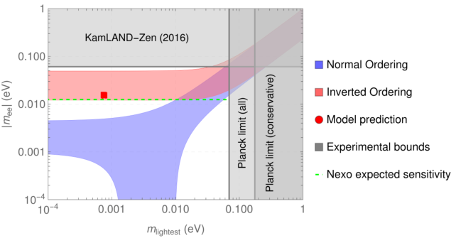
In our model the Majorana phases are approximately fixed as and , while the neutrino masses are also predicted to be around eV, eV, eV. Small deviations from these values are possible due to the experimental uncertainty on and the variance in . This automatically leads to a definite prediction of in our model:
| (29) |
Note that the term with in (28) interferes constructively to but is strongly suppressed by , while the term with interferes destructively. This is why the allowed points in the model are in the lower region of as seen in figure 4. The nEXO experiment is expected to test this model prediction in the future nEXO:2017nam; nEXO:2021ujk.
III.2 Normal ordering
In the Normal Ordering case, after imposing the correct charged lepton and neutrino masses at , a strong correlation appears between the mixing angles and in the neutrino sector. This correlation is not compatible with experimental constraints by more than , as can be seen in figure 5. Therefore, Normal Ordering of neutrino masses cannot be realised in this model.

IV Dark matter sector
The flavour symmetry has the additional property of stabilizing the lightest of the dark sector fields. In order to see how this mechanism works, we must first note that the singlets and the , triplets form a closed subset under the tensor products, i.e.
| (30) | |||||
| (31) |
We start by imposing the condition that all of the visible sector fields, i.e. the Standard Model fermions and Higgs, transform as either , or . This automatically implies that any effective operator formed by any arbitrary combination of SM particles, , will still transform under the same subgroup, i.e. as , or .
Consider now a field belonging to the dark sector and transforming as, for example, . It’s clear that the effective operator cannot be invariant under , because no operator of the type transforms as .
In conclusion, any symmetry invariant decay operator of a particle belonging to the dark sector must involve, at least, one dark sector particle in the final state and, thus, the lightest of them will necessarily be stable (see figure 6). In our model the dark matter could be either the lightest neutral mass eigenstate of the scalars , or the vector-like fermion , if lighter than the scalars.
Note that this is a generalised, non-Abelian version of the original scotogenic mechanism of Ma:2006km, where the stability of the dark matter candidate is enforced by a symmetry. This mechanism was extended to Abelian symmetries in Bonilla:2018ynb; CentellesChulia:2019gic. Moreover, in Lavoura:2012cv the authors present a similar mechanism for some discrete subgroups of .
While similar to the original scotogenic model, makes a clear distinction as already explained, even at the neutrino mass level: there are three independent scotogenic-like diagrams. Each set of unconnected fields and couplings were denoted with colours on Eqs. (7)-(9) for clarity. Regarding the dark matter, this means that the model contains a three-component DM, where the candidates are the lightest of each triad , and . Of course, after EWSB the neutral part of each scalar doublet will split into its CP-odd and CP-even components due to the usual term in equation (8). For more details on the scalar sector, we refer to Appendix B.
It is worth noting that while in most of the Scotogenic scenarios the scalar DM is normally preferred Avila:2021mwg, due to the problems of underproduction versus large cLFV for the fermion singlet candidate Vicente:2014wga, in this case the issue is largely mitigated. The fact that we have a three-component DM and no large contributions to cLFV, makes the singlet fermion DM case again phenomenologically interesting. Nevertheless, a complete study of the dark matter phenomenology is beyond the scope of this paper.
V Conclusions
We have presented a simple but extremely predictive variant of the scotogenic model. We promoted the scotogenic symmetry of the original work to a non-Abelian symmetry, which will satisfy the same role of stabilizing the dark matter candidates running in the neutrino mass loop. We considered that leptons, as well as the Higgs doublet , transform as triplets under the flavour symmetry, thus, resembling a 3HDM. These three scalar doublets are responsible for all the spontaneous symmetry breaking, which implies that the model does not need extra flavons in order to fit the experimental data. We found that such a model can, not only satisfy the current experimental constraints, but also lead to very strong and testable predictions in the close future. Fitting the charged lepton masses, and inside their allowed ranges, we automatically obtained the following predictions:
- •
Neutrino mass sum rule: .
- •
Only Inverted Ordering is realised.
- •
These two conditions together lead to eV, with some small deviations due to experimental uncertainty in .
- •
Strong correlation between and as shown in figure 2, testable in the near future Smith:2022ezh; NOvA:2016kwd.
- •
Majorana phases predicted to be around and , when all the other observables are in their experimental allowed ranges (see figure 3).
- •
The prediction of the Majorana phases and lead to , testable in future neutrinoless double beta decay experiments nEXO:2021ujk (see figure 4).
- •
The flavour symmetry ensures the stability of the dark matter candidate, which could be either fermionic or scalar. No other symmetries are required apart from the Standard Model gauge symmetries and the spontaneous symmetry breaking comes solely from the three Higgs gauge doublets arranged into a flavour triplet.
Appendix A Group
The group is a discrete, non-Abelian subgroup of Jurciukonis:2017mjp and belongs to the family of groups . It has four generators denoted by , , , and , which fulfill the relations,
| (32) |
| (33) |
All the elements of can be written in terms of the four generators as,
| (34) |
The representations of used for the fields multiplets in this model are , , , and . We choose the following basis for these representations: in the ,
| (35) |
where . In the representation,
| (36) |
Notice that the generators in the representation are the complex conjugate of the generators in the , and similarly between the , and .
It’s worth showing explicitly one of the key properties of that give rise to dark matter stability in the model presented, i.e. the singlet irreps together with and form a close subgroup. This can be seen by looking at the products (38)-(42).
| (37) |
with .
Expanding in components in the basis defined by (35) and (36), we have the tensor products,
| (38) |
| (39) |
| (40) |
| (41) |
| (42) |
The label , with , represent the nine different one dimensional irreps of , being the invariant singlet.
For further details of the properties of the group and the explicit expressions of the tensor products of dark sector fields we refer the reader to the second edition of the book “An Introduction to Non-Abelian Discrete Symmetries for Particle Physicists” Kobayashi:2022moq, since the first edition had inconsistencies in the representations used in the tensor products.
Appendix B Scalar sector
We now explicitly write down the relevant Lagrangian terms that lead to the masses of the scalars and . These are given by equations (8) and
| (43) | |||||
where the sub-index outside a bracket represent the different contractions under to the trivial singlet. Explicitly,
| (44) | |||||
| (45) | |||||
| (46) | |||||
| (47) | |||||
| (48) | |||||
| (49) | |||||
| (50) |
with .
As usual, the scalars and can be written down into their components as,
| (51) | |||||
| (52) |
After EWSB, the charged components of each and remain as mass eigenstates, with masses
| (53) | |||||
| (54) |
in the limit (see (3)).
On the other hand, the neutral components mix through the terms given in equation (8). Assuming a CP conserving scalar potential, which implies , the mixing only happens among CP-odd and CP-even scalars and in pairs , and . Respectively, the mass matrices for each pair is given by
| (55) | |||
| (56) | |||
| (57) |
By choosing appropriate signs for the couplings one can make sure that a neutral component is the lightest field of each set.
Appendix C Acknowledgements
The authors want to thank Andreas Trautner for double covering us with wisdom and Rahul Srivastava for helpful comments. We also thank professor Luís Lavoura and professor Martin K. Hirsch for helpful insight. O.M. is supported by the Spanish grant PID2020-113775GB-I00 (AEI/10.13039/501100011033) and Programa Santiago Grisolía (No. GRISOLIA/2020/025). R.C. is supported by the Alexander von Humboldt Foundation Fellowship.
References
- (1) P. Minkowski, “ at a Rate of One Out of Muon Decays?,” Phys. Lett. B 67 (1977) 421–428.
- (2) T. Yanagida, “Horizontal gauge symmetry and masses of neutrinos,” Conf. Proc. C 7902131 (1979) 95–99.
- (3) M. Gell-Mann, P. Ramond, and R. Slansky, “Complex Spinors and Unified Theories,” vol. C790927, pp. 315–321. 1979. arXiv:1306.4669 [hep-th].
- (4) R. N. Mohapatra and G. Senjanović, “Neutrino mass and spontaneous parity nonconservation,” Phys. Rev. Lett. 44 (Apr, 1980) 912–915. https://link.aps.org/doi/10.1103/PhysRevLett.44.912.
- (5) J. Schechter and J. W. F. Valle, “Neutrino Masses in SU(2) x U(1) Theories,” Phys. Rev. D 22 (1980) 2227.
- (6) J. Schechter and J. W. F. Valle, “Neutrino decay and spontaneous violation of lepton number,” Phys. Rev. D25 774.
- (7) E. Ma, “Pathways to naturally small neutrino masses,” Phys.Rev.Lett. 81 (1998) 1171–1174.
- (8) S. Centelles Chuliá, R. Srivastava, and J. W. F. Valle, “Seesaw roadmap to neutrino mass and dark matter,” Phys. Lett. B 781 (2018) 122–128, arXiv:1802.05722 [hep-ph].
- (9) S. Centelles Chuliá, R. Srivastava, and A. Vicente, “The inverse seesaw family: Dirac and Majorana,” JHEP 03 (2021) 248, arXiv:2011.06609 [hep-ph].
- (10) Planck Collaboration, N. Aghanim et al., “Planck 2018 results. VI. Cosmological parameters,” arXiv:1807.06209 [astro-ph.CO].
- (11) F. Bonnet, M. Hirsch, T. Ota, and W. Winter, “Systematic study of the d=5 Weinberg operator at one-loop order,” JHEP 1207 (2012) 153, arXiv:1204.5862 [hep-ph].
- (12) Y. Farzan, S. Pascoli, and M. A. Schmidt, “Recipes and Ingredients for Neutrino Mass at Loop Level,” JHEP 03 (2013) 107, arXiv:1208.2732 [hep-ph].
- (13) D. Aristizabal Sierra, A. Degee, L. Dorame, and M. Hirsch, “Systematic classification of two-loop realizations of the Weinberg operator,” JHEP 1503 (2015) 040, arXiv:1411.7038 [hep-ph].
- (14) R. Cepedello, M. Hirsch, and J. Helo, “Loop neutrino masses from operator,” JHEP 1707 (2017) 079, arXiv:1705.01489 [hep-ph].
- (15) C.-Y. Yao and G.-J. Ding, “Systematic Study of One-Loop Dirac Neutrino Masses and Viable Dark Matter Candidates,” Phys.Rev. D96 (2017) 095004, arXiv:1707.09786 [hep-ph].
- (16) R. Cepedello, R. M. Fonseca, and M. Hirsch, “Systematic classification of three-loop realizations of the Weinberg operator,” JHEP 1810 (2018) 197, arXiv:1807.00629 [hep-ph].
- (17) C. Klein, M. Lindner, and S. Ohmer, “Minimal Radiative Neutrino Masses,” JHEP 1903 (2019) 018, arXiv:1901.03225 [hep-ph].
- (18) S. Centelles Chuliá, R. Cepedello, E. Peinado, and R. Srivastava, “Systematic classification of two loop = 4 Dirac neutrino mass models and the Diracness-dark matter stability connection,” JHEP 10 (2019) 093, arXiv:1907.08630 [hep-ph].
- (19) Y. Cai, J. Herrero-García, M. A. Schmidt, A. Vicente, and R. R. Volkas, “From the trees to the forest: a review of radiative neutrino mass models,” Front.in Phys. 5 (2017) 63, arXiv:1706.08524 [hep-ph].
- (20) C. Bonilla, S. Centelles-Chuliá, R. Cepedello, E. Peinado, and R. Srivastava, “Dark matter stability and Dirac neutrinos using only Standard Model symmetries,” Phys. Rev. D 101 no. 3, (2020) 033011, arXiv:1812.01599 [hep-ph].
- (21) S. Centelles Chuliá, R. Cepedello, E. Peinado, and R. Srivastava, “Scotogenic dark symmetry as a residual subgroup of Standard Model symmetries,” Chin. Phys. C 44 no. 8, (2020) 083110, arXiv:1901.06402 [hep-ph].
- (22) R. Srivastava, C. Bonilla, and E. Peinado, “The role of residual symmetries in dark matter stability and the neutrino nature,” LHEP 2 no. 1, (2019) 124, arXiv:1903.01477 [hep-ph].
- (23) E. Ma, “Verifiable radiative seesaw mechanism of neutrino mass and dark matter,” Phys. Rev. D 73 (2006) 077301, arXiv:hep-ph/0601225.
- (24) N. Rojas, R. Srivastava, and J. W. F. Valle, “Simplest Scoto-Seesaw Mechanism,” Phys. Lett. B 789 (2019) 132–136, arXiv:1807.11447 [hep-ph].
- (25) S. K. Kang, O. Popov, R. Srivastava, J. W. Valle, and C. A. Vaquera-Araujo, “Scotogenic dark matter stability from gauged matter parity,” arXiv:1902.05966 [hep-ph].
- (26) J. Leite, O. Popov, R. Srivastava, and J. W. F. Valle, “A theory for scotogenic dark matter stabilised by residual gauge symmetry,” Phys. Lett. B 802 (2020) 135254, arXiv:1909.06386 [hep-ph].
- (27) D. M. Barreiros, F. R. Joaquim, R. Srivastava, and J. W. F. Valle, “Minimal scoto-seesaw mechanism with spontaneous CP violation,” JHEP 04 (2021) 249, arXiv:2012.05189 [hep-ph].
- (28) D. Borah, M. Dutta, S. Mahapatra, and N. Sahu, “Singlet-Doublet Self-interacting Dark Matter and Radiative Neutrino Mass,” arXiv:2112.06847 [hep-ph].
- (29) P. Escribano and A. Vicente, “An ultraviolet completion for the Scotogenic model,” Phys. Lett. B 823 (2021) 136717, arXiv:2107.10265 [hep-ph].
- (30) S. Mandal, R. Srivastava, and J. W. F. Valle, “The simplest scoto-seesaw model: WIMP dark matter phenomenology and Higgs vacuum stability,” Phys. Lett. B 819 (2021) 136458, arXiv:2104.13401 [hep-ph].
- (31) L. Sarma, B. B. Boruah, and M. K. Das, “Neutrinoless Double Beta Decay in a Flavor Symmetric Scotogenic Model,” Springer Proc. Phys. 265 (2022) 217–222.
- (32) E. Ma, “Scotogenic Dirac Neutrinos with Freeze-In Dark Matter,” arXiv:2202.13031 [hep-ph].
- (33) M. Sarazin, J. Bernigaud, and B. Herrmann, “Dark matter and lepton flavour phenomenology in a singlet-doublet scotogenic model,” JHEP 12 (2021) 116, arXiv:2107.04613 [hep-ph].
- (34) T. Kajita, “Nobel Lecture: Discovery of atmospheric neutrino oscillations,” Rev.Mod.Phys. 88 (2016) 030501.
- (35) A. B. McDonald, “Nobel Lecture: The Sudbury Neutrino Observatory: Observation of flavor change for solar neutrinos,” Rev.Mod.Phys. 88 (2016) 030502.
- (36) Particle Data Group Collaboration, P. A. Zyla et al., “Review of Particle Physics,” PTEP 2020 no. 8, (2020) 083C01.
- (37) S. F. King, “Models of Neutrino Mass, Mixing and CP Violation,” J. Phys. G 42 (2015) 123001, arXiv:1510.02091 [hep-ph].
- (38) F. Feruglio and A. Romanino, “Lepton flavor symmetries,” Rev. Mod. Phys. 93 no. 1, (2021) 015007, arXiv:1912.06028 [hep-ph].
- (39) M. Hirsch, S. Morisi, E. Peinado, and J. W. F. Valle, “Discrete dark matter,” Phys. Rev. D 82 (2010) 116003, arXiv:1007.0871 [hep-ph].
- (40) L. Lavoura, S. Morisi, and J. W. F. Valle, “Accidental Stability of Dark Matter,” JHEP 02 (2013) 118, arXiv:1205.3442 [hep-ph].
- (41) M. S. Boucenna, S. Morisi, E. Peinado, Y. Shimizu, and J. W. F. Valle, “Predictive discrete dark matter model and neutrino oscillations,” Phys. Rev. D 86 (2012) 073008, arXiv:1204.4733 [hep-ph].
- (42) E. Ma, “Scotogenic cobimaximal Dirac neutrino mixing from and ,” Eur. Phys. J. C 79 no. 11, (2019) 903, arXiv:1905.01535 [hep-ph].
- (43) F. J. de Anda, O. Medina, J. W. F. Valle, and C. A. Vaquera-Araujo, “Scotogenic Majorana neutrino masses in a predictive orbifold theory of flavor,” Phys. Rev. D 105 no. 5, (2022) 055030, arXiv:2110.06810 [hep-ph].
- (44) Y. BenTov and A. Zee, “Lepton Private Higgs and the discrete group \Sigma(81),” Nucl. Phys. B 871 (2013) 452–484, arXiv:1202.4234 [hep-ph].
- (45) C. Hagedorn, M. A. Schmidt, and A. Y. Smirnov, “Lepton Mixing and Cancellation of the Dirac Mass Hierarchy in SO(10) GUTs with Flavor Symmetries T(7) and Sigma(81),” Phys. Rev. D 79 (2009) 036002, arXiv:0811.2955 [hep-ph].
- (46) K. Abe, H. Aihara, C. Andreopoulos, I. Anghel, A. Ariga, T. Ariga, R. Asfandiyarov, M. Askins, J. Back, P. Ballett, et al., “A long baseline neutrino oscillation experiment using j-parc neutrino beam and hyper-kamiokande,” arXiv preprint arXiv:1412.4673 (2014) .
- (47) Hyper-Kamiokande Collaboration, K. Abe et al., “Physics potentials with the second Hyper-Kamiokande detector in Korea,” PTEP 2018 no. 6, (2018) 063C01, arXiv:1611.06118 [hep-ex].
- (48) DUNE Collaboration, B. Abi et al., “Long-baseline neutrino oscillation physics potential of the DUNE experiment,” Eur. Phys. J. C 80 no. 10, (2020) 978, arXiv:2006.16043 [hep-ex].
- (49) JUNO Collaboration, F. An et al., “Neutrino Physics with JUNO,” J. Phys. G 43 no. 3, (2016) 030401, arXiv:1507.05613 [physics.ins-det].
- (50) J. Cao et al., “Muon-decay medium-baseline neutrino beam facility,” Phys. Rev. ST Accel. Beams 17 (2014) 090101, arXiv:1401.8125 [physics.acc-ph].
- (51) KamLAND-Zen Collaboration, A. Gando et al., “Search for Majorana Neutrinos near the Inverted Mass Hierarchy Region with KamLAND-Zen,” Phys. Rev. Lett. 117 no. 8, (2016) 082503, arXiv:1605.02889 [hep-ex]. [Addendum: Phys.Rev.Lett. 117, 109903 (2016)].
- (52) GERDA Collaboration, M. Agostini et al., “GERDA results and the future perspectives for the neutrinoless double beta decay search using 76Ge,” Int.J.Mod.Phys. A33 (2018) 1843004.
- (53) M. Agostini et al., “Background-free search for neutrinoless double- decay of 76Ge with GERDA,” arXiv:1703.00570 [nucl-ex].
- (54) CUORE Collaboration, C. Alduino et al., “First Results from CUORE: A Search for Lepton Number Violation via Decay of 130Te,” Phys.Rev.Lett. 120 (2018) 132501, arXiv:1710.07988 [nucl-ex].
- (55) NEMO-3 Collaboration, R. Arnold et al., “Measurement of the 2 decay half-life of 150Nd and a search for 0 decay processes with the full exposure from the NEMO-3 detector,” Phys.Rev. D94 (2016) 072003, arXiv:1606.08494 [hep-ex].
- (56) EXO-200 Collaboration, J. Albert et al., “Search for Majorana neutrinos with the first two years of EXO-200 data,” Nature 510 (2014) 229–234, arXiv:1402.6956 [nucl-ex].
- (57) H. Georgi and D. V. Nanopoulos, “Suppression of Flavor Changing Effects From Neutral Spinless Meson Exchange in Gauge Theories,” Phys. Lett. B 82 (1979) 95–96.
- (58) I. de Medeiros Varzielas, I. P. Ivanov, and M. Levy, “Exploring multi-Higgs models with softly broken large discrete symmetry groups,” Eur. Phys. J. C 81 no. 10, (2021) 918, arXiv:2107.08227 [hep-ph].
- (59) I. P. Ivanov and E. Vdovin, “Discrete symmetries in the three-Higgs-doublet model,” Phys. Rev. D 86 (2012) 095030, arXiv:1206.7108 [hep-ph].
- (60) V. Keus, S. F. King, and S. Moretti, “Three-Higgs-doublet models: symmetries, potentials and Higgs boson masses,” JHEP 01 (2014) 052, arXiv:1310.8253 [hep-ph].
- (61) I. P. Ivanov and C. C. Nishi, “Symmetry breaking patterns in 3HDM,” JHEP 01 (2015) 021, arXiv:1410.6139 [hep-ph].
- (62) M. Maniatis and O. Nachtmann, “Stability and symmetry breaking in the general three-Higgs-doublet model,” JHEP 02 (2015) 058, arXiv:1408.6833 [hep-ph]. [Erratum: JHEP 10, 149 (2015)].
- (63) J. Vergeest, M. Zrałek, B. Dziewit, and P. Chaber, “Lepton masses and mixing in a three-Higgs doublet model,” arXiv:2203.03514 [hep-ph].
- (64) A. E. C. Hernández, S. Kovalenko, M. Maniatis, and I. Schmidt, “Fermion mass hierarchy and g 2 anomalies in an extended 3HDM Model,” JHEP 10 (2021) 036, arXiv:2104.07047 [hep-ph].
- (65) I. de Medeiros Varzielas and D. Ivo, “Softly-broken or 3HDMs with stable states,” Eur. Phys. J. C 82 no. 5, (2022) 415, arXiv:2202.00681 [hep-ph].
- (66) T. Kobayashi, H. Ohki, H. Okada, Y. Shimizu, and M. Tanimoto, An Introduction to Non-Abelian Discrete Symmetries for Particle Physicists. 1, 2022.
- (67) G. Passarino and M. J. G. Veltman, “One loop corrections for annihilation into in the Weinberg model,” Nucl. Phys. B160 (1979) 151–207.
- (68) P. Escribano, M. Reig, and A. Vicente, “Generalizing the Scotogenic model,” JHEP 07 (2020) 097, arXiv:2004.05172 [hep-ph].
- (69) W. Rodejohann and J. W. F. Valle, “Symmetrical Parametrizations of the Lepton Mixing Matrix,” Phys. Rev. D 84 (2011) 073011, arXiv:1108.3484 [hep-ph].
- (70) IceCube Collaboration, M. G. Aartsen et al., “Measurement of Atmospheric Tau Neutrino Appearance with IceCube DeepCore,” Phys. Rev. D 99 no. 3, (2019) 032007, arXiv:1901.05366 [hep-ex].
- (71) Super-Kamiokande Collaboration, K. Abe et al., “Atmospheric neutrino oscillation analysis with external constraints in Super-Kamiokande I-IV,” Phys. Rev. D 97 no. 7, (2018) 072001, arXiv:1710.09126 [hep-ex].
- (72) T2K Collaboration, K. Abe et al., “Improved constraints on neutrino mixing from the T2K experiment with protons on target,” Phys. Rev. D 103 no. 11, (2021) 112008, arXiv:2101.03779 [hep-ex].
- (73) A. Himmel, “New oscillation results from the nova experiment,” July, 2020. https://doi.org/10.5281/zenodo.3959581.
- (74) Daya Bay Collaboration, D. Adey et al., “Measurement of the Electron Antineutrino Oscillation with 1958 Days of Operation at Daya Bay,” Phys. Rev. Lett. 121 no. 24, (2018) 241805, arXiv:1809.02261 [hep-ex].
- (75) KamLAND Collaboration, A. Gando et al., “Constraints on from A Three-Flavor Oscillation Analysis of Reactor Antineutrinos at KamLAND,” Phys. Rev. D 83 (2011) 052002, arXiv:1009.4771 [hep-ex].
- (76) Planck Collaboration, N. Aghanim et al., “Planck 2018 results. VI. Cosmological parameters,” Astron. Astrophys. 641 (2020) A6, arXiv:1807.06209 [astro-ph.CO]. [Erratum: Astron.Astrophys. 652, C4 (2021)].
- (77) KATRIN Collaboration, M. Aker et al., “Direct neutrino-mass measurement with sub-electronvolt sensitivity,” Nature Phys. 18 no. 2, (2022) 160–166, arXiv:2105.08533 [hep-ex].
- (78) KATRIN Collaboration, M. Aker et al., “KATRIN: Status and Prospects for the Neutrino Mass and Beyond,” arXiv:2203.08059 [nucl-ex].
- (79) K. Kyutoku and K. Kashiyama, “Detectability of thermal neutrinos from binary-neutron-star mergers and implication to neutrino physics,” Phys. Rev. D 97 no. 10, (2018) 103001, arXiv:1710.05922 [astro-ph.HE].
- (80) P. F. de Salas, D. V. Forero, S. Gariazzo, P. Martínez-Miravé, O. Mena, C. A. Ternes, M. Tórtola, and J. W. F. Valle, “2020 global reassessment of the neutrino oscillation picture,” JHEP 02 (2021) 071, arXiv:2006.11237 [hep-ph].
- (81) I. Esteban, M. C. Gonzalez-Garcia, M. Maltoni, T. Schwetz, and A. Zhou, “The fate of hints: updated global analysis of three-flavor neutrino oscillations,” JHEP 09 (2020) 178, arXiv:2007.14792 [hep-ph].
- (82) A. Marrone, E. Lisi, A. Palazzo, D. Montanino, and F. Capozzi, “Global fits to neutrino oscillations: status and prospects,” PoS EPS-HEP2015 (2015) 093.
- (83) P. Chen, S. Centelles Chuliá, G.-J. Ding, R. Srivastava, and J. W. F. Valle, “Neutrino Predictions from Generalized CP Symmetries of Charged Leptons,” JHEP 07 (2018) 077, arXiv:1802.04275 [hep-ph].
- (84) P. Chen, S. Centelles Chuliá, G.-J. Ding, R. Srivastava, and J. W. F. Valle, “CP symmetries as guiding posts: Revamping tribimaximal mixing. II.,” Phys. Rev. D 100 no. 5, (2019) 053001, arXiv:1905.11997 [hep-ph].
- (85) nEXO Collaboration, J. B. Albert et al., “Sensitivity and Discovery Potential of nEXO to Neutrinoless Double Beta Decay,” Phys. Rev. C 97 no. 6, (2018) 065503, arXiv:1710.05075 [nucl-ex].
- (86) nEXO Collaboration, G. Adhikari et al., “nEXO: neutrinoless double beta decay search beyond 1028 year half-life sensitivity,” J. Phys. G 49 no. 1, (2022) 015104, arXiv:2106.16243 [nucl-ex].
- (87) I. M. Ávila, G. Cottin, and M. A. Díaz, “Revisiting the scotogenic model with scalar dark matter,” J. Phys. G 49 no. 6, (2022) 065001, arXiv:2108.05103 [hep-ph].
- (88) A. Vicente and C. E. Yaguna, “Probing the scotogenic model with lepton flavor violating processes,” JHEP 02 (2015) 144, arXiv:1412.2545 [hep-ph].
- (89) NOvA Collaboration, E. Smith, “Neutrino Oscillation Results from the NOvA Experiment,” PoS PANIC2021 (2022) 289.
- (90) NOvA Collaboration, P. Adamson et al., “First measurement of electron neutrino appearance in NOvA,” Phys. Rev. Lett. 116 no. 15, (2016) 151806, arXiv:1601.05022 [hep-ex].
- (91) D. Jurciukonis and L. Lavoura, “GAP listing of the finite subgroups of U (3) of order smaller than 2000,” PTEP 2017 no. 5, (2017) 053A03, arXiv:1702.00005 [math.RT].