Generating Topological Structure of Floorplans from Room Attributes
Abstract
Analysis of indoor spaces requires topological information. In this paper, we propose to extract topological information from room attributes using what we call Iterative and adaptive graph Topology Learning (ITL). ITL progressively predicts multiple relations between rooms; at each iteration, it improves node embeddings, which in turn facilitates generation of a better topological graph structure. This notion of iterative improvement of node embeddings and topological graph structure is in the same spirit as chen2020iterative. However, while chen2020iterative computes the adjacency matrix based on node similarity, we learn the graph metric using a relational decoder to extract room correlations. Experiments using a new challenging indoor dataset validate our proposed method. Qualitative and quantitative evaluation for layout topology prediction and floorplan generation applications also demonstrate the effectiveness of ITL.
1 Introduction
Indoor home modeling enables practical applications such as virtual home tours, indoor navigation, and house design. Augmenting raw models with topological information enhances their value by providing semantic-level knowledge of room identity and arrangement. This, in turn, facilitates indoor understanding (e.g., style classification) and more home-related applications such as remote home shopping (through similarity-based search) and pricing.

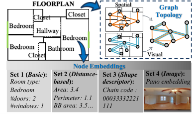
Motivated by the lack of large-scale floorplan topology information in real estate listing websites (e.g. Airbnb, Zillow, Apartments), we propose to extract it using available, or derivable, room-level signals encoded into a graph convolutional network (GCN). Topological information of a floorplan can be easily embedded in a graph, where nodes represent rooms and edges encode relations between them. Room adjacency (Fig. 1) is characterized as having a spatial connection; the spatial connection can be either visual (if there is a door or opening between rooms) or non-visual (if there is no door or opening). In other words, spatial connectivity provides the information about ”which room is adjacent to which room”, while visual connectivity provides information about ”which room connects which room”. To handle the multiple relationships and predict both connection types, we propose the multi-relational GAT as an extension to GAT velivckovic2017graph. Here, we treat each relation as a sub-graph and then fuse the information with a weighted summation of both.
We propose an iterative and adaptive learning mechanism to progressively predict multiple relationships between rooms with given or precomputed attributes in an indoor environment. Note that conventional similarity metric learning approaches (e.g. chen2020iterative) cannot simply be applied to our application due to high levels of similarity between our nodes (e.g., two similar non-adjacent bedrooms). Also, current similarity metric learning approaches can be extended to multi-relational graphs only when the graph-structure is available. Thus, we progressively learn the graph metric using a relational decoder to make better use of the containment relationship between the spatial and visual edges (i.e., visual edges should be a subset of spatial edges).
Our contributions are:
- •
First data-driven method (to our knowledge) to automatically generate floorplan topology using room attributes. Multi-relational (MR) GAT and MR decoder are proposed to model the containment relationship between edges.
- •
We propose a new iterative learning mechanism to predict multiple relations between graph nodes from scratch, in the absence of any initial topology structure.
- •
We demonstrate the effectiveness of the proposed method for indoor applications (i.e. realistic floorplan generation) by employing HouseGAN nauata2020house on the outputs of our method.
2 Related Work
2.1 Topological relationships of 2D/3D floorplans
The topological relationships inherent to 2D floorplans have been widely studied in different fields from different perspectives goodman2019machine. To assist in the task of navigation, Portugal and Rocha portugal2012extracting derived a topological graph-based representation from a grid map of floorplan. Lin et al. lin2017hybrid merged a topology graph and a grid model to boost the efficiency of spatial analysis and to provide positional information. Nauata et al. nauata2020house showed that the spatial connectivity of room boosts the performance of floorplan generation task. In hu2020graph2plan, room connectivity provided by users are used as constraints to generate floorplans. More recently, armeni20193d proposed a layered-graph representation, 3D Scene Graph, to facilitate the holistic understanding of indoor spaces.
A popular approach to extract topological relationships is detecting high-level information from grid maps thrun1996integrating; joo2010generating; portugal2012extracting; yang2015generation; sithole2018indoor. The main problem is that grid maps are often unavailable or difficult to obtain in some applications. We argue that it is too restrictive to ask the user or designer to provide such detailed information including both room attributes and connections. This huge drawback can be addressed by extracting topological relationships from room attributes, which is largely unexplored in the literature. By contrast, we propose to leverage the underlying relational information between rooms to learn topological information from room attributes. The learned topological information can then facilitate indoor understanding (e.g. LayoutGMN patil2021layoutgmn) and more home-related applications such as floorplan generation (e.g. HouseGAN nauata2020house, HouseGAN++ nauata2021house).
2.2 Graph neural networks
GNNs model graph dependencies via message passing between nodes, and have been thoroughly studied skarding2020foundations; wu2020comprehensive; zhou2018graph. Recently, GNNs have gained increasing attention in various domains, including knowledge graphs schlichtkrull2018modeling; shang2019end; zhu2020collective, recommendation systems ying2018graph; zhang2020gcn, and other computer vision tasks xu2017scene; xue2020learning. Multi-relational (MR) GNNs are more intuitive for indoor related tasks, as floorplans typically encode multi-relational connectivity between rooms. To handle multi-relational graphs, R-GCN schlichtkrull2018modeling extends GCN with relation-specific linear transformation. W-GCN shang2019end utilizes relation-specific learnable weights during information aggregation. COMP-GCN vashishth2019composition gains extra information by jointly embedding both nodes and relations in a relational graph.
The aforementioned methods are mainly designed for knowledge graph with clean graph structure. However, learning floorplan topology is fundamentally different from these tasks as the graph structure is completely unknown or severely missing. Most of the aforementioned works fail to pass messages along the model when structural information is missing. To directly adopt these MR-GNNs on floorplan topology learning task, we first need to add initial structures (e.g. fully connected graphs, kNN graphs), which will introduce noise to the graph and lead to inaccurate predictions. Rather than using regular MR-GNNs directly, we extend GAT to multi-relational (MR) GAT for message passing and adopt a MR-decoder to utilize the containment relationship among edge types and learn more precise room connections.
2.3 Iterative graph learning
Most GNN methods velivckovic2017graph; chami2019hyperbolic; kipf2016semi are only applicable when the graph structure is available and clean. To address this limitation, researchers have explored methods xue2020learning; franceschi2019learning; grover2019graphite to automatically generate and iteratively update the graph with (previously) unknown structure. More recently, chen2020iterative cast the graph learning problem as similarity metric learning and proposed to iteratively learn the graph structure and embeddings. Though promising performance was shown on knowledge graphs, it is less effective on floorplan graphs, where connections are not determined only by similarity of two nodes. For example, bedrooms in a house usually have similar embeddings; however, they are rarely visually connected, and their spatial connectivity is not guaranteed.
3 Problem Definition
In this paper, our goal is to predict a set of topological relations between the nodes of a graph representing an indoor environment. More specifically, we start with a set of given node attributes (room attributes in our case) and the goal is to predict spatial and/or visual connectivity between the given nodes. Our final learned graph embeddings can be used to infer topological structure of indoor environments from scratch, i.e. no links provided, or to complete the topology of partial layouts. In this section, we first introduce the dataset we are using, then go over three problem definition including graph structure generation, graph structure completion, and the application of floorplan generation.
3.1 Floorplan dataset
The Zillow Indoor Dataset (ZInD)11 1 https://github.com/zillow/zind cruz2021zillow provides 360∘ panoramas, room layouts, and floorplans collected from 1,575 real unfurnished homes. In total, it contains 2737 floorplans, from which we retrieved 1,217 and constructed graphs containing nodes and multi-relational edges. The data statistics are summarized in Table 1. More details (e.g. node and edge distributions) of the dataset are provided in the supplementary material.
We then represent each floorplan as a graph. Each node in a floorplan represents a room, and edges represent the connectivity between two rooms. We define two types of edges, spatial and visual (Fig. 12). Spatial edges are defined by room-room adjacency in a floorplan, while visual connections represent a sub-set of the spatial edges when two rooms share a door or an opening. We represent nodes using four types of room features:
- •
Basic room information (Set 1): room type, number of doors, windows, and openings of the room.
- •
Distance-based features (Set 2): perimeter and area of the room, maximum length and width of walls, and ratio between room area and its bounding box area.
- •
Shape descriptors (Set 3): we use the chain code freeman1961encoding to represent the shape of a room. The chain code is extracted by traversing the boundary of the object and recording the direction of each step.
- •
Image features (Set 4): extracted from panoramas using embeddings from a scene classification model cruz2021zillow.
Note that all room attributes are invariant to translation and rotation. Features in Sets 1 and 4 are also invariant to scale, while the other two are not. Fig. 2 shows an example of a floorplan, input attributes and constructed graphs from the dataset. Detailed description of topology and attribute extraction are in the supplementary material. In our work, we assume all these room-level attributes are given. This is the input to our system, and our goal is to predict the layout. In practice, these room attributes can be derived from the panorama images, either manually (e.g. cruz2021zillow; armeni2017joint) or automatically from SOTA algorithms for scene classification (e.g. liu2019indoor; ismail2018understanding) and room layout estimation (e.g. cabral2014piecewise; pintore2019automatic; yang2019dula). In Table 5 we study the effect of the different attributes.
| Total | Avg | (Min, Max) | |
|---|---|---|---|
| # of graphs | 1217 | – | – |
| # of nodes | 12253 | 10.07 | (2, 30) |
| # of spatial edges | 55242 | 45.39 | (8, 144) |
| # of visual edges | 12138 | 9.97 | (2, 32) |
3.2 Graph structure generation
The goal of graph structure generation is to predict different types of connections (i.e. visual, wall, and spatial connections) given only room attributes and without any structure information. The adjacency matrix of the input graph is an identity matrix, meaning that each room is connected to itself and not to any other rooms in the floorplan. The dataset is split across graphs. We use 700 floorplan graphs for training, 200 floorplans for validation, and the rest (i.e., 317 floorplans) for testing. All edges in training graphs are in the training set, and the model is asked to predict unseen links (i.e. all edges) for test graphs.
3.3 Graph structure completion
Given room attributes and partial spatial structure information, the goal is to complete the spatial connection (i.e. the rooms are connected or not) and predict the specific type of the connection (i.e. the rooms are connected by door (visual) or wall). Let be the adjacency matrix of the graph generated from original spatial edges of a floor plan; we randomly remove a subset of spatial edges (e.g. 20% - 80% of edges) and use the remaining observations to generate an incomplete adjacency matrix . We use the same data split as graph structure generation task (i.e. 700 graphs for training, 200 for validation and 316 for testing). All edges in training graphs are used for training. We then evaluate on a fixed set of 20% of connections that was not observed.

3.4 Indoor application using generated topology
The proposed learned representation includes rich information about an indoor environment. We show how this topological information can benefit the challenging task of home layout generation, from room-level attributes. As demonstration, we use HouseGAN nauata2020house, which takes in room attributes and room spatial information. We replace the ground truth (GT) room connections with our estimated graph topology, and show that it can generate compatible results with using the GT. Following nauata2020house, results are evaluated in terms of realism, diversity, and compatibility. Qualitative result shows the realism of generate floorplan. Diversity and compatibility are measured by the Frechet Inception Distance (FID) scores and graph edit distance sanfeliu1983distance (GED), respectively. We show a significant performance boost on HouseGAN nauata2020house by adopting the topological information generated from the proposed method. Note that we do not train end-to-end, as HouseGAN only includes a single edge type (i.e. spatial edges), whereas our model predicts both spatial and visual connectivity. For floorplan generation task, we fine-tune the pre-trained HouseGAN model with our dataset and follow the same setting as in HouseGAN. Since the room types in HouseGAN are different from ours, we map our room types to match theirs.
4 Methodology
The goal of this paper is to use relational information between graph nodes to predict its topology, when very little to no topological information is available. By comparison, traditional approaches assume a percentage of edges are available and aim to predict the rest. The architecture of our proposed model is shown in Fig. 3. Our architecture allows us to jointly predict both visual and spatial edges. We first generate an incomplete graph with an identity adjacency matrix from a floor plan. The incomplete graph is then fed into an iterative encoder, which recursively updates graph topology and node embeddings. With node embeddings as the input, the multi-relational (MR) decoder then learns more precise room connections by leveraging the containment relationship between spatial and visual edges (i.e. visual edges should be a subset of spatial edges).
Let be an undirected graph, where is a set of nodes with node attributes . is the feature dimension of each node. The true adjacency matrix is formulated from edges , where is the number of relation types in the graph. Suppose the initial adjacency matrix has missing or incomplete information. The objective of the model is to complete the graph topology by exploiting potential relationships based on room attributes. Specifically, an iterative encoding function is applied to transform the initial features to a new feature representation. The multi-relational decoding function, which takes the new feature representations as input, is then used to predict the probability of whether or not an edge exists between pairs of nodes , as well as the edge type.
We predict multiple types of edges (i.e. spatial and visual edges). Since visual edges are a subset of spatial edges, we split spatial edges into two exclusive sets: door (i.e. visual) connectivity and wall connectivity. We then jointly predict all three types of edges to fully explore and utilize the containment relationship among them.
4.1 Iterative encoder
The iterative encoder recursively augments the initial graph topology and node embeddings to improve the performance of downstream prediction tasks. The initial node embeddings and adjacency matrix are the input of our iterative encoder. is the original node (room) attributes, and is set to either an identity matrix or an incomplete adjacency matrix. In each iteration , we first update the graph topology from to using a multi-relational scoring function, then compute new node embeddings based on and . Inspired by shang2019end, we extend GAT velivckovic2017graph to multi-relation GAT (MR-GAT) for message passing, where we treat each relation as a subgraph and then conduct weighted summation on all the subgraphs. The process of each iteration block can be expressed as:
| (1) | ||||
where and denote the function to update graph topology and node embeddings, respectively.
4.1.1 Updating graph topology
Previous approaches (e.g. chen2020iterative; kipf2016variational) that model the graph structure learning problem as similarity metric learning have shown promising performance on knowledge graphs. However, these methods are unable to cope with the floorplan graphs, in which connections are not determined only by the similarity of two nodes. Moreover, similarity metric learning can only generate a single matrix to represent one type of room relationship given the node embeddings, and hence cannot be applied to multi-relational graphs. Instead, we use a multi-relational scoring function to make better use of the containment relationship between spatial and visual edges. Specifically, we decompose spatial connectivity into door (visual) and wall connectivity and predict them separately. Then spatial edges can be calculated by summing up door and wall edges. The prediction of door and wall edges can further be restricted by the binary cross-entropy loss applied on spatial edges. Therefore, the probability that node and are connected by relation (i.e. door, wall, or spatial) at the -th iteration is updated by:
| (2) |
where and are the embeddings of node and . The scoring function is implemented with three fully-connected layers.
4.1.2 Updating node embeddings
MR-GAT is employed to handle multi-relation message passing, which measures the various types of relationships differently during aggregation and learns the weights adaptively during network training. Specifically, the encoder treats a multi-relation floorplan graph as multiple single-relation subgraphs, where each subgraph represents a specific type of connection (i.e. door or wall connection). For each subgraph with relation , we then conduct self-attention on the nodes to indicate the importance of node ’s features to node . We first apply an attention mechanism , which is the same as velivckovic2017graph, on the concatenated features of node and to compute the attention coefficient, then use the softmax function to normalize it across all choices of in each relation . The attention coefficients can be expressed as:
| (3) | ||||
where [, ] represents concatenation operation, and denotes sets of rooms that are connected with node by relation (i.e. wall or door connection). Hence the output of each subgraph can be expressed as:
| (4) |
where is the weight matrix of linear transformation for relation .
Then we extend GAT to MR-GAT by performing weight summation on subgraphs of different relations . The MR-GAT determines how much weights to give to each subgraph when fusing the GAT embeddings for a node. Hence, the embeddings of node can be updated by:
| (5) |
where denotes the attention coefficient for each subgraph , and is learnt during training. As shown in Fig. 4, this process is essentially matrix multiplication. For each subgraph , we first conduct self-attention on the nodes. Then the attention-weighted adjacency matrix will be the weighted sum of the output subgraphs, and can be written as:
| (6) |
In matrix form, the node embedding update can be expressed as:
| (7) |
4.2 Link prediction decoder
Similarly, we take advantage of the containment relationship between spatial and visual edges and apply the same MR decoder for the link prediction task by decomposing spatial connectivity into door and wall connectivity, and then predicting them separately. After the iterative encoder, the model splits into two decoder branches, which predict door and wall edges separately. The two decoders have the same structure, each containing three fully-connected layers. Then, the door and wall predictions are fused to obtain the probability of whether two nodes are connected (i.e. spatial edges). Furthermore, we found that the initial features , which contain node-wise room properties (e.g. room shape), help to improve the prediction performance. Hence, we add a long skip connection by concatenating the initial features and the output of the encoder . Hence, the probability that two nodes are connected by relation , , can be computed by
The whole process of our method is described in Alg. 1.
4.3 Loss function
We jointly predict all three types of edges by combining the loss function of each task at the end of every iteration during training. Therefore, the loss function of the proposed model can be expressed as:
| (8) |
where , , and denote the binary cross-entropy loss for visual (door), wall, and spatial connectivity, respectively. and are non-negative hyperparameters. We set in our experiments. Sensitivity analysis for these two hyper-parameter is shown in the Supplementary material.
5 Experiments
To evaluate our framework, we compare it with a variety of baselines on graph structure generation and completion. We further report results on floorplan generation as one of the applications of the proposed method. Ablation studies are conducted to show the contribution of each attribute set, as well as each component of our method and its limitations. Implementation details are described in the supplementary material.
5.1 Experimental settings
Graph structure generation. We predict different types of connections (i.e. visual, wall, and spatial connections) given only room attributes and without any structure information. Following previous works kipf2016semi; chami2019hyperbolic; chen2020iterative, we evaluate link prediction by measuring area under the receiver operator characteristic (ROC) curve (AUC) and average precision (AP) on the test set.
AUC AP Spatial Wall Door Spatial Wall Door GCN kipf2016semi 73.10 54.72 82.23 73.80 54.10 80.08 GAT velivckovic2017graph 73.67 54.46 83.22 74.54 54.82 83.39 HGCN chami2019hyperbolic 73.96 54.99 86.90 76.41 55.80 86.70 MLP 73.93 56.74 83.41 74.25 55.06 81.41 HNN ganea2018hyperbolic 75.21 58.33 86.27 76.59 56.87 86.23 IDGL+sim chen2020iterative 72.19 56.81 83.48 73.00 56.01 81.08 IDGL+dec chen2020iterative 79.23 63.63 89.42 79.48 63.89 87.13 Ours 81.64 65.67 91.73 81.86 65.36 91.31
Graph structure completion. Given room attributes and partial spatial edges (e.g. 20% - 80% of edges), the goal is to complete the spatial connection (i.e. the rooms are connected or not) and predict the specific type of the connection (i.e. the rooms are connected by door (visual) or wall). We evaluate on a fixed set of 20% of connections that was not observed. As with the graph structure generation task, results are reported with ROC AUC and AP.
Floorplan generation. Floorplan generation is a challenging task that highly depends on topological information. We selected the problem of house layout generation and showed how representations learned using our method can improve the state-of-the-art in this task, both qualitatively and quantitatively. Specifically, we fine-tune the pre-trained HouseGAN nauata2020house model with our dataset to generate floorplans. Room attributes and room spatial information are the input of HouseGAN. We replace the ground truth (GT) room connections with our estimated graph topology, and show that it can generate compatible results with using the GT. We follow the same setting as in HouseGAN, and report with both qualitative and quantitative results (i.e. the Frechet Inception Distance (FID) scores and graph edit distance sanfeliu1983distance (GED)).

5.2 Graph structure generation
Table 2 reports the performance of our method in comparison to other baselines on graph structure generation. For state-of-the-art GNN models, we consider GCN kipf2016semi, GAT velivckovic2017graph, and Hyperbolic Convolutional Networks (HGCN) chami2019hyperbolic. We also consider feature-based approaches: Multilayer Perceptron (MLP) and its hyperbolic variant (HNN) ganea2018hyperbolic, which do not utilize the graph structure. Moreover, we compare with IDGL chen2020iterative and its variant, which are iterative graph learning methods. We use the same decoder for down-stream prediction task for all the methods.
GCN, GAT, and HGCN need graph structure information to perform message passing. Since the graph topology is inaccessible, we adopt the kNN graph to generate the initial topology and build various GNN baselines (i.e. GCN, GAT, HGCN). The kNN graph is computed based on node attributes, and is constructed during preprocessing before applying a GNN model. We can see that these methods do not perform well when the true graph topology is inaccessible and GNNs are not directly applicable (Table 2). Note that most of existing multi-relational graph methods (e.g. RGCN schlichtkrull2018modeling, WGCN shang2019end, COMP-GCN vashishth2019composition) fail to handle the task here due to missing of initial graph structure for all relations. Like GCN and GAT, initial graph structure is needed for multi-relational graph methods to pass messages along the model. However, kNN can not provide topological information for different edge types, since the same node embeddings are given. Therefore, we do not compare with those methods.
Diversity (FID) Compatibility (GED) Fully connected graph 83.79 8.64 kNN graph 33.56 6.53 Estimated topology 19.68 4.71 Ground truth 17.54 4.22
MLP and HNN are feature-based methods and do not need neighbor information. As shown in Table 2, feature-based methods (i.e. MLP and HNN) may perform better than GNN models when the true graph topology is unavailable. One possible reason is that the graph structure initialization step used in GNNs is inaccurate and introduces a significant amount of noise.
IDGL iteratively learns graph structure and graph embedding during training. The first IDGL baseline (i.e. IDGL+sim) casts the graph structure learning problem as a similarity metric learning problem. For the baseline of IDGL+dec, we replace similarity metric learning with our proposed topology learning method to update graph structure. Since IDGL cannot handle multi-relation graphs, we only consider spatial edges when updating graph structures. Compare to IDGL baselines, our method consistently achieves better performance on all types of edges.
5.3 Graph structure completion
The results on graph structure completion task are shown in Figure 5. Although feature-based methods (i.e. MLP, HNN) perform better than GNN models (i.e. GCN, GAT) when the graph structure is either unknown or severely missing, its performance remains almost unchanged even if more neighbor information is given. With more observations, GNN models tend to outperform feature-based methods. Iterative learning methods (i.e. IDGL and ours) achieve better results than GNNs and feature-based methods by a large margin and have stable performance with different proportion of observations. Note that the IDGL model we compare with is IDGL+dec, which uses the same topology updating method as ours. Compared to IDGL, our method consistently achieves much better results by adopting a multi-relational message passing mechanism.
5.4 Indoor application using generated topology
Figure 6 shows the qualitative comparison of different graph structure (i.e. kNN graph and ITL graph) usage for floorplan generation. We show that ITL can generate effective and practical floorplan topological information with much lower graph edit distances, which leads to more realistic floorplan generation using HouseGAN nauata2020house. The kNN graph fails to provide compelling topology for HouseGAN, since it predicts connections based on the similarity of room attributes. Rooms generated with kNN graphs tend to be clustered by the room type (e.g. bedrooms are connected to bedrooms, closets are connected to closets).
We demonstrate the importance of topological information for house layout generation tasks in Table 3. Compared to fully connected graph and kNN graph, we observe significant performance boost on HouseGAN by adopting the topological information estimated from ITL. The floorplans generated with ITL are very close to the ones generated with GT graphs in terms of diversity and compatibility, which also shows ITL can provide reasonable topology for indoor applications, and can well replace GT graphics.
Spatial Wall Door ITL 81.64 65.67 91.73 w/o IL 75.62 57.92 88.61 w/o MR-GAT 80.93 65.15 90.46 w/o MR decoder 78.43 61.38 89.43
5.5 Ablation study
5.5.1 Contribution of each component
Table 4 shows the contribution of each component of our framework. By turning off the iterative learning module (IL), we see a consistently large performance drop for ITL, thus indicating IL’s effectiveness. In addition, we ran two additional variants (i.e. w/o MR-GAT and w/o MR prediction) to show the advantages of incorporating multi-relational room connections in both the encoder and the downstream task. In the first variant, we replace the multi-relation GAT in our encoder with vanilla GAT and update only spatial edges during training. The second variant is done by predicting spatial, visual, and wall edges separately. Taking visual edge prediction as an example, the input graph is fed to the encoder and then one single decoder to predict the probability of the visual connectivity of two rooms. The same structure is applied to predict the other two edges as well.
5.5.2 Effect of iteration
Figure 7 shows the link prediction performance of ITL trained with different number of iterations. The performance of the model reaches its peak after two iterations during training, and then gradually decreased. We believe the drop is due to noisy messages beginning to permeate the entire graph and worsening the final prediction. The same phenomenon is also found in xu2017scene; chen2020iterative. Note that in the proposed method, we do not share weights between blocks. iteration blocks are stacked together to give the final prediction. During our experiments, we found that not sharing weight gives us better performance (Table 8 in the supplementary material).
set 1 set 2 set 3 set 4 Spatial Wall Door ✓ 78.75 63.76 91.04 ✓ 72.77 56.54 83.71 ✓ 72.01 56.44 84.00 ✓ 73.47 60.00 86.51 ✓ ✓ 79.56 66.03 90.97 ✓ ✓ 78.78 64.06 91.65 ✓ ✓ ✓ 81.51 64.97 91.72 ✓ ✓ ✓ ✓ 81.64 65.67 91.73
5.5.3 Contribution of various room attributes
The contribution and effect of different types of room attributes are shown in Table 5. It shows that each single attribute set can achieve fairly well performance, while the basic room information (i.e. set 1) contributes the most. It also shows that ITL does not require very specific room information to estimate the topology of floorplans and thus can be easily adopted by other indoor applications. Still, with more detailed room information, ITL can achieve even higher performance.
5.6 Limitations
The input of our model is room-level attributes, which include basic room information, distance-based features, shape descriptors, and image features. In this paper, all attributes are derived from human annotations. The attribute extraction process can be found in the supplementary material. In practice, some of these room attributes might be difficult to obtain. One possible solution is to exclude the attributes that are too specific and hard to get. To this end, we study the effect of the different attributes (Table 5 of the main paper). We show that basic room information can achieve fairly well performance. However, with more detailed room information, ITL can achieve even higher performance. Moreover, except human annotation, these attributes may also be extracted from state-of-the-art algorithms for scene classification (e.g. liu2019indoor; ismail2018understanding) and room layout estimation (e.g. cabral2014piecewise; pintore2019automatic; yang2019dula).
We also inherit other issues associated with ZInD cruz2021zillow. One issue is our architecture is trained on ZInD empty homes, which may not work as well with regular well-furnished homes. In addition, as discussed in cruz2021zillow, there are ambiguities associated with large open spaces where, to quote cruz2021zillow, “semantic distinctions, such as ‘dining room’, ‘living room’ and ‘kitchen’, are not always geometrically clear”. In other words, room labels may not be consistent across different annotators, and may be another source of errors.
6 Conclusion
In this paper, we propose to extract topological information from room attributes using what we call Iterative and adaptive graph Topology Learning (ITL). ITL progressively predicts multiple relations between rooms; at each iteration, it improves node embeddings, which allows for better topological structure learning and vise versa. In contrast to conventional similarity metric learning approaches (e.g. chen2020iterative), we learn the graph metric using a relational decoder to make better use of the containment relationship between the spatial and visual edges. Experiments using a new challenging indoor dataset support our design decisions. Qualitative and quantitative evaluation for floorplan generation applications also demonstrates the effectiveness of ITL.
References
- (1) Iro Armeni, Zhi-Yang He, JunYoung Gwak, Amir R Zamir, Martin Fischer, Jitendra Malik, and Silvio Savarese. 3d scene graph: A structure for unified semantics, 3d space, and camera. In ICCV, pages 5664–5673, Seoul, Korea, 2019. IEEE.
- (2) arXiv preprint arXiv:1702.01105. Joint 2d-3d-semantic data for indoor scene understanding, 2017.
- (3) Ricardo Cabral and Yasutaka Furukawa. Piecewise planar and compact floorplan reconstruction from images. In CVPR, pages 628–635, Columbus, USA, 2014. IEEE, IEEE.
- (4) Ines Chami, Rex Ying, Christopher Ré, and Jure Leskovec. Hyperbolic graph convolutional neural networks. Advances in Neural Information Processing Systems, 32:4869, 2019.
- (5) Yu Chen, Lingfei Wu, and Mohammed Zaki. Iterative deep graph learning for graph neural networks: Better and robust node embeddings. In NeurIPS, volume 33, pages 19314–19326, Virtual, 2020. Curran Associates, Inc.
- (6) Steve Cruz, Will Hutchcroft, Yuguang Li, Naji Khosravan, Ivaylo Boyadzhiev, and Sing Bing Kang. Zillow indoor dataset: Annotated floor plans with panoramas and 3D room layouts. In CVPR, pages 2133–2143, Virtual, 2021. IEEE.
- (7) Curran Associates, Inc. Variational graph auto-encoders, Barcelona, Spain, 2016.
- (8) Luca Franceschi, Mathias Niepert, Massimiliano Pontil, and Xiao He. Learning discrete structures for graph neural networks. In International Conference on Machine Learning, pages 1972–1982, Virtual, 2019. PMLR, PMLR.
- (9) Herbert Freeman. On the encoding of arbitrary geometric configurations. IRE Transactions on Electronic Computers, 1961(2):260–268, 1961.
- (10) Octavian-Eugen Ganea, Gary Bécigneul, and Thomas Hofmann. Hyperbolic neural networks. In Advances in neural information processing systems, volume 31, Montreal, Canada, 2018. Curran Associates, Inc.
- (11) Genghis Goodman. A machine learning approach to artificial floorplan generation. Master’s thesis, University of Kentucky, 2019.
- (12) Aditya Grover, Aaron Zweig, and Stefano Ermon. Graphite: Iterative generative modeling of graphs. In International Conference on Machine Learning, pages 2434–2444, Virtual, 2019. PMLR, PMLR.
- (13) Ruizhen Hu, Zeyu Huang, Yuhan Tang, Oliver Van Kaick, Hao Zhang, and Hui Huang. Graph2plan: Learning floorplan generation from layout graphs. ACM Transactions on Graphics (TOG), 39(4):118–1, 2020.
- (14) AS Ismail, MM Seifelnasr, and Hongxing Guo. Understanding indoor scene: spatial layout estimation, scene classification, and object detection. In Proceedings of the 3rd International Conference on Multimedia Systems and Signal Processing, pages 64–70, Shenzhen, China, 2018. ACM.
- (15) Kwangro Joo, Tae-Kyeong Lee, Sanghoon Baek, and Se-Young Oh. Generating topological map from occupancy grid-map using virtual door detection. In IEEE Congress on Evolutionary Computation, pages 1–6, Barcelona, Spain, 2010. IEEE.
- (16) Thomas N Kipf and Max Welling. Semi-supervised classification with graph convolutional networks. In ICLR, Toulon, France, 2017. Openreview.
- (17) Zhiyong Lin, Zhimin Xu, Dan Hu, Qinwu Hu, and Wenjing Li. Hybrid spatial data model for indoor space: Combined topology and grid. ISPRS International Journal of Geo-Information, 6(11):343, 2017.
- (18) Shaopeng Liu and Guohui Tian. An indoor scene classification method for service robot based on cnn feature. Journal of Robotics, 2019, 2019.
- (19) Nelson Nauata, Kai-Hung Chang, Chin-Yi Cheng, Greg Mori, and Yasutaka Furukawa. House-GAN: Relational generative adversarial networks for graph-constrained house layout generation. In CVPR, Virtual, 2020. IEEE.
- (20) Nelson Nauata, Sepidehsadat Hosseini, Kai-Hung Chang, Hang Chu, Chin-Yi Cheng, and Yasutaka Furukawa. House-gan++: Generative adversarial layout refinement network towards intelligent computational agent for professional architects. In CVPR, pages 13632–13641, Virtual, 2021. IEEE.
- (21) Akshay Gadi Patil, Manyi Li, Matthew Fisher, Manolis Savva, and Hao Zhang. Layoutgmn: Neural graph matching for structural layout similarity. In CVPR, pages 11048–11057, Virtual, 2021. IEEE.
- (22) Giovanni Pintore, Fabio Ganovelli, Alberto Jaspe Villanueva, and Enrico Gobbetti. Automatic modeling of cluttered multi-room floor plans from panoramic images. Computer Graphics Forum, 38(7):347–358, 2019.
- (23) David Portugal and Rui P Rocha. Extracting topological information from grid maps for robot navigation. In ICAART (1), pages 137–143, Vilamoura, Portugal, 2012. Springer.
- (24) Alberto Sanfeliu and King-Sun Fu. A distance measure between attributed relational graphs for pattern recognition. IEEE transactions on systems, man, and cybernetics, 3:353–362, 1983.
- (25) Michael Schlichtkrull, Thomas N Kipf, Peter Bloem, Rianne Van Den Berg, Ivan Titov, and Max Welling. Modeling relational data with graph convolutional networks. In European Semantic Web Conference, pages 593–607, Heraklion, Greece, 2018. Springer, Springer.
- (26) Chao Shang, Yun Tang, Jing Huang, Jinbo Bi, Xiaodong He, and Bowen Zhou. End-to-end structure-aware convolutional networks for knowledge base completion. Proceedings of the AAAI Conference on Artificial Intelligence, 33(01):3060–3067, 2019.
- (27) George Sithole. Indoor space routing graphs: Visibility, encoding, encryption and attenuation. International Archives of the Photogrammetry, Remote Sensing & Spatial Information Sciences, 2018.
- (28) Joakim Skarding, Bogdan Gabrys, and Katarzyna Musial. Foundations and modelling of dynamic networks using dynamic graph neural networks: A survey. arXiv preprint arXiv:2005.07496, 2020.
- (29) Sebastian Thrun and Arno Bücken. Integrating grid-based and topological maps for mobile robot navigation. In Proceedings of the National Conference on Artificial Intelligence, pages 944–951, Portland, Oregon, 1996. IEEE.
- (30) Shikhar Vashishth, Soumya Sanyal, Vikram Nitin, and Partha Talukdar. Composition-based multi-relational graph convolutional networks. In ICLR, 2019.
- (31) Petar Velickovic, Guillem Cucurull, Arantxa Casanova, Adriana Romero, Pietro Lio, and Yoshua Bengio. Graph attention networks. stat, 1050:20, 2017.
- (32) Zonghan Wu, Shirui Pan, Fengwen Chen, Guodong Long, Chengqi Zhang, and S Yu Philip. A comprehensive survey on graph neural networks. IEEE transactions on neural networks and learning systems, 32(1):4–24, 2020.
- (33) Danfei Xu, Yuke Zhu, Christopher B Choy, and Li Fei-Fei. Scene graph generation by iterative message passing. In CVPR, pages 5410–5419, Hawaii, USA, 2017. IEEE.
- (34) Fei Xue, Xin Wu, Shaojun Cai, and Junqiu Wang. Learning multi-view camera relocalization with graph neural networks. In CVPR, pages 11372–11381, Virtual, 2020. IEEE.
- (35) Liping Yang and Michael Worboys. Generation of navigation graphs for indoor space. International Journal of Geographical Information Science, 29(10):1737–1756, 2015.
- (36) Shang-Ta Yang, Fu-En Wang, Chi-Han Peng, Peter Wonka, Min Sun, and Hung-Kuo Chu. Dula-net: A dual-projection network for estimating room layouts from a single rgb panorama. In CVPR, pages 3363–3372, Long Beach, USA, 2019. IEEE.
- (37) Rex Ying, Ruining He, Kaifeng Chen, Pong Eksombatchai, William L Hamilton, and Jure Leskovec. Graph convolutional neural networks for web-scale recommender systems. In Proceedings of the 24th ACM SIGKDD International Conference on Knowledge Discovery & Data Mining, pages 974–983, London, United Kingdom, 2018. ACM.
- (38) Shijie Zhang, Hongzhi Yin, Tong Chen, Quoc Viet Nguyen Hung, Zi Huang, and Lizhen Cui. Gcn-based user representation learning for unifying robust recommendation and fraudster detection. In Proceedings of the 43rd International ACM SIGIR Conference on Research and Development in Information Retrieval, pages 689–698, Virtual Event China, 2020. ACM.
- (39) Jie Zhou, Ganqu Cui, Shengding Hu, Zhengyan Zhang, Cheng Yang, Zhiyuan Liu, Lifeng Wang, Changcheng Li, and Maosong Sun. Graph neural networks: A review of methods and applications. AI Open, 1:57–81, 2020.
- (40) Qi Zhu, Hao Wei, Bunyamin Sisman, Da Zheng, Christos Faloutsos, Xin Luna Dong, and Jiawei Han. Collective multi-type entity alignment between knowledge graphs. In Proceedings of The Web Conference, pages 2241–2252, Taipei Taiwan, 2020. ACM.
- (41) Barret Zoph, Vijay Vasudevan, Jonathon Shlens, and Quoc V Le. Learning transferable architectures for scalable image recognition. In Proceedings of the IEEE conference on computer vision and pattern recognition, pages 8697–8710, 2018.
7 Supplementary Material
We provide details of the dataset (Section A), implementation (Section B) and further demonstrate the effectiveness of the proposed method with additional floorplan generation results (Section C). We visualize the graph topology of each iteration in Section D. In Section E, we show results of sensitivity analysis of hyper-parameters, and compare the effect of raw and learnt features for more insights on our proposed model. Section F shows the benefit of having long skip connections and weight sharing in our method.
Appendix A Dataset
In this section, we provide more details of the dataset (e.g., node, edge, label distributions), and the procedure of graph construction.
A.1 Data statistics
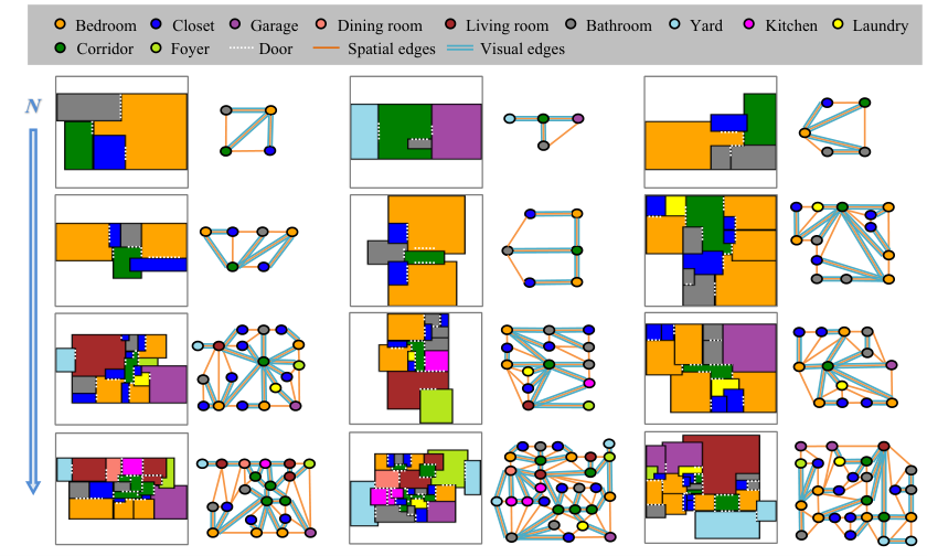
The Zillow Indoor Dataset (ZInD) cruz2021zillow contains 2,737 floorplans, from which we retrieved 1,217 and constructed graphs containing nodes and multi-relational edges. We show node and edge distributions in Fig. 9. The dataset includes different floorplans with a wide range of nodes and edges. We can see that most of the graphs have around 10 nodes; however, the most complicated floorplans contain around 30 rooms, 140 spatial edges, and 30 visual edges. We can also see that, in general, the number of spatial edges is 4-5 times more than that of visual edges. Some floorplan examples of the dataset are shown in Fig. 11.
Fig. 8 shows the frequency distribution of the room types. The dataset includes 17 different types of rooms. The top three most frequent labels are closet, bedroom, and bathroom. The top three least frequent labels are basement, breakfast nook, and dining room. In many cases, breakfast nooks are labeled as kitchens, and dining rooms are merged into living rooms, thus reducing the frequency of these two labels.


Name Value Basic room information room type ”bedroom” # of doors 1 # of windows 2 # of openings 0 Distance-based features room perimeter maximum length & width room area Shape descriptors chain code 03033133-1-1-1…-1 Image features panoramas features
A.2 Attribute extraction
Four types of attributes, including basic room information, distance-based features, shape descriptors, and image features, are extracted for each room. We concatenate features from different attribute sets and then feed them into the network. Detailed description of these attributes are listed in Table 10(b).
We use the Chain code freeman1961encoding to represent the shape of rooms. To generate a scale and rotation invariant shape descriptor, we first adopt the rule of 4-connected neighbourhood to traverse the boundary of the room, and record the direction of each step. As shown in Fig 10(a), we first choose a start position (i.e. (2,1)) and develop the chain code from it:
To make the chain code invariant to rotation, we compute the difference between elements in the code. So, each element can be computed as:
| (9) |
Then, we make the chain code invariant to start position by applying the minimum circular shift. Specifically, we rotating the elements in the chain code until it gives the smallest integer. From Fig 10(a), we can get and . Finally, we pad the chain code to a fixed length of 100 with -1.
Image features are extracted from a scene classification model using the NASNet model 22 2 https://www.tensorflow.org/api_docs/python/tf/keras/applications/nas net/NASNetMobile zoph2018learning followed by an average pooling layer and a fully connected layer for prediction. The features are extracted from the output of the last pooling layer and have a size of 1056. The classification model is pre-trained on ImageNet and then retrained on ZInD cruz2021zillow.


A.3 Graph construction
The floor plan can easily and naturally be represented as a graph. Each node represents a room, and edges represent the connectivity of two rooms. We construct graph edges by defining two types of edges, which are spatial edges and visual edges (Fig. 12). More samples of constructed graph are shown in Fig. 11.
Appendix B Implementation details
Our model has 2 iterative encoder blocks (). In each block, the graph attention layer applied on each subgraph has the dimension of 32. The three fully connected layers in decoder has the dimension of 64, 16, and 1, respectively. Adam optimizer is adopted to train the model, with a learning rate of that dropped 0.5 at and epochs. The model is trained for 300 epochs with early stopping. Implementation was done using PyTorch and trained with a Nvidia TITAN-XP GPU.
Appendix C Floorplan generation
We show more qualitative comparison of different graph structures (i.e. no edge given, kNN graphs, fully connected (FC) graphs, topology estimated by ITL) usage for floorplan generation. We show that ITL can generate effective and practical floorplan topological information, which leads to more realistic floorplan generation using HouseGAN nauata2020house. We can see that, without topological information (i.e. no edge provided), most of rooms in generated floorplan are separated. The kNN graph fails to provide compelling topology for HouseGAN, since it predicts connections based on the similarity of room attributes. Rooms generated with kNN graphs tend to be clustered by the room type (e.g. bedrooms are connected to bedrooms, closets are connected to closets). Furthermore, the fully connected graph will cause spatial overlap of rooms.
Appendix D Graph visualization
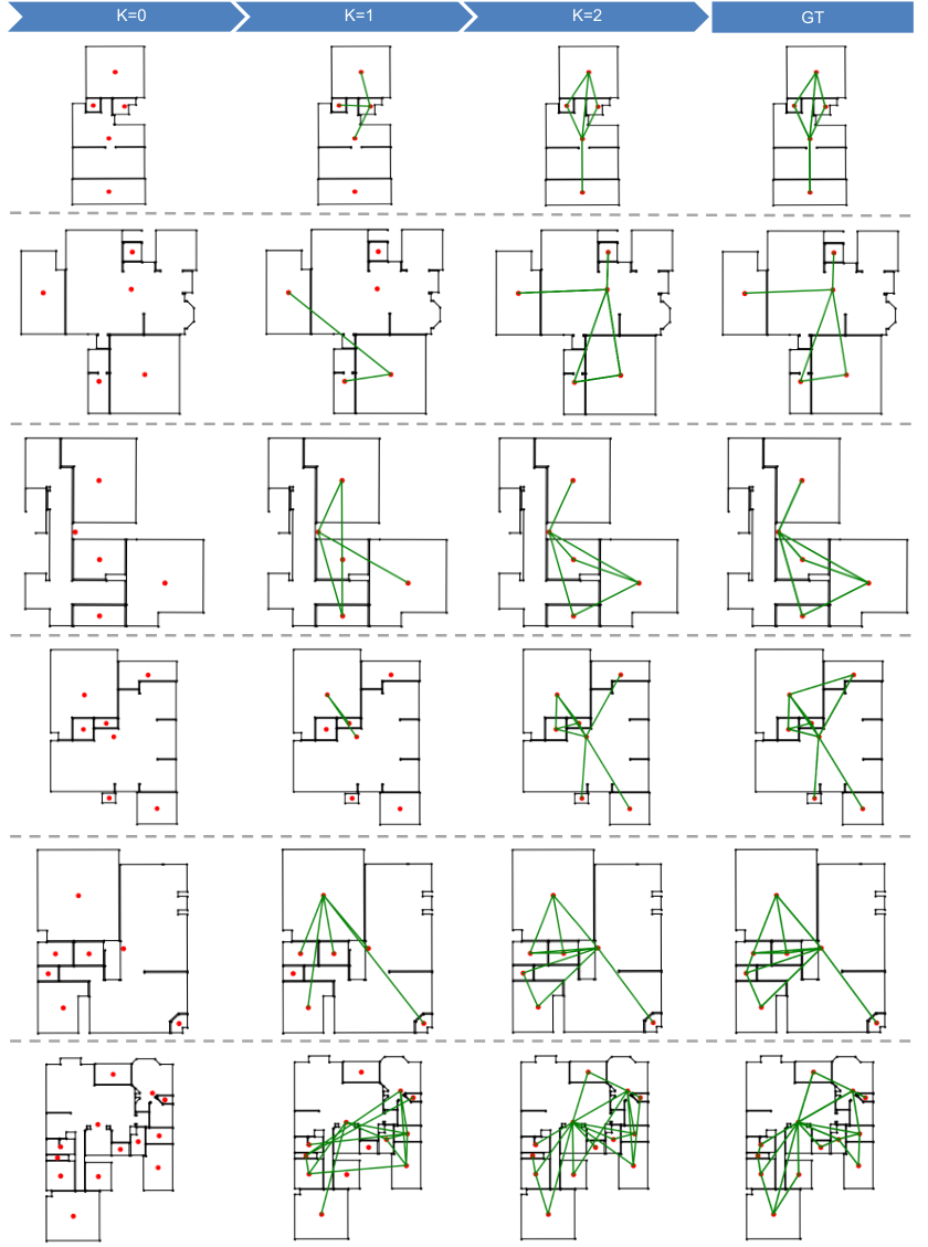
We visualize the learned graph topology in each iteration. As shown in Fig. 14, the initial graph topology is completely missing (i.e. ). After the first iteration (i.e. ), the model predicts a subset of the edges based only on node embeddings. Then the second iteration (i.e. ) will further refine the results and complement the predictions in the first iteration.
Appendix E Sensitivity analysis
We predict multiple types of edges (i.e. spatial and visual edges) in this work. We split spatial edges into two exclusive sets: door (i.e. visual) connectivity and wall connectivity, and then jointly predict all three types of edges by combining the loss function of each task. The loss function of the proposed model can be expressed as:
| (10) |
where , , and denote the binary cross-entropy loss for visual (door), wall, and spatial connectivity, respectively. and are two non-negative hyper-parameters in our model. We used in our paper.
To give more insight of the model, we conduct sensitivity analysis of these two hyper-parameters. Results are summarized in Table 6. We can see that the overall performance of the model is stable. When remains the same, a larger will improve the prediction performance for all types of edges. The improvement slows down if is greater than 1. When remains the same, a larger will lead to higher performance of the model. If is greater than 1, although the performance of door prediction is slightly improved, the performance of wall prediction will be greatly reduced, resulting in a decrease in overall performance.
Spatial Wall Door , 79.16 61.60 89.62 , 80.91 64.20 90.11 , 81.64 65.67 91.73 , 81.00 65.70 91.63 , 79.05 64.22 90.89 , 80.38 64.75 90.63 , 81.64 65.67 91.73 , 80.21 62.66 92.54
Appendix F Effect of long skip connection and weight sharing
Here, we demonstrate the effect of long skip connection in the proposed model. Table 7 shows the results with and without long skip connection. We set the initial room attributes (i.e. raw features) as the baseline and directly feed them into the decoder to predict multiple relationships between rooms. Then we remove the long skip connection in the proposed model, and predict edges using only learned features. Finally, we report results of using combined features (i.e. with long skip connection). The comparison of the raw, learned, and combined features are summarized in Table 7.
Note that in the proposed method, we do not share weights between blocks. iteration blocks are stacked together to give the final prediction. During our experiments, we found that not sharing weight gives us better performance (Table 7).
features Spatial Wall Door baseline raw 70.75 54.91 80.85 w/o long skip connection learned 75.64 60.66 90.37 ITL combined 81.64 65.67 91.73
Spatial Wall Door shared weights 72.38 60.99 87.13 different weights 81.64 65.67 91.73