Curvature loci of 3-manifoldsThanks: Work of R. Oset Sinha partially supported by Grant PGC2018-094889-B-100 funded by MCIN/AEI/ 10.13039/501100011033 and by “ERDF A way of making Europe”Thanks: Work of M.A.S.Ruas partially supported by FAPESP Proc. 2019/21181-0 and CNPq Proc. 305695/2019-3
Abstract.
We refine the affine classification of real nets of quadrics in order to obtain generic curvature loci of regular -manifolds in and singular corank -manifolds in . For this, we characterize the type of the curvature locus by the number and type of solutions of a system of equations given by 4 ternary cubics (which is a determinantal variety in some cases). We also study how singularities of the curvature locus of a regular 3-manifold can go to infinity when the manifold is projected orthogonally in a tangent direction.
Key words and phrases:
curvature locus, 3-manifolds, real nets of quadrics, Steiner Roman surface, second order geometry2000 Mathematics Subject Classification
Primary 57R45; Secondary 53A07, 58K051. Introduction
The extrinsic geometry of 3-manifolds in from a singularity theory viewpoint was investigated by M.C. Romero Fuster, R. Binotto and S. Costa in [3, 4] and by D. Dreibelbis in [7]. In the article [3], the authors study the behaviour of the curvature locus (also called curvature Veronese) of a 3-manifold immersed in describing the possible topological types at the different points of a 3-manifold immersed in Their work was motivated by [6], in which quadratically parameterizable surfaces, of which the Steiner surface is an example, have been studied in terms of their feasibility as surface patches in computer aided geometric design.
Motivated by the results in [3], the first and third authors, and A. Sacramento, introduced in [2], the invariants of the second fundamental form of corank 1 3-manifolds in and studied properties of its second order geometry in connection with the geometry of regular 3-manifolds in Notice that the image of the projection of a 3-dimensional smooth manifold into a hyperplane in along a tangent direction at a point gives (locally) a corank 1 3-manifold in a 5-dimensional space. The converse is also true, in other words, given a parametrized corank 1 3-manifold in defined in a sufficiently small neighbourhood of a point, there exists a 3-dimensional smooth surface in projecting onto it (See also [1]).
The aim of this paper is to complement these previous investigations, by presenting a more formal approach to the affine classification of the curvature locus of smooth and singular 3-manifolds in and respectively.
The affine geometry of the second fundamental form of a -dimensional manifold in is the study of invariants of the action of the affine group in the space of quadratic polynomial mappings Each such mapping generates a system of quadrics denominated a “net of quadrics”. One can find in the literature many texts about nets of quadrics (see [10, 11, 19, 20]).
We refine the affine classification of real nets of quadrics in order to obtain generic curvature loci of regular -manifolds in and singular corank -manifolds in . For this, we characterize the type of the curvature locus by the number and type of solutions of a system of equations given by 4 ternary cubics (which is a determinantal variety in some cases). We also study how singularities of the curvature locus of a regular 3-manifold can go to infinity when the manifold is projected orthogonally in a tangent direction.
The paper is organized as follows. In Sections 2.1 and 2.2, we review the definitions of first and second fundamental forms and the notion of curvature loci of regular and singular 3-dimensional manifolds in In Section 2.3, we present the affine classification of real nets of quadrics given by S. A. Edwards and C.T.C. Wall in [11]. From this section on, we restrict the discussion of the paper to 3-dimensional regular and singular manifolds in and respectively. The aim in Section 3, is to characterize the curvature locus, when this set is a substantial surface, that is, a surface with Gaussian curvature non identically zero. The main result in this section, is Theorem 3.1, in which we prove that the singular sets of the restriction of the second fundamental form to the unit sphere in are a complete set of invariants for the substantial curvature loci. The orthogonal projection of a regular 3-manifold in into along a tangent direction is a corank 1 3-manifold; their second fundamental form are the same, however their curvature loci are not equal. We discuss in Section 4 the relation between these two invariants. The goal in Section 5 is to prove Theorem 5.2, in which we classify the generic curvature locus of each -orbit of a quadratic map
2. Preliminary results
2.1. Second order geometry of -manifolds in
Given a smooth -dimensional manifold , and a local parametrisation of with an open subset, let be an orthonormal frame of such that at any , is a basis for and is a basis for at .
The second fundamental form of at a point is a symmetric bilinear map, given by , where is the canonical projection.
Furthermore, the second fundamental form of at along a normal vector field is the bilinear map given by .
For singular -dimensional manifolds with corank singularities, we shall need the following construction. Let be a corank -manifold in , , and consider a point . The singular manifold will be taken as the image of a smooth map , where is a smooth regular -dimensional manifold and is a corank point of such that . Also, consider a local coordinate system defined in an open neighbourhood of at . Hence, we may consider a local parametrisation of at (see the diagram below).
At the singular point the -dimensional tangent space , is given by , where is the differential map of at . Thus, the -dimensional normal space of at , , is the subspace orthogonal to satisfying .
The first fundamental form of at , is given by
The first fundamental form is not a Riemannian metric on , but a pseudometric instead. Let be the Cartesian coordinate system in . Taking the frame of , the coefficients of the first fundamental form of at with respect to are given by , , where .
Consider the orthogonal projection . The second fundamental form of at , in the basis of is given by , and we extend it to the whole space in a unique way as a symmetric bilinear map. Given a normal vector , we define the second fundamental form along , given by , for all .
2.2. The curvature loci
Given a -dimensional manifold , , the curvature locus at a point is the set . The curvature locus of a manifold contains all its second order geometry. Any isometric scalar invariant of the curvature locus is an isometric scalar invariant of the manifold since rotations in leave invariant the locus and rotations in rotate the locus. The contact geometry of the manifold is affine invariant. The curvature locus is not affine invariant, but the position with respect to the origin and, in some cases, the topological type are affine invariant.
Regular case:
For a regular manifold , the curvature locus is also the image of the map , where and is denoted by . The authors show in [3, p. 27] that taking spherical coordinates in , one can parametrise the curvature locus of at by , where
with
The first normal space is . The affine hull of the curvature locus is denoted by and the linear subspace of parallel to by . The curvature locus of a regular -manifold in can be seen as the image of the classical Veronese surface of order via a convenient linear map.
In [3, p. 34], it is shown that the curvature locus at a point where in a -manifold is isomorphic to one of the following: a Roman Steiner surface (Figure 4), a Cross-Cap surface (Figure 4), a Steiner surface of type (Figure 4), a Cross-Cup or type 6 surface (Figure 4), an ellipsoid, a (compact) cone or a planar region. The curvature locus at is said to be substantial if .


Singular case:
The curvature locus at a singular corank point of a -dimensional manifold , (denoted by ) is also given by the image of the map defined by , where is the subset of unit tangent vectors (i.e. vectors such that ).
Examples of topological types of for the case can be found in [2].
It is possible to take a coordinate system and make rotations in the target in order to obtain a local parmetrisation for at given by
where for . Hence the subset of unit tangent vectors is the cylinder given by
Taking an orthonormal frame of , the curvature locus can be parametrised by
where ,
are the coefficients of the second fundamental form with all the partial derivatives evaluated at , and are local coordinates of .
From now on we will focus in the cases of and . Notice that, locally (i.e. in neighbourhoods of the corresponding points), the latter can be obtained by an orthogonal projection in a tangent direction of the former. Notice too that the second fundamental forms coincide.
2.3. Real nets of quadrics
The affine geometry of the second fundamental form of a -dimensional manifold in is the study of invariants of the action of the affine group in the space of quadratic polynomial mappings . Each such mapping generates a system of quadrics denominated a “net of quadrics”. One can find in the literature many texts about nets of quadrics (see for instance [10, 11, 19, 20]). In [10] is presented a classification of the real nets of quadrics with respect to -equivalence (see [12] or [17] for the definition of the contact group and its action).
Let be the space of homogeneous polynomials of degree 2 in 3 variables. A net of quadrics is a system in generated by 3 polynomials , where for . Associated to each net there is a map germ , . Denote by the net given by , that is, . Let be the set of all nets . It follows from [11] that there is a Zariski open set of , denoted by , such that any net in can be taken in the form:
| (1) |
For quadratic polynomial mappings , this normal form is equivalent to the Hessian form
| (2) |
A net in this set is called a general real net of quadrics. As the normal forms of the generic nets are given by homogeneous polynomial maps of degree 2, and in this case, the corresponding map germ is 2-determined with respect to -equivalence, it follows that the -classification coincides with the classification by the action of the group .
The complete classification of quadratic mappings with respect to -equivalence can be found in [10, p. 315]. The family (1) is labelled , and according to the values of the parameters and . Table 1 presents the types , and its subcases. Type is given by , and the discriminant for cases and is .
The orbits in the complex case are labelled as follows:
| Name | |||||||||||||||
|---|---|---|---|---|---|---|---|---|---|---|---|---|---|---|---|
| Codimension | 0 | 1 | 1 | 2 | 2 | 2 | 3 | 3 | 3 | 3 | 4 | 4 | 5 | 7 | 7 |
The type depends on a modulus and in the real case it splits four subcases. Type , , , , , , and also have subcases.
The remaining cases are shown in Table 2, along with their respective discriminants.
| Name | Normal form | discriminant |
|---|---|---|
3. Curvature loci for regular -manifolds
The curvature locus is the image under a homogeneous quadratic map of the unitary tangent directions in , namely the image of . The group where and acts on the space of maps with the Whitney topology. If two maps and are -equivalent, their images are diffeomorphic. In a neighbourhood of a point in one can choose coordinates such that can locally be seen as a map from to . From the point of view of -equivalence the only stable singularity (stable under small perturbations) is the cross-cap (), for which we have a standard normal form given by
At a singular point we say that is finitely determined if there exists a positive integer such that for any with it follows that and are -equivalent at By the Mather-Gaffney criterion, a singularity is not finitely determined if it is not stable outside the point (see [13]).
In [6] the projective classification of quadratically parametrizable surfaces is given. Out of the surfaces studied there the compact ones are the possibilities for curvature loci of regular 3-manifolds, as pointed out in [3]. The description of these surfaces, given in [6] in a different terminology, is the following:
- (i)
The Roman Steiner surfaces has 6 cross-cap singularities (-points) joined in pairs by 3 transversal double point curves which intersect at a triple point.
- (ii)
- (iii)
The type 5 surface has 2 cross-caps joined by a transversal double point curve. One of these cross-caps lies on a tangent double point curve. The tangency of this double point curve is non-degenerate (the tangent sheets have different curvature) and the two end points of this curve are non finitely determined singularities. We shall call the two end points of the tangent double point curve -points (for tangent cross-cap).
- (iv)
The type 6 surface has no cross-caps. It has a tangent double point curve where the tangency is degenerate (the tangent sheets have the same curvature). The two end points of this curve are non finitely determined singularities. We shall call the two end points of the tangent double point curve -points (for degenerate tangent cross-cap).
Besides these, amongst the non-planar loci we have
- (v)
The truncated cone is a compact cone with a curve of singular points corresponding to the base of the cone and a singular point corresponding to the vertex of the cone. None of these singularities are finitely determined.
- (vi)
The ellipsoid has a curve of non finitely determined singular points.
From this classification it follows that the number and type of singularities of quadratically parametrised surfaces determine completely its equivalence class. It is also clear that generically one would expect to obtain a Roman Steiner surface or a Cross-cap surface. Besides this, following [6, 16], the -points and the -points (i.e. the non-finitely determined singularities of types 5 and 6) can be distinguished by the multiplicity of the double line in a neighbourhood of them, which is determined by intersecting the double line with transverse planes and resolving the singularity of the resulting curve by blowing up. We say that a self intersection is of multiplicity 1 if the two intersecting sheets are transverse, of multiplicity 2 if the sheets are tangent but have different curvature and of multiplicity 3 if the sheets are tangent and have the same curvature. With this notation, the cross-cap has multiplicity 1, the -points have multiplicity 2 and the -points have multiplicity 3.
The map is the restriction of the second fundamental form to , where and are the local coordinates of and of . The singularities of this restriction are captured by the zeros of the 3x3 minors of the following determinantal matrix. Given a local parametrisation in Monge form ( have zero linear and constant part) of where is the origin, define the matrix
The zeros of the 3x3 minors of this matrix, , are the solutions to a system of 4 homogeneous polynomials of degree 3 in 3 variables, i.e. 4 ternary cubics. The first one of these equations is the determinant of the 3x3 minor given by the 3 first rows of and is the determinant of the Jacobian matrix of the second fundamental form, which we call . This first equation is precisely the equation to obtain the asymptotic directions (see [7]). We call , the determinant of the remaining 3 minors, where is the row of removed. The solution to this system is a homogeneous algebraic variety which is generically a collection of lines passing through the origin. These solutions have a certain multiplicity defined by the number of points of the intersection of the line with a generic plane away from the origin. The intersection of these lines with correspond to the singularities of the curvature locus, so we have the following characterisation.
Theorem 3.1.
Suppose is parametrised by in Monge form and suppose that it has a substantial (i.e. non-planar) curvature locus . Then
- (i)
is a Roman Steiner surface if and only if is 6 real lines of multiplicity 1.
- (ii)
is a Cross-cap surface if and only if is 2 real lines and 4 complex lines of multiplicity 1.
- (iii)
is a type 5 surface if and only if is 4 real lines, two of them with multiplicity 2 and 2 with multiplicity 1.
- (iv)
is a type 6 surface if and only if is 2 real lines of multiplicity 3 each.
- (v)
is a truncated cone if and only if has a plane and a real line as the only real solutions and (possibly) some complex solutions.
- (vi)
is an ellipsoid if and only if has a plane as the only real solution and (possibly) some complex solutions.
Proof.
This follows from the description of the types of locus and their singularities and the relation between the multiplicity of the singular points in the locus defined above and the multiplicity of the solutions in . Items i) to iv) are a consequence of the following fact: the complexification of is the representation matrix of a codimension 2 Cohen-Macaulay determinantal singularity in (see [9], [8]). The equations defining the minors of are homogeneous of degree 3, so the ideal defined by has multiplicity 6 (see Lemma 5.5 in [5]) (i.e. the homogeneous curve intersects in 6 points a plane away from the origin) and the sum of the multiplicities of the solutions to the system must be 6. A solution to this system is generically a real line with multiplicity 1. On the other hand, in the curvature locus a singularity is generically a cross-cap. This means that the real lines of multiplicity 1 correspond to -points, i.e. the multiplicity of the solution to the system coincides with the multiplicity defined for -points.
Now, if we deform a -point, two -points appear generically. By conservation of number, this means that the -points correspond to solutions of multiplicity 2. Similarly, the -points deform into three -points, and so -points correspond to real lines of multiplicity 3 as solution to the system. Taking into account the multiplicities of the singular points for each type of locus and that the sum of the multiplicities must be 6, the only possibilities are as in the statement.
For items (v) and (vi) is not a determinantal variety since there are mixed dimensions and the multiplicity is not well defined. ∎
Remark 3.2.
There is a natural equivalence when working with singularities of matrices. The group where is changes of coordinates in the source and acts naturally by multiplication to the left and to the right on the matrices. If two matrices and are -equivalent, then and are isomorphic, where stands for the zeroes of the minors. This means that inside a certain -orbit, the affine type of curvature locus of the associated 3-manifold does not change.
However, two parametrisations of regular 3-manifolds whose associated matrices and are -equivalent, may have associated nets of quadrics in different affine -orbits, as examples (iii) and (iv) below show.
Example 3.3.
Consider given by , a local parametrisation at the origin in a Monge form, as before.
- (i)
Let be its second fundamental form at . The 3x3 minors of are , , and . Hence, the solution of , is given by , . Take the solution , and consider the plane , which is transverse to the line. The algebraic multiplicity of this line is given by replacing by 1 and evaluating in the dimension of the local algebra , where is the local ring of functions in 3 variables. Hence, we obtain multiplicity 1 in this case. Similarly, the first two solutions have multiplicity 2 and correspond to -points and the last two solutions correspond to the cross-cap points. Here is a type 5 surface.
- (ii)
Now, let be such that the second fundamental form at is given by . For this case, , , and . There are two solutions for , : , . Both of these solutions have multiplicity 3 and correspond to -points. Here is a type 6 surface.
- (iii)
Taking as the second fundamental form at , , , and . Thus, the solution of , , is , . Notice that the solution is a plane and a line. The curvature locus is a truncated cone. The associated net of quadrics lies in orbit from Table 2.
- (iv)
Finally, let . For this example, , , and . Therefore , , that is, a plane and a line and is also a truncated cone. Here the associated net of quadrics lies in orbit from Table 2.
Remark 3.4.
As a corollary of this theorem we get certain implications about the solutions of the system of 4 ternary cubics described above. For example, the fact that there is always a real solution means that at least one of the four minors must be a reducible equation. We can also see that the complex solutions cannot have multiplicity 2, as that would imply that one of the minors is a degree 4 polynomial (complex solutions come together with their conjugate solutions) and therefore would not be a cubic.
This characterisation of the topological types of non-planar curvature loci allows us to obtain sufficient geometrical conditions in order to have a certain topological type.
Proposition 3.5.
Let the curvature locus of at be parametrised by , where
with
If (i.e. ) and are linearly independent, then the curvature locus is a Roman Steiner surface.
Proof.
Let , and . Call . We have . Since , to calculate or must be zero. Suppose , then
Notice that implies that at most 3 2x2 minors can have 0 determinant, so at most one of the above equations vanishes. Therefore, the only solution different from is .
Similarly when or . Therefore is 6 real lines whose intersection with is the 6 cross-caps of the Roman Steiner surface. ∎
4. Curvature loci for singular 3-manifolds
Projecting orthogonally a regular 3-manifold in along a tangent direction yields a singular 3-manifold in . The second fundamental form is the same in both cases. However, the curvature locus is different since the unitary tangent vectors form an in the regular case and the cylinder in the singular case.
In [1, p. 402] asymptotic directions for are defined and studied, in particular, the authors show that a direction is asymptotic if and only if the determinant of the Jacobian of the second fundamental form vanishes. They also show that, similarly to the regular case ([7, p. 451]), the singular points of the curvature locus correspond to the image of asymptotic directions by the second fundamental form. Furthermore, they show that when you project orthogonally a regular 3-manifold in along an asymptotic direction this direction becomes an infinite asymptotic direction of the singular 3-manifold in . This suggests that when you consider seen as the projection of , the number of singularities of the curvature locus will depend on whether the direction of projection is asymptotic or not. Our goal in this section is to understand this situation.
Consider where . Changing the last row of by the partials of we get a determinantal matrix which we call . The singularities of the curvature locus of a singular 3-manifold are controlled by . We call the determinants of the minors of and , . We use the superscript for the determinants in the regular case. Notice that .
In contrast with the regular case, the classification of the topological types of curvature loci for singular 3-manifolds in seems very hard to tackle as the following examples illustrate. Consider given by , a local parametrisation at the origin in a Monge form. We shall project along different tangent directions to showcase the possibilities for the curvature locus of the projected singular 3-manifold at the origin.
Example 4.1.
Let be the second fundamental form of at . The curvature locus at the origin is a Roman Steiner surface, since is 6 real lines. Consider the asymptotic direction , whose image by is the triple point (hence it is not a cross-cap point). The curvature locus at the origin of obtained by orthogonally projecting along is given by , a surface with two cross-cap points (there are 3 solutions in , one being the -axis, the null tangent direction) that is shown in Figure 5 (left). Using the same map , we shall project along , an asymptotic direction whose image is a cross-cap. In order to do so, we make a rotation in the source, taking to , so that . Hence, has six solutions, one being the -axis and the curvature locus at the origin is a surface with five cross-caps points, as seen in Figure 5 (center). Still considering and projection along , an asymptotic direction whose image lies in a double point curve, we obtain again six solutions in , one being the -axis. Again, the curvature locus has five cross-caps (see Figure 5, right). Rotations in the source are also applied to take to , and we obtain .
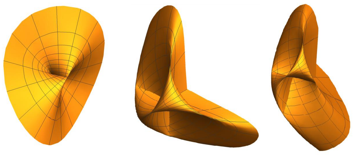
Example 4.2.
Consider as the second fundamental form of at . The curvature locus at is a Roman Steiner surface, but this time the -axis is not an asymptotic direction. Projecting along , has six solutions, none of them being the -axis, which means that the curvature locus at the origin of the singular 3-manifold has six cross-caps and it is parametrised by . Finally, we will project along , whose image is the triple point of the curvature locus. Rotating the source to take to , we obtain . In this case, has five solutions, one of them being the -axis. Therefore, the curvature locus at the origin has four cross-caps.
Theorem 4.3.
Consider and its projection along a tangent direction . Suppose that the direction of projection is not asymptotic. Then is isomorphic to . In particular, the curvature loci of and have the same number and type of singularities.
Proof.
For simplicity we consider the direction of projection to be since by rotation in the tangent space we can take any other direction to . Express the 2-jet of the parametrisation of the singular 3-manifold as
where are homogeneous degree 2 polynomials in . Evaluating the Jacobian of the second fundamental form on we get the matrix
If is not asymptotic, then . By Proposition 5.2 in [2] if then, by linear changes of coordinates in the target, the 2-jet of the parametrisation can be taken to
with and such that is -equivalent to one of the orbits or . We consider now the matrix
Using from the group we can do operations with the lines of to obtain a matrix which differs from only in the last line, where we get . Doing the change of coordinates we obtain a matrix such that is isomorphic to . Notice that gives the singular set of a map restricted to the cylinder where is composed with the previous change of coordinates in the source. This change of coordinates does not affect the corresponding image, therefore, is ismorphic and so is isomorphic to . ∎
Proposition 4.4.
Suppose the direction of projection is an asymptotic direction, then the curvature locus of the singular manifold has at least one singularity less than the locus of the regular manifold. In particular, if the direction of projection corresponds to a cross-cap singularity, this cross-cap goes to infinity in the locus of the singular manifold.
Proof.
If is asymptotic then and so . On the other hand is
and so for some functions . So for . This means that is a solution in but since it does not intersect the cylinder this singularity lies at infinity. ∎
5. The generic curvature locus of a -manifold
Finding necessary and sufficient conditions in terms of geometric invariants to characterize the topological type of the curvature locus at a given point of a -manifold seems to be a hard task.
The curvature locus being substantial or not is affine invariant but its topological type is not affine invariant for 3-manifolds. Our goal in this section is to classify the generic curvature locus of each -orbit of a quadratic map
More precisely, with the notation of Section 2.3, given a net , we can naturally associate the -jet of parametrisation of a smooth -manifold in the Monge form:
whose second fundamental form at the origin is given by the quadratic map . The curvature locus of a normal form in Tables 1 and 2 are not generic in general from the geometrical point of view. Constructing with those normal forms and where may not give the best possible situation.
The classification of -orbits can be refined by the -classification of the matrices corresponding to the nets in each -orbit.
Consider a generic positive definite homogeneous map ,
| (3) |
Our aim is to obtain a linear map such that the following diagram commutes
Changing for in the associated determinantal matrix we get
Proposition 5.1.
The generic normal form (in the sense of the -classification) of the net is given by and the singularities of the generic curvature locus are given by .
Now we can obtain the generic curvature locus in each -orbit.
Theorem 5.2.
Let be a net of quadrics and
a parametrization of whose second fundamental form at the origin is . Then, for each possible -orbit of , Table 3 provides the generic curvature locus of at the origin.
| Curvature locus | -Orbit |
|---|---|
| Roman Steiner | |
| Cross-cap | |
| Type | |
| Type | |
| Cone | |
| Ellipsoid |
Proof.
Consider such that is in one of the first -orbits: , or . Thus,
To determine the generic topological type of the curvature locus, we must investigate the number of singular points of when restricted to the unit sphere. In order to do so we calculate the -minors of the matrix
Since we are only interested in the number of singular points, linear changes in do not interfere. Hence, after linear changes, we can rewrite as
The -minors of are
Let . Then or . If , we have two solutions for , . If , this equation has 0,1 or 2 solutions according to the sign of : positive, zero or negative, respectively. It is possible to show that if , we have four solutions of , whenever and two solutions if and . Taking ,
The equation may have 1 or 2 solutions, since its discriminant . This discriminant is represented by a pair of coincident lines in the plane . Therefore, , have 4 solutions if and 2 if .
Each one of the orbits , and intersects a region of the plane where and , hence every orbit have generically six singular points and, therefore, the associated -manifold has, at the origin, a Roman Steiner surface as its curvature locus. Also, the orbits , and intersect regions of the plane where and , where two real and four complex solutions can be found. Hence in those orbits and the curvature locus can be a cross-cap surface as well. See Figure 6.
The remaining cases are similar. However, we need Proposition 5.1. Consider for example the orbit in Table 2, given by . The matrix of restricted to is
where is as in (3). Calculating the minors , , we obtain six solutions for when , four solutions when and two solutions otherwise. Hence, we may obtain a Roman Steiner surface, Type 5 or a Cross-cap as the curvature locus of the associated -manifold at the origin, respectively. The generic cases, however are the Roman Steiner and the cross-cap. In order to obtain a Roman Steiner surface as a generic curvature locus, for example, we may consider , , and . Hence , and the normal form of the net is given by . ∎
In fact, applying Proposition 5.1 to each normal form we get
Corollary 5.3.
For each orbit in Table 2, Table 4 shows a normal form of the net for which we obtain the generic curvature locus of the associated -manifold.
| Name | Normal form |
|---|---|
| (Roman Steiner) | |
| (Cross-cap) | |
| (Roman Steiner) | |
| (Cross-cap) | |
| (Steiner Romana) | |
| (Cross-cap) | |
| , | |
| (Cross-cap) | |
We can also deduce the generic curvature locus for the same -orbits but for singular manifolds.
Corollary 5.4.
Let be a net of quadrics and
a parametrization of whose second fundamental form at the origin is . Then, for each possible -orbit of , Table 5 provides the generic curvature locus of at the origin.
| Curvature locus | -Orbit |
|---|---|
| 6 CC | |
| 2 CC | |
| 2 CC and 2 TCC | |
| 2 DTCC | |
| Ellipse | |
| Paraboloid |
Proof.
For all -orbits except for , there exists a non-asymptotic direction in . In this case, if we take the normal form which yields the generic curvature locus as in Table 4 and project in a non-asymptotic direction, by Theorem 4.3, the curvature locus of the singular projection will have the same number and type of singularities as the curvature locus in the regular case. In most cases (all orbits except for , , , ) is an asymptotic direction, so we must chose a different direction to do the projection. This projection will force a linear change of coordinates in the tangent space which will eventually force a linear change of coordinates in the source in the normal forms of Table 4. However, this change of coordinates lies in and so we do not change the type of -orbit. For all, except for the above mentioned 4 orbits, the generic normal form will change.
For the orbit , all tangent directions are asymptotic so the number and type of singularities of a generic curvature locus in this orbit for the singular case will change. Notice that any singular 3-manifold with the associated net in this -orbit will have a parametrisation -equivalent to . This means that the 2-jet depends only on and and so the generic curvature locus in this orbit is an ellipse. ∎
References
- [1] P. Benedini Riul and R.Oset Sinha Relating second order geometry of manifolds through projections and normal sections. Publ. Mat., v. 65 (2021), n. 1, p. 389-407.
- [2] P. Benedini Riul, M. A. S. Ruas and A. de Jesus Sacramento Singular 3-manifolds in . Rev. R. Acad. Cienc. Exactas Fís. Nat. Ser. A Mat. RACSAM 116, 56 (2022), n. 1, 18 pp.
- [3] R. R. Binotto, S. I. Costa and M. C. Romero Fuster The curvature Veronese of a -manifold in Euclidean space. Real and complex singularities: Amer. Math. Soc., Providence, RI (2016), (Contemp. Math., v. 675), p. 25–44.
- [4] R. R. Binotto, S. I. Costa and M. C. Romero FusterGeometry of 3-manifolds in Euclidean space.In: Theory of singularities of smooth mappings and around it. Res. Inst. Math. Sci. (RIMS), Kyoto, (RIMS Kôkyûroku Bessatsu, B55) (2016) p. 1–15.
- [5] C. Bivià-Ausina and J.J. Nuño-Ballesteros Multiplicity of iterated Jacobian extensions of weighted homogeneous map germs. Hokkaido Math. J. 29 (2000), no. 2, 341–368.
- [6] Coffman, A., Schwartz, A. J. and Stanton, C. The algebra and geometry of Steiner and other quadratically parametrizable surfaces. Computer Aided Geometric Design, 13(3), 257-286. (1996).
- [7] D. Dreibelbis Self-conjugate vectors of immersed 3-manifolds in . Topology Appl. 159 (2012), no. 2, 450–456.
- [8] A. Frühbis-Krüger Classification of simple space curve singularities. Comm. Algebra 27 (1999), no. 8, 3993–4013.
- [9] A. Frḧbis-Krüger and A. Neumer Simple Cohen-Macaulay codimension 2 singularities. Comm. Algebra 38 (2010), no. 2, 454–495.
- [10] du Plessis, A. and Wall, C. T. C. The geometry of topological stability. London Mathematical Society Monographs. New Series, 9. Oxford Science Publications. The Clarendon Press, Oxford University Press, New York, viii+572 pp. (1995).
- [11] Edwards, S. A. and Wall, C. T. C. Nets of quadrics and deformations of singularities. In Mathematical Proceedings of the Cambridge Philosophical Society. Cambridge University Press, 105 (1), 109-115. (1989).
- [12] Mather, J. N. Stability of mappings, IV: Classification of stable map-germs by -algebras. Publications Mathmatiques de l’Institut des Hautes tudes Scientifiques, 37(1), 223-248. (1969).
- [13] D. Mond and J.J.Nuño-Ballesteros, Singularities of Mappings, Grundlehren der mathematischen Wissenschaften, No. 357 Springer, (2019).
- [14] J. J. Nuño-Ballesteros and F. Tari, Surfaces in and their projections to -spaces. Proc. Roy. Soc. Edinburgh Sect. A, 137 (2007), 1313–1328.
- [15] R. Oset Sinha and F. Tari, Projections of surfaces in to and the geometry of their singular images. Rev. Mat. Iberoam. 32 (2015), no. 1, 33–50.
- [16] M. Reid Undergraduate algebraic geometry. Cambridge University Press, (1988).
- [17] Wall, C. T. C. Finite Determinacy of Smooth Map-Germs. Bulletin of the London Mathematical Society, 13(6), 481-539. (1981).
- [18] Wall, C. T. C. Nets of conics. Mathematical Proceedings of the Cambridge Philosophical Society. Cambridge University Press, 81(3), 351-364. (1977).
- [19] Wall, C. T. C. Nets of quadrics, and theta-characteristics of singular curves. Philosophical Transactions for the Royal Society of London. Series A, Mathematical and Physical Sciences, 229-269. (1978).
- [20] Wall, C. T. C. Singularities of nets of quadrics. Compositio Mathematica, 42(2), 187-212. (1980).