Effects of attractive inter-particle interaction on cross-transport coefficient between mass and heat in binary fluids
Abstract
In some binary fluids, mass transport is observed under a temperature gradient. This phenomenon is called the Soret effect. In this study, we discuss the influence of inter-particle interaction. We considered equimolar binary Lennard-Jones fluids with a mass contrast, whereas the interaction was common for all the particle pairs with various cut-off lengths. We performed molecular dynamics simulations of such fluids under equilibrium to obtain the cross-transport coefficients between the fluxes of mass and heat. The simulation revealed that this quantity strongly depends on the cut-off length. Further, we decomposed the heat flux into kinetic and potential contributions and calculated the cross-correlations between decomposed fluxes and the mass flux. The result indicates that the potential contribution dominates , implying that the Soret coefficient is altered by the inter-particle interaction.
I Introduction
A concentration gradient is induced by a temperature gradient for some binary mixtures of fluids due to the mass transferplatten. This phenomenon is the so-called thermodiffusion or the Ludwig-Soret effect being characterized by the Soret coefficient defined as follows.
| (1) |
Here, is the mutual diffusion coefficient and is the thermal diffusion coefficient. One of the fluids moves to the cold side when is positive, whereas it moves to the hot side when is negative.
For binary gases, the mechanism of the Soret effect has been theoretically clarified. Chapman and Enskogchapman theoretically described for dilute gas mixtures according to the rigid body collisions. The theory has been experimentally verified for and , and and mixtures by Chapman and DootsonDootson, Blüh et al.bluh, and Ibbs et al.Ibbs
In contrast, for liquid mixtures, the mechanism of the phenomenon has not been fully clarified yet, even for simple systems due to the strong correlation between the constitutionswirtz. The earliest experimental report was made for various salt solutionssnowdon1960, and studies for the other systems followed. For instance, TannerTanner; Tanner1, Prigogine et al.Prigogine.1952; Prigogine.1950 and Saxton et al.Saxton reported the results for organic liquids. Korsching et al.korsching performed a series of experiments on isotope separation. Various theoretical models have been proposed to explain these experimental data of the Soret coefficients. Thermodynamic and phenomenological models have been developed. In such phenomenological modelsDenbigh; Hartmann; Hartmann2; Keshawa; Morozov; haase; Kempers; Wurger; Dougherty; Morteza, the Soret coefficient is related to the macroscopic thermodynamic quantities such as the heat of transport and the molar enthalpy.
Molecular dynamics (MD) simulations are useful to investigate the Soret coefficients of liquids directlykohler; artola. In MD simulations, roughly there are two different methods to calculate the Soret coefficient. One is the non-equilibrium MD (NEMD) simulation method, in which a temperature gradient is applied to the system. Non-equilibrium physical quantities such as the heat flow can be directly calculated in a NEMD simulation, and the Soret coefficient can be estimated without phenomenological assumptions. To calculate the heat flow efficiently, we can utilize the reverse NEMD (RNEMD) methodReith; Galliero1; Galliero2. In the RNEMD method, the heat flow is imposed to the system and the temperature gradient is measured. With this method, we can avoid the statistically inefficient calculation of the heat flow. Reith and Müller-Plathe Reith, and Galliero et al Galliero1; Galliero2 utilized the RNEMD method to calculate the Soret coefficient of binary LJ liquids. Another is the equilibrium MD (EMD) method. In this approach, the Soret coefficient is obtained from the linear response theory in equilibriumD.todd. According to the linear response theory, transport coefficients can generally be calculated from a correlation function of the fluctuations of the flux at equilibrium. For instance, Sarman and EvansSarman reported that the EMD reproduces the consistent results with NEMD. Hoheisel and VogelsangVogelsang1988 conducted a systematic study to report that particles with larger mass and larger cohesive energy move to the cold side. Vogelsang et al.Vogelsang1987 introduced an interesting analysis method which utilizes the decomposition of fluxes. They decomposed the heat flux into kinetic, potential and enthalpy contributions to report that the enthalpy contribution is dominant in the thermal diffusion coefficient (and thus in the Soret coefficient). However, they presented the result only for a specific interaction that mimics Ar-Kr mixtures.
Motivated by the work by Vogelsang et al, in this work we studied the contributions of different heat flux components to the transport coefficient. We employed equimolar binary liquid mixtures which have the constant mass ratio and similar liquid structures but different interaction potentials. By changing the inter-particle interaction systematically, the dynamic properties can be changed while the static liquid structure is almost unchanged. We decomposed the heat flux into the kinetic and potential contributions, and calculated the cross-correlation functions for the mass flux and the decomposed heat fluxes. Based on the cross-correlation functions, we discuss which contribution is sensitive to the inter-particle potential. Details are shown below.
II Model and Analysis
To provide a strategy of analysis, before presenting simulation details, let us consider a macroscopic non-equilibrium three-dimensional system where several fluxes are induced by thermodynamic forces. To discriminate the different fluxes, we use the subscript and express the -th macroscopic flux as . We express the thermodynamic force, which is conjugate to the -th flux as . The fluxes at a given position and a given time are generally given as functionals of the thermodynamic force as
| (2) |
If the system is near equilibrium and the spatial and temporal variation of the fluxes are broad and slow, Eq. (2) can be phenomenologically rewritten as
| (3) |
where are Onsager coefficients, which are second-rank polar tensor.
To study the Soret effect, we consider binary mixtures of fluids. As the fluxes, we consider the mass flux of particles 1 , the mass flux of particles 2 and the heat flux . To satisfy the momentum conservation, . Then Eq. (3) can be rewritten as the following set of equations:
| (4) | ||||
| (5) |
From the viewpoint of the transport phenomena, the mass and heat fluxes can be expressed phenomenologically in terms of the gradients of the temperature field and the volume fraction fieldD.todd.
| (6) | ||||
| (7) |
where is the gradient of temperature, is the gradient of volume fraction of particle 1, is the Dufour coefficient, is the thermal conductivity, is the mass density, and is the chemical potential of particle 1. By comparing Eqs. (4) and (6), and can be written asD.todd
| (8) | ||||
| (9) |
The Soret coefficient can be obtained from and according to Eq. (1). To calculate , we need to obtain . Acquisition of chemical potential by EMD is generally difficult. In this work, we discuss instead of the Soret effect. Indeed, has the same sign as (as far as is positive), and can be calculated accurately. We limit ourselves to simple systems where .
Meanwhile, in our EMD simulations, we consider equimolar binary mixtures of fluids, for which the mass of the particle 1 is and the mass of the particle 2 is . The inter-particle interaction is common for all the particle pairs in the system, and it is written as follows:
| (10) |
Here, is the distance between two particles, is the particle size and is the intensity parameter. is the potential shift to attain at . We chose units of length, energy and mass as , , and . Namely, for the case with , we have an attractive part, whereas with the interaction is purely repulsive. The static liquid structure, which can be characterized by the radial distribution function, was not sensitive to the value of in the examined parameter range. We performed the EMD simulations with particles with the density at , the mixing ratio at , the mass ratio at , and the normalized temperature defined as at to minimize the fluctuations of macroscopic fluxesSmit. The equations of motion were integrated with the velocity Verlet algorithmComputer in LAMMPSLammps, and the integration step size was . and were fixed at unity. We performed simulations with steps (). Before the data acquisition, we set the temperature as by using Nosé-Hoover thermostat. To equilibrate the system sufficiently, we performed simulations with steps () before the data acquisition.
The Onsager coefficients can be calculated from the correlation functions calculated in the EMD simulations. The linear response theoryD.todd relates the correlation functions to the Onsager coefficients. We expect that the simulation box is much smaller than the characteristic length scale of the macroscopic fields. Then the Onsager coefficients are calculated by using the correlation function of the integrated total fluxes in a simulation box. The mass flux of the MD system is expressed as follows, in terms of the microscopic state:
| (11) |
where is the mass of the -th particle, is the number of particle 1 and is the velocity of the -th particle at time . However, the microscopic heat flux is not simple and there are different expressions for the microscopic heat flux. In this study, we employ the Irving and KirkwoodIrving1950 expression for by interpreting the heat flux as the energy flux:
| (12) |
where is the position of the -th particle at time , and is the total number of particles. The Onsager coefficients and can be expressed in terms of the equilibrium correlation functions as followsD.todd:
| (13) | |||
| (14) |
Here, represents the equilibrium statistical average, is the volume. Note that and are microscopically defined and they fluctuates with time. We multiply the factor of because the system is isotropic. This integral is evaluated by the trapezoidal rule after equilibrium molecular dynamics simulations.
III Results
Figures 1 and 2 show and as functions of the cut-off length of the potential. Note that the magnitude of statistical error is smaller than the symbol in the plots. Figure 1 demonstrates that decreases with increasing at , it shows a minimum around and approaches to a steady value in . shown in Fig. 2 also decreases with increasing . However, it monotonically decreases without showing any minima within the examined range. Further, goes down to negative around . This change in corresponds to the change of sign for . As we stated, the positive for small means that the lighter particles migrate toward the low-temperature side. When the sign of changes with increasing , the lighter particles move to the opposite direction.


To analyze the change of induced by , we observe the cross-correlation function defined as . Figure 3 shows for various . In the case of small , monotonically decays with time. As increases, gradually exhibits an undershoot, and the magnitude of undershoot increases. As a result of this undershoot, becomes negative, and it causes a negative in Fig. 2.

To see the origin of the undershoot in , we decompose the energy flux into the kinetic and potential contributions ( and , respectively) as shown below:
| (15) |
| (16) |
| (17) |
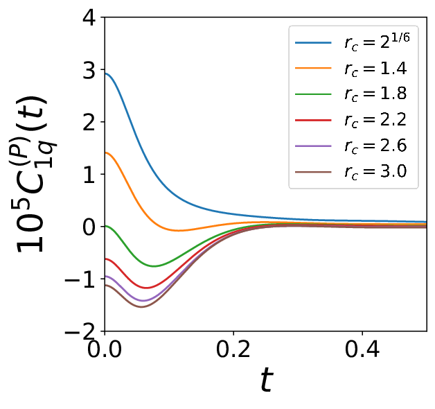
For the flux given in Eqs. (16) and (17), we calculated the cross-correlation functions and

|
Figure 4 shows the cross-correlation functions thus calculated, demonstrating that the kinetic contribution is not sensitive to . Here, we should stress that the insensitivity of to is not trivial. As we explained, the fluid structure is not sensitive to , but the dynamical properties such as the diffusion coefficient generally depend on . In contrast, the potential contribution is significantly dependent on . These results clearly demonstrate that the interaction dependence of shown in Fig. 2 comes from . In particular, the negative is due to the undershoot in in .
IV DISCUSSIONS
We note that the results may be altered if a different heat flux expression is employed. For instance, Hoheisel and Vogelsang Vogelsang1988 employed the Bearman-Kirkwood expressionMacgowan1986; onuki shown below:
| (18) |
where is the molar enthalpy of particles . Using this heat flux, they obtained for a soft-core system and reported that the sign of is negative. This result contradicts our results in Fig. 2 at . Namely, Eq. (18) employs , which is not straightforwardly obtained from microscopic simulations. We note that temperature and potential are also different from ours, although the effect seems not significant. This inconsistency is due to the expression of the heat flux.
We also note that Sasasasa has recently proposed the other expression of the heat flux as written below:
| (19) |
where , and , are the energy density flux, the energy density and the momentum density in the moving frame with the local velocity. These quantities should be defined in the moving frame since the contribution of the local velocity should be subtracted. is the mass density and is the thermodynamic pressure derived from the local thermodynamic entropy. Eq.(19) has a rigid microscopic origin, obtained from the Hamiltonian dynamics and local equilibrium assumptions for a chosen coarse-grained length scale. However, this heat flux is not easily obtained from the trajectories in EMD simulations.
We also note that Sasa theory includes a physical quantity corresponding to the molar enthalpy like Bearman-Kirkwood. Therefore, in order to correctly describe the macroscopic transport, the contribution of molar enthalpy must also be taken into account. However, even if the molar enthalpy contribution is added, the expressions for the kinetic energy and potential energy contributions for the heat flux remains the same. If the correct heat flux with the enthalpy contribution is employed, we have the third cross-correlation function for the enthalpy flux. The difference between our results and that by Hoheisel and VogelsangVogelsang1988 means that the enthalpy flux has so strong a contribution that the sign of the transport coefficient is changed. As future studies, it is demanding to obtain the cross-correlation function for the enthalpy flux in our system. Then we will be able to study how different correlation functions affect the transport coefficient and which one is dominant.
V Conclusions
To see the contributions of kinetic and potential origins in the heat flux to the transport coefficient , we conducted molecular dynamics simulations for equimolar binary fluids with the inter-particle potential of various cut-off lengths . The simulation revealed that changes its sign by . Specifically, for the case with , whereas for small . We decomposed the heat flux into the kinetic and potential contributions, and calculated the cross-correlation functions between the mass flux and the decomposed heat fluxes. The result demonstrated that the sign of is dominated by the potential contribution.
It would be fair to mention that our results may be changed if other expressions for the heat flux are employed instead of the Irving-Kirkwood heat flux. Although the Irving-Kirkwood heat flux is not thermodynamically correct, our cross-correlation functions for the kinetic and potential energy fluxes are correct. We expect that how these cross-correlation functions depend on the cutoff provides useful information to discuss the cross-transport coefficient with the enthalpy contribution. The calculations of with different expressions of the heat flux including the statistical mechanically correct expression by Sasasasa will be required. It would be an interesting and important future work.
VI Acknowledgment
The authors thank Prof. Sasa (Kyoto University) for informing his work on the derivation of hydrodynamic equations from the Hamiltonian dynamics.
References
- (1) J. K. Platten, Journal of Applied Mechanics 73, 5 (2006).
- (2) S. Chapman, and T. G. Cowling, The Mathematical Theory of Non-uniform Gases (Cambridge University Press, Cambridge, 1970).
- (3) S. Chapman and F. W. Dootson, Philos. Mag. 33, 248 (1917).
- (4) G. Blüh, O. Blüh, and M. Puschner, Philos. Mag. 24, 1103 (1937).
- (5) T. S. Ibbs, Roy. Soc. Proc. 93, 148 (1916)
- (6) P. N. Snowdon and J. C. R. Turner, Trans. Faraday Soc. 56, 1812 (1960).
- (7) C. C. Tanner, Trans. Faraday Soc. 23, 75 (1927).
- (8) C. C. Tanner, Trans. Faraday Soc. 49, 611 (1953).
- (9) I.Prigogine, L. Brouckere, and R. Buess, Physica 18, 915 (1952).
- (10) I.Prigogine, L. Brouckere, and R. Amand, Physica 16, 851 (1950).
- (11) R. L. Saxton, E. L. Dougherty, and H. G. Drickamer, J. Chem. Phys. 22, 1166 (1954).
- (12) H. Korsching, Naturwissenschaften 31, 348 (1943).
- (13) K. Wirtz, Z. Naturforsch 3a, 672 (1948).
- (14) K. G. Denbigh, Trans. Faraday Soc. 48, 1 (1952).
- (15) S. Hartmann, G. Wittko, F. Schock, W. Grob, W. K. F. Lindner, and K. I. Morozov, J. Chem. Phys. 141, 134503 (2014).
- (16) S. Hartmann, G. Wittko, and W. Kohler, Phys. Rev. Lett. 109, 65901 (2012).
- (17) K. Shukla and A. Firoozabadi, Ind. Eng. Chem. Res. 37, 3331 (1998).
- (18) I. Morozov, Phys. Rev. E 79, 31204 (2009).
- (19) R. Haase, Zeitschrift für Physik 127, 1 (1950).
- (20) L. J. T. M. Kempers, J. Chem. Phys. 115, 6330 (2001).
- (21) A. Wurger, J. Phys. Condens. Matter 26, 35105 (2014).
- (22) E. L. Dougherty and H. G. Drickamer, J. Chem. Phys. 23, 295 (1955).
- (23) M. Eslamian and M. Z. Saghir, Phys. Rev. E 80, 11201 (2009).
- (24) W. Kohler and S.Wiegand, Thermal Nonequilibrium Phenomena in Fluid Mixtures (Springer, 2008).
- (25) P. A. Artola and B. Rousseau, Mol. Phys. 111, 3394 (2013).
- (26) D. Reith, and F. Müller-Plathe, J. Chem. Phys., 112, 2436 (2000).
- (27) G. Galliero, B. Duguay, J. P. Caltagirone, and F. Montel, Philos. Mag. 83, 2097 (2003).
- (28) G. Galliero, B. Duguay, J. P. Caltagirone, and F. Montel, Fluid Phase Equilib. 208, 171 (2003).
- (29) S. Sarman and D. J. Evans, Phys. Rev. A 45, 2370 (1992).
- (30) C. Hoheisel, R. Vogelsang, J. Chem. Phys. 89, 174503 (1988).
- (31) R. Vogelsang, C. Hoheisel, G. V. Paolini and G. Ciccotti, Phys. Rev. A 36, 3964 (1987).
- (32) B. D. Todd and P. J. Daivis, Nonequilibrium Molecular Dynamics (Cambridge University Press, Cambridge, 2017).
- (33) B. Smit, J. Chem. Phys. 96, 8639 (1992).
- (34) M. P. Allen and D. J. Tildesley, Computer Simulation of Liquids (Oxford University Press, Oxford, 1986).
- (35) S. Plimpton, J. Comput. Phys. 1, 117 (1995).
- (36) J. H. Irving and J. G. Kirkwood, J. Chem. Phys. 18, 338 (1950).
- (37) D. MacGowan and D. J. Evans, Phys. Rev. A 34, 2113 (1986).
- (38) A. Onuki, J. Chem. Phys. 151, 134118 (2019).
- (39) S. Sasa, Phys. Rev. Lett. 112, 100602 (2014).