Numerical study of the transverse stability of line solitons of the Zakharov-Kuznetsov equationsThanks: This work was supported by the ANR-FWF project ANuI - ANR-17-CE40-0035. CK and NS thank for support by the isite BFC project NAANoD, the ANR-17-EURE-0002 EIPHI and by the European Union Horizon 2020 research and innovation program under the Marie Sklodowska-Curie RISE 2017 grant agreement no. 778010 IPaDEGAN.
Abstract.
We present a detailed numerical study of the stability under periodic perturbations of line solitons of two-dimensional, generalized Zakharov-Kuznetsov equations with various power nonlinearities. In the -subcritical case, in accordance with a theorem due to Yamazaki we find a critical speed, below which the line soliton is stable. For higher velocities, the numerical results indicate an instability against the formation of lumps, solitons localized in both spatial directions. In the -critical and supercritical cases but subcritical for the 1D generalized Korteweg-de Vries equation), the line solitons are shown to be numerically stable for small velocities, and strongly unstable for large velocities, with a blow-up observed in finite time.
1. Introduction
This paper is concerned with the stability of line solitons to the two-dimensional (2D) generalized Zakharov-Kuznetsov (ZK) equation
| (1) |
or perturbations periodic in . This equation is an extension of the generalized Korteweg-de Vries (KdV) to two spatial dimensions. It is not necessary for to be an integer in this equation, however in this paper we will only consider integer nonlinearities, concretely the cases . The ZK equation in 2D with a quadratic nonlinearity () was originally proposed by Zakharov and Kuznetsov [49], see also [26], and rigorously justified in [29] (see also [38]) from the Euler-Poisson system for uniformly magnetized plasma. It was also rigorously derived by Han-Kwan ([12]) from the Vlasov-Poisson system in the presence of an external magnetic field. Note that in those two physical contexts, the presence of an applied magnetic field explains the lack of spatial symmetry of the ZK equation.
The generalized ZK equation with (‘modified ZK equation’) appears as an asymptotic model in the context of weakly nonlinear ion-acoustic waves in a plasma of cold ions and hot isothermal electrons with a uniform magnetic field [36]. It can be also applied as the amplitude equation for two-dimensional long waves on the free surface of a thin film flowing down a vertical plane with moderate values of the fluid surface tension and large viscosity, see [33]. On the other hand, the case does not seem to appear as a physically relevant model but (as the generalized KdV equation) can be used as a mathematical toy model to investigate the competition between nonlinearity and dispersion.
The generalized KdV equations have solitary wave solutions of the form with , , , , and with
| (2) |
It is well-known that these solitary waves are orbitally and asymptotically stable in the context of the generalized KdV equation in the subcritical case .
These solitary waves can form -independent solutions of the ZK equations by a trivial extension in the -direction and are called line solitons. This notion can obviously be also applied to settings periodic in as exclusively considered here. A natural question is that of the transverse stability of the line solitons which will be studied in two different settings, depending of the nature of the perturbation, either for localized (in perturbations of the line soliton, or for periodic perturbations). We refer to Def. 1.1 for a precise definition of the used concept of stability.
In this paper we study numerically the transverse stability of these line solitons for power nonlinearities . This extends the numerical study of [21] (see [22] for 3D simulations) for localized initial data to solutions being localised in and periodic in . Note that the 2D ZK equations also have solitary wave solutions to be defined in (4), (5) and (6) which are exponentially localized in all spatial directions called lumps, see [5] for stability of such solutions, [3] for their asymptotic stability and [21] for figures.
We briefly recall some relevant theoretical results. The first transverse instability result of the KdV line soliton with respect to (localized) two-dimensional perturbations was given by Rousset and Tzvetkov in [41] in the spirit of similar results ([40]) for the nonlinear stability of the KdV soliton as a line soliton of the Kadomtsev-Petviashvili (KP) equation. Bridges [6] showed the instability of the line solitary waves of the Zakharov-Kuznetsov equation on with sufficiently large speed (where is the torus with period, that is ), see also [25].
In the case , Yamazaki [46] applying the approach by Rousset and Tzvetkov [40] proved that the line soliton of the Zakharov-Kuznetsov equation on is orbitally, and moreover asymptotically stable for and is orbitally unstable for His definition of orbital stability reads as follows:
Definition 1.1.
We say that a line solitary wave is orbitally transversally stable in if for any there exists such that for all initial data with , the solution of (1) with exists globally in positive time and satisfies
Otherwise, we say the solitary wave is orbitally transversally unstable in .
We apply this definition of stability throughout the paper, so that we are only concerned with transverse stability (instability), the perturbation being always -periodic and not localized in . Stability with respect to perturbations with a -dependence will be referred to as transverse stability.
This result was completed in [47] where Yamazaki was able to construct center stable manifolds around unstable line solitary waves to the Zakharov-Kuznetsov equation on Pelinovsky [37] proved the asymptotic stability of the transversely modulated solitary waves of the Zakharov-Kuznetsov equation on in exponentially weighted spaces.
Note that the type of the instability for is unknown, and we state
the following conjecture based on our numerical experiments
Main conjecture I:
Consider equation (1) for . The line solitons (2) for are for
unstable against the formation of lumps.
This conjecture was first suggested by the pioneering numerical simulations in [14], and is similar to what is found numerically in the context of the KP I equation, see [23].
In the cases for the ZK equation, the line solitons are strongly unstable
(i.e., leading to a blow-up in finite time of the norm
of the solution), such as the
corresponding lumps studied in [21], i.e., the line soliton is
unstable against lumps, but the latter then blow up in finite time.
We get
Main conjecture II:
Consider equation (1) for . For the line solitons are strongly unstable. Perturbations
with smaller than some critical speed are dispersed,
perturbations with lead to a blow-up in finite time. The
blow-up mechanism (i.e., blow-up rate and profile) is as conjectured in [21] for a situation in
, see conjectures
1, 2.
The paper is organized as follows. In section 2 we collect some basic facts on the ZK equation and the used numerical tools. In section 3 we consider the subcritical case , both in the stable and in the unstable regime. In section 4 we present numerical results for the critical case and show that a blow-up can be observed in some cases. A similar study for the supercritical case is presented in section 5. We add some concluding remarks in section 6.
2. Basic facts
In this section we collect some basic facts on the ZK and generalized ZK equations in 2D and on the used numerical approaches.
2.1. Analytic facts
First, one notes that if solves the generalized ZK equation with initial data , then is also a solution with initial data for any This implies that the homogeneous Sobolev space is invariant by this scaling when in particular is the critical exponent.
We will not describe in details the many papers devoted to the well-posedness for the ZK equation in the whole space starting with the pioneering work of Faminskii [7] who proved global well-posedness in . The best local well-posedness result is established by Kinoshita in [16] in , and this implies the global well-posedness in . We refer to this last paper for an extensive bibliography.
As for the generalized ZK equation when Ribaud and Vento [39] proved local well-posedness in , , . A finite time blow-up is expected in these cases, possible consequence of the instability of the lump solitary wave proven in [10]. Actually, it was proven in [11] that a blow-up may occur in finite or infinite time in the cubic case ( Such a blow-up result is expected but still unproven in the supercritical case, 11 1 Note that finite time blow-up is still unproven for the general supercritical generalized KdV equation except in the perturbative case in [28].
On the other hand, as recalled in the Introduction, the study of the transverse stability of line solitons can be performed in two settings depending on the nature of perturbations: either fully localized two-dimensional perturbations or periodic in perturbations. A first step is to prove the well-posedness of the Cauchy problem in those two settings.
We first focus on the usual ZK equation, In this case, one has to solve the problem
| (3) |
where can be the KdV solitary wave or any KdV N-soliton. It was proven in [31] that the Cauchy problem (3) is globally well-posed in
The second situation necessitates to solve the Cauchy problem for the ZK equation in the spatial domain The local well-posedness in is proven in [31] and the global well-posedness in is proven in [35].
We are not aware of similar results for the generalized ZK equation (.
In addition to the line solitons which are just -independent solutions of the KdV equations (2), the 2D ZK equation has a family of traveling wave solutions localized in both spatial directions called lumps
| (4) |
satisfying
| (5) |
the solitary waves are related to for via
| (6) |
As noticed in [5] the existence of ground state solutions, that is positive, radially symmetric solutions, results from the work of Berestycki and Lions [2] see also [44]. Moreover is smooth and decays exponentially at infinity. We refer for instance to [14, 21] for numerical simulations. The ground state is unique (up to standard symmetries) by a classical result of Kwong [27]. A. de Bouard [5] proved its orbital stability, the asymptotic stability in the subcritical case was proven in [3].
The above scaling invariance with respect to for the equation (1), can be used in the context of blow-up in the form of a dynamical rescaling
| (7) |
The dynamically rescaled ZK equation reads
| (8) |
where
| (9) |
A potential blow-up is expected for , where is assumed to vanish. Thus, the equation (8) in the limit becomes
| (10) |
where the sub/superscript denotes that the quantity is taken in the limit as and stands for a blow-up profile.
As discussed in [21] two possible stable blow-up mechanisms are expected: either an algebraic dependence of on , or an exponential one. In the former case the quantity in (9) will vanish, and equation (10) will be identical to the equation for the lump if ; this mechanism is expected in the -critical case. If as in the -critical generalized KdV case, one has
| (11) |
In the supercritical case, one expects an exponential decay of with , that is, with ,
| (12) |
In [21], numerical results led to the following conjectures
Conjecture 1 (-critical case).
Conjecture 2 (-supercritical case).
Consider the supercritical 2D ZK equation, in particular, when in (1). Let be of sufficiently large mass and energy and of some localization. Then the ZK solution blows up in finite time and finite location , i.e., the blow-up core resembles a self-similar structure with
| (15) |
where is a localized solution to (10) (which is conjectured to exist),
and
| (16) |
2.2. Numerical approaches
The numerical approach for ZK is as in [21] to which the reader is referred for details. Though we study an analytical situation on , we approximate this numerically by working on . Thus both the and dependence is approximated via a discrete Fourier transform implemented with a fast Fourier transform. This can be seen as a truncated Fourier series. Since it is well known that the Fourier coefficients decrease exponentially with the index for analytic functions, the numerical error in truncating decreases in the same way with the numerical resolution (i.e., the number , of Fourier modes in respectively ). Therefore the Fourier coefficients can be used to indicate the numerical resolution in the computational domain.
Since we want to approximate a situation on by a model in , we have to choose the period in large enough that radiation emitted towards does not have a significant effect on the studied phenomena. The period in is always chosen sufficiently large so that the line soliton decreases to the order of machine precision (roughly in double precision) and that no significant amount of radiation re-enters the computational domain during the computation, i.e., that the amplitude of the radiation at the location of the line soliton is much smaller than the amplitude of the latter.
The integration in time is carried out with an exponential time differencing scheme by Cox and Matthews [4] since these were the most efficient for KdV equations in [17, 20], see [13] for a review on such integrators. Since the mass and the energy, exactly conserved quantities of the ZK equation, are not automatically conserved by the time integration scheme, they can be used as discussed in [17, 20] to control the resolution in time for a given resolution in space (typically the relative conservation of these quantities overestimates the accuracy in an sense by 2-3 orders of magnitude). In this paper we will always use the relative conservation of the mass to indicate the accuracy in the time integration. Note that here the mass is considered on , not in as usual which implies that the line soliton in this setting has finite mass.
In this paper, we consider initial data representing perturbed line solitons. In particular we study localized perturbations of the line soliton (2),
| (17) |
and a deformation of the soliton which is just localized in , but slowly modulated in the direction of the form
| (18) |
where , , and are constants.
Note that we do not solve the dynamically rescaled ZK equation (8) even when a blow-up is observed. As in [21] we always solve (1) in such cases in order to avoid problems at the computational boundary (see the discussion in [19]). The blow-up rate, i.e., , is obtained by tracing the norm of the solution and some post-processing as in [21].
3. Sub-critical case
In this section we study perturbations of the KdV soliton for the 2D ZK equation, i.e., the subcritical case. We consider both stable cases and an instability against lump formation.
3.1. Stable regime
As discussed above, we choose a large value for the period in in order to delimit the amount of radiation reentering the computational domain, here and , which gives the critical speed . We discretise the domain by taking points in the -direction and in the transversal -direction. High-index Fourier coefficients, which are used to estimate the spatial resolution, stay below machine precision throughout the run, and the relative conservation of mass is below .
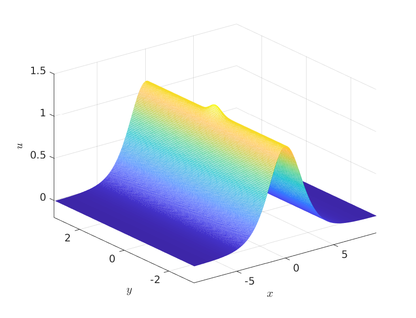
First we consider localized perturbations of the line soliton of the form (17) with a speed ; we choose so that , and in such a way that the perturbation is localized on the computational domain.
The initial data can be seen on the left of Fig. 1. For the time evolution we use time steps for . It can be seen on the right of Fig. 1 that some radiation is emitted but that the norm of the solution stabilises on some plateau.

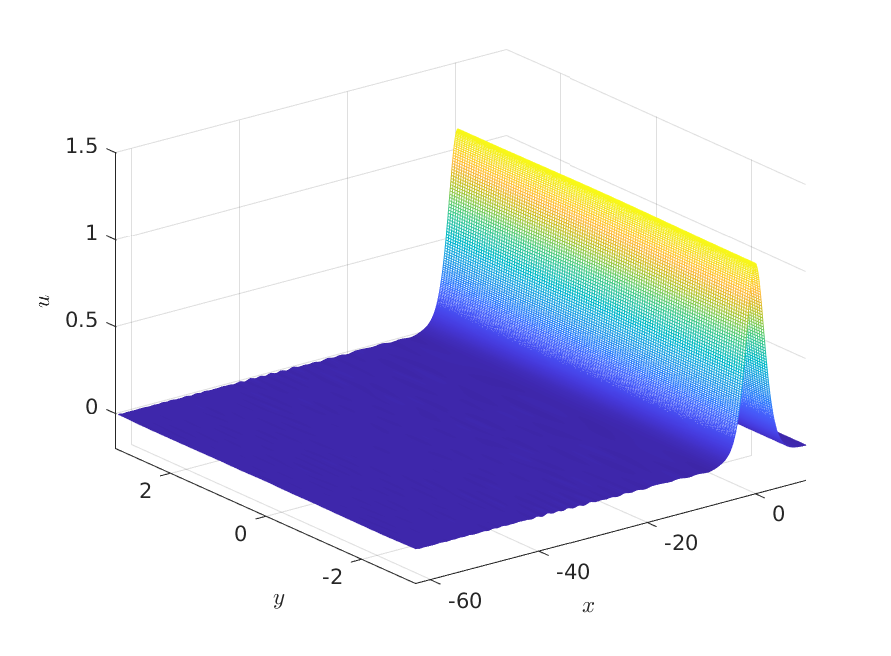
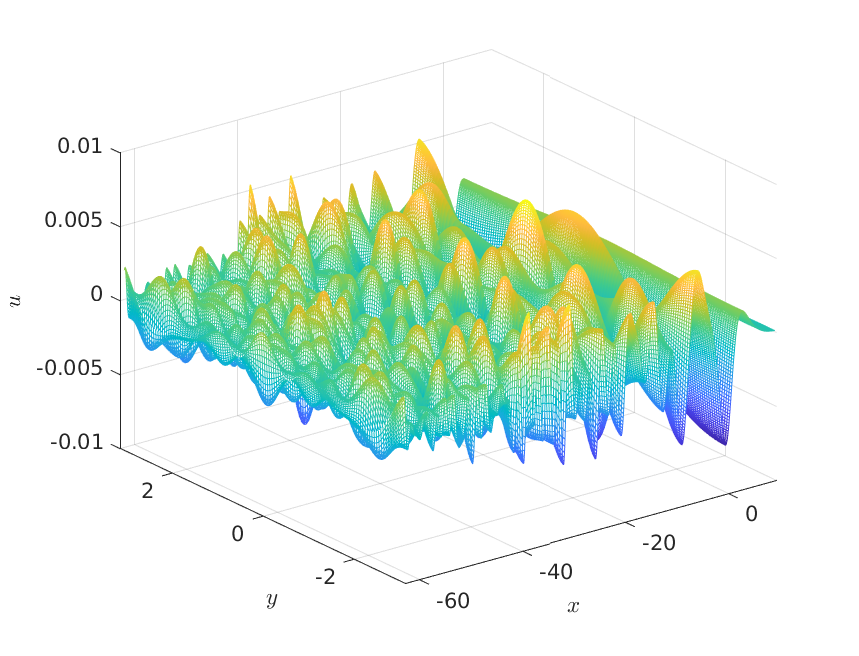
The behavior of the norm indicates that the final state is a line soliton with slightly different mass (in order to see numerically in finite time effects of the perturbation, we had to consider a perturbation with a mass of a few percent of the unperturbed soliton; thus though the soliton is clearly stable, the mass of the final state is slightly different from the one of the unperturbed soliton). On the left of Fig. 2 we show the solution for . To compare this final state to (2), we simply determine the speed of the soliton (2) having the same maximum as the final state. On the right of Fig. 2 one can see that the difference of the final state and a line soliton with a fitted value of the speed is within of the maximum of the initial data, the same order of magnitude as the radiation. The fitted soliton has speed ratio .
As a second example we consider non-localised, but periodic perturbations in of the form (18) with and , , following the same reasoning as before. The initial data can be seen on the left of Fig. 3. The time dependence of the norm on the right of the same figure once more indicates that the solution is stable, and that the final state is a line soliton of slightly different mass.
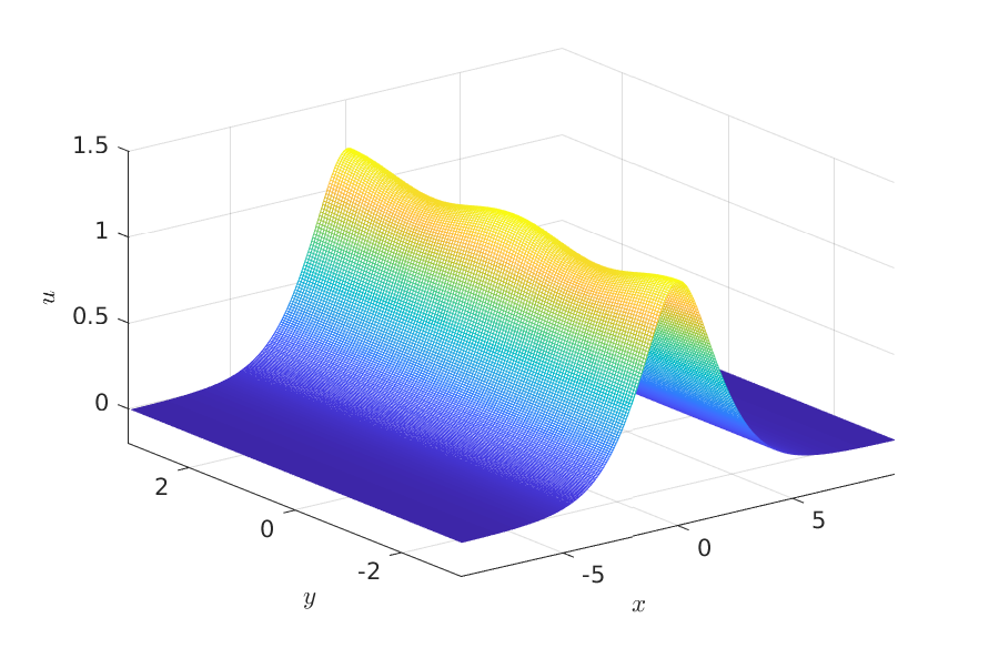
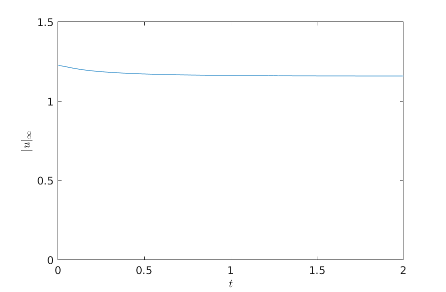
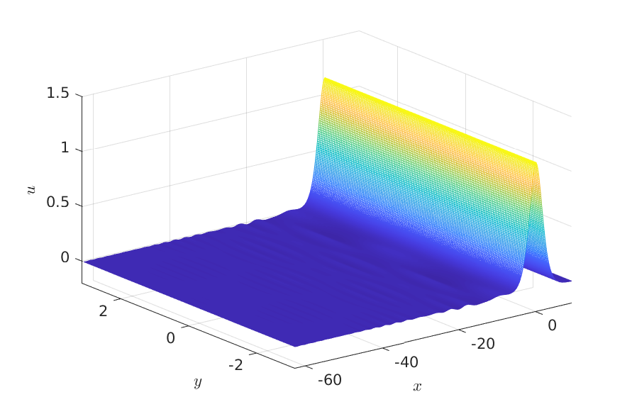
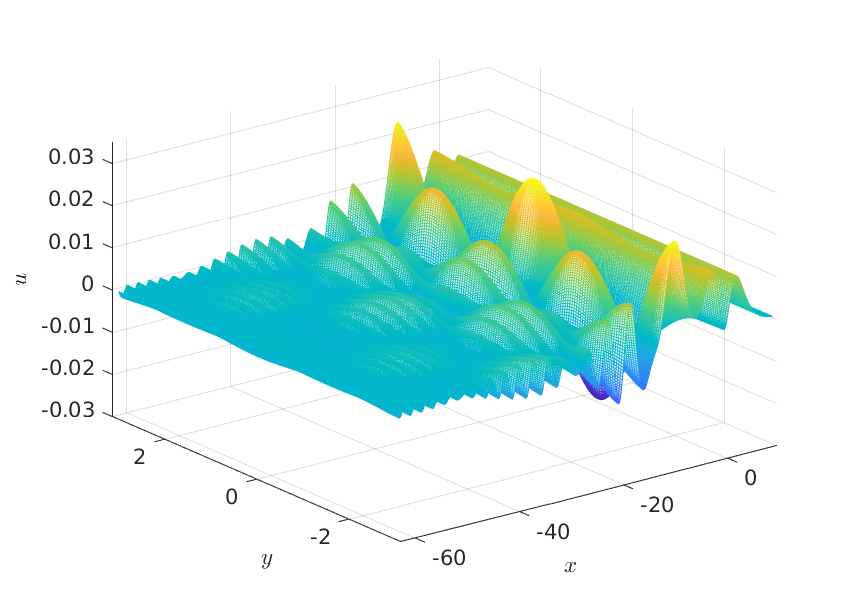
The final state of the solution is shown on the left of Fig. 4. It is within of the fitted line soliton (2) as can be seen on the right of the same figure. The fitted soliton has speed ratio .
3.2. Unstable regime
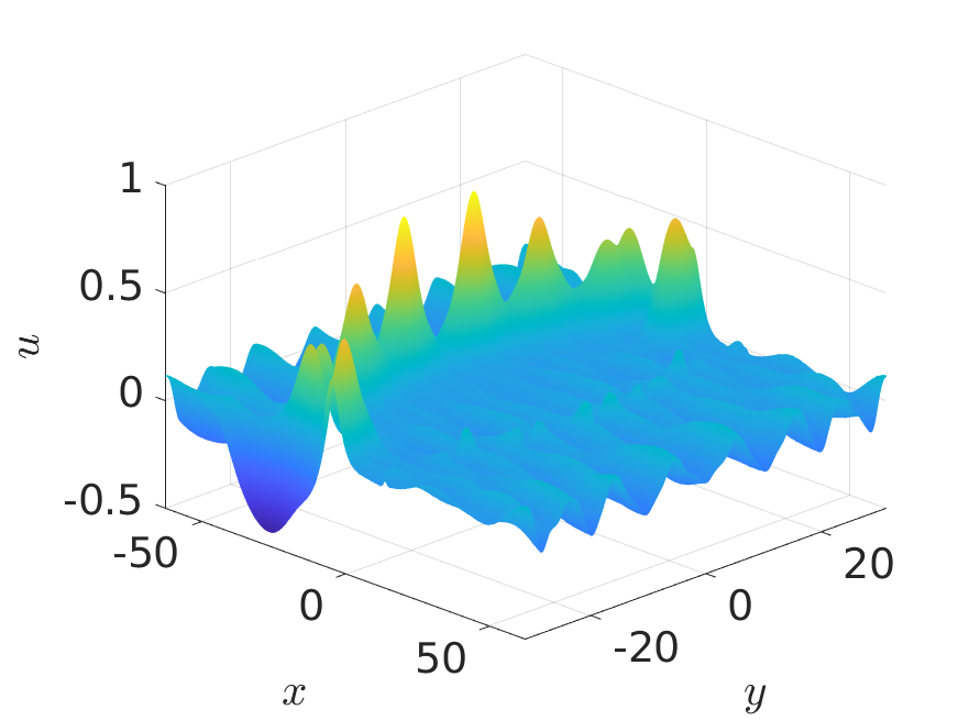
In this subsection we consider the unstable regime. To do this we study similar initial conditions as in the stable case. However, we change the domain and consider with Fourier modes. We first study the localized perturbation (17) with and and soliton speed for using time steps. The initial data are similar to the ones on the left of Fig. 1. As (we use in order to see lump formation on the chosen computational domain before radiation re-entering the domain having an effect on the results), the instability is clearly visible in the norm of the solution on the left of Fig. 6.


The initial data appear to decompose into an array of lumps as in the KP case, see [23], as can be recognized in Fig. 5. To show that the array of peaks can indeed be interpreted as an array of lumps, we fit the solution to a multi-lump solution. As the lumps are exponentially localised, such a solution can be constructed as a sum of single soliton solutions, provided the peaks are sufficiently far away from each other, which is the case here (we simply subtract the solution of (5) after applying the scaling (6) at the maximum). The difference between the solution and the fitted multi-soliton is shown in Fig. 6 on the right. Locally, the difference is again of the order of magnitude of the radiation, however we can see a possible development of a second wave of smaller solitons at the back. Mass re-entering the domain in the direction does not allow us to investigate this development further.

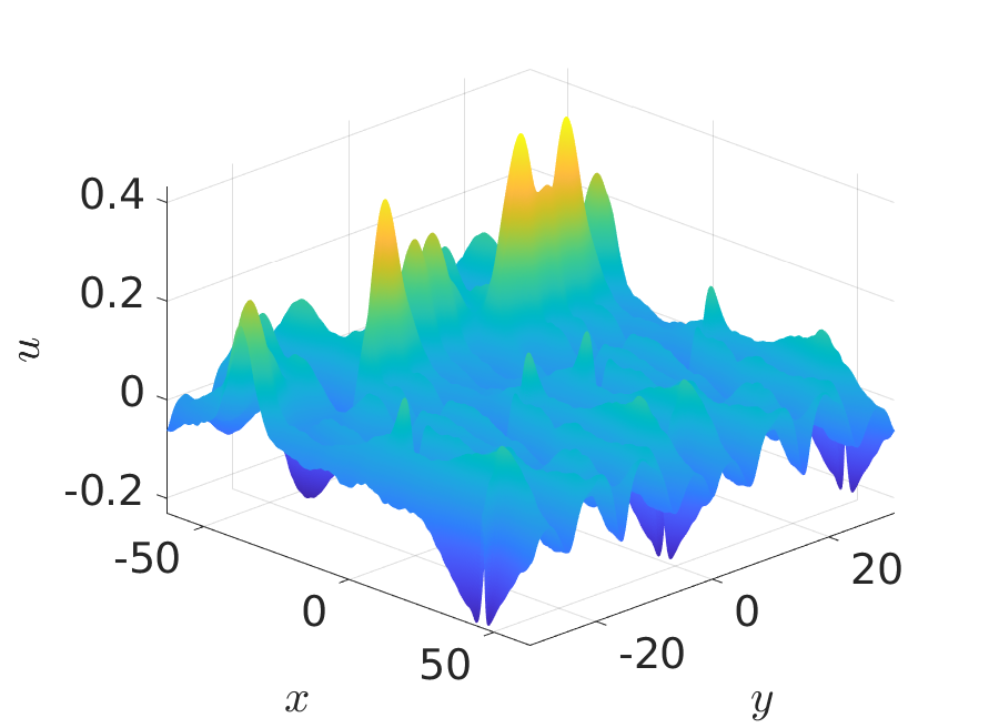
Next, we study periodically perturbed initial data of the form (18) with , , , and the same numerical parameters as in the previous case, see the left of Fig. 3. The norm on the left of Fig. 8 indicates the instability of the line soliton.


The solution for for these initial data is shown in Fig. 7. Once more an array of lumps appears to form. By fitting the peaks to a lump, we can identify eight lump solitons, with a fit correct to 2%, i.e., of the error of the radiation, as can be seen in the right of Fig. 8.

4. Critical nonlinearity
In this section we address the critical case. Three variables determine the stability of the line soliton, as in the theorem in [46]: the size of the cylinder (in our case this is a torus, however the longitudal dimension is sufficiently large to treat it as a cylinder), the speed of the line soliton and the size of the deformation. We are not aware of analytical results in this direction. We consider cases where a small perturbation, that is, a perturbation with a norm within 10% of the infinity norm of the line soliton. We expect two regimes as before though the critical speed , below which the line soliton is stable, is not known in this case. Numerically it is difficult to determine the critical speed, however we show that a sufficiently small and slow line soliton is stable. For larger values of , lump formation is possible, however since the lumps are conjectured to be unstable against blow-up, see [21], an blow-up as in Conjecture 1 of [21] can be also observed here. We do not go into details here since the results appear to be in accordance with what has been found in [21].
If the speed of the line soliton is smaller than some unknown critical value , we expect the line soliton to be stable under small perturbations. This is indeed shown by a numerical experiment on the left of Fig. 9. We see for the norm that a small line soliton with stabilises under a small local Gaussian perturbation of the form (17). Since the latter is finite in order to see numerical effects for finite computing times, the solution tends to a line soliton with slightly different speed. The difference in height between the unperturbed initial soliton and the final one is about 2%.


In contrast, if the speed we expect the line soliton to be unstable against lump formation that are in turn unstable against a blow-up. As the numerical code cannot come arbitrarily close to a singularity without losing precision, we can track the solution only until close to the time of formation of a first singularity. Whether or not the solution forms additional singularities at the location of other lumps at a later time cannot be answered with the present means. We will only address below the question of the first singularity to appear. We are able to recover the blow-up rate by using a multi parameter fit on the evolution of according to (7) to the expression,
| (19) |
where we fit for the critical time , blow-up rate and parameter using least squares. We use data points that are sufficiently close to the blow-up, but for which the conservation of mass is still sufficient. The fitting parameters given in the caption of Fig. 10 do not depend significantly on the number of points used for the fitting. In our plots on Fig. 10 and 12 on the right we include points that are not used for the fitting, in order to better illustrate the three regimes: non-critical regime on the right of the figure, when the solution is far away from the blow-up point, followed by a section that is sufficiently close to the blow-up, and the solution is well tracked and the red line and the blue curve match, and finally on the left of the plot the numerical scheme loses the solution.
Remark 4.1.


The code is stopped once the numerically computed mass is no longer conserved relatively to better than . The solution for is shown on the left of Fig. 11. On the right of the same figure, we show the difference between the peak and a dynamically rescaled lump. It can be seen that the lump gives the blow-up profile to the order of 2% though the singularity is not yet reached. Note that the singularity is formed at the same position as the initial (positive) deformation. A negative deformation of sufficient mass produces a blow-up in the opposite - direction.

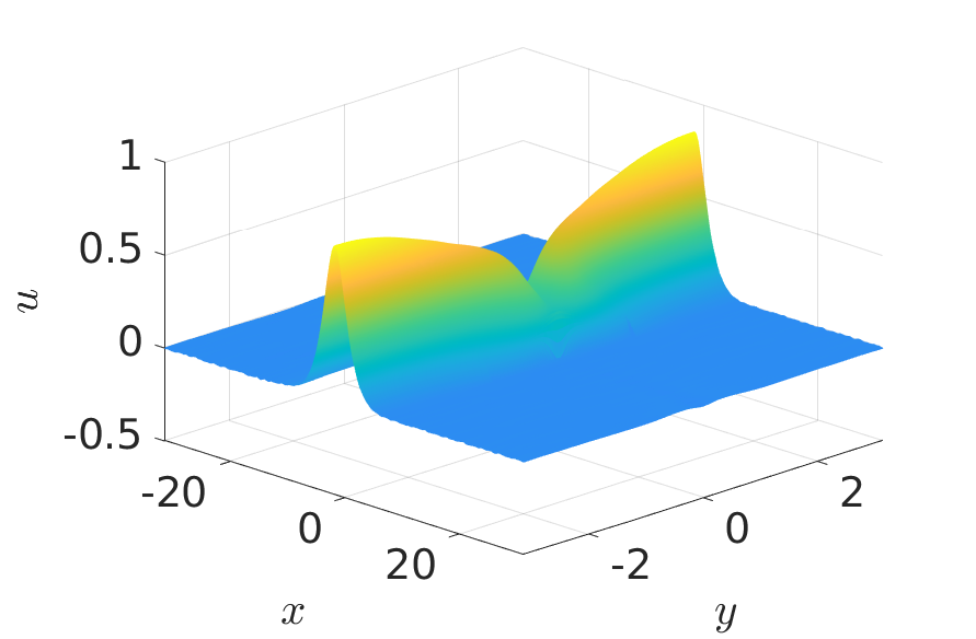
We now look at a periodic perturbation on a large torus with period in -direction. Here we take , so that the expected two lumps are not in a strong interaction regime, see [21] for fusion of ZK lump solutions, and initial condition (18)
where , , and . The evolution of the norm of the solution for these initial data as well as the blow-up rate are shown on Fig. 12. We note that the solution blows up simultaneously at two spatial points and that the coordinates of these two points are where the initial deformation is minimal.


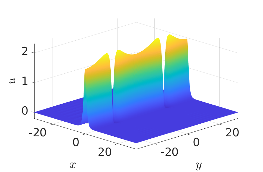
The code is stopped once a lack in mass conservation indicates a loss of accuracy. We show on the left of Fig. 13 the solution at this time, . On the right of the same figure we show the difference between this solution and lumps fitted to the peaks.

5. Super-critical nonlinearity
In the super-critical case we expect a similar behaviour as in the critical case, namely two regimes depending on the speed of the initial line soliton. If , where is once more unknown, the final state is a line soliton of slighly different mass. This is indeed shown by a numerical experiment described in Fig. 9 on the right, that tracks the norm for the initial data (17) with and with . We see that a small line soliton perturbed by a small Gaussian leads to a final state being a line soliton of slightly different speed. The difference in height between the unperturbed initial condition and the final is about 2%. We observe the same behaviour for different types of deformations e.g. localised in and periodic in or localised negative deformations.
For supercritical speeds, the behaviour is similar to the critical case, and again we observe simultaneous blow-up at two different spatial points in the periodically deformed case for periodically perturbed initial data (18), see Fig. 14 on the right. The behavior for a Gaussian perturbation (17) is shown on the left of the same figure. The observed blow-up rates are close to as predicted by the self-similar mechanism conjectured in [21].


We show the solutions close to blow-up in Fig. 15, on the left for a localized perturbation, on the right for a deformed line soliton. It can be seen that lump-like structures form in both cases which will eventually blow up.


6. Conclusion
In this paper we have presented a detailed numerical study of perturbations of line solitons on approximating a situation on . We consider perturbations being localised both in and and perturbations localised in , but periodic in , i.e., deformed line solitons. It was shown that the line soliton is stable for smaller than some critical speed , also in critical and supercritical cases (but subcritical in 1D). In the latter cases, the precise value of appears to be unknown. For values of , the line soliton appears to be unstable against lump formation. Since the lumps are known to be strongly unstable in the critical and supercritical cases, a blow-up in finite time was observed in these settings.
An interesting question would be to determine the value of the critical speed which is numerically difficult, but could be accessible analytically. Since the ZK equation can also be studied in 3D, the 2D lumps can be extended to line solitons of the 3D ZK equation. The transverse stability of these solutions will be studied numerically in an ensuing work.
References
- [1] J. Arbunich, C. Klein, C. Sparber, On a class of derivative Nonlinear Schrödinger-type equations in two spatial dimensions, M2AN 53(5), (2019), 1477 - 1505.
- [2] H. Berestycki and P.-L. Lions, Nonlinear scalar field equations, Arch. Rational Mech. Anal. 82 (1983), 313-376.
- [3] R. Côte, C. Muñoz, D. Pilod, and G. Simpson, Asymptotic stability of high-dimensional Zakharov-Kuznetsov solitons, Arch. Ration. Mech. Anal. 220 (2016), no. 2, 639–710.
- [4] S. Cox and P. Matthews, Exponential Time Differencing for stiff Systems, J. of Comp. Phys., 176 (2002), 430-455.
- [5] A. de Bouard, Stability and instability of some nonlinear dispersive solitary waves in higher dimension, Proc. Roy. Soc. Edinburgh Sect. A 126 (1996), no. 1, pp. 89–112.
- [6] T.J. Bridges, Universal geometric conditions for the transverse instability of solitary waves, Phys. Rev. Lett. 84 (2000), 2614-2617.
- [7] A. V. Faminskii, The Cauchy problem for the Zakharov-Kuznetsov equation. (Russian) Differentsialnye Uravneniya 31 (1995), no. 6, 1070–1081, 1103; translation in Differential Equations 31 (1995), no. 6, 1002–1012.
- [8] L.G. Farah, F. Linares and A. Pastor, A note on the 2D generalized Zakharov-Kuznetsov equation: Local, global, and scattering results, J. Diff. Eq. 253 (2012), 2558–2571.
- [9] L. G. Farah, J. Holmer and S. Roudenko, Instability of solitons - revisited, II: the supercritical Zakharov-Kuznetsov equation, Contemp. Math., 725, Amer. Math. Soc., 89–109.
- [10] L. G. Farah, J. Holmer and S. Roudenko, Instability of solitons in the 2d cubic Zakharov-Kuznetsov equation, Fields Institute Communications, vol 83 (2019), Eds: Miller P., Perry P., Saut JC., Sulem C., Nonlinear Dispersive Partial Differential Equations and Inverse Scattering. Springer, New York, NY
- [11] L. G. Farah, J. Holmer, S. Roudenko and Kai Yang, Blow-up in finite or infinite time of the 2D cubic Zakharov-Kuznetsov equation, arXiv:1810.05121
- [12] D. Han-Kwan, From Vlasov-Poisson to Korteweg and Zakharov-Rubenchik, Comm. Math. Phys. 324, no.3 (2013), 961-993.
- [13] M. Hochbruck, A. Ostermann, Exponential integrators, Acta Numerica (2010), pp. 209-286, doi:10.1017/S0962492910000048
- [14] H. Iwasaki, S. Toh and T. Kawahara, Cylindrical quasi-solitons of the Zakharov-Kuznetsov equation, Physica D 43 (1990), 293-303.
- [15] A. Kazeykina and C. Klein, Numerical study of blow-up and stability of line solitons for the Novikov-Veselov equation, Nonlinearity 30, 2566-2591 (2017)
- [16] S. Kinoshita, Global well-posedness for the Cauchy problem of the Zakharov-Kuznetsov equation in 2D, Ann.I.H. Poincaré-AN 38 (2021), 451-505.
- [17] C. Klein, Fourth order time-stepping for low dispersion Korteweg-de Vries and nonlinear Schrödinger equation, ETNA Vol. 29 116-135 (2008).
- [18] C. Klein and R. Peter, Numerical study of blow-up in solutions to generalized Kadomtsev-Petviashvili equations, Discrete Contin. Dyn. Syst. Ser. B 19 (2014), 1689-1717.
- [19] C. Klein and R. Peter, Numerical study of blow-up in solutions to generalized Korteweg-de Vries equations, Phys. D 304 (2015), 52-78.
- [20] C. Klein and K. Roidot, Fourth order time-stepping for Kadomtsev-Petviashvili and Davey-Stewartson equations, SIAM J. Sci. Comput., 33(6), 3333-3356. DOI: 10.1137/100816663 (2011).
- [21] C. Klein, S. Roudenko, N. Stoilov, Numerical study of Zakharov-Kuznetsov equations in two dimensions, J. Nonl. Sci 31(26) (2021) https://doi.org/10.1007/s00332-021-09680-x
- [22] C. Klein, S. Roudenko, N. Stoilov, Numerical study of soliton stability, resolution and interactions in the 3D Zakharov-Kuznetsov equation, Physica D 423 (2021) 132913, https://doi.org/10.1016/j.physd.2021.132913
- [23] C. Klein and J.-C. Saut, Numerical study of blow up and stability of solutions of generalized Kadomtsev-Petviashvili equations, J. Nonl. Sci. Vol. 22 (5), 763-811 (2012).
- [24] C. Klein and N. Stoilov, A numerical study of blow-up mechanisms for Davey-Stewartson II systems, Stud. Appl. Math., DOI : 10.1111/sapm.12214 (2018)
- [25] E.A. Kuznetsov, Stability criterion for solitons of the Zakharov–Kuznetsov-type equations, Physics Letters A 382 (2018) 2049–2051
- [26] E.A. Kuznetsov, A.M. Rubenchik, V.E. Zakharov, Soliton Stability in plasmas and hydrodynamics, Phys. Rep. 142(3) (1986) 103-165.
- [27] M.K. Kwong, Uniqueness of positiv eradial solutions of in , Arch. Rational Mech. Anal. 105 (1989), 243-266.
- [28] Yang Lan, Stable Self-Similar Blow-Up Dynamics for Slightly -Supercritical Generalized KDV Equations, Communications in Mathematical Physics volume 345, pages 223–269 (2016)
- [29] D. Lannes, F. Linares and J.-C. Saut, The Cauchy problem for the Euler-Poisson system and derivation of the Zakharov-Kuznetsov equation, Prog. Nonlinear Diff. Eq. Appl., 84 (2013), 181–213.
- [30] F. Linares and A. Pastor, Well-posedness for the two-dimensional modified Zakharov-Kuznetsov equation, SIAM J. Math. Anal. 41, no. 4 (2009), 1323–1339.
- [31] F.Linares, A. Pastor and J.-C. Saut, Well-posedness for the ZK equation in a cylinder and on the background of a KdV soliton, Comm. Partial Diff. Eq. 35 9 (2010), 1674-1689.
- [32] Y. Martel and F. Merle, Blow up in finite time and dynamics of blow up solutions for the -critical generalized KdV equation, J. Amer. Math. Soc. 15 (2002), 617–664.
- [33] S. Melkonian and S. A. Maslowe, Two dimensional amplitude evolution equations for nonlinear dispersive waves on thin films, Phys. D 34 (1989), pp. 255–269.
- [34] F. Merle, Existence of blow-up solutions in the energy space for the critical generalized KdV equation, J. Amer. Math. Soc. 14, no. 3, (2001), 555–578.
- [35] L.Molinet and D. Pilod, Bilinear Strichartz estimates for the Zakharov-Kuznetsov equation and applications, Ann.I. H. Poincaré-AN 32 (2015), 347-371.
- [36] S. Munro and E. J. Parkes, The derivation of a modified Zakharov-Kuznetsov equation and the stability of its solutions, J. Plasma Phys. 62 (3) (1999), 305–317.
- [37] D. Pelinovsky Normal form for transverse instability of the line soliton with a nearly critical speed of propagation Math.Model.Nat. Phenom. 13 (2018), 1-20.
- [38] X. Pu, Dispersive limit of the Euler-Poisson system in higher dimensions, SIAM J. Math. Anal. 45 no. 2 (2013), 834-878.
- [39] F. Ribaud and S. Vento, A note on the Cauchy problem for the 2D generalized Zakharov-Kuznetsov equations, C. R. Math. Acad. Sci. Paris 350 (2012), no. 9-10, 499–503.
- [40] F. Rousset and N. Tzvetkov, Stability and instability of the KdV solitary wave under the KP-I flow, Comm. Math. Phys., 313 (2012), no. 1, 155–173.
- [41] F. Rousset and N. Tzvetkov, Transverse nonlinear instability of solitary waves for some Hamiltonian PDE’s, J. Math.Pures Appl. 90 (2008), 550-590.
- [42] Y. Saad and M. Schultz, GMRES: a generalized minimal residual algorithm for solving nonsymmetric linear systems, SIAM J. Sci. Comput. 7 (1986), 856-869.
- [43] R. Sipcic, D. J. Benney, Lump Interactions and Collapse in the Modified Zakharov-Kuznetsov equation, Stud. Appl. Math. 105 (4) (2000), 385–403.
- [44] C. Sulem, P.-L. Sulem, The nonlinear Schrödinger equation. Self-focusing and wave-collapse. Springer, 1999.
- [45] F. Valet, Asymptotic K-soliton-like solutions of the Zakharov-Kuznetsov type equations, Transactions AMS 374 (5) (2021), 3177-3213.
- [46] Y. Yamazaki, Stability for line solitary waves of Zakharov-Kuznetsov equation, Journal of Differential Equations, Volume 262, Issue 8, (2017), 4336-4389.
- [47] Y. Yamazaki, Center stable manifolds around line solitary waves of the Zakharov-Kuznetsov equation with critical speed, arXiv : 2004.10088v1 20 Apr 2020.
- [48] K. Yang, S. Roudenko and Y. Zhao, Blow-up dynamics in the mass super-critical NLS equations, Phys. D, 396:47–69, 2019.
- [49] V.E. Zakharov and E.A. Kuznetsov, On three dimensional solitons, Zhurnal Eksp. Teoret. Fiz, 66 (1974), 594–597 [in russian]; Sov. Phys JETP, vol. 39, no. 2 (1974), pp. 285–286.
- [50] http://www.mathphys.fr