A Framework for Reconstructing COVID-19 Transmission Network to Inform Betweenness Centrality-Based Control Measures
Abstract
In this paper, we propose a general framework for optimal control measures, which follows the evolution of COVID-19 infection counts collected by Surveillance Units on a country level. We employ an autoregressive model that allows to decompose the mean number of infections into three components that describe: intra-locality infections, inter-locality infections, and infections from other sources such as travelers arriving to a country from abroad. We identify the inter-locality term as a time-evolving network and when it drives the dynamics of the disease we focus on its properties. Tools from network analysis are then employed to get insight into its topology. Building on this, and particularly on the centrality of the nodes of the identified network, a strategy for intervention and disease control is devised.
Keywords:
Optimal control,keywords
Research
1 Introduction
Many studies have appeared in the literature to address a wealth of questions about the COVID-19 pandemic, covering a range of disciplines from medicine, genetics, pharmacology to social and economic sciences [1, 2]. Some of these studies have a regional focus, investigating the disease in countries, or regions of a country, while others have considered the pandemic in larger geographical contexts [3, 4, 5].
Modeling the evolution of the disease has been one of the main quantitative approaches used, especially with the goal of forecasting numbers of affected cases. It has also been at the heart of subsequent investigations on practical aspects: from management of resources (assessment of the preparedness for disease containment and readiness of the healthcare system) to possible intervention measures (vaccination and testing strategies [6], government control measures) and their consequences [7]. The different types of modeling that have been applied to investigate the dynamics of COVID-19 infections have a long history in epidemic modeling. Compartmental models (e.g., SIR, SIER) are a well known class of models. They study the interplay between susceptible, infected and recovered individuals within communities, with different degrees of spatial refinement. For instance, in the so called networked compartmental models, interactions between communities are encoded in a network [8], often to identify the spatial and temporal origin of the disease [9]. In statistics, spatial/and/or temporal point processes are often employed to study the dynamics of the disease. Some models allow for the number of infections to be triggered by those at previous times, others can incorporate, as covariates, additional available information such as demographics, human mobility, and policy decisions. Some recent work on COVID-19 follows this direction [10, 11, 12]. Epidemic models can also be recast in a standard regression framework, where the time series of infection counts are fitted by specifying a distribution for the counts and the associated conditional mean function [13, 14]. In most of these studies, the goal is to predict and capture the spatio-temporal patterns of disease spread. Recently, this approach was implemented on COVID-19 data [3, 4, 5]. In this paper, we propose a framework for optimal control measures. The first component of the framework hinges on a statistical regression analysis of infection counts over time and aggregated over localities in a country, with a mean function that takes account of the spatial proximity of these localities. The fitted model is then used to reconstruct a weighted network, which constitutes the second component of our framework. The salient point of our method of network recovery is that smoothness conditions on the temporal data are not required [15], and neither is the near steady-state dynamics that is instead necessary for the perturbation/response approaches to work [16, 17, 18]. Our reconstruction is similar to that in [19], while it differs from procedures that rely on the deterministic evolution of the disease [20, 21]. The third component of our framework is the study of the changes in the topology of the underlying recovered network and the computation of centrality measures (specifically the nodes’ betweenness centrality), from which the recommendation of optimal control measures ensues. We apply the method in the case of Lebanon.
2 Model Definition
Our starting point of the analysis is a statistical model that captures the spatio-temporal dynamics of the infections, under the statistical framework discussed in [13]. Namely, we consider the number of infections recorded in a given locality in a given day , as independent, conditionally on the counts at previous times, random variables distributed according to a negative binomial distribution having a mean function decomposed into three terms as follows:
| (1) |
The first two terms constitute the auto-regressive part of the model: one being the contribution to the mean infection in locality at time , due to the infections within at the previous day, the other being the contribution to due to positive cases from other localities also at the previous day. The final term accounts for all other contributions not captured by the first two, such as infected people who entered the country under study from abroad. For simplicity we will refer to the last term as the component due to travel and assume that it is proportional to the size of the population of the locality. The log-transforms of non-negative coefficients and , which quantify the contribution of the past observations to future counts, and the log-transform of the parameter are each modeled as a linear function of time, with a locality-specific slope to allow more flexibility across localities. Intercepts and slopes are estimated from the data. Finally, we model as a power function of the geographical distance of the localities: . This is assumed because previous studies have shown that mobility flows are governed by power-law functions of inter-localities distances [22, 23, 24, 25].
3 Data Description and Fitting of the Regression Model
As an application of the framework, the model (1) was applied to the COVID-19 data collected in Lebanon. On daily basis, the laboratories from the public and private sectors report the confirmed cases to the Epidemiological Surveillance Program of Lebanon’s Ministry of Public Health (ESUMOH). Later, the cases are investigated in order to get additional demographic information and health condition. The data are then archived in a national platform. Specifically, the data we have considered consist of counts of COVID-19 recorded daily in each of the 1544 localities of Lebanon from February 21, 2020 to January 20, 2022. Such localities correspond to Lebanon’s smallest statistical units called “circonscriptions foncières” or cadastral villages following the Central Administration for Statistics (CAS) nomenclature [26]. Recommendations on possible interventions and updates on the disease evolution were sought for by the Ministry of Public Health at 20 days intervals. Model (1) was fitted using the R package surveillance [14] over the intervals , for . This allows us to follow the evolution in time of the model parameters until day 700, the last observation point.
Figure 1 displays the aggregated counts over all localities, , and the fitted values over the complete time period of our study broken down into the three components of the mean function. The fit appears quite adequate. It is in fact a better fit to the data than the model with counts assumed to be Poisson-distributed, which is an indication of overdispersion in the data. A further comparison of these two models in terms of AIC value and prediction errors is provided in Table 1.
| ses | AIC | |
|---|---|---|
| Negative Binomial | 2.88 | 1164119 |
| Poisson | 3.65 | 1333453 |
We further notice that the model of equation (1) considers a time-lag of one day; that is, the future counts depend on the counts recorded on the previous day. Changes in the time-lag from one to a few days did not result in any noticeable difference. Our analysis provides evidence that the inter-locality infection drives the overall transmission of the disease [22]. Then, for this reason we shift our focus to the network that governs the interaction between localities and observe that it is not purely a static spatially-dependent network but rather dynamic and time-evolving: in fact the product of time-dependent coefficients with the spatial proximity matrix. Figure 1 indicates that the inter-locality term has the most important contribution to the increase in the mean number of infections compared to the intra-locality and travel terms. This suggests that the inter-locality transmissions should be the main focus of analysis, and what one learns from their study would be useful for disease control.
The parameter estimates of model (1) for all 1554 localities and their errors can not be displayed in an uncluttered fashion but are available from the corresponding authors. A sample of the evolution of the inter-locality term is shown in Figure 2.
4 Network Identification and Characterization
As has emerged from the statistical model, the inter-locality dynamics plays the major role in determining the infection numbers. While this may seem to contradict previous studies, for example [27], on the secondary attack rate being mostly driven by household interactions, it is worth noting that infections outside households are hard to pin down, and thus this may be a limitation in such studies. We wish to focus now on the inter-locality term and study it from a different perspective. To do so, observe that the second term in the mean equation (1) can be re-written as follows: , where . It can be interpreted as the contribution to the cases at time in locality from cases from locality at the previous day. We can suggestively think of as defining the weights of a network between localities: the transport network describes the traffic flow between localities, and thus predates the disease, while is the number of transported cases from into neighboring localities. explicitly depends on since the coefficients of , which are linear functions of , and the power in the definition of are estimated over each interval . An example is provided in Figure 3 which is a graphical representation of . The superscript in the notation of indicates that the latter was estimated on the counts data of contiguous 20-day time intervals, that is the 300-day time span from February 21, 2020 to December 16th, 2020. This complex network drives the cross-localities dynamics. We will now suggest employing some useful summary metrics for and its time evolution in order to understand its properties, and accordingly prescribe adequate control measures.

One useful summary metric is the modularity, which is a measure of cluster formation in a network. More specifically, the modularity of a given network is defined with respect to a given grouping of its nodes. We follow [28] where the grouping of the nodes is determined by a stochastic procedure that reveals densely connected subgraphs. An illustration of a grouping is given in Figure 4.
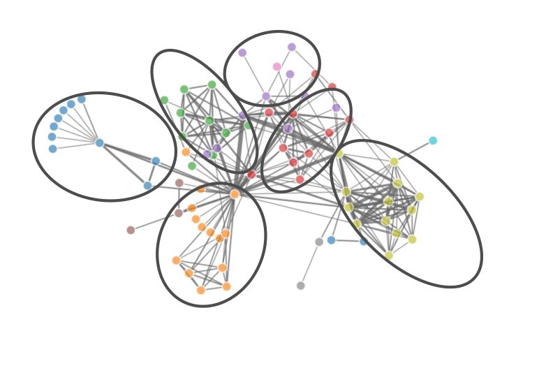
Given this group membership, the modularity of is then computed according to the formula:
where denotes the total number of edges, and are the degree of nodes and respectively, labels the group to which belongs, and is the Kronecker delta. Figure 5 shows the modularities of the 35 matrices at days for . The superscript in the notation , as mentioned above, indicates that is estimated using the counts of the days of the study. One can see a jump in modularity on the tenth 20-day time interval, which we will denote by . This behavior may signal the onset of an emerging power-law [29]. We investigate if this is the case by analyzing two additional topological measures for the networks: mainly, the clustering coefficient and the average path length [30, 31]. These are generally used to classify networks into random, scale-free, or regular.
The clustering coefficient of a network is a measure of transitivity that counts the ratio of the number closed triplets to the number of all (closed and open) triplets. A triplet is closed if all the three connections between the three nodes exist and is open if one of the links is missing. The average path length of a network is given by the mean distance over all pairs of vertices, where distance is the number of edges in the shortest path joining them. An illustration is shown in Figure 6.
Small-world or scale-free networks (that is, networks with node degrees and strengths distributed according to a power-law) are characterized by high clustering coefficients and low average path lengths compared with those of regular/ordered graphs [31, 30]. Random graphs are, on the other hand, characterized by low average path lengths and low clustering coefficients compared to regular graphs. An illustration of the three different network types is shown in Figure 7.
Figure 8 shows the clustering coefficients and the average paths lengths for the matrices . Similar behavior of both and was observed for all , with .
The evolution of both and gives additional evidence for a transition at a point . The clustering coefficient starts suddenly to increase. At the -th interval there is an abrupt jump in the average path length as well at (Figure 8). This is an indication of scale-freeness of the network. This property expedites the spread of epidemics unlike what would occur in ordered networks, which are characterized by a slower spread because they possess a high and an that scales with system size [32, 33].
To characterize the transition to scale-freeness, we now analyse the distribution of the strengths of the nodes, as additional evidence for change in the network topology at the -th interval . A node’s strength is the sum of the weights of its edges. Namely, for the -th node:
Figures 9 and 10 show the empirical and estimated distributions of the strengths (in fact, the survival function ) of , at the time intervals on a log-log scale. We note that a transition occurs at , where the distribution becomes linear, which is indicative of a power-law (Pareto distribution): , for . The exponent and the boundary value (scale) are estimated by maximum likelihood following [34].


Figure 11 summarizes the estimates of the exponents for these networks and their standard errors (obtained by non-parametric bootstrap).
After the 180th day, that is for time intervals labeled by the index , most power-laws have very close exponents of about 2.5. This signals the stabilization of the network topology. Thus, marks the onset of the emergence of the steady state network. We think that only above this point any prescription of control measures is likely to be efficient as the revealed network topology, relying on the daily counts, has stabilized. One can wonder if there is any explanation on why the stable phase has set in during this interval , and not before or after it. chronologically coincides with the period between August, 19, 2020, and September 7, 2020. Perhaps, the blast in Beirut which occurred on August 4th and in the following weeks of social protests, personal precaution measures (such as social distancing and wearing of masks) were compromised. Either of these occurrences may have contributed to the detected change in the network type. See the Appendix for the chronology.
5 Putting the analysis into action: Control measures
Having fully characterized the network and identified the steady-state, we now turn to a possible use of this analysis to guide an optimal strategy for disease control. The strategy will identify some localities as candidates for being isolated or for having their connections to other localities curtailed. The measure on which the identification is based is that of centrality of a node. The betweenness centrality of a node is defined as [31]:
where is the total number of shortest paths from node to node passing through . Therefore, the more central the node is, the more its removal has an effect on the network’s connectivity, since its removal would yield a network with more disconnected subgraphs. The control strategy we propose involves an iterative procedure, where at each step the centralities of the nodes are computed, the node with the resulting highest centrality is removed, and the matrix is updated, as illustrated in Figure 12.

Other removal schemes of nodes in network exist, but the one we have just described has been suggested to incur the highest loss of connectivity for scale-free networks [35, 36, 37, 38, 39, 40]. In practice, candidate targets for intervention the localities corresponding to nodes with higher centralities. We notice that at the policy level this strategy based on our analysis was indeed adopted. The localities we have identified through this strategy were given priority in the national vaccination campaign. On the other hand, the recommendations we put forward based on this analysis were only partially adopted in targeting the high centrality localities for lockdown and intervention measures, as the decision making process involved other ministries and stakeholders. However, we conclude by considering theoretically the would-be repercussions of such implementation. Clearly, the loss of connectivity would impede the evolution of the disease since the localities which are contributing the most to the infection would be isolated. For example, removing around of the most connected localities on the basis of their betweenness centrality would lead to loss of connectivity as shown in Figure 13.
Specifically, the localities causing loss of connectivity are shown in Figure 14, while the fitted model of the top sixteen localities is shown in Figure 15. An animated map of the control strategy is available on this hyperlink.


6 Conclusion
In this paper, we have proposed a framework that can be used to inform control measures for epidemics in a country for which infections counts aggregated over local regions are available over time. In particular, we have followed the evolution of the counts of COVID-19 cases in Lebanon at the level of local administrative units at a daily resolution. The framework entails fitting an auto-regressive model to the data; recovering an underlying network over which the disease propagates; analyzing such time-evolving network to identify topological measures of node centrality that suggest an optimal control of the spread of the disease. Specifically, for the data about Covid-19 in Lebanon the analysis of the topological metrics of the network has given us a hint into a transition to a steady state structure that governs interactions between localities. After identifying this steady state network, and characterizing it as a scale-free, we have proposed control measures based on betweenness centrality of its nodes. The findings were taken into consideration in the national vaccination campaign for COVID-19, with the identified localities given priority for vaccination.
Appendix. Chronology of COVID-19 Pandemic in Lebanon
In this appendix we summarize the chronology of the COVID-19 pandemic in Lebanon from the first recorded case to February 2022. We divide this time interval into 4 periods, and highlight the main governmental interventions taken to control the spread of the disease.
Period 1 (February 2020 to June 2020). The first cases are documented. Early lockdown measures are implemented with airport closure. Testing is carried out for suspected cases, close contacts, and travelers. Cases are mainly within clusters. Aggressive contact tracing is adopted.
Period 2 (July 2020 to December 2020): The airport reopens in July 2020. The daily number of cases increases progressively and community transmission sets in. On August 4th, the Beirut blast occurs.
Period 3 (January 2021 to June 2021): The alpha variant is introduced. The case counts increase. Lockdown measures are implemented resulting in a decrease of the recorded cases. However, after lockdown release, an increase of the number of infections is observed until mid-March, with a progressive and sustained decrease up to June.
Period 4 (July 2021 to December 2021). Introduction of the delta variant, which progressively replaces the alpha variant. Two waves of delta are observed: July-September and November-December.
Period 5 (January 2022-February 2022). Introduction of the omicron variant. High transmissibility of the new variant leads to high daily case counts reaching 10,000 on 1st Feb 2022.
References
Acknowledgements
The authors acknowledge the support of Prof. Rima Habib from the AUB’s Faculty of Public Health for her unfailing support and invaluable advice to physicists and mathematicians as they worked with public data as well as Dr. Chadi Abdallah for helping in the early conception of the project.
Funding
The authors received no funding.
Competing interests
The authors declare that they have no competing interests.
Authors’ contributions
J.T contributed to the problem formulation and led the project, and together with S.N and S.M developed the model and numerical analysis involved in this manuscript. G.F and C.A worked on the geographical and the demographic data, R.H and H.S worked on the data processing of infection counts, N.G and H.H on the epidemiological analysis and the significance of the results and their implementation in the vaccination strategy.
References
- [1] Mohamadou, Y., Halidou, A., Kapen, P.T.: A review of mathematical modeling, artificial intelligence and datasets used in the study, prediction and management of COVID-19. Applied Intelligence 50(11), 3913–3925 (2020)
- [2] Guan, J., Wei, Y., Zhao, Y., Chen, F.: Modeling the transmission dynamics of COVID-19 epidemic: a systematic review. Journal of Biomedical Research 34(6), 422 (2020)
- [3] Celani, A., Giudici, P.: Endemic–epidemic models to understand COVID-19 spatio-temporal evolution. Spatial Statistics, 100528 (2021)
- [4] Ssentongo, P., Fronterre, C., Geronimo, A., Greybush, S.J., Mbabazi, P.K., Muvawala, J., Nahalamba, S.B., Omadi, P.O., Opar, B.T., Sinnar, S.A., et al.: Pan-African evolution of within-and between-country COVID-19 dynamics. Proceedings of the National Academy of Sciences 118(28) (2021)
- [5] Dickson, M.M., Espa, G., Giuliani, D., Santi, F., Savadori, L.: Assessing the effect of containment measures on the spatio-temporal dynamic of COVID-19 in Italy. Nonlinear Dynamics 101(3), 1833–1846 (2020)
- [6] Gozzi, N., Bajardi, P., Perra, N.: The importance of non-pharmaceutical interventions during the COVID-19 vaccine rollout. medRxiv (2021)
- [7] Perra, N.: Non-pharmaceutical interventions during the COVID-19 pandemic: A review. Physics Reports (2021)
- [8] Brockmann, D., Helbing, D.: The hidden geometry of complex, network-driven contagion phenomena. science 342(6164), 1337–1342 (2013)
- [9] Schlosser, F., Brockmann, D.: Finding disease outbreak locations from human mobility data. EPJ data science 10(1), 52 (2021)
- [10] Zhu, S., Bukharin, A., Xie, L., Santillana, M., Yang, S., Xie, Y.: High-resolution spatio-temporal model for county-level COVID-19 activity in the US. ACM Transactions on Management Information Systems (TMIS) 12(4), 1–20 (2021)
- [11] Chiang, W.-H., Liu, X., Mohler, G.: Hawkes process modeling of COVID-19 with mobility leading indicators and spatial covariates. International journal of forecasting (2021)
- [12] Giudici, P., Pagnottoni, P., Spelta, A.: Network self-exciting point processes to measure health impacts of COVID-19. Available at SSRN 3892998 (2021)
- [13] Held, L., Höhle, M., Hofmann, M.: A statistical framework for the analysis of multivariate infectious disease surveillance counts. Statistical Modelling 5, 187–199 (2005)
- [14] Meyer, S., Held, L., Höhle, M.: Spatio-temporal analysis of epidemic phenomena using the R package surveillance. arXiv preprint arXiv:1411.0416 (2014)
- [15] Shandilya, S.G., Timme, M.: Inferring network topology from complex dynamics. New Journal of Physics 13(1), 013004 (2011)
- [16] Prabakaran, S., Gunawardena, J., Sontag, E.: Paradoxical results in perturbation-based signaling network reconstruction. Biophysical journal 106(12), 2720–2728 (2014)
- [17] Yu, D.: Estimating the topology of complex dynamical networks by steady state control: Generality and limitation. Automatica 46(12), 2035–2040 (2010)
- [18] Yu, D., Parlitz, U.: Inferring local dynamics and connectivity of spatially extended systems with long-range links based on steady-state stabilization. Physical Review E 82(2), 026108 (2010)
- [19] Wan, X., Liu, J., Cheung, W.K., Tong, T.: Inferring epidemic network topology from surveillance data. PLoS One 9(6), 100661 (2014)
- [20] Pajevic, S., Plenz, D.: Efficient network reconstruction from dynamical cascades identifies small-world topology of neuronal avalanches. PLoS computational biology 5(1), 1000271 (2009)
- [21] Braunstein, A., Ingrosso, A., Muntoni, A.P.: Network reconstruction from infection cascades. Journal of the Royal Society Interface 16(151), 20180844 (2019)
- [22] Meyer, S., Held, L.: Power-law models for infectious disease spread. The Annals of Applied Statistics 8(3), 1612–1639 (2014)
- [23] Zipf, G.K.: The p 1 p 2/d hypothesis: on the intercity movement of persons. American sociological review 11(6), 677–686 (1946)
- [24] Simini, F., González, M.C., Maritan, A., Barabási, A.-L.: A universal model for mobility and migration patterns. Nature 484(7392), 96–100 (2012)
- [25] Barthélemy, M.: Spatial networks. Physics Reports 499(1-3), 1–101 (2011)
- [26] Verdeil, E., Faour, G., Velut, S., Hamzé, M., Mermier, F.: Atlas du LIBAN. Presses de l’Ifpo, ??? (2007)
- [27] Karumanagoundar, K., Raju, M., Ponnaiah, M., Kaur, P., Rubeshkumar, P., Sakthivel, M., Shanmugiah, P., Ganeshkumar, P., Muthusamy, S.K., Sendhilkumar, M., et al.: Secondary attack rate of COVID-19 among contacts and risk factors, tamil nadu, march–may 2020: a retrospective cohort study. BMJ open 11(11), 051491 (2021)
- [28] Fortunato, S.: Community detection in graphs. Physics reports 486(3-5), 75–174 (2010)
- [29] Grindrod, P., Higham, D.J.: High modularity creates scaling laws. Scientific reports 8(1), 1–9 (2018)
- [30] Albert, R., Barabási, A.-L.: Statistical mechanics of complex networks. Reviews of modern physics 74(1), 47 (2002)
- [31] Newman, M.E.: The structure and function of complex networks. SIAM review 45(2), 167–256 (2003)
- [32] Pastor-Satorras, R., Castellano, C., Van Mieghem, P., Vespignani, A.: Epidemic processes in complex networks. Reviews of modern physics 87(3), 925 (2015)
- [33] Newman, M.E.: Spread of epidemic disease on networks. Physical review E 66(1), 016128 (2002)
- [34] Clauset, A., Shalizi, C.R., Newman, M.E.: Power-law distributions in empirical data. SIAM review 51(4), 661–703 (2009)
- [35] Albert, R., Jeong, H., Barabási, A.-L.: Error and attack tolerance of complex networks. nature 406(6794), 378–382 (2000)
- [36] Dong, G., Gao, J., Du, R., Tian, L., Stanley, H.E., Havlin, S.: Robustness of network of networks under targeted attack. Physical Review E 87(5), 052804 (2013)
- [37] Valdez, L.D., Shekhtman, L., La Rocca, C.E., Zhang, X., Buldyrev, S.V., Trunfio, P.A., Braunstein, L.A., Havlin, S.: Cascading failures in complex networks. Journal of Complex Networks 8(2), 013 (2020)
- [38] Buldyrev, S.V., Parshani, R., Paul, G., Stanley, H.E., Havlin, S.: Catastrophic cascade of failures in interdependent networks. Nature 464(7291), 1025–1028 (2010)
- [39] Albert, R., Albert, I., Nakarado, G.L.: Structural vulnerability of the North American power grid. Physical review E 69(2), 025103 (2004)
- [40] Edsberg Møllgaard, P., Lehmann, S., Alessandretti, L.: Understanding components of mobility during the COVID-19 pandemic. Philosophical Transactions of the Royal Society A 380(2214), 20210118 (2021)