Revisiting Multi-breathers in the discrete Klein-Gordon equation: A Spatial Dynamics Approach

Ross Parker Address: Department of Mathematics, Southern Methodist University, Dallas, TX 75275, USA Email address: rhparker@smu.edu , Jesús Cuevas-Maraver Address: Grupo de Física No Lineal, Departamento de Física Aplicada I, Universidad de Sevilla. Escuela Politécnica Superior, C/ Virgen de Africa, 7, 41011-Sevilla, Spain Address: Instituto de Matemáticas de la Universidad de Sevilla (IMUS). Edificio Celestino Mutis. Avda. Reina Mercedes s/n, 41012-Sevilla, Spain Email address: jcuevas@us.es , P. G. Kevrekidis Address: Department of Mathematics and Statistics, University of Massachusetts, Amherst MA 01003, USA Email address: kevrekid@math.umass.edu and Alejandro Aceves Address: Department of Mathematics, Southern Methodist University, Dallas, TX 75275, USA Email address: aaceves@smu.edu

Abstract.

We consider the existence and spectral stability of multi-breather structures in the discrete Klein-Gordon equation, both for soft and hard symmetric potentials. To obtain analytical results, we project the system onto a finite-dimensional Hilbert space consisting of the first $M$ Fourier modes, for arbitrary $M$ . On this approximate system, we then take a spatial dynamics approach and use Lin’s method to construct multi-breathers from a sequence of well-separated copies of the primary, single-site breather. We then locate the eigenmodes in the Floquet spectrum associated with the interaction between the individual breathers of such multi-breather states by reducing the spectral problem to a matrix equation. Expressions for these eigenmodes for the approximate, finite-dimensional system are obtained in terms of the primary breather and its kernel eigenfunctions, and these are found to be in very good agreement with the numerical Floquet spectrum results. This is supplemented with results from numerical timestepping experiments, which are interpreted using the spectral computations.

1. Introduction

Dynamical models on a one-dimensional lattice have been a topic of interest for well over 50 years. Perhaps the most famous example is the Fermi–Pasta–Ulam–Tsingou (FPUT) model [25, 65], which was one of the first problems to be studied using numerical simulations. In this work, we will examine the discrete Klein-Gordon (DKG) equation [14, 21, 20, 43]

(1)

\ddot{u}_{n}=d(\Delta_{2}u)_{n}-f(u_{n}),

which describes the dynamics of an infinitely long, one-dimensional lattice of particles. The quantity $u_{n}$ represents the displacement of the $n$ th particle in the integer lattice as a function of the time $t$ . Each particle is harmonically coupled to its two nearest neighbors via the discrete second difference operator $\Delta_{2}$ , and the strength of this coupling is quantified by the parameter $d$ . The particles are subject to an external, nonlinear, on-site potential $V(u)$ , such that $f(u)=V^{\prime}(u)$ , which can be of different type depending on the model [37, 40]. Common nonlinearities are shown in Table 1. (See Section 2.1 for the definition of hard and soft potentials).

Equation	$V(u)$	$f(u)$
sine-Gordon	$1-\cos u$	$\sin u$
$\phi^{4}$ (soft)	$\frac{1}{2}u^{2}-\frac{1}{4}u^{4}$	$u(1-u^{2})$
$\phi^{4}$ (hard)	$\frac{1}{2}u^{2}+\frac{1}{4}u^{4}$	$u(1+u^{2})$
Morse	$\frac{1}{2}(1-e^{-u})^{2}$	$e^{-u}(1-e^{-u})$

Table 1. Common nonlinearities for the discrete Klein-Gordon equation.

The DKG equation is the discrete analogue of the nonlinear Klein-Gordon partial differential equation

u_{tt}=u_{xx}-f(u),

which is a prototypical model in the study of nonlinear waves and solitons. One of the the most well-studied forms of this equation is the sine-Gordon equation [14, 21, 20, 43], which has periodic nonlinearity $f(u)=\sin(u)$ , and is completely integrable. The transition between the continuous and discrete models in the sine-Gordon case has been extensively discussed in [16]. The discrete sine-Gordon model, also known as the Frenkel-Kontorova model, was originally devised as a model for describing the dynamics of a crystal lattice near a dislocation core [13, 14], and has been used since its inception in numerous additional applications (see, for example, [14]*Chapter 2), including a mechanical model for a chain of pendula [60, 18], arrays of Josephson junctions [61, 29], and DNA dynamics [63, 62, 48].

Two major classes of coherent structures in the nonlinear Klein-Gordon equation (both discrete and continuous) are of particular interest: kinks, which are heteroclinic structures resembling “wave fronts” that connect two adjacent minima of the potential $V(u)$ , and breathers, which are structures that are spatially localized and oscillatory in time. For the continuum sine-Gordon equation, exact, analytical solutions for both of these structures have been found [3]. For discrete systems, the existence and stability of static kinks have been well-studied (see [58, 39, 16], as well as [52] for results on multi-kink solutions), and there has also been interest in moving kinks [6, 33, 17, 4]. We will concern ourselves herein with discrete breather solutions.

Discrete breathers have been studied in Hamiltonian [26] and dissipative systems [28], and have applications in areas such as laser scanning microscopy and coupled optical waveguides [27, 47]. Existence and stability of discrete breather solutions in Klein-Gordon lattices were first studied by MacKay and Aubry [49, 9] by considering the system near the anti-continuum (AC) limit ( $d=0$ ), in which the individual sites in the lattice are uncoupled. The advantage of this approach is that the solution for a single site is known at the AC limit, and this can be continued to small $d>0$ using the implicit function theorem. Some results about asymptotic stability of these breathers can be found in [10]. A similar approach has been used for multi-site solitons in the discrete nonlinear Schrödinger equation (DNLS) [54, 34], which demonstrated that the only potentially stable multi-solitons are those in which adjacent peaks are excited out-of-phase. Analysis of multi-breathers in DKG, in which a finite number of sites in the integer lattice are excited at the AC limit, was done in [7, 45], but this was restricted to the case where the excited sites are adjacent, so that a concrete result could be deduced for the dynamics of the relative phases between oscillators at adjacent sites. Indeed, the two methods (the Aubry band method [9] and the MacKay effective Hamiltonian method [5]) explored in the above two publications were shown to yield the same results near this limit in [19]. In this situation, for small $d>0$ , out-of-phase multi-breathers are stable for soft potentials, and in-phase multi-breathers are stable for hard potentials [7]*Theorem 6. Results on the existence and spectral stability of multi-breathers were extended in [56] to multi-site breathers where any arbitrary, finite set of lattice points is excited at the AC limit; in particular, this allows the excited sites to be separated in the lattice, i.e., there can be “holes” in the lattice. However, spectral stability of multi-breathers does not necessarily imply nonlinear stability; even if the multi-breather is spectrally stable, nonlinear instabilities can result from resonance between internal eigenmodes and the continuous spectrum band, as long as the two have opposite Krein signatures [22] (see also the simpler example of the discrete nonlinear Schrödinger model in [38]). A recent result uses the Schauder fixed point theorem to prove the existence of discrete Klein-Gordon breathers in the setting of a convex on-site potential [32]. Other related work concerns breather solutions in infinite Fermi-Pasta-Ulam-Tsingou (FPUT) lattices, in which the nonlinear potential involves inter-site terms (see [51] and the references therein). Results on the existence of time periodic solutions in FPUT lattices can be found in [51]*Chapter 2, as well as the more recent work in [8, 64].

In this paper, we take a different approach to multi-breathers. We start with a single-site breather, which we call the primary breather. We take the existence of such a breather for a particular $d>0$ as a hypothesis. We then construct a multi-breather by joining together multiple, well-separated copies of this primary breather. Consecutive copies of the primary breather can be either in-phase or out-of-phase. In effect, we replace the condition that the coupling parameter $d>0$ is small with the condition that the individual copies of the primary breather are well separated. The construction of complex coherent structures from simple building blocks has a rich mathematical history (see [59], and the references therein). The mathematical technique that we will use to accomplish this is an implementation of the Lyapunov-Schmidt reduction known as Lin’s method. This method has been successfully employed in many systems, including semilinear parabolic PDEs [59, 24] and discrete dynamical systems [44]. We used a similar method to construct multi-solitons in DNLS [53] and multi-kinks in DKG [52].

Heuristically, we use Lin’s method to construct a double breather from the primary breather as follows (see [53]*Section 1 for a similar construction of double pulses in DNLS). Let $q_{n}(t)$ be the primary breather solution to Eq. 1 with period $T$ , i.e. $q_{n}(t+T)=q_{n}(t)$ for all integers $n$ . Then a $T$ -periodic solution $u_{n}(t)$ is a double breather if there is an integer $N\gg 1$ such that

\sup_{n\leq 0,\>t\in[0,T]}|u_{n}(t)-q_{n+N}(t)|+\sup_{n\geq 0,\>t\in[0,T]}|u_{n}(t)-q_{n-N}(t)|

is small, i.e. $u_{n}(t)$ resembles (to leading order) the sum of two copies of the primary breather $q_{n}(t)$ translated by $N$ units to the left and to the right, respectively. We note that $u_{n}(t)$ must be close to the sum of the two translates of the primary breather for all $t\in[0,T]$ . See the top panel of Fig. 1 for an illustration. The double breather (Fig. 1(b)) resembles two sequential copies of the primary breather (Fig. 1(a)). Importantly, however, it is not identical to two adjoined translates of the primary breather; compare the center node $(n=0)$ of the double breather in Fig. 1(b) to the corresponding node $(n=2)$ of the primary breather in Fig. 1(a). For each $N\gg 1$ , Lin’s method yields a piecewise double breather that comprises three pieces

(2)

\begin{cases}u_{n}^{1}(t)&n\in(-\infty,-N]\\ u_{n}^{2}(t)&n\in[-N,N]\\ u_{n}^{3}(t)&n\in[N,\infty),\end{cases}

as shown in Figure 1. This piecewise function will be a genuine double breather if and only if these pieces coincide at $n=\pm N$ , i.e. $u_{-N}^{1}(t)=u_{-N}^{2}(t)$ and $u_{N}^{2}(t)=u_{N}^{3}(t)$ for $t\in[0,T]$ (see schematic in Fig. 1(c)). This approach reduces the existence problem for double breathers to solving these two jump conditions.

Lin’s method can also be used to determine spectral stability. For a multi-pulse, multi-kink, or multi-breather, there are specific elements in the point spectrum, which we will hereafter term interaction eigenmodes, that result from nonlinear interactions between neighboring copies of the primary coherent structure. For breathers, which are periodic in time, these interaction eigenmodes assume the form of Floquet multipliers or Floquet exponents. (We note that these are called internal modes in [22]; since we find from numerical simulations that other internal modes split off from the continuous spectrum bands as the coupling parameter $d$ is increased, we use the term interaction eigenmodes to refer to this specific set of internal modes). In a similar fashion to how we constructed the multi-breather, we can use Lin’s method to find these interaction eigenmodes by constructing the corresponding eigenfunction. To leading order, this eigenfunction is a piecewise linear combination of translates of the kernel eigenfunction associated with the primary breather. This reduces the spectral problem to a finite-dimensional matrix eigenvalue problem, which can then be solved. While the matrix obtained this way has the same form as that in [56, 22], its elements are computed using the primary breather solution for a specific $d$ rather than at the AC limit, thus the interaction eigenmodes can be computed more accurately for a greater range of $d$ , i.e. further from the AC limit.

For the DKG equation, we follow a similar approach to that which we used in [53]. We reformulate the equation using a spatial dynamics approach by recasting it as a lattice dynamical system on an appropriate function space, and then we use Lin’s method to both construct multi-breathers and determine the interaction eigenmodes associated with these solutions. The major limitation with this method, however, is that for a periodic breather on $[0,T]$ , the most appropriate function space is $C^{\infty}_{\textrm{per}}([0,T])$ , which is not a closed subspace of $L^{2}_{\textrm{per}}([0,T])$ . It is not straightforward to adapt the necessary mathematical tools, such as the stable manifold theorem and exponential dichotomies, to this space. As an alternative, since we are interested in smooth solutions, we project the system onto the finite-dimensional subspace $X_{M}$ of $L^{2}_{\textrm{per}}([0,T])$ consisting of the first $M$ Fourier modes of the standard orthonormal basis, and consider the problem restricted to this finite-dimensional Hilbert space.

Although this means that the results we obtain are only approximate, we believe this is a reasonable approximation, since the Fourier coefficients for smooth functions decay exponentially, and this method is valid for arbitrary, finite $M$ (see Fig. 4 below). That being said, it is not easy to quantify how good this approximation actually is. For example, as in many other instances, if resonances in the system occur, they may be affected by this truncation. Since numerical discretization of periodic solutions is often done using a Fourier spectral method, this approximation applies directly to this discretization. Finally, the results from this method are in very good agreement with the results obtained by directly computing the Floquet spectrum of the corresponding multi-breather, both for the soft sine-Gordon and the hard $\phi^{4}$ potentials. In addition, the spectral pattern agrees qualitatively with that found using the approach in [56, 22] for small $d$ , and the matrix reduction found by using Lin’s method and a spatial dynamics approach has the same form as that in those references. For both soft and hard potentials, the eigenvalue pattern is determined by the phase differences (in-phase vs. out-of-phase) between adjacent copies of the primary breather. For the hard potential, it also depends on whether the distances between copies of the primary breather are an even or odd number of lattice points.

This paper is organized as follows. In Section 2, we present the mathematical background for the discrete Klein-Gordon equation, including breather solutions, the continuous spectrum, and the reformulation using spatial dynamics. In Section 3, we formulate our finite-dimensional approximation, which we then use in Section 4 to prove results about the existence and spectrum of multi-breathers in the approximate system. The proof of the spectral results is deferred to Appendix A. Numerical results are presented in Section 5, which are in very good agreement with the predictions from the main theorems. Results are presented for both the soft sine-Gordon potential and the hard $\phi^{4}$ potential. In addition, we present results from timestepping simulations to illustrate the effect of the spectrum on the dynamical evolution of the system. We end with a brief concluding section, which suggests avenues for future research.

2. Mathematical background

We will consider the discrete Klein-Gordon (DKG) equation with on-site nonlinearity $f(u)$

(3)

\ddot{u}_{n}=d(\Delta_{2}u)_{n}-f(u_{n}),

on the integer lattice ${\mathbb{Z}}$ , where $t\in{\mathbb{R}}$ is the evolution time, $u_{n}(t)\in{\mathbb{R}}$ is the displacement of the $n$ th particle in the lattice, $(\Delta_{2}u)_{n}=u_{n+1}-2u_{n}+u_{n-1}$ is the discrete second difference operator, and $f(u)=V^{\prime}(u)$ for a smooth, on-site potential function $V(u)$ . We use the following assumptions for the potential $V$ :

(i)

$V$ is an even function, and $V(0)=0$ . This implies $V^{\prime}(0)=0$ .
(ii)

$V^{\prime\prime}(0)>0$ .

We note that the Morse potential, which is considered in [22], does not satisfy the first assumption, since it is not an even function. For any time $t$ , we take the displacements $\{u_{n}(t)\}_{n\in{\mathbb{Z}}}\in\ell^{2}({\mathbb{Z}})$ , and we denote this sequence by $\mathbf{u}(t)$ . Existence and uniqueness of solutions to Eq. 3 is discussed in [22]. Since $f(u)$ is an odd function, if $\mathbf{u}(t)$ is a solution to Eq. 3, then $-\mathbf{u}(t)$ is as well. Equation Eq. 3 is Hamiltonian [39, 22], and can be written as

(4)

\frac{d}{dt}\begin{pmatrix}u_{n}\\ v_{n}\end{pmatrix}=\begin{pmatrix}0&1\\ -1&0\end{pmatrix}\begin{pmatrix}\partial\mathcal{H}/\partial u_{n}\\ \partial\mathcal{H}/\partial v_{n}\end{pmatrix},

where $v_{n}=\dot{u}_{n}$ is the velocity of the $n$ th particle in the lattice, and $\mathcal{H}$ is the conserved energy

(5)

\mathcal{H}(\mathbf{u})=\sum_{n=-\infty}^{\infty}\left(\frac{1}{2}v_{n}^{2}+\frac{d}{2}(u_{n+1}-u_{n})^{2}+V(u_{n})\right).

2.1. Breathers

We are interested in breather solutions to Eq. 3, which are periodic in time and exponentially localized in their spatial profile over the lattice. Specifically, a breather solution is a function $\mathbf{u}\in\ell^{2}({\mathbb{Z}},H^{2}_{\textrm{per}}[0,T])$ , where $H^{2}_{\textrm{per}}[0,T]$ is the Hilbert-Sobolev space of periodic, real-valued functions on $[0,T]$ . The fundamental period $T$ is the smallest positive real number for which $\mathbf{u}(t+T)=\mathbf{u}(t)$ for all $t$ . At the AC limit ( $d=0$ ), the individual sites in the lattice are decoupled. At each site, $u_{n}(t)$ is a $T$ -periodic solution to the nonlinear oscillator equation

(6)

\ddot{\phi}+V^{\prime}(\phi)=0,

which has conserved energy $E=\frac{1}{2}\dot{\phi}^{2}+V(\phi)$ . For fixed energy $E$ , equation Eq. 6 has a unique, even solution $\phi(t)$ , which we will call the fundamental AC breather [56]. This solution satisfies the initial conditions $\phi(0)=a$ and $\dot{\phi}(0)=0$ , where $a$ is the smallest, positive root of $V(a)=E$ . The fundamental period $T$ of $\phi(t)$ is a function of the energy $E$ , and is given by

(7)

T(E)=\sqrt{2}\int_{-a}^{a}\frac{du}{\sqrt{E-V(u)}}.

The potential $V(u)$ is a hard potential if the period $T$ decreases as the energy $E$ increases, and a soft potential if $T$ increases as $E$ increases [56, 22]. Pelinovsky and Sakovich prove the existence of multi-site breathers close to the AC limit, i.e. for $d$ small, which are even functions of $t$ [56]. Specifically, for a finite set of lattice sites $S=\{k_{1},\dots,k_{N}\}$ , with $k_{i}<k_{i+1}$ , they start with a solution

(8)

\mathbf{u}^{(0)}(t)=\sum_{i=1}^{N}\sigma_{i}\phi(t)\mathbf{e}_{k_{i}}

at the AC limit, where $\phi(t)$ is the fundamental AC breather, $\mathbf{e}_{k_{i}}$ is the unit vector for site $k_{i}$ in the integer lattice, and $\sigma_{i}=\pm 1$ is the phase factor for the oscillator at site $k_{i}$ . Adjacent oscillators are in-phase if $\sigma_{i}\sigma_{i+1}=1$ , and out-of-phase if $\sigma_{i}\sigma_{i+1}=-1$ . They then use the implicit function theorem to prove the existence of a multi-site breather $\mathbf{u}^{(d)}(t)$ to Eq. 3 for sufficiently small $d$ [56]*Theorem 1. The fact that in-phase and out-of-phase structures are the only ones available in discrete Klein-Gordon lattices with nearest-neighbor interactions has been shown in [46]. In that light, we will restrict our considerations to such configurations in what follows. Nevertheless, it is relevant to mention in passing that the examination of so-called phase-shift multi-breathers (with relative phases different than $0$ or $\pi$ ) in lattices with interactions beyond nearest-neighbor ones remains an active topic of investigation in Klein-Gordon (and DNLS) settings [57].

2.2. Linearization

For a specific coupling constant $d$ and fundamental period $T$ , let $\mathbf{u}(t)$ be a breather solution to Eq. 3. To study the spectral stability of $\mathbf{u}(t)$ , we linearize equation Eq. 3 about $\mathbf{u}(t)$ by substituting the perturbation ansatz $\mathbf{u}(t)+\epsilon\mathbf{v}(t)$ and keeping terms of order $\epsilon$ to obtain the linearized equation

(9)

\ddot{v}_{n}=d(\Delta_{2}v)_{n}-f^{\prime}(u_{n})v_{n},

which can be written as the first order linear system

(10)

\frac{d}{dt}\begin{pmatrix}v_{n}\\ w_{n}\end{pmatrix}=\begin{pmatrix}w_{n}\\ d(\Delta_{2}v)_{n}-f^{\prime}(u_{n})v_{n}\end{pmatrix}

by letting $w_{n}=\dot{v}_{n}$ . Since $\mathbf{u}(t)$ has period $T$ , it follows from Floquet theory that its spectral stability depends on the Floquet multipliers, which are the spectrum of the monodromy operator $\mathcal{M}=\Phi(0,T)$ , where $\Phi(s,t)$ is the evolution operator for Eq. 10. If $\mu$ is a Floquet multiplier, then the corresponding Floquet exponent $\lambda$ (which is unique modulo $2\pi i/T$ ) is related to $\mu$ by $\mu=e^{\lambda T}$ . For every Floquet exponent $\lambda$ , there is a corresponding solution $\mathbf{v}(t)=e^{\lambda t}\mathbf{w}(t)$ to the linearized equation Eq. 9, where $\mathbf{w}(t)$ is periodic with period $T$ (see, for example, [36]*Lemma 2.1.29). Substituting this ansatz into Eq. 9, we obtain the Floquet eigenvalue problem

(11)

d(\Delta_{2}w)_{n}-f^{\prime}(u_{n})w_{n}-\ddot{w}_{n}=2\lambda\dot{w}_{n}+\lambda^{2}w_{n},

where $\mathbf{w}\in\ell^{2}({\mathbb{Z}},H^{2}_{\textrm{per}}[0,T])\subset\ell^{2}({\mathbb{Z}},L^{2}_{\textrm{per}}[0,T])$ , and we use the inner product

(12)

\langle\mathbf{u},\mathbf{v}\rangle_{\ell^{2}({\mathbb{Z}},L^{2}_{\textrm{per}}[0,T])}=\sum_{n=-\infty}^{\infty}\int_{0}^{T}u_{n}(s)\overline{v_{n}(s)}ds

on $\ell^{2}({\mathbb{Z}},L^{2}_{\textrm{per}}[0,T])$ . We can write equation Eq. 11 as

(13)

\mathcal{L}(\mathbf{u})\mathbf{w}=(2\lambda\partial_{t}+\lambda^{2})\mathbf{w},

where the linear operator $\mathcal{L}(\mathbf{u})$ is defined by the LHS of Eq. 11. Since Eq. 3 is Hamiltonian, the Floquet exponents must come in quartets $\lambda=\pm\alpha\pm\beta i$ . It follows that the Floquet multipliers $\mu$ can only occur in one of three patterns: a pair $\{\mu,\overline{\mu}\}$ on the unit circle; a pair $\{\mu,\mu^{-1}\}$ on the real line; or a quartet $\{\mu,\overline{\mu},\mu^{-1},\overline{\mu}^{-1}\}$ off of the unit circle. Therefore, the breather solution $\mathbf{u}(t)$ is spectrally unstable unless all of its Floquet multipliers lie on the unit circle.

There is always a Floquet exponent at 0 (corresponding to the Floquet multiplier $\mu=1$ ), since $\dot{\mathbf{u}}$ is a solution to Eq. 11, i.e. $\mathcal{L}(\mathbf{u})\dot{\mathbf{u}}=0$ , which can be verified by differentiating Eq. 3 with respect to $t$ . Furthermore, there exists a solution $\mathbf{y}\in\ell^{2}({\mathbb{Z}},H^{2}_{\textrm{per}}[0,T])$ which solves

(14)

\mathcal{L}(\mathbf{u})\mathbf{y}=2\ddot{\mathbf{u}},

and can be chosen to be perpendicular to $\dot{\mathbf{u}}$ with respect to the inner product Eq. 12 (see [56]*Section 3, noting that the corresponding linear operator to $\mathcal{L}(\mathbf{u})$ in [56] has the opposite sign). In fact, we can actually compute $\mathbf{y}(t)$ . Letting $\omega=2\pi/T$ be the frequency of the breather, and normalizing the period of the breather to $2\pi$ by rescaling the time variable to $\tau=\omega T$ , as in [41], equation Eq. 3 becomes

(15)

\omega^{2}\partial_{\tau}^{2}u_{n}=d(\Delta_{2}u)_{n}-f(u_{n}).

Differentiating with respect to $\omega$ , we obtain

(16)

d(\Delta_{2}\partial_{\omega}u)_{n}-f^{\prime}(u_{n})\partial_{\omega}u_{n}-\omega^{2}\partial_{\tau}^{2}(\partial_{\omega}u_{n})=2\omega\partial_{\tau}^{2}u_{n}.

Changing variables back to $t$ , this becomes $\mathcal{L}(\mathbf{u})\partial_{\omega}\mathbf{u}=\frac{2}{\omega}\ddot{\mathbf{u}}$ , thus $\mathbf{y}=\omega\partial_{\omega}\mathbf{u}$ .

2.3. Continuous spectrum

The continuous spectrum of $\mathcal{L}(\mathbf{u})$ is the set of all $\lambda$ for which the limiting problem

(17)

d(\Delta_{2}w)_{n}-f^{\prime}(0)w_{n}-\ddot{w}_{n}=2\lambda\dot{w}_{n}+\lambda^{2}w_{n}

has a bounded solution in $n$ . Following the procedure in [22]*Section 2.1, the continuous spectrum consists of the bands

(18)		$\displaystyle\lambda$	$\displaystyle=i\left(\pm\omega(\theta)-\frac{2\pi m}{T}\right)$		$\displaystyle m\in{\mathbb{Z}}$
(18)		$\displaystyle\omega(\theta)$	$\displaystyle=\sqrt{f^{\prime}(0)+4d\sin^{2}\left(\frac{\theta}{2}\right)}$		$\displaystyle\theta\in[-\pi,\pi]$

on the imaginary axis. The corresponding Floquet multipliers comprise two bands on the unit circle, which are symmetric about the real axis, and are given by

(19)

\displaystyle\mu=\exp\left(\pm i\sqrt{f^{\prime}(0)+4d\sin^{2}\left(\frac{\theta}{2}\right)}T\right)

\displaystyle\qquad\theta\in[0,\pi].

Let $m_{0}$ be the largest nonnegative integer such that $T-2\pi m_{0}>0$ . At the AC limit, the bands consist of the two points $\mu=\exp(\pm i\theta_{0})$ , where $\theta_{0}=T-2\pi m_{0}$ . For $d>0$ , the bands stretch from $\mu=\exp(\pm i\theta_{0})$ to $\mu=\exp(\pm i\theta_{1})$ , where $\theta_{1}=\sqrt{f^{\prime}(0)+4d}T-2\pi m_{0}$ . Following the analysis in [22]*Section 2.2, if $T\in(n\pi,(n+1)\pi)$ for $n$ even, the upper band has positive Krein signature, and the lower band has negative Krein signature. As $d$ is increased, the bands grow towards $(-1,0)$ (see Fig. 2, left). The ends of the bands meet when $\theta_{1}=\pi$ , which occurs when $d=\frac{1}{4}\left(\frac{(1+2m_{0})^{2}\pi^{2}}{T^{2}}-1\right)$ , at which point they merge into a single band. They meet again when $\theta_{1}=0$ , which occurs when $d=\frac{1}{4}\left(\frac{(2+2m_{0})^{2}\pi^{2}}{T^{2}}-1\right)$ , at which point they comprise the entire unit circle. Conversely, if $T\in(n\pi,(n+1)\pi)$ for $n$ odd, the upper band has negative Krein signature, the lower band has positive Krein signature, and the bands grow towards (1,0) as $d$ is increased (see Fig. 2, right).

2.4. Spatial dynamics

We now reformulate both the DKG equation Eq. 3 and the eigenvalue problem Eq. 11 using a spatial dynamics approach, as in [53, 52]. Let $\mathbf{u}(t)$ be a breather solution to Eq. 3 with period $T$ , and define $U(n)=(u(n),\tilde{u}(n))=(u_{n},u_{n-1})$ . Then equation Eq. 3 can be written as the lattice dynamical system

(20)

U(n+1)=F(U(n)),

where

(21)

F\begin{pmatrix}u\\ \tilde{u}\end{pmatrix}=\begin{pmatrix}2u+\dfrac{1}{d}f(u)+\dfrac{1}{d}\partial_{t}^{2}u-\tilde{u}\\ u\end{pmatrix}.

We note that since $f$ is a odd function, if $U(n)$ is a solution to Eq. 20, then $-U(n)$ is as well. The Floquet eigenvalue problem Eq. 11 can similarly be written as

(22)

W(n+1)=\left[DF(U(n))+(2\lambda\partial_{t}+\lambda^{2})B\right]W(n),

where

(23)

DF(U(n))=\begin{pmatrix}2+\dfrac{f^{\prime}(u(n))}{d}+\dfrac{1}{d}\partial_{t}^{2}&-1\\ 1&0\end{pmatrix},\qquad B=\begin{pmatrix}1&0\\ 0&0\end{pmatrix}.

The zero function is an equilibrium solution to Eq. 20. At this point, the standard procedure (see, for example, [52, 53, 59]) is to consider $U(n)$ as a homoclinic orbit of the equilibrium at 0. The complication here is that for the difference equation Eq. 20 to be well-posed, we require $U(n)\in C_{\textrm{per}}^{\infty}([0,T],{\mathbb{R}}^{2})$ for all $n$ , rather than just $U(n)\in H^{2}_{\textrm{per}}([0,T],{\mathbb{R}}^{2})$ , since each application of $F$ involves differentiating twice with respect to $t$ , and equation Eq. 20 involves applying $F$ an arbitrary number of times. In essence, the spatial dynamics formulation in equation Eq. 20 is more restrictive than the original system. Since $C_{\textrm{per}}^{\infty}([0,T])$ is not a closed subspace of $L^{2}([0,T])$ , it is not straightforward to adapt the stable manifold theorem and results on exponential dichotomies to this problem, even if $DF(0)$ has the desired spectral properties. As an alternative, we will consider a finite-dimensional approximation, where we project the problem onto a finite-dimensional subspace of $L_{\textrm{per}}^{2}([0,T])$ . Roughly, this subspace consists of the first $M$ Fourier modes of the standard Hilbert basis for $L_{\textrm{per}}^{2}([0,T])$ . Although this is a limited result, we note that since we require $U(n)$ to be smooth, its Fourier coefficients will decay exponentially. Since we can take $M$ as large as we like, this should be a very good approximation. In addition, since many of the numerical simulations are performed using Fourier spectral methods, this theory applies directly to such numerical discretization. Before we formulate our approximation, we prove some important results about the spectrum of $DF(0)$ .

2.5. Spectrum of $DF(0)$

The linearization of Eq. 20 about the equilibrium at 0 is the constant coefficient linear operator

(24)

DF(0)=\begin{pmatrix}\dfrac{1}{d}\partial_{t}^{2}+\dfrac{f^{\prime}(0)}{d}+2&-1\\ 1&0\end{pmatrix},

which is invertible with inverse

(25)

DF(0)^{-1}=\begin{pmatrix}0&1\\ -1&\dfrac{1}{d}\partial_{t}^{2}+\dfrac{f^{\prime}(0)}{d}+2\end{pmatrix}

First, we determine the eigenvalues and eigenfunctions of $DF(0)$ .

Lemma 1.

The set of eigenvalues of $DF(0)$ is given by $\bigcup_{k\in{\mathbb{Z}}}\{\lambda_{k},\lambda_{k}^{-1}\}$ , where

(26)

\lambda_{k}=\frac{1}{2}\left(r_{k}+\sqrt{r_{k}^{2}-4}\right),\quad r_{k}=-\frac{4k^{2}\pi^{2}}{dT^{2}}+\frac{f^{\prime}(0)}{d}+2.

For $k\neq 0$ , these have algebraic multiplicity 2, since $\lambda_{-k}=\lambda_{k}$ . For each $k\in{\mathbb{Z}}$ , $\{\lambda_{k},\lambda_{k}^{-1}\}$ is either real, or a complex conjugate pair on the unit circle. The eigenfunctions corresponding to $\left\{\lambda_{k},\lambda_{k}^{-1}\right\}$ are $\left\{U_{k}(t),U_{k}^{-1}(t)\right\}$ , which are defined, up to constant multiple, by

(27)

\displaystyle U_{k}(t)

\displaystyle=\begin{pmatrix}v_{k}(t)\\ \lambda_{k}^{-1}v_{k}(t)\end{pmatrix},\quad U_{k}^{-1}(t)=\begin{pmatrix}v_{k}(t)\\ \lambda_{k}v_{k}(t)\end{pmatrix},\quad v_{k}(t)=\frac{1}{T}\exp\left(i\frac{2\pi kt}{T}\right).

Proof.

Consider the eigenvalue problem $DF(0)U(t)=\lambda U(t)$ on $H^{2}_{\textrm{per}}([0,T],{\mathbb{R}}^{2})$ , where $U(t)=(v(t),w(t))^{T}$ . We note that $\lambda=0$ is not an eigenvalue, since that implies $v=w=0$ . The eigenvalue problem then reduces to the system of equations

(28)

\displaystyle\left(\frac{1}{d}\partial_{t}^{2}+\frac{f^{\prime}(0)}{d}+2\right)v(t)=\left(\lambda+\frac{1}{\lambda}\right)v(t),\quad w(t)=\frac{1}{\lambda}v(t).

Letting $r=\lambda+\frac{1}{\lambda}$ and using the periodic boundary conditions $v(T)=v(0)$ , the set of solutions to Eq. 28 is given by

(29)

\displaystyle v_{k}(t)

\displaystyle=\frac{1}{T}\exp\left(i\frac{2\pi kt}{T}\right),\quad r_{k}=-\frac{4k^{2}\pi^{2}}{dT^{2}}+\frac{f^{\prime}(0)}{d}+2

\displaystyle k\in{\mathbb{Z}},

where the functions $v_{k}(t)$ have been normalized. The corresponding eigenvalues of $DF(0)$ are then given by $\left\{\lambda_{k},\lambda_{k}^{-1}\right\}$ , where $\lambda_{k}$ is defined by Eq. 26, and the corresponding eigenfunctions are given by Eq. 27. The pair $\left\{\lambda_{k},\lambda_{k}^{-1}\right\}$ is real if $|r_{k}|\geq 2$ , and is complex with modulus 1 if $|r_{k}|<2$ . ∎

We note that the spectrum of $DF(0)$ depends on both the coupling parameter $d$ and the period $T$ . It follows from Lemma 1 that the spectrum of $DF(0)$ is bounded away from the unit circle provided $|r_{k}|>2$ for all $k$ . The following lemma gives some conditions on $T$ and $d$ to guarantee that this is the case.

Lemma 2.

The spectrum of $DF(0)$ is bounded away from the unit circle if, for a specific nonnegative integer $k$ , $T$ and $d$ are chosen so that

(30)

\frac{2k\pi}{\sqrt{f^{\prime}(0)}}<T<\frac{2(k+1)\pi}{\sqrt{f^{\prime}(0)}},\qquad 0<d<\frac{(k+1)^{2}\pi^{2}}{T^{2}}-\frac{f^{\prime}(0)}{4}.

Proof.

Since $f^{\prime}(0)>0$ , it follows that $r_{0}=2+\frac{1}{d}f^{\prime}(0)>2$ . In addition, $r_{k}$ is strictly decreasing in $k$ , with $r_{k}\rightarrow-\infty$ as $k\rightarrow\infty$ . Thus $|r_{k}|>2$ for all $k$ if both $r_{k}>2$ and $r_{k+1}<-2$ for some nonnegative integer $k$ , from which the conditions Eq. 30 follow. ∎

We take the following assumption on the spectrum of $DF(0)$ , which is the analogue to hyperbolicity in the finite-dimensional case.

Hypothesis 1.

The coupling constant $d$ and period $T$ are chosen so that the spectrum of $DF(0)$ is bounded away from the unit circle.

3. Finite dimensional approximation

In this section, we define our finite dimensional approximation for Eq. 20. For $M\geq 1$ , let

(31)

X_{M}=\spn\left\{\bigcup_{k=-M}^{M}v_{k}(t)\right\},\qquad v_{k}(t)=\frac{1}{T}\exp\left(i\frac{2\pi kt}{T}\right)

be the $(2M+1)$ -dimensional subspace of $L_{\textrm{per}}^{2}([0,T])$ spanned by the Fourier basis functions with wavenumber $|k|\leq M$ , and let $P_{M}:L_{\textrm{per}}^{2}([0,T])\rightarrow X_{M}$ , defined by

(32)

P_{M}u(t)=\sum_{k=-M}^{M}\langle u,v_{k}\rangle_{L^{2}([0,T])}v_{k}(t)=\sum_{k=-M}^{M}\left(\int_{0}^{T}u(s)\overline{v_{k}(s)}ds\right)v_{k}(t)

be the corresponding projection operator. In addition, let $X_{M,e}$ be the $(M+1)$ -dimensional subspace of $X_{M}$ comprising functions which are even in $t$ , i.e.

(33)

X_{M,e}=\left\{f\in X_{M}:f(-t)=f(t)\text{ for all }t\in{\mathbb{R}}\right\}.

For $M\geq 1$ , define the approximation of the discrete Klein-Gordon equation Eq. 3 on $\ell^{2}({\mathbb{Z}},X_{M})$ by

(34)

\displaystyle\ddot{u}_{n}

\displaystyle=d(\Delta_{2}u)_{n}-g(u_{n})

\displaystyle u_{n}\in X_{M},

where $g:X_{M}\rightarrow X_{M}$ is given by

(35)

g(u)=P_{M}f(u).

When $u=0$ , $g(0)=P_{M}f(0)=0$ , and $g^{\prime}(0)=P_{M}f^{\prime}(0)=f^{\prime}(0)$ , since $f^{\prime}(0)$ is a constant function, which is in $X_{M}$ for all $M$ . Furthermore, since $f$ is an odd function, $g$ is as well. In general, it not the case that $P_{M}f(u)=f(P_{M}u)$ , thus we cannot simply obtain a solution to Eq. 34 by projecting a solution of Eq. 3 onto $X_{M}$ . However, since the Fourier coefficients of a smooth, $T$ -periodic function $u(t)$ decay exponentially, equation Eq. 34 should be a reasonable approximation to Eq. 3 for large $M$ . Linearization of Eq. 34 about a solution $\mathbf{u}\in\ell^{2}({\mathbb{Z}},X_{M})$ yields the eigenvalue problem

(36)

\displaystyle d(\Delta_{2}w)_{n}-g^{\prime}(u_{n})w_{n}-\ddot{w}_{n}=2\lambda\dot{w}_{n}+\lambda^{2}w_{n},

which we write as

(37)

\mathcal{L}_{M}(\mathbf{u})\mathbf{w}=(2\lambda\partial_{t}+\lambda^{2})\mathbf{w},

where $\mathcal{L}_{M}(\mathbf{u})$ is the linear operator on $\ell^{2}({\mathbb{Z}},X_{M})$ defined by the LHS of Eq. 37. As in Section 2.2, $\mathcal{L}_{M}(\mathbf{u})\dot{\mathbf{u}}=0$ , and there exists a solution $\mathbf{y}$ to $\mathcal{L}_{M}(\mathbf{u})\mathbf{y}=2\ddot{\mathbf{u}}$ , where $\mathbf{y}=\omega\partial_{\omega}\mathbf{u}$ and $\omega=2\pi/T$ .

Reformulating Eq. 34 from a spatial dynamics perspective yields the discrete dynamical system on $X_{M}^{2}$

(38)

\displaystyle U(n+1)

\displaystyle=F_{M}(U(n))

\displaystyle U(n)\in X_{M}^{2},

where

(39)

F_{M}\begin{pmatrix}u\\ \tilde{u}\end{pmatrix}=\begin{pmatrix}2u+\dfrac{1}{d}g(u)+\dfrac{1}{d}\partial_{t}^{2}u-\tilde{u}\\ u\end{pmatrix}

Since $F_{M}(-U)=-F_{M}(U)$ , it follows that if $U(n)$ is a solution to Eq. 38, so is $-U(n)$ . Similarly, the eigenvalue problem Eq. 36 can be reformulated as

(40)

W(n+1)=\left[DF_{M}(U(n))+(2\lambda\partial_{t}+\lambda^{2})B\right]W(n),

where $B$ is defined in Eq. 23. Since $g^{\prime}(0)=f^{\prime}(0)$ , the linear operator $DF_{M}(0)$ on $X_{M}^{2}$ is also given by Eq. 24.

Finally, let $\{\tau(s):s\in{\mathbb{R}}\}$ be the one-parameter group of unitary translation operators on $X_{M}^{2}$ , defined by $[\tau(s)]U(\cdot)=U(\cdot-s)$ , which has infinitesimal generator $\tau^{\prime}(0)=\partial_{t}$ . We note that this group is well-defined on $X_{M}^{2}$ , since

\tau(s)v_{k}(t)=\frac{1}{T}\exp\left(i\frac{2\pi k(t-s)}{T}\right)=\exp\left(-i\frac{2\pi ks}{T}\right)\frac{1}{T}\exp\left(i\frac{2\pi kt}{T}\right)=\exp\left(-i\frac{2\pi ks}{T}\right)v_{k}(t),

i.e., the group action multiplies a basis element by a constant. In fact, the eigenvalue of Eq. 36 at 0 is a result of this translational symmetry. The function $F_{M}$ from Eq. 38 (as well as $F$ from the full system Eq. 20) commutes with this one-parameter group, i.e. $F(\tau(s)U)=\tau(s)F(U)$ . It is crucial to note that this symmetry is lost if we consider the problem Eq. 38 on $X_{M,e}^{2}$ , since the space of even functions is not translation invariant.

4. Multi-breathers

Our strategy will be to first prove that multi-breathers exist on the subspace $X_{M,e}^{2}$ of even functions. Since there is no translational symmetry, the stable and unstable manifolds of the origin will intersect transversely, which greatly simplifies the analysis. This parallels the restriction in [56] to breathers which are even in $t$ , and is consistent with the odd symmetry of the nonlinearity $f$ . Once that is accomplished, we will return to the full space $X_{M}^{2}$ for the eigenvalue problem, and use Lin’s method as in [52, 53, 59] to construct the interaction eigenfunctions as piecewise linear combinations of the eigenfunction corresponding to translation symmetry. This technique is similar to the one we employed in [53] for DNLS, where, to prove the existence of multi-pulses, we removed the gauge symmetry by restricting the problem to real-valued solutions.

4.1. Primary breather

As noted above, we will take the existence of a primary, single-site breather as a hypothesis. Fix $d$ and $T$ such that 1 holds. First, we consider the system Eq. 38 on $X_{M,e}^{2}$ . By Lemma 1, the $2M+2$ eigenvalues of $DF_{M}(0)$ on $X_{M,e}^{2}$ are given by $S_{M}=\bigcup_{k=0}^{M}\{\lambda_{k},\lambda_{k}^{-1}\}$ , where these are defined in the statement of Lemma 1. By 1, the spectrum of $DF_{M}(0)$ is real and does not intersect the unit circle, thus 0 is a hyperbolic equilibrium point of Eq. 38. Define the stable and unstable subsets of the spectrum of $DF_{M}(0)$ by

S_{M}^{s}=\{\lambda\in S_{M}:|\lambda|<1\},\qquad S_{M}^{u}=\{\lambda\in S_{M}:|\lambda|>1\}.

By symmetry, $|S_{M}^{s}|=|S_{M}^{u}|=M+1$ . Define

(41)

r_{M}=\min\{|\lambda|:\lambda\in S_{M}^{u},|\lambda|>1\}.

Since $X_{M,e}^{2}$ is finite-dimensional, the stable manifold theorem holds. For each $M\geq 1$ , let $W_{M,e}^{s}(0)$ and $W_{M,e}^{u}(0)$ be the $(M+1)$ -dimensional stable and unstable manifolds of the equilibrium at 0, which are subsets of $X_{M,e}^{2}$ . A breather solution to Eq. 38 is a homoclinic orbit which lies in the intersection of the stable and unstable manifolds. We take the existence of such a solution as a hypothesis.

Hypothesis 2.

Let $d$ and $T$ be chosen according to 1. There exists a positive integer $M_{0}$ such that for all $M\geq M_{0}$ , the stable and unstable manifolds $W_{M,e}^{s}(0)$ and $W_{M,e}^{u}(0)$ intersect transversely in $X_{M,e}^{2}$ in a homoclinic orbit $Q_{M}(n)=(q(n),\tilde{q}(n))^{T}=(q_{n},q_{n-1})^{T}$ .

The first component $q_{n}$ is a breather solution to Eq. 34. As a consequence of the stable manifold theorem, we have the estimate

(42)

\|Q_{M}(n)\|_{L^{2}_{\textrm{per}}([0,T])}\leq Cr_{M}^{-|n|}.

We now consider Eq. 38 on the larger space $X_{M}^{2}$ . The spectrum of $DF_{M}(0)$ on $X_{M}^{2}$ is exactly the same as that on $X_{M,e}^{2}$ , except the eigenvalues corresponding to $k=1,\dots,M$ have multiplicity of 2. It follows that 0 is also a hyperbolic equilibrium of Eq. 38 on $X_{M}^{2}$ . Let $W_{M}^{s}(0)$ and $W_{M}^{u}(0)$ be the $(2M+1)$ -dimensional stable and unstable manifolds of the equilibrium at 0, which this time are subsets of $X_{M}^{2}$ . For $M\geq M_{0}$ , $Q_{M}(n)$ is also a homoclinic orbit connecting these stable and unstable manifolds. This intersection, however, will not be transverse. Due to translational symmetry, these manifolds will have an intersection which is at least one-dimensional. In the next hypothesis, we assume that this intersection is non-degenerate, i.e. this intersection is exactly one-dimensional. (We note that systems with higher dimensional intersections do exist; one example is the Ablowitz-Ladik discretization of the nonlinear Schrödinger equation, where it stems from the existence of exact single soliton solutions [1, 2, 35]).

Hypothesis 3.

Let $d$ and $T$ be chosen according to 1, and let $M_{0}$ and $Q_{M}(n)$ be as in 2. Then for all $M\geq M_{0}$ , the stable and unstable manifolds $W_{M}^{s}(0)$ and $W_{M}^{u}(0)$ have an intersection in $Q_{M}(n)$ which is exactly one-dimensional.

The variational equation is the linearization of Eq. 38 on $X_{M}^{2}$ about the homoclinic orbit solution $Q_{M}(n)$ , which is given by

(43)

\displaystyle W(n+1)

\displaystyle=DF_{M}(Q_{M}(n))W(n)

\displaystyle W(n)\in X_{M}^{2}.

Since the tangent spaces of $W_{M}^{s}(0)$ and $W_{M}^{u}(0)$ have a one-dimensional intersection by 3, it follows that $\dot{Q}_{M}(n)=(\dot{q}_{n},\dot{q}_{n-1})$ is the unique, bounded solution to Eq. 43, up to scalar multiples. ( $\dot{Q}_{M}(n)$ is not a solution to Eq. 43 on $X_{M,e}^{2}$ , since it is an odd function). We can thus decompose the tangent spaces to $W_{M}^{u}(0)$ and $W_{M}^{s}(0)$ at $Q_{M}(0)$ as

(44)

T_{Q_{M}(0)}W^{u}_{M}(0)={\mathbb{R}}\dot{Q}_{M}(0)\oplus Y_{M}^{-},\qquad T_{Q_{M}(0)}W^{s}_{M}(0)={\mathbb{R}}\dot{Q}_{M}(0)\oplus Y_{M}^{+},

where $\dim Y_{M}^{-}=\dim Y_{M}^{+}=2M$ . In addition, the adjoint variational equation

(45)

Z(n)=DF_{M}(Q_{M}(n))^{*}Z(n+1)

has a unique bounded solution, given by

(46)

Z_{M}(n)=(-\dot{q}_{n-1},\dot{q}_{n})^{T},

and $Z_{M}(0)\perp{\mathbb{R}}\dot{Q}_{M}(0)\oplus Y_{M}^{-}\oplus Y_{M}^{+}$ by [53]*Lemma 1. We can thus decompose $X_{M}^{2}$ as

(47)

X_{M}^{2}={\mathbb{R}}\dot{Q}_{M}(0)\oplus Y_{M}^{-}\oplus Y_{M}^{+}\oplus{\mathbb{R}}Z_{M}(0).

4.2. Existence

We construct a multi-breather on $X_{M,e}^{2}$ by splicing together multiple copies of the primary breather $Q_{M}(n)$ in a chain. We characterize a multi-breather in the following way. Let $m>1$ be the total number of copies of the primary breather in the chain. Let $N_{i}$ ( $i=1,\dots,m-1$ ) be the distances (in lattice points) between the center point of each breather. We seek to construct a solution $U(n)$ which can be written piecewise in the form

(48)		$\displaystyle U_{i}^{-}(n)$	$\displaystyle=\sigma_{i}Q_{M}(n)+\tilde{U}_{i}^{-}(n)$		$\displaystyle n\in[-N_{i-1}^{-},0]$		$\displaystyle i=1,\dots,m$
(48)		$\displaystyle U_{i}^{+}(n)$	$\displaystyle=\sigma_{i}Q_{M}(n)+\tilde{U}_{i}^{+}(n)$		$\displaystyle n\in[0,N_{i}^{+}]$		$\displaystyle i=1,\dots,m,$

where $\sigma_{i}\in\{1,-1\}$ represents the orientation of each copy of the primary breather, $N_{i}^{+}=\lfloor\frac{N_{i}}{2}\rfloor$ , $N_{i}^{-}=N_{i}-N_{i}^{+}$ , and $N_{0}^{-}=N_{m}^{+}=\infty$ . Adjacent copies of the primary breather are in-phase if $\sigma_{i}\sigma_{i+1}=1$ , or out-of-phase if $\sigma_{i}\sigma_{i+1}=-1$ . (As in [56], other phase relations are not considered here; see also [46]). The functions $\tilde{U}_{i}^{\pm}$ in Eq. 48 are remainder terms, which will be small, so that the multi-breather resembles a sequence of well-separated copies of the primary breather, to leading order. We also define the characteristic distance

(49)

N=\frac{1}{2}\min\{N_{i}\},

which will be used in the estimates of the remainder terms $\tilde{U}_{i}^{\pm}$ . The individual pieces $U_{i}^{\pm}(n)$ are joined together end-to-end as in [59, 44, 53, 52] to create the multi-breather $U(n)$ , which can be written in piecewise form as

(50)

\displaystyle U(n)

\displaystyle=\begin{cases}U_{i}^{-}\left(n-\sum_{j=1}^{i-1}N_{j}\right)&\sum_{j=1}^{i-1}N_{j}-N_{i-1}^{-}+1\leq n\leq\sum_{j=1}^{i-1}N_{j}\\ U_{i}^{+}\left(n-\sum_{j=1}^{i-1}N_{j}\right)&\sum_{j=1}^{i-1}N_{j}+1\leq n\leq\sum_{j=1}^{i-1}N_{j}+N_{i}^{+}\end{cases}

\displaystyle i=1,\dots,m,

where we define $\sum_{j=1}^{0}N_{j}=0$ . We have the following theorem concerning the existence of multi-breathers on $X_{M,e}^{2}$ . We note that this is a solution to the finite dimensional approximation Eq. 38 on $X_{M}^{2}$ for arbitrary, fixed $M$ .

Theorem 1.

Assume 1 and 2, and let $M\geq M_{0}$ , where $M_{0}$ is defined in 2. Let $Q_{M}(n)$ be the primary breather solution to the discrete dynamical system Eq. 38 on $X_{M}^{2}$ from 2. Then there exists a positive integer $N^{*}$ with the following property. For all $m>1$ and distances $N_{i}\geq N^{*}$ , there exists a unique solution $U(n)$ to the discrete dynamical system Eq. 38 on $X_{M}^{2}$ , where $U(n)\in X_{M,e}^{2}$ . This solution comprises, to leading order, $m$ sequential copies of the primary breather $Q_{M}(n)$ , and can be written piecewise in the form Eq. 48. For the remainder terms $\tilde{U}_{i}^{\pm}(n)$ , we have the estimates

(51)	$\displaystyle\tilde{U}_{i}^{+}(N_{i}^{+})$	$\displaystyle=\sigma_{i+1}Q_{M}(-N_{i}^{-})+\mathcal{O}(r_{M}^{-2N})$
	$\displaystyle\tilde{U}_{i+1}^{-}(-N_{i}^{-})$	$\displaystyle=\sigma_{i}Q_{M}(N_{i}^{+})+\mathcal{O}(r_{M}^{-2N})$
	$\displaystyle\\|\tilde{U}_{i}^{-}(n)\\|_{X_{M}}$	$\displaystyle\leq Cr_{M}^{-N_{i-1}^{-}}r_{M}^{-(N_{i-1}^{-}+n)}$	$\displaystyle n=2,\dots,m$
	$\displaystyle\\|\tilde{U}_{i}^{+}(n)\\|_{X_{M}}$	$\displaystyle\leq Cr_{M}^{-N_{i}^{+}}r_{M}^{-(N_{i}^{+}-n)}$	$\displaystyle n=1,\dots,m-1$
	$\displaystyle\\|\tilde{U}_{1}^{-}(n)\\|_{X_{M}}$	$\displaystyle\leq Cr_{M}^{-2N}r_{M}^{n}$
	$\displaystyle\\|\tilde{U}_{m}^{+}(n)\\|_{X_{M}}$	$\displaystyle\leq Cr_{M}^{-2N}r_{M}^{-n},$

which hold as well for derivatives of $\tilde{U}_{i}^{\pm}(n)$ .

Proof.

The proof is a straightforward adaptation of the proofs of Theorems 1 and 3 in [53], and is very similar to the proof of [52]*Theorem 1. Since the stable and unstable manifolds $W_{M,e}^{s}(0)$ and $W_{M,e}^{u}(0)$ intersect transversely in $X_{M,e}$ , the implementation of Lin’s method does not involve jump conditions. ∎

4.3. Spectral stability

For a multi-breather consisting of $m$ components, as long as the individual copies of the primary breather are sufficiently well separated, there will be $2(m-1)$ eigenvalues in spectrum of Eq. 36, i.e., one pair per additional copy of the primary breather, which will be located near the origin. We call these interaction eigenmodes, since they result from nonlinear interactions between the tails of adjacent copies of the primary breather. As in [53, 59], we locate these eigenmodes by using Lin’s method to construct the corresponding eigenfunctions (see Appendix A for details). We note that this theorem gives the Floquet exponents $\lambda$ , which are the eigenvalues of Eq. 36. The Floquet multipliers $\mu$ are related to these by $\mu=e^{\lambda T}$ . We also note that the eigenvalues found this way are for the finite dimensional approximation Eq. 38 on $X_{M}^{2}$ for arbitrary, fixed $M$ . The proof is given in Appendix A.

Theorem 2.

Assume 1, 2, and 3, and let $M\geq M_{0}$ , where $M_{0}$ is defined in 2. Let $Q_{M}(n)=(q_{n},q_{n-1})$ be the primary breather solution to the discrete dynamical system Eq. 38 on $X_{M}^{2}$ from 2, and let $Y(n)=(y_{n},y_{n-1})=\omega\partial_{\omega}Q_{M}(n)$ . Let $U(n)$ be an $m$ -component multi-breather constructed as in Theorem 1 with distances $N_{i}$ and orientation parameters $\sigma_{i}$ . Then there exists $\delta>0$ with the following property. There exists a bounded, nonzero solution $W(n)$ of the eigenvalue problem Eq. 40 on $X_{M}^{2}$ for $|\lambda|<\delta$ if and only if $E(\lambda)=0$ , where

(52)

E(\lambda)=\det\left(A+\frac{1}{d}K\lambda^{2}I+R(\lambda)\right).

$A$ is the tri-diagonal $m\times m$ matrix

(53)

\displaystyle A

\displaystyle=\begin{pmatrix}-a_{1}&a_{1}&&&\\ -\tilde{a}_{1}&\tilde{a}_{1}-a_{2}&a_{2}\\ &-\tilde{a}_{2}&\tilde{a}_{2}-a_{3}&a_{3}\\ &\ddots&&\ddots\\ &&&-\tilde{a}_{m-1}&\tilde{a}_{m-1}\\ \end{pmatrix},

with

(54)		$\displaystyle a_{i}$	$\displaystyle=\sigma_{i}\sigma_{i+1}\int_{0}^{T}\left(\dot{q}_{N_{i}^{+}}\dot{q}_{-N_{i}^{-}-1}-\dot{q}_{N_{i}^{+}-1}\dot{q}_{-N_{i}^{-}}\right)dt$
(54)		$\displaystyle\tilde{a}_{i}$	$\displaystyle=\sigma_{i}\sigma_{i+1}\int_{0}^{T}\left(\dot{q}_{-N_{i}^{-}}\dot{q}_{N_{i}^{+}-1}-\dot{q}_{-N_{i}^{-}-1}\dot{q}_{N_{i}^{+}}\right)dt,$

(55)

\displaystyle K=\sum_{n=-\infty}^{\infty}\int_{0}^{T}\left(\dot{q}_{n}^{2}+2\dot{y}_{n}\dot{q}_{n}\right)dt,

and the remainder term has uniform bound

(56)

\|R(\lambda)(c)\|_{X_{M}^{2}}\leq C\left(r_{M}^{-N}+|\lambda|\right)^{3}.

Remark 1.

Substituting $y_{n}=\omega\partial_{\omega}q_{n}$ , we can write Eq. 55 as

(57)

\displaystyle K=\sum_{n=-\infty}^{\infty}\int_{0}^{T}\dot{q}_{n}\left(2\omega\partial_{\omega}\dot{q}_{n}+\dot{q}_{n}\right)dt,

which is the solvability condition from [41]. Integrating by parts, we can also write Eq. 55 as

(58)

\displaystyle K=\sum_{n=-\infty}^{\infty}\int_{0}^{T}\left(\dot{q}_{n}^{2}-2y_{n}\ddot{q}_{n}\right)dt=\sum_{n=-\infty}^{\infty}\int_{0}^{T}\left(\dot{q}_{n}^{2}-2\omega(\partial_{\omega}q_{n})\ddot{q}_{n}\right)dt.

In the AC limit, since the primary breather comprises a single excited site $\phi(t)$ at one of the lattice points, equation Eq. 58 becomes

(59)

\displaystyle K=\int_{0}^{T}\left(\dot{\phi}^{2}-2\omega(\partial_{\omega}\phi)\ddot{\phi}\right)dt=-\frac{T^{2}(E)}{T^{\prime}(E)},

by the proof of [56]*Lemma 2, where $T(E)$ is defined in Eq. 7, noting that $-\omega\partial_{\omega}\phi$ corresponds to $v$ in that reference.

Corollary 1.

If the primary breather $Q_{M}=(q_{n},q_{n-1})$ has the even spatial symmetry $q_{-n}=q_{n}$ , the matrix $A$ in Theorem 2 simplifies to

(60)

\displaystyle A

\displaystyle=\begin{pmatrix}-a_{1}&a_{1}&&&\\ a_{1}&-a_{1}-a_{2}&a_{2}\\ &a_{2}&-a_{2}-a_{3}&a_{3}\\ &\ddots&&\ddots\\ &&&a_{m-1}&-a_{m-1}\\ \end{pmatrix},

with $a_{i}=\sigma_{i}\sigma_{i+1}b_{i}$ and

\displaystyle b_{i}

\displaystyle=\begin{cases}\int_{0}^{T}\dot{q}_{\frac{N_{i}}{2}}\left(\dot{q}_{\frac{N_{i}}{2}+1}-\dot{q}_{\frac{N_{i}}{2}-1}\right)dt&N_{i}\text{ even}\\ \int_{0}^{T}\left(\dot{q}_{\frac{N_{i}-1}{2}}\dot{q}_{\frac{N_{i}+3}{2}}-\dot{q}_{\frac{N_{i}+1}{2}}\dot{q}_{\frac{N_{i}-3}{2}}\right)dt&N_{i}\text{ odd.}\end{cases}

The matrix $A$ has one eigenvalue at 0, and the remaining $(m-1)$ eigenvalues $\{\mu_{1},\dots,\mu_{m-1}\}$ are real and distinct. As long as the continuous spectrum does not interfere, there are $(m-1)$ pairs of interaction eigenmodes, which are given by

(61)

\displaystyle\lambda_{j}

\displaystyle=\pm\sqrt{-\frac{d\mu_{j}}{K}}+\mathcal{O}(r^{-2N})

\displaystyle j=1,\dots,m-1.

These are either real or imaginary by Hamiltonian symmetry.

Proof.

This follows from Theorem 2 using same argument as in [53]*Theorem 5. ∎

Two special cases to consider are the double breather ( $m=2$ ), and the multi-breather where all copies of the primary breather are equally spaced. For a double breather, the pair of interaction eigenmodes is given by

(62)

\displaystyle\lambda

\displaystyle=\sqrt{\frac{2\sigma_{1}\sigma_{2}b_{1}d}{K}}+\mathcal{O}(r^{-2N}).

If $b_{1}$ and $K$ have the same sign, the in-phase double breather is spectrally unstable, and the out-of-phase double breather is spectrally neutrally stable. The reverse is true if $b_{1}$ and $K$ have opposite signs. For an $m$ -site multi-breather, if $N_{i}=N_{1}$ for all $i$ , i.e., the excited sites are equally spaced, then $b_{i}=b_{1}$ for all $i$ . The matrix $A$ from Eq. 60 reduces to $A=b_{1}S$ , where

(63)

\displaystyle S

\displaystyle=\begin{pmatrix}-\sigma_{1}\sigma_{2}&\sigma_{1}\sigma_{2}&&&\\ \sigma_{1}\sigma_{2}&-\sigma_{2}(\sigma_{1}+\sigma_{3})&\sigma_{2}\sigma_{3}\\ &\sigma_{2}\sigma_{3}&-\sigma_{3}(\sigma_{2}+\sigma_{4})&\sigma_{3}\sigma_{4}\\ &\ddots&&\ddots\\ &&&\sigma_{m-1}\sigma_{m}&-\sigma_{m-1}\sigma_{m}\\ \end{pmatrix}.

The eigenvalues of $S$ depend only on the phase differences $\sigma_{i}\sigma_{i+1}$ between consecutive excited sites, and not on the individual phases $\sigma_{i}$ . We note that this matrix reduction of the eigenvalue problem has the same form as that in equation (35) of [56]*Lemma 2. In particular, the matrix $S$ in Eq. 63 and the matrix in that lemma are similar (with similarity transformation given by $P=\text{diag}(\sigma_{1},\dots,\sigma_{m})$ ), and thus have the same eigenvalues. The quantity $b_{1}$ corresponds to $K_{N}$ in that lemma. For $i=1,\dots,m-1$ , let $p_{i}=\sigma_{i}\sigma_{i+1}$ be the phase differences between consecutive copies of the primary breather, where $p_{i}=1$ indicates in-phase, and $p_{i}=-1$ indicates out-of-phase. Let $n_{-}$ be the number of negative $p_{i}$ , and $n_{+}$ the number of positive $p_{i}$ . By [59]*Lemma 4 (see also the proof of [56]*Lemma 3), $S$ has a single eigenvalue at 0, $n_{+}$ positive eigenvalues, and $n_{-}$ negative eigenvalues. If $b_{1}$ and $K$ have the same sign, there are $n_{+}$ pairs of unstable interaction eigenmodes, and $n_{-}$ pairs of neutrally stable interaction eigenmodes. Thus, the only neutrally stable multi-breather is one in which each pair of consecutive copies of the primary breather is out-of-phase. The reverse is true if $b_{1}$ and $K$ have opposite signs. For multi-breathers in which the excited sites are not equally spaced, the stability pattern depends on the relative signs of each $b_{i}$ and $K$ , following [59]*Lemma 4.

5. Numerical results

We construct both the primary breather and multi-breathers by numerical parameter continuation from the AC limit using the software package AUTO [23]. To do this, we first choose an energy level $E$ , from which we compute the period $T$ using Eq. 7, and then we determine the AC breather solution $\phi(t)$ by solving Eq. 6 with the initial conditions given in Section 2.1. For the starting solution for the parameter continuation at $d=0$ , we take $u_{k}(t)=\pm\phi(t)$ at a finite set of lattice points, and $u_{k}(t)=0$ everywhere else. In general, we will take the initial excited sites to be well separated in the lattice, since the results above only hold for well-separated copies of the primary breather. That being said, this numerical method is effective for any starting configuration at the AC limit (see Fig. 7, for example, for a double breather comprising two adjacent excited sites). For the parameter continuation, we use the equation

(64)

\frac{d}{dt}\begin{pmatrix}u_{n}\\ v_{n}\end{pmatrix}=\begin{pmatrix}0&1\\ -1&0\end{pmatrix}\begin{pmatrix}\partial\mathcal{H}/\partial u_{n}\\ \partial\mathcal{H}/\partial v_{n}\end{pmatrix}+\epsilon\begin{pmatrix}\partial\mathcal{H}/\partial u_{n}\\ \partial\mathcal{H}/\partial v_{n}\end{pmatrix},

where $\mathcal{H}$ is the Hamiltonian defined by Eq. 5, and $\epsilon$ is a small parameter used to break the Hamiltonian structure. The parameter $\epsilon$ is necessary since homoclinic orbits and periodic orbits in Hamiltonian systems are generally codimension zero phenomena, i.e. they persist as a system parameter (the coupling parameter $d$ in this case) is varied; the additional parameter $\epsilon$ converts the problem into a codimension one problem (see [15, 11] for more details on this technique). As the coupling parameter $d$ is varied in Eq. 64 by numerical parameter continuation, the Hamiltonian-breaking parameter $\epsilon$ is approximately of order $10^{-15}$ , thus is negligible. To avoid continuing in the direction of translation symmetry, we add the phase condition

\langle\dot{u}_{k}^{\text{old}},u_{k}-u_{k}^{\text{old}}\rangle=\int_{0}^{T}v_{k}^{\text{old}}(u_{k}-u_{k}^{\text{old}})dt=0,

where $u_{k}^{\text{old}}$ refers to the function at the previous continuation step. The index $k$ is chosen to be one of the lattice points at which the initial condition is $\phi(t)$ . We approximate the integer lattice with a finite lattice of length $2L+1$ , numbered from $-L$ to $L$ , and we take Dirichlet boundary conditions at the ends of the lattice, i.e. $u_{L+1}=u_{-L-1}=0$ . Thus equation Eq. 4 becomes an ODE in $4L+2$ dimensions, with periodic boundary conditions imposed on each variable. Once a breather solution has been found, its Floquet spectrum is found numerically by using Matlab’s eigenvalue solver eig to compute the eigenvalues of the monodromy operator associated with the linearized system Eq. 10. Since Eq. 10 results from writing a second order linear ODE in $2L+1$ dimensions as first order linear system in $4L+2$ dimensions, the corresponding eigenvectors are of the form $(v_{n},w_{n})$ , where $v_{n}$ and $w_{n}$ are $(2L+1)$ -dimensional.

5.1. Discrete sine-Gordon equation

We first consider the discrete sine-Gordon equation, where the nonlinearity is given by $f(u)=\sin u$ . For all of the plots in the section, unless otherwise noted, we use a lattice size $L=15$ , and the energy at the AC limit is $E=0.25$ , which corresponds to a period of $T=7.91$ . We note that $2\pi<T<3\pi$ , thus the upper continuous spectrum band has positive Krein signature, and the lower band has negative Krein signature (see Fig. 2, left). Fig. 3(a) shows the primary breather solution for $d=0.25$ at $t=0$ , which is symmetric on the spatial lattice. The corresponding Floquet spectrum is shown in Fig. 3(b). There is a single Floquet multiplier (with multiplicity 2) at 1, which comes from translation symmetry in $t$ . The continuous spectrum bands are a discrete set of points, which is a result of the finiteness of the lattice and of the spatial discretization, and have effectively merged into a single band by this value of $d$ . Fig. 3(c) shows the exponential decay of the $L^{2}$ norm on $[0,T]$ of the primary breather solution $u_{n}(t)$ at lattice site $n$ , as $n$ is increased. Fig. 3(d) plots the relative error of this decay rate compared to $r_{M}$ , which is defined in Eq. 41. The exponential decay of the coefficients of the Fourier series expansion (in $t$ ) of the primary breather is shown in Fig. 4(a). As expected, since the breather is even in $t$ , only even frequencies are represented in the frequency spectrum. Furthermore, the scaled amplitudes for all frequencies $k\geq 20$ are below $10^{-10}$ , suggesting that the finite dimensional approximation is reasonable. Fig. 4(b) shows the exponential decay of the $L^{2}$ norm difference $\|Q_{M}(n)-Q_{512}(n)\|_{\ell^{2}({\mathbb{Z}},L^{2}_{\textrm{per}}[0,T])}$ between the solution $Q_{M}(n)$ truncated after $M$ Fourier nodes and the solution $Q_{512}(n)$ with 512 Fourier nodes, suggesting that an approximation with 32 Fourier nodes is more than adequate for this set of parameters.

Fig. 5 shows the initial conditions (solution at $t=0$ ) for the out-of-phase (left) and in-phase (right) double breather for $N_{1}=6$ at $d=0.25$ , together with their Floquet spectra and the eigenfunction corresponding to the interaction eigenmode. The out-of-phase double breather has a pair of interaction eigenmodes on the unit circle, thus is spectrally neutrally stable, while the in-phase double breather has a pair of real interaction eigenmodes off of the unit circle and on the positive real axis, thus is spectrally unstable. This same pattern holds for all $N_{1}$ , both even and odd. We note that for the solvability condition, we have $K<0$ for the sine-Gordon potential, and that the quantity $b_{1}<0$ in Eq. 62 for both even and odd $N_{1}$ . Since $K$ and $b_{1}$ have the same sign for all $N_{1}$ , this agrees with the stability predictions following equation Eq. 62.

Fig. 6(a) shows the exponential decay of the Floquet exponents $\lambda$ (as computed from the monodromy matrix) for in-phase double breathers as the separation distance $N_{1}$ is increased. (Recall that the Floquet exponents $\lambda$ and Floquet multipliers $\mu$ are related by $\mu=e^{\lambda T}$ ). This is similar for out-of-phase double breathers (not shown). The remaining panels in Fig. 6 show the relative error between the computation of these Floquet eigenmodes using the formula Eq. 62 and the computation of these modes from the monodromy matrix. As expected, the relative error increases with the coupling parameter $d$ , and decreases with the separation distance $N_{1}$ . Fig. 7 shows the initial condition $u_{n}(0)$ and Floquet spectra for two special two-site breathers, for which the two excited sites at the AC limit are in adjacent lattice nodes. We will call these inter-site centered breathers, in analogy to the inter-site centered soliton in DNLS [42]. As predicted by [22], the in-phase inter-site centered breather is unstable, and the out-of-phase inter-site centered breather is spectrally stable, at least for small $d$ . Since the two copies of the primary breather in the inter-site centered breather are not well separated, the eigenvalue results of Section 4 do not apply. This is a distinguishing feature between the theory presented herein and the earlier results, e.g., of [7, 45]. The latter are well-tailored to this case, while the theory presented herein is suitable for the case of well-separated breathers, as described above.

For completeness here, and also per its intrinsic interest, we show in Fig. 8 the bifurcation diagram for an out-of-phase double breather, starting from the AC limit. The parameter continuation starts on the lower branch, where the double breather has a pair of interaction eigenmodes on the unit circle (label 1). The upper branch is a double breather whose constituent breathers are out-of-phase, yet each encompasses two in-phase adjacent excited sites (label 7), i.e. two inter-site centered breathers, which we recall leads to instability (Fig. 7(b)); this breather has two pairs of real interaction eigenmodes, in addition to a pair of interaction eigenmodes on the unit circle. The middle branch is an asymmetric double breather, comprising one single-site breather and another intersite-centered breather which is out-of-phase with it (label 8); this breather has one pair of real interaction eigenmodes, and one pair of interaction eigenmodes on the unit circle. There is a corresponding branch (not shown) where the order of the two breathers is reversed. As $d$ is increased along the lower branch, a pair of internal modes appears on the unit circle (label 2); these have opposite Krein signature from the nearby interaction eigenmode. These collide and move off of the unit circle (label 3) in the form of a complex quartet (corresponding to an oscillatory instability). At this point, a second pair of internal modes has appeared on the unit circle, which then passes between the first pair of Floquet modes (not shown). By label 4, the pair of eigenmodes which left the unit circle has rejoined the unit circle. Between label 4 and label 5, the second pair of internal modes collides (with the branch traced by label 8 and label 9) at (1,0) in a subcritical pitchfork bifurcation and moves off of the unit circle. This pitchfork is symmetry-breaking, and produces the asymmetric, middle branches of the bifurcation diagram, indicated by the dashed line. Between label 5 and label 6, there is a turning point (fold bifurcation), in which the first pair of internal modes collides and moves off of the unit circle. This collision represents a saddle-center bifurcation with the branch corresponding to label 7, designated by the dotted line, a branch that bears generically two real multiplier pairs. We find it quite relevant to recall that qualitatively similar pitchfork bifurcations are seen for multi-kinks in DKG ([52]*Figure 4) and for vortex pairs in the 2-dimensional DNLS equation ([12]*Figure 4). Indeed, this seems to represent a generic mode of disappearance in such discrete nonlinear lattice dynamical systems of states that do not persist all the way to the continuum limit.

Fig. 9 shows the bifurcation diagram for an in-phase double breather, again starting from the AC limit. The diagram is qualitatively similar, in that two bifurcations (a pitchfork and a saddle-center) result from collisions of internal modes at (1,0). The main difference is that, since the starting in-phase breather has a pair of real interaction eigenmodes, these are not involved in any collisions with the internal modes. In both cases, there is a turning point (fold bifurcation) in the bifurcation diagram at a critical value $d_{0}$ of the coupling parameter $d$ , at which point the parameter continuation reverses direction in $d$ , again marking a saddle-center bifurcation. For the out-of-phase double breather, this occurs after the pitchfork bifurcation of the site-centered breathers with the asymmetric ones (see inset in Fig. 8). On the contrary, for the in-phase double breather, the pitchfork bifurcation occurs between the branch comprising a pair of inter-site centered breathers and the asymmetric branch bearing one on-site and one inter-site centered breather (see inset in Fig. 9). A plot of the turning point $d_{0}$ vs. the separation distance $N_{1}$ suggests that $d_{0}$ increases linearly with $N_{1}$ for both the in-phase and the out-of-phase double breather (Fig. 10).

Finally, we demonstrate the effect of the interaction eigenmodes on the dynamics of the double breathers by performing long-term numerical timestepping experiments. For a timestepping scheme, we use a symplectic and symmetric implicit Runge-Kutta method [31] to preserve the symplectic structure of the Hamiltonian system. Specifically, we use the Matlab implementation of the irk2 scheme of order 12 from [30]. For each experiment, we perturb the stationary breather by adding the eigenvector $(v_{n},w_{n})$ corresponding to the interaction eigenmode $\mu$ , multiplied by a small factor $\delta$ . (If the eigenvector is complex, we use the real part of the eigenvector for the perturbation). For a double breather $u_{n}(t)$ , let $u_{L}(t)=u_{-N_{1}^{-}}(t)$ and $u_{R}(t)=u_{N_{1}^{+}}(t)$ be the center sites (i.e. the sites of maximal excitation) of the left and the right breather, respectively. First, we look at the out-of-phase double breather (Fig. 11(a)). We choose the coupling parameter $d=0.2$ and separation distance $N_{1}=4$ so that we avoid the (nonlinearity induced) 1:2 resonance between the interaction eigenmode and the continuous spectrum bands, which leads to a nonlinear instability (see [22] for details). Although we expect that nonlinear instabilities due to these higher order resonances will occur, they will be manifested at times beyond the time intervals of our simulations. When the out-of-phase double breather is perturbed, the peak amplitudes of $u_{L}(t)$ and $u_{R}(t)$ oscillate in opposite directions with frequency given by the imaginary part of $\log(\mu)/T$ (see Fig. 11), with relative error less than 0.005, where $\mu$ is the Floquet multiplier on the unit circle corresponding to the interaction eigenmode.

When the in-phase double breather is perturbed in the same way, the oscillations in $u_{L}(t)$ initially increase in both amplitude and period, while those in $u_{R}(t)$ decrease in both amplitude and period (Fig. 12(d)). (These are reversed if the perturbation is in the opposite direction). We can interpret this behavior by looking at the form of the corresponding eigenfunction (Fig. 5, right). An addition of a small multiple of this eigenfunction to the double breather at $t=0$ causes one breather to increase in both amplitude and velocity (thus in energy), and the other to decrease in both amplitude and velocity. Since sine-Gordon is a soft potential, the breather which increases in energy also increases in period, and the breather which decreases in energy also decreases in period. For separation distance $N_{1}=6$ , as $t$ evolves, we see that the periods of $u_{L}(t)$ and $u_{R}(t)$ vary periodically in opposite directions (Fig. 12(c)), thus the phase differences between the two breathers vary periodically as well (Fig. 12(a) and Fig. 12(b)). The amplitudes of $u_{L}(t)$ and $u_{R}(t)$ also vary periodically in opposite directions (Fig. 12(e)). In effect, the perturbed in-phase double breather appears to be oscillating about the neutrally stable, out-of-phase double breather, a feature that persists robustly over longer time scales. The growth rate of the difference in $\ell^{2}$ norm between the perturbed and unperturbed solutions is given by $\mu^{1/T}$ , with a relative error of less than 0.001, where $\mu>1$ is the larger of the Floquet multiplier pair (Fig. 12(f)). If the separation distance $N_{1}$ is smaller, the two breathers attract each other, and eventually merge into a localized, single-site breather state (see Fig. 13 for separation distance $N_{1}=4$ ). This limiting solution is close to a higher energy, single-site breather, and is located between the initial starting sites for the pair of breathers. The energy density at lattice site $n$ , which is plotted in the bottom panels of Fig. 13, is given by

(65)

h_{n}=\frac{1}{2}v_{n}^{2}+V(u_{n})+\frac{d}{4}\left[(u_{n}-u_{n+1})^{2}+(u_{n}-u_{n-1})^{2}\right],

where $v_{n}=\dot{u}_{n}$ , so that the Hamiltonian Eq. 5 is the sum of the energy densities over the entire lattice. A plot of the total energy vs. time (Fig. 13(b)) indicates that energy is conserved by the numerical scheme over the simulation time, providing validation of this result.

5.2. Hard $\phi^{4}$ potential

The results for the soft $\phi^{4}$ potential are similar to those for sine-Gordon (which is expected, since the first two terms in the Taylor expansion of the sine-Gordon potential are qualitatively similar to the soft $\phi^{4}$ potential), thus we will not show them here. We instead look at the hard $\phi^{4}$ potential. For all of the plots in the section, unless otherwise noted, we use a lattice size $L=15$ , and the energy at the AC limit is $E=1.75$ , which corresponds to a period of $T=4.1093$ . Fig. 14 shows the initial conditions for the primary breather, the in-phase inter-site centered breather, and the out-of-phase inter-site centered breather, together with their Floquet spectra. In contrast to the sine-Gordon potential, the out-of-phase inter-site centered breather is unstable, while the in-phase inter-site centered breather is spectrally stable for sufficiently small $d$ (see also Figures 4 and 6 in [22]). These agree with the results of [7, 45]. As the distance between breathers $N_{1}$ is increased, the in-phase double breather is spectrally stable for $N_{1}$ odd and spectrally unstable for $N_{1}$ even, and the reverse is true for the out-of-phase double breather (see Fig. 15). We note that the solvability condition $K>0$ for the hard $\phi^{4}$ potential; however, for the quantity $b_{1}$ in Eq. 62, $b_{1}>0$ for $N_{1}$ even, and $b_{1}<0$ for $N_{1}$ odd. This agrees with the stability predictions following equation Eq. 62, and explains the alternating eigenvalue pattern seen as the distance $N_{1}$ is increased. A summary of the Floquet spectral pattern for both potentials is given in Table 2.

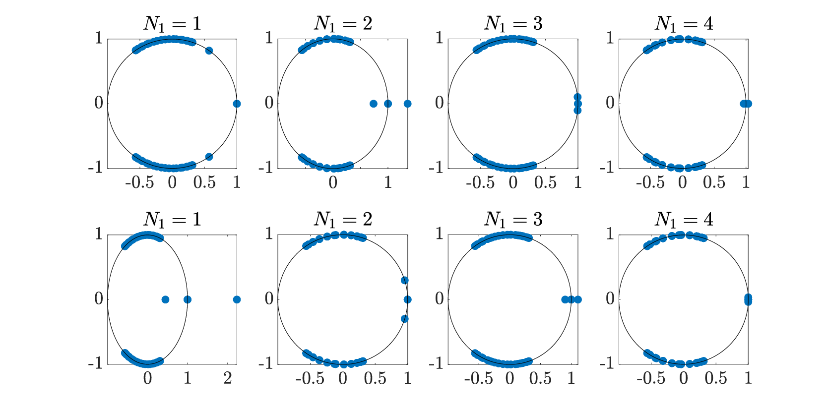
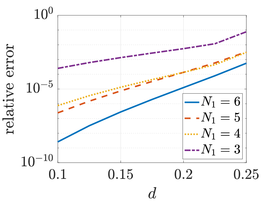
Fig. 16 shows the bifurcation diagram for out-of-phase and in-phase double breathers for $N_{1}=6$ . As noted above, the out-of-phase double breather is spectrally stable, while the in-phase double breather is unstable. For $N_{1}$ odd, this pattern is reversed (not shown). The upper branches are double breathers comprising two out-of-phase inter-site centered breathers, where we recall that this is the unstable configuration for the inter-site centered breather. The middle branch is an asymmetric double breather, comprising one single-site breather and one out-of-phase inter-site centered breather. Fig. 17 shows the relative error in the computation of the Floquet interaction eigenmodes on the lower branches for both the in-phase and out-of-phase double breathers for both even and odd $N_{1}$ , using the formula Eq. 62. As for the sine-Gordon equation, the relative error increases with $d$ . We note that the relative error is less than $10^{-2}$ up to approximately $d=0.25$ , which is close to the turning points of the bifurcation diagrams.

Potential	$N_{1}$	sign of $K$	sign of $b_{1}$	in-phase	out-of-phase
sine-Gordon (soft)	even	$-$	$-$	unstable	stable
	odd	$-$	$-$	unstable	stable
$\phi^{4}$ (hard)	even	$+$	$+$	unstable	stable
	odd	$+$	$-$	stable	unstable

Table 2. Summary of Floquet interaction eigenmode pattern for double breathers for soft sine-Gordon potential and hard

\phi^{4}

potential.

6. Conclusions and future directions

In this paper, we studied multi-breather solutions to the discrete Klein-Gordon equation, with an emphasis on a theoretical analysis of multi-breathers with well-separated excited sites, and their existence, spectral stability and dynamical properties. Specifically, we looked at an approximation of the system on a finite-dimensional Hilbert space, and used Lin’s method to construct multi-breather solutions to this system. Furthermore, we used Lin’s method again to reduce the eigenvalue problem to a low-dimensional, matrix equation, which can then be solved. This can be done as long as the distances between copies of the primary breather are sufficiently large. The results from this approximation are in very good agreement with direct numerical computations of the Floquet spectrum, both for soft and hard potentials. The key determining factor for the Floquet spectral pattern is the phase differences between adjacent copies of the primary, single-site breather. In addition, our results showcased the crucial difference between the soft sine-Gordon equation and the hard $\phi^{4}$ equation; in the latter case, the Floquet spectral pattern depends in addition on whether the distances in lattice points between consecutive copies of the primary breather are even or odd, while in the former case, it does not (see also, e.g., the analogy with the interaction of dark solitons in the defocusing DNLS model of [55]).

Avenues of further research include exploring breathers and multi-breathers either in Klein-Gordon lattices with asymmetric potentials, such as the Morse potential, or in other models involving beyond-nearest-neighbor interactions, discussed, e.g., in [57] and references therein. One class of models which would be interesting to study concerns equations in which the potential involves off-site terms, such as the FPUT lattice. A natural extension of this would be to look at higher dimensional lattices, both for on-site potentials such as in a higher dimensional Klein-Gordon model, and more complex potentials, such as higher dimensional FPUT lattices. In two dimensions, there are many possible regular lattice models, including square, triangular, and honeycomb, and these different geometries may exhibit qualitatively different behavior. Another possibility would be to look at more complex solutions. One class of solutions which remains unexplored is asymmetric multi-breathers, solutions comprising breathers which have different, but commensurate, fundamental periods. Fig. 18(a) shows an example of an asymmetric double breather solution to the discrete sine-Gordon equation; the left breather has a fundamental period of 8, and the right breather has a fundamental period of 16, so the overall breather has a period of 16. While these solutions can be constructed numerically by parameter continuation from the AC limit, preliminary numerical experiments suggest that they only exist for small values of the coupling parameter $d$ , and that they are spectrally unstable. In addition, preliminary numerical experiments suggest that there are solutions comprising both breathers and kinks. See Fig. 18(b) for an example of a solution to the discrete sine-Gordon equation in which a breather is connected to a kink. Finally, although the finite-dimensional approximation used in the paper yields results which are in very good agreement with those found numerically, it may be still possible to remove this restriction and prove the results for the full system, although this would most likely involve an entirely different approach.

Acknowledgments

This material is based upon work supported by the U.S. National Science Foundation under the RTG grant DMS-1840260 (R.P. and A.A.) and DMS-1809074 (P.G.K.). J.C.-M. acknowledges support from EU (FEDER program 2014-2020) through both Consejería de Economía, Conocimiento, Empresas y Universidad de la Junta de Andalucía (under the projects P18-RT-3480 and US-1380977), and MICINN and AEI (under the projects PID2019-110430GB-C21 and PID2020-112620GB-I00). R.P. would also like to thank Graham Cox and Björn Sandstede for their helpful comments and suggestions.

Appendix A Proof of Theorem 2

The proof is a straightforward adaptation of the proof of [53]*Theorem 2. Let $Y(n)=(y(n),\tilde{y}(n))=\omega\partial_{\omega}U(n)$ . We take as an ansatz for the eigenfunction $W(n)$ the following piecewise linear combination

(66)

W_{i}^{\pm}(n)=c_{i}(\dot{U}_{i}^{\pm}(n)+\lambda Y_{i}^{\pm}(n))+\tilde{W}_{i}^{\pm}(n),

where $c_{i}\in{\mathbb{C}}$ , and $W_{i}^{\pm}(n)$ is defined on the same interval as $U_{i}^{\pm}(n)$ in Eq. 48. Substituting Eq. 66 into Eq. 40, using the relations

(67)		$\displaystyle\dot{U}_{i}^{\pm}(n+1)$	$\displaystyle=DF_{M}(U(n))\dot{U}_{i}^{\pm}(n)$
(67)		$\displaystyle\qquad Y_{i}^{\pm}(n+1)$	$\displaystyle=DF_{M}(U(n))Y_{i}^{\pm}(n)+2\partial_{t}B\dot{U}_{i}^{\pm}(n),$

and simplifying, we obtain the equation

(68)		$\displaystyle\tilde{W}_{i}^{\pm}(n+1)$	$\displaystyle=DF_{M}(\sigma_{i}Q_{M}(n))\tilde{W}_{i}^{\pm}(n)+\lambda^{2}c_{i}B[2\partial_{t}Y_{i}^{\pm}(n)+\dot{U}_{i}^{\pm}(n)]$
(68)			$\displaystyle+[G_{i}^{\pm}(n)+(2\lambda\partial_{t}+\lambda^{2})B]\tilde{W}_{i}^{\pm}(n)+c_{i}\lambda^{3}BY_{i}^{\pm}(n),$

where

(69)

G_{i}^{\pm}(n)=DF_{M}(U_{i}^{\pm}(n))-DF_{M}(\sigma_{i}Q_{M}(n)).

In addition to solving Eq. 68, the eigenfunction $W_{i}^{\pm}$ must satisfy matching conditions at $n=\pm N_{i}$ and $n=0$ . As in [53, 52, 59], this will in general not be possible. Instead, we solve the system

(70)	$\displaystyle\tilde{W}_{i}^{\pm}(n+1)$	$\displaystyle=DF_{M}(\sigma_{i}Q_{M}(n))\tilde{W}_{i}^{\pm}(n)+\lambda^{2}c_{i}B[2\partial_{t}Y_{i}^{\pm}(n)+\dot{U}_{i}^{\pm}(n)]$
		$\displaystyle+[G_{i}^{\pm}(n)+(2\lambda\partial_{t}+\lambda^{2})B]\tilde{W}_{i}^{\pm}(n)+c_{i}\lambda^{3}BY_{i}^{\pm}(n)$
	$\displaystyle\tilde{W}_{i}^{+}(N_{i}^{+})$	$\displaystyle-\tilde{W}_{i+1}^{-}(-N_{i}^{-})=C_{i}c$
	$\displaystyle\tilde{W}_{i}^{+}(0)$	$\displaystyle-\tilde{W}_{i}^{-}(0)\in{\mathbb{C}}Z_{M}(n),$

where

(71)

\displaystyle C_{i}c

\displaystyle=[\dot{U}_{i+1}^{-}(-N_{i}^{-})+\lambda Y_{i+1}^{-}(-N_{i}^{-})]c_{i+1}-[\dot{U}_{i}^{+}(N_{i}^{+})+\lambda Y_{i}^{+}(N_{i}^{+})]c_{i}.

A solution to Eq. 70 is an eigenfunction if and only if the $m$ jump conditions

(72)

\displaystyle\xi_{i}

\displaystyle=\langle\sigma_{i}Z_{M}(0),\tilde{W}_{i}^{+}(0)-\tilde{W}_{i}^{-}(0)\rangle=0

\displaystyle i=1,\dots,m

are satisfied.

We proceed as in the proof of [53]*Theorem 2. Since $DF_{M}(0)$ is hyperbolic, and

\|Q_{M}(n)\|_{L^{2}_{\textrm{per}}([0,T])}\leq Cr_{M}^{-|n|}

by the stable manifold theorem, we can adapt the results of [50] to decompose the evolution operator $\Phi(m,n)$ of the variational equation Eq. 43 in exponential dichotomies on ${\mathbb{Z}}^{\pm}$ . We then rewrite Eq. 68 as a fixed point problem using the discrete variation of constants formula (see, for example, [53]*Lemma 3), and project onto the stable and unstable subspaces of the exponential dichotomy. From there, we follow the steps in [53], using the estimates Eq. 51, to obtain a unique solution to Eq. 70. The jump conditions Eq. 72 become

(73)	$\displaystyle\xi_{i}$	$\displaystyle=\sigma_{i}\sigma_{i+1}\langle Z_{M}(N_{i}^{+}),\dot{Q}_{M}(-N_{i}^{-})\rangle(c_{i+1}-c_{i})$
		$\displaystyle+\sigma_{i}\sigma_{i-1}\langle Z_{M}(-N_{i-1}^{-}),\dot{Q}_{M}(N_{i-1}^{+})\rangle(c_{i}-c_{i-1})$
		$\displaystyle-\frac{1}{d}\lambda^{2}\sum_{n=-\infty}^{\infty}\left\langle Z_{M}(n+1),B[2\partial_{t}Y(n)+\dot{Q}_{M}(n)]\right\rangle+R(\lambda)_{i}(c),$

where the remainder term has the uniform bound

\|R(\lambda)(c)\|_{X_{M}^{2}}\leq C\left(r_{M}^{-N}+|\lambda|\right)^{3}.

Evaluating the inner products, we obtain for the jumps

(74)

\displaystyle\xi_{i}

\displaystyle=a_{i}(c_{i+1}-c_{i})+\tilde{a}_{i-1}(c_{i}-c_{i-1})+\frac{1}{d}\lambda^{2}K+R(\lambda)_{i}(c),

where $a_{i}$ and $\tilde{a}_{i-1}$ are defined by Eq. 54, and $K$ is defined by Eq. 55. Equation Eq. 52 follows by writing the jump conditions Eq. 74 in matrix form as

(75)

\left(A+\frac{1}{d}K\lambda^{2}I+R(\lambda)\right)c=0

on ${\mathbb{R}}^{m}$ , where $c=(c_{1},\dots,c_{m})^{T}$ , and the matrix $A$ is defined by Eq. 53. Equation Eq. 75 has a nontrivial solution if and only if its determinant is 0.

References

[1] M. J. Ablowitz and J. F. Ladik (1975) Nonlinear differential-difference equations. Journal of Mathematical Physics 16 (3), pp. 598–603. External Links: Link Cited by: §4.1.
[2] M. J. Ablowitz and J. F. Ladik (1976) Nonlinear differential–difference equations and Fourier analysis. Journal of Mathematical Physics 17 (6), pp. 1011–1018. Cited by: §4.1.
[3] M. J. Ablowitz and H. Segur (2000) Solitons and the inverse scattering transform. 1 edition, SIAM Studies in Applied Mathematics, No. 4, Society for Industrial Mathematics. External Links: ISBN 9780898714777,089871477X Cited by: §1.
[4] A. B. Aceves, L. A. Cisneros-Ake, and A. A. Minzoni (2011) Asymptotics for supersonic traveling waves in the morse lattice. Discrete and Continuous Dynamical Systems - S 4 (5), pp. 975–994. Cited by: §1.
[5] T. Ahn, R. S. MacKay, and J. A. Sepulchre (2001) Dynamics of relative phases: generalised multibreathers. Nonlinear Dynamics 25, pp. 157–182. Cited by: §1.
[6] A. A. Aigner, A.R. Champneys, and V. M. Rothos (2003) A new barrier to the existence of moving kinks in Frenkel–Kontorova lattices. Physica D: Nonlinear Phenomena 186. Cited by: §1.
[7] J. F. R. Archilla, J. Cuevas, B. Sánchez-Rey, and A. Alvarez (2003) Demonstration of the stability or instability of multibreathers at low coupling. Physica D: Nonlinear Phenomena 180. Cited by: §1, §5.1, §5.2.
[8] G. Arioli and H. Koch (2019) Some breathers and multi-breathers for FPU-type chains. Communications in Mathematical Physics 372, pp. 1117–1146. Cited by: §1.
[9] S. Aubry (1997) Breathers in nonlinear lattices: existence, linear stability and quantization. Physica D: Nonlinear Phenomena 103. Cited by: §1.
[10] D. Bambusi (2013) Asymptotic stability of breathers in some Hamiltonian networks of weakly coupled oscillators. Communications in Mathematical Physics 324. Cited by: §1.
[11] W. J. Beyn (1990) The numerical computation of connecting orbits in dynamical systems. IMA Journal of Numerical Analysis 10 (3), pp. 379–405. Cited by: §5.
[12] J. J. Bramburger, J. Cuevas-Maraver, and P. G. Kevrekidis (2020) Vortex pairs in the discrete nonlinear Schrödinger equation. Nonlinearity 33. Cited by: §5.1.
[13] O. M. Braun and Y. S. Kivshar (1998) Nonlinear dynamics of the Frenkel-Kontorova model. Physics Reports 306 (1-2), pp. 1–108 (en). External Links: ISSN 03701573 Cited by: §1.
[14] O. M. Braun and Y. S. Kivshar (2004) The Frenkel-Kontorova Model. Springer Berlin Heidelberg, Berlin, Heidelberg. Cited by: §1, §1.
[15] A. R. Champneys and G. J. Lord (1997) Computation of homoclinic solutions to periodic orbits in a reduced water-wave problem. Physica D: Nonlinear Phenomena 102 (1), pp. 101–124. Cited by: §5.
[16] M. Chirilus-Bruckner, C. Chong, J. Cuevas-Maraver, and P. G. Kevrekidis (2014) sine-Gordon equation: from discrete to continuum. pp. 31–57. Cited by: §1, §1.
[17] L. A. Cisneros and A. A. Minzoni (2008) Asymptotics for kink propagation in the discrete sine-Gordon equation. Physica D: Nonlinear Phenomena 237. Cited by: §1.
[18] J. Cuevas, L. Q. English, P. G. Kevrekidis, and M. Anderson (2009) Discrete breathers in a forced-damped array of coupled pendula: modeling, computation, and experiment. Phys. Rev. Lett. 102, pp. 224101. External Links: Link Cited by: §1.
[19] J. Cuevas, V. Koukouloyannis, P. G. Kevrekidis, and J. F. R. Archilla (2011) Multibreather and vortex breather stability in klein-gordon lattices: equivalence between two different approaches. International Journal of Bifurcation and Chaos 21 (08), pp. 2161–2177. Cited by: §1.
[20] J. Cuevas-Maraver and P. G. K. (eds.) (2019) A dynamical perspective on the $\phi^{4}$ model. 1 edition, Nonlinear Systems and Complexity, Springer International Publishing. External Links: ISBN 978-3030118389 Cited by: §1, §1.
[21] J. Cuevas-Maraver, P. G. Kevrekidis, and F. L. W. (eds.) (2014) The sine-Gordon model and its applications: from pendula and Josephson junctions to gravity and high-energy physics. 1 edition, Nonlinear Systems and Complexity 10, Springer International Publishing. External Links: ISBN 978-3-319-06721-6,978-3-319-06722-3 Cited by: §1, §1.
[22] J. Cuevas-Maraver, P. G. Kevrekidis, and D. E. Pelinovsky (2016) Nonlinear instabilities of multi-site breathers in Klein-Gordon lattices. Studies in Applied Mathematics 137 (2), pp. 214–237. External Links: ISSN 00222526 Cited by: §1, §1, §1, §2.1, §2.3, §2.3, §2, §5.1, §5.1, §5.2.
[23] E. J. Doedel, T. F. Fairgrieve, B. Sandstede, A. R. Champneys, Y. A. Kuznetsov, and X. Wang (2007) AUTO-07P: continuation and bifurcation software for ordinary differential equations. Cited by: §5.
[24] C. Elphick, E. Meron, and E. A. Spiegel (1990) Patterns of propagating pulses. SIAM Journal on Applied Mathematics 50 (2), pp. 490–503. Cited by: §1.
[25] E. Fermi, P. Pasta, S. Ulam, and M. Tsingou Studies of the nonlinear problems. External Links: Link Cited by: §1.
[26] S. Flach and C. R. Willis (1998) Discrete breathers. Physics Reports 295. Cited by: §1.
[27] S. Flach and A. V. Gorbach (2008) Discrete breathers — advances in theory and applications. Physics Reports 467. Cited by: §1.
[28] S. Flach and A. Gorbach (2008) Discrete breathers with dissipation. Vol. 751, pp. 1–32. Cited by: §1.
[29] L. M. Floría, J. L. Marín, S. Aubry, P. J. Martínez, F. Falo, and J. J. Mazo (1998) Josephson-junction ladder: a benchmark for nonlinear concepts. Physica D: Nonlinear Phenomena 113 (2), pp. 387–396. External Links: ISSN 0167-2789, Link Cited by: §1.
[30] E. Hairer and M. Hairer (2003) GniCodes — Matlab programs for geometric numerical integration. In Frontiers in numerical analysis, J. F. Blowey, A. W. Craig, and T. Shardlow (Eds.), pp. 199–240 (en). External Links: Link Cited by: §5.1.
[31] E. Hairer, C. Lubich, and G. Wanner (2006) Geometric numerical integration. Springer Series in Computational Mathematics, Vol. 31, Springer-Verlag, Berlin/Heidelberg (en). External Links: ISBN 9783540306634, Link Cited by: §5.1.
[32] D. Hennig (2021) Localised time-periodic solutions of discrete nonlinear Klein-Gordon systems with convex on-site potentials. Journal of Fixed Point Theory and Applications 23 (2), pp. 31. External Links: ISSN 1661-7738, 1661-7746 Cited by: §1.
[33] G. Iooss and D. E. Pelinovsky (2006) Normal form for travelling kinks in discrete Klein–Gordon lattices. Physica D: Nonlinear Phenomena 216. Cited by: §1.
[34] G. Kalosakas (2006) Multi-peaked localized states of DNLS in one and two dimensions. Physica D: Nonlinear Phenomena 216 (1), pp. 44–61. Note: Nonlinear Physics: Condensed Matter, Dynamical Systems and Biophysics External Links: ISSN 0167-2789, Link Cited by: §1.
[35] T. Kapitula and P. Kevrekidis (2001) Stability of waves in discrete systems. Nonlinearity 14 (3), pp. 533–566. Cited by: §4.1.
[36] T. Kapitula and K. Promislow (2013) Spectral and dynamical stability of nonlinear waves. Springer New York. Cited by: §2.2.
[37] N. Karachalios (2005) Global existence in infinite lattices of nonlinear oscillators: the discrete Klein-Gordon equation. Glasgow Mathematical Journal 48. Cited by: §1.
[38] P. G. Kevrekidis, D. E. Pelinovsky, and A. Saxena (2015) When linear stability does not exclude nonlinear instability. Phys. Rev. Lett. 114, pp. 214101. External Links: Link Cited by: §1.
[39] P. G. Kevrekidis and M. I. Weinstein (2000) Dynamics of lattice kinks. Physica D: Nonlinear Phenomena 142 (1-2), pp. 113–152 (en). External Links: ISSN 01672789, Link Cited by: §1, §2.
[40] P. G. Kevrekidis (2011) Non-linear waves in lattices: past, present, future. IMA Journal of Applied Mathematics 76 (3), pp. 389–423. External Links: ISSN 0272-4960 Cited by: §1.
[41] P. G. Kevrekidis, J. Cuevas-Maraver, and D. E. Pelinovsky (2016) Energy criterion for the spectral stability of discrete breathers. Physical Review Letters 117 (9), pp. 094101. External Links: ISSN 0031-9007, 1079-7114 Cited by: §2.2, Remark 1.
[42] P. G. Kevrekidis (2009) The discrete nonlinear Schrödinger equation. Springer Berlin Heidelberg. Cited by: §5.1.
[43] Y. S. Kivshar and B. A. Malomed (1989) Dynamics of solitons in nearly integrable systems. Rev. Mod. Phys. 61, pp. 763–915. Cited by: §1, §1.
[44] J. Knobloch (2000) Lin’s method for discrete dynamical systems. Journal of Difference Equations and Applications 6 (5), pp. 577–623. Cited by: §1, §4.2.
[45] V. Koukouloyannis and P. G. Kevrekidis (2009) On the stability of multibreathers in Klein–Gordon chains. Nonlinearity 22. Cited by: §1, §5.1, §5.2.
[46] V. Koukouloyannis (2013) Non-existence of phase-shift breathers in one-dimensional Klein–Gordon lattices with nearest-neighbor interactions. Physics Letters A 377 (34), pp. 2022–2026. External Links: ISSN 0375-9601, Link Cited by: §2.1, §4.2.
[47] F. Lederer, G. I. Stegeman, D. N. Christodoulides, G. Assanto, M. Segev, and Y. Silberberg (2008) Discrete solitons in optics. Physics Reports 463 (1), pp. 1–126. External Links: ISSN 0370-1573, Link Cited by: §1.
[48] R. D. Leo and S. Demelio (2011) Some numerical results on motion of kinks in some model of DNA torsional dynamics. Communications in Applied and Industrial Mathematics 2 (1). External Links: ISSN 20380909 Cited by: §1.
[49] R. S. MacKay and S. Aubry (1994) Proof of existence of breathers for time-reversible or hamiltonian networks of weakly coupled oscillators. Nonlinearity 7. Cited by: §1.
[50] K. J. Palmer (1988) Exponential dichotomies, the shadowing lemma and transversal homoclinic points. In Dynamics reported, pp. 265–306. External Links: Link Cited by: Appendix A.
[51] A. Pankov (2005) Travelling waves and periodic oscillations in Fermi-Pasta-Ulam lattices. External Links: ISBN 1860945325 Cited by: §1.
[52] R. Parker, P. G. Kevrekidis, and A. Aceves (2022) Stationary multi-kinks in the discrete sine-Gordon equation. Nonlinearity 35, pp. 1036–1060. Cited by: Appendix A, §1, §1, §2.4, §2.4, §4.2, §4, §5.1, Theorem 1.
[53] R. Parker, P. G. Kevrekidis, and B. Sandstede (2020) Existence and spectral stability of multi-pulses in discrete Hamiltonian lattice systems. Physica D: Nonlinear Phenomena 408, pp. 132414 (en). External Links: ISSN 01672789 Cited by: Appendix A, Appendix A, Appendix A, Appendix A, §1, §1, §1, §2.4, §2.4, §4.1, §4.2, §4.3, §4, Corollary 1, Theorem 1.
[54] D. E. Pelinovsky, P. G. Kevrekidis, and D. J. Frantzeskakis (2005) Stability of discrete solitons in nonlinear Schrödinger lattices. Physica D: Nonlinear Phenomena 212. Cited by: §1.
[55] D. E. Pelinovsky and P. G. Kevrekidis (2008) Stability of discrete dark solitons in nonlinear Schrödinger lattices. Journal of Physics A: Mathematical and Theoretical 41 (18), pp. 185206. External Links: Link Cited by: §6.
[56] D. Pelinovsky and A. Sakovich (2012) Multi-site breathers in Klein-Gordon lattices: stability, resonances and bifurcations. Nonlinearity 25 (12), pp. 3423–3451. External Links: Link Cited by: §1, §1, §1, §2.1, §2.1, §2.1, §2.2, §4.2, §4.3, §4, Remark 1.
[57] T. Penati, V. Koukouloyannis, M. Sansottera, P. G. Kevrekidis, and S. Paleari (2019) On the nonexistence of degenerate phase-shift multibreathers in Klein–Gordon models with interactions beyond nearest neighbors. Physica D: Nonlinear Phenomena 398, pp. 92–114. External Links: ISSN 0167-2789, Link Cited by: §2.1, §6.
[58] M. Peyrard and M. D. Kruskal (1984) Kink dynamics in the highly discrete sine-Gordon system. Physica D: Nonlinear Phenomena 14 (1), pp. 88–102. External Links: ISSN 0167-2789 Cited by: §1.
[59] B. Sandstede (1998) Stability of multiple-pulse solutions. Transactions of the American Mathematical Society 350 (02), pp. 429–473. Cited by: Appendix A, §1, §2.4, §4.2, §4.3, §4.3, §4.
[60] A. C. Scott (1969) A nonlinear Klein-Gordon equation. American Journal of Physics 37 (1), pp. 52–61. Cited by: §1.
[61] A. V. Ustinov, T. Doderer, R. P. Huebener, N. F. Pedersen, B. Mayer, and V. A. Oboznov (1992) Dynamics of sine-Gordon solitons in the annular Josephson junction. Phys. Rev. Lett. 69, pp. 1815–1818. External Links: Link Cited by: §1.
[62] L. V. Yahushevich (1998) Nonlinear physics of DNA. Wiley series in nonlinear science, John Wiley Sons, Chichester, New York. External Links: ISBN 9780471978244 Cited by: §1.
[63] S. Yomosa (1983) Soliton excitations in deoxyribonucleic acid (DNA) double helices. Phys. Rev. A 27, pp. 2120–2125. Cited by: §1.
[64] K. Yoshimura and Y. Doi (2021) Existence of odd, even, and multi-pulse discrete breathers in infinite Fermi-Pasta-Ulam lattices. Journal of Differential Equations 298, pp. 560–608. External Links: ISSN 00220396 Cited by: §1.
[65] N. J. Zabusky and M. D. Kruskal (1965) Interaction of “solitons” in a collisionless plasma and the recurrence of initial states. Phys. Rev. Lett. 15, pp. 240–243. External Links: Link Cited by: §1.

Revisiting Multi-breathers in the discrete Klein-Gordon equation: A Spatial Dynamics Approach

Abstract.

1. Introduction

2. Mathematical background

2.1. Breathers

2.2. Linearization

2.3. Continuous spectrum

2.4. Spatial dynamics

2.5. Spectrum of D​F​(0)DF(0)

Lemma 1.

Proof.

Lemma 2.

Proof.

Hypothesis 1.

3. Finite dimensional approximation

4. Multi-breathers

4.1. Primary breather

Hypothesis 2.

Hypothesis 3.

4.2. Existence

Theorem 1.

Proof.

4.3. Spectral stability

Theorem 2.

Remark 1.

Corollary 1.

Proof.

5. Numerical results

5.1. Discrete sine-Gordon equation

5.2. Hard ϕ4\phi^{4} potential

6. Conclusions and future directions

Acknowledgments

Appendix A Proof of Theorem 2

References

2.5. Spectrum of $DF(0)$

5.2. Hard $\phi^{4}$ potential