Quantum dynamics corresponding
to chaotic BKL scenario
Abstract
We quantize the solution to the Belinski-Khalatnikov-Lifshitz (BKL) scenario using the integral quantization method. Quantization smears the gravitational singularity avoiding its localization in the configuration space. The latter is defined in terms of spatial and temporal coordinates, which are treated on the same footing that enables respecting covariance of general relativity. The relative quantum perturbations grow as the system evolves towards the gravitational singularity. The quantum randomness amplifies the deterministic classical chaos of the BKL scenario. Additionally, our results suggest that the generic singularity of general relativity can be avoided at quantum level giving support to the expectation that quantum gravity has good chance to be a regular theory.
I Introduction
The Belinski, Khalatnikov and Lifshitz (BKL) conjecture states that general relativity includes the solution with generic gravitational singularity BKL2; BKL3. The evolution towards the BKL singularity, the so-called BKL scenario, consists of the deterministic dynamics turning into stochastic process near the generic singularity. There are at least two fundamental questions to be addressed in that context: What is the fate of the BKL chaos at quantum level? Can the singularity be avoided in the corresponding quantum theory?
The evolution process presented in BKL2; BKL3 is complicated and difficult to map into quantum evolution. There exists well defined and comparatively simple model of the BKL scenario bkl; Belinski:2014kba; book that can be used in the derivation of the BKL conjecture private. The model has been obtained from the general model of the Bianchi IX spacetime for perfect fluid. The equation of state of that fluid reads where and denote the pressure and energy density of the fluid, respectively. The case is excluded as it does not lead to the oscillatory dynamics specific to the Bianchi IX model. The massive BKL scenario model has been obtained from that general Bianchi IX model by making the assumption (see Eq. (3)) that in the dynamics, near the singularity, the anisotropy of space grows without bound so that each of the so-called directional scale factors oscillate, but never crosses each other, and evolves towards vanishing, i.e., singularity. The resulting dynamics, specified in the next section, is different from the commonly known mixmaster dynamics Volodia; mix in which one can divide the oscillatory evolution of the system into eras, each consisting of Kasner’s epochs, evolving towards the singularity. The mixmaster model is the vacuum Bianchi IX model and can serve to derive the BKL conjecture as well private so that we call it the vacuum model of the BKL scenario. We have made the comparison of the dynamics of both massive and vacuum models within dynamical systems method recently ECz. The dynamics of the massive BKL model depends on the matter field implicitly via the directional scale factors which are effective ones, see Eqs. (2.6), (2.7) and (2.24) in bkl. Also, due to the dependence of the general Bianchi IX model on matter components, it was possible to obtain the asymptotic form (near the singularity) of the general dynamics bkl. That dynamics is mathematically simple enough to be solved analytically Piotr. The dynamics of the vacuum Bianchi IX model is the same faraway and near the singularity. It is so complex that the model is non-integrable Conte. Therefore, the massive BKL model is both simpler for analysis than the vacuum BKL model, and better suitable to describe the dynamics in the neighborhood of the cosmological singularity.
Recently, we have verified numerically that the classical dynamics underlying the present paper leads to the gravitational singularity Nick1; Nick2, and it is generically unstable turning into chaotic process near the singularity Piotr. These features are consistent with the original BKL scenario BKL2; BKL3; book.
As far as we are aware, there are not available any results concerning the issue of the construction of quantum theory corresponding directly to the original BKL scenario BKL2; BKL3. The existing results concern the Hamiltonian framework, in terms of Ashtekar’s variables, that is supposed to be convenient to address the BKL scenario problem David1; David2. We have used the homogeneous sector of that formalism to consider the possibility of existence of classical end quantum spikes within that sector WPa; WPb. Recent article on spacelike singularities of general relativity makes promise of coming back to the issue of addressing the original BKL singularity problem within loop quantum gravity Abhay. We do not exclude the case of joining that development in the future, but presently we rather prefer to follow our programme.
Quantization of the dynamics presented in bkl can be used in the examination of the fate of the corresponding quantum dynamics. In fact, we have already quantized that model with the conclusion that quantization of the dynamics leads to avoiding gravitational singularity AWG; AW. In these papers, we have quantized Hamilton’s dynamics derived in Ewa. However, since quantization is known to be an ambiguous procedure, we have decided to examine the robustness of these results by making use of a completely different quantization method, which is one of the goals of the present paper. That method, applied recently to the quantization of the Schwarzschild spacetime AOW, includes quantization of the temporal and spatial variables on the same footing. The rationale for such dealing is that the distinction between time and space variables violates the general covariance of arbitrary transformations of temporal and spatial coordinates.
The results of the present paper, in the context of resolving the cosmological singularity, are similar to the results of the paper AOW addressing the issue of a singularity of an isolated object. In both cases quantization smears the singularity avoiding its localization in configuration space. The issue of resolving the singularity within our two quite different approaches will be further discussed in the last section.
The new phenomenon we deal with, in the present paper, is the fate of the classical chaos at quantum level. Our analysis shows that the quantum randomness turns deterministic classical chaos into stochastic quantum chaos.
The paper is organized as follows: In Sec. II we recall the main results of the paper Piotr to have our paper self-contained. Sec. III presents the main aspects of the coherent states quantization method adopted to our gravitational system. In Sec. IV we quantize the solution to the BKL scenario. Stochastic aspects of quantum evolution are presented in Sec. V. We conclude in the last section. Appendix presents the essence of the coherent states quantization.
In the following we choose except where otherwise noted.
II Solution to the BKL scenario
To have the paper self-contained, we recall in this section the main results of Ref. Piotr to be used later.
The massive model of the BKL scenario is defined to be bkl; book
| (1) |
subject to the constraint
| (2) |
where and are the so-called directional scale factors, while is a monotonic function of proper time.
Eqs. (1)–(2) have been derived from the general dynamics of the Bianchi IX model under the condition that near the singularity the following strong inequalities are satisfied bkl
| (3) |
It has been found in Piotr that the analytical solutions to Eqs. (1)–(2), for , read
| (4) |
where and is an arbitrary real number. Thus, the solutions are parameterized by the number .
The solution (4) corresponds, for instance in the case and , to the following choice of the initial data
| (5) | ||||||
The stability analyses carried out in Piotr have shown that the solution (4) is unstable against small perturbation. More precisely, substituting the following functions
| (6a) | ||||
| (6b) | ||||
| (6c) | ||||
into (1)–(2) leads, in the first order in the small parameter , to the following solution of the resulting equations
| (7a) | ||||
| (7b) | ||||
| (7c) | ||||
where . The two frequencies read
| (8) |
where and are constants.
The manifold defined by is a submanifold of . The solution defined by (6) and (7) corresponds to the choice of the set of the initial data that is a small neighborhood of the initial data (II). is a submanifold of as (II) defines five independent constants due to the constraint (2). Therefore, it is clear that (7) presents a generic solution as the measures of both and are nonzero. The exact solution (4) alone is of zero-measure in the space of all possible solutions to Eqs. (1)–(2).
The relative perturbations and grow proportionally as . The multiplier plays the role of a Lyapunov exponent, describing the rate of their divergence. Since it is positive, the evolution of the system towards the gravitational singularity () is chaotic. The transition into the chaos occurs if the evolution begins with the initial data which belong, for instance, to the neighbourhood of the conditions (II).
The original BKL scenario BKL2; BKL3 is known to enter the chaotic phase near the singularity. Its vacuum model, the mixmaster universe, has been proved to include the chaotic dynamics st1; st2; st3; st4; st5. Its massive model Piotr, underlying the present paper, has never been examined earlier in the context of stochasticity. Finding that its dynamics is chaotic, opens the door for studies of that issue at quantum level, which is the main subject of our article. The main difference between both BKL models (in terms of physics) is that the latter is more realistic near the singularity as it includes effectively some contribution from matter field.
III Affine coherent states quantization
We propose to quantize the classical BKL scenario by using the integral quantization called the affine coherent states quantization, see Appendix. We have recently applied this approach in the context of cosmology AWG; AW and astrophysics AOW; WPTS.
In general relativity time and position in space are treated on the same level, however, in quantum mechanics time is not considered to be a quantum observable, but a parameter enumerating events. In this paper, we treat time and position on the same footing in the quantum description. They are related to operators obtained by the affine coherent states quantization. This idea requires introducing the notion of an extended classical configuration space by including time as an additional coordinate. The correspondence between the classical time and position is done by comparing their classical values with expectation values of their quantum counterparts.
In the following, we extend the method of quantization used in AWG; AW; AOW. In the present description of the BKL scenario, the Hilbert space has to be extended to the carrier space of infinite dimensional unitary irreducible representation of the direct product of three affine groups with additional constraints determining a model of physical time. In this approach there is no distinction between kinematical and dynamical Hilbert spaces; we construct the state space of the system with time treated on the same footing as other observables. In addition, we obtain quantum states evolving similarly to classical solutions. It is achieved by using the idea of the correspondence principle between quantum mechanics and its classical approximation.
To begin with, we introduce two configuration spaces defined as follows: the classical gravitational configuration space
| (9) |
where , and the affine configuration space is defined as
| (10) |
where every pair , (), parameterizes the affine group .
The variables with even indices correspond to the scale factors . Because and , the configuration space parametrizes the simple product of 3 affine groups to be used in the affine quantization.
As the observational data are parameterized by a single time parameter, the variables should be mapped onto a single variable representing time.
The affine group is known to have two nontrivial unitary irreducible representations in the Hilbert space , where . We choose the one defined as follows (the second representation would give exactly the same results):
| (11) |
where, and . The action (11) corresponds to the standard parametrization of the affine group defined by the multiplication law
| (12) |
The left invariant measure on the group reads
| (13) |
and the corresponding invariant integration over the affine group is defined to be
| (14) |
It is clear that the direct product of three affine groups has the unitary irreducible representation in the following Hilbert space , where . It enables defining in the continuous family of affine coherent states , as follows
| (15) |
where , and and where
| (16) |
In (16) the vectors , are the so-called fiducial vectors. They are required to satisfy the two conditions
| (17) |
and
| (18) |
where for , for and for . The fiducial vectors are the free “parameters” of this quantization scheme.
Finally, we have
| (19) |
The irreducibility of the representation leads to the resolution of the unity in as follows
| (20) |
where .
The resolution (III) can be used for mapping a classical observable into an operator as follows AWG; AW; AWT; AOW
| (21) |
where .
Here, we recall two standard characteristics of quantum observables: (i) expectation values and variances of quantum observables are the most important characteristics which allow to compare quantum and classical worlds, and (ii) expectation values of quantum observables correspond to classical values of measured quantities and their variances describe quantum smearing of these observables.
A general form of expectation value of the observable obtained from the classical function , while the quantum system is in the state , reads
| (22) |
The variance of an observable defined as is more difficult for calculations because it requires which involves an overlap between the coherent states, and usually depends on the fiducial vector explicitly:
| (23) |
The variance can be rewritten as
| (24) |
The important quantum observables correspond to the variables of the configuration space (10). These elementary variables (), can be mapped into the quantum operators as follows
| (25) |
For every the above equality (25) reduces to integration over a single affine group. The other integrations give the unit operators in two remaining spaces , . For example,
| (26) |
To deal with a single time variable at quantum level, one needs to choose a model of time in the configuration space , defined by (10). In general, it can be introduced either as a real function or distribution, . Its quantization leads to the time operator . However, we can impose the appropriate constraints to have the common time variable for all three operators , and . In this paper we realise that option assuming that the only allowed quantum states of our BKL system are the states which satisfy the condition
| (27) |
which is consistent with the choice of the configuration space in the form (9). It means, we require the same expectation values for all three operators which represent three “times” related to appropriate quantum observables , and .
IV Quantization of the solution to BKL scenario
The above quantization scheme can be now applied to the solutions (7) of the BKL scenario11 1 In what follows we denote by and the solution (4).
| (28) |
ascribing to them appropriate quantum states and the corresponding operators.
In quantum mechanics, contrary to classical one, one needs two kinds of objects to describe physical world. These are quantum observables represented by either appropriate operators or operator valued measures, and quantum states being the vectors in a Hilbert space or the so called density operators. In the classical mechanics the functions on either configuration or phase space are at the same time states and observables.
To quantize solutions of the BKL scenario, we already have the elementary observables . However, we also have to find the appropriate family of states related to the solutions (28). This family of states has to reproduce the classical solutions (28) by comparing them with expectation values of the corresponding observables.
The classical solutions are represented by three time dependent functions. In the configuration space we have 6 variable, where 3 of them represent the time in the state space which satisfies the condition (27). As is it was mentioned above, the classical observables should be related to their quantum counterparts by the corresponding expectation values. This idea leads directly to the conditions for a family of states parameterized by a set of evolution parameters enumerating the set of trial functions.
We require the states to satisfy the following conditions AOW:
| (29) | |||
| (30) | |||
| (31) | |||
| (32) |
The equations (29) represent the single time constraint (27). The parameter labels the family of states to be found, and it should be a function of as the r.h.s. of (29)–(32) depends on . The solution of Eqs. (29)–(32) allows to construct the vector state dependent on classical time, , in our Hilbert space.
In this way we relate the quantum dynamics to the classical one. Obviously, there may exist more than one family of states satisfying the above equations of motion.
In what follows, we determine the states satisfying the conditions (29)–(32). This will enable examination of the issue of the fate of the gravitational singularity and chaos of the BKL scenario at the quantum level.
IV.1 Evolving wave packets
In our paper we consider two kinds of wave packets satisfying the conditions (29)–(32). The first kind are the affine coherent states themselves. The second type is a set of modified “exponential” wave packets, which represent a dense set of states in the Hilbert space .
IV.1.1 Coherent states and expectation values
One can verify that considered coherent states generated by a single affine group satisfy, due to the results of the recent paper AOW, the following equations
| (33) |
where the operators are defined to be
| (34) |
and where , .
The conditions (33) are the consistency conditions between the affine group parametrization and the configuration space of the quantized physical system AOW.
This implies that the coherent states generated by the product of three affine groups also satisfy the consistency condition
| (35) |
The consistency conditions coincide with an idea that the coherent state represents a state localized at the point of the affine configuration space and at the same time in the spacetime.
Therefore, the coherent states
| (36) |
satisfy the equations of motions (29)–(32). In such case, we propose to use a one dimensional parameter and identify it with the classical time , i.e., the classical time is a label of the evolving family of quantum states.
Realization of (36) as a wave packet constructed in the space of square integrable functions reads
| (37) |
IV.1.2 The modified exponential packet and expectation values
Let us consider the set of Gaussian distribution wave packets (with modified exponential part)
| (40) |
which according to AOW is dense in .
The expectation values and variances of the operators and have the following values
| (41) | |||
| (42) | |||
| (43) | |||
| (44) |
In this case, the evolution parameters consists of and .
In the space we take the corresponding wave packets in the form
| (45) |
To meet the properties (29)–(32) for the wave packets , we choose the parameters and as follows
| (46) | |||
| (47) |
where
| (48) |
Using similar technique as in case equation (39), one can calculate the expectation value of the volume operator in the state (45) and one gets
| (49) |
which coincides with the result obtained within coherent states method (39).
It is clear that the expectation value of the volume operator converges very fast to zero as .
IV.2 Variances in the Hilbert space
The wave packets obtained above follow the classical solutions. However, in quantum mechanics the observables which do not commute with time and position operators fluctuate at every spacetime point. This smearing of quantum observables is determined by the Heisenberg uncertainty principle. The most important ingredients of it are variances of the corresponding observables. In the following we perform analysis of the variances of our elementary variables.
IV.2.1 Using coherent states
The variance of the operators , , in coherent states (36) read
| (50) | |||
| (51) |
where
| (52) |
and where is a constant which depends on the choice of the fiducial vector.
The variance of the volume operator is found to be
| (53) |
IV.2.2 Using exponential wave packet
The corresponding results for the wave packets (45), under the conditions (46)-(47), read
| (54) | |||
| (55) |
where
| (56) | |||
| (57) |
The variance of the volume operator has the form
| (58) |
These results show that all positions of our system in time and space are smeared owing to nonzero variances. It is an important fact about possibility of avoiding singularities in this dynamics.
V Stochastic aspects of quantum evolution
The results of recent paper Piotr give strong support to the expectation that near the generic gravitational singularity the evolution becomes chaotic. In what follows we examine that fundamental property of the BKL scenario at quantum level.
To make direct comparison with the results of Piotr, we split the variances (55) into the contributions from unperturbed and perturbed states. We have:
| (59) | |||||
| (60) | |||||
| (61) |
The corresponding dimensionless functions describing relative quantum perturbations are defined to be
| (62) |
where and denote perturbed and unperturbed wave packets, respectively.
The explicit form of (62), up to the 1-st order in , reads:
| (63) | |||||
| (64) | |||||
| (65) |
It is clear that the relative perturbations (63)–(65) are the same for the coherent states and the exponential wave packets.
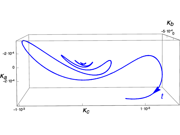
Figure 1 presents the parametric curve visualizing the relative quantum perturbations. The time dependence of the expectation values of operator and corresponding variances of unperturbed and perturbed solutions are presented in Fig. 2. The plots for and operators would look similarly so that we do not present them.


VI Conclusions
It has been shown Piotr that the perturbed classical solution to the dynamics of the massive model of the BKL scenario exhibits the chaotic behaviour. Our results present the quantum dynamics corresponding to that dynamics. Fig. 1 shows that the relative quantum perturbations grow as the system evolves towards the singularity, which is consistent with the corresponding classical evolution, see Fig. 2 of Piotr. Since our quantum and classical perturbations have quite similar time evolutions, we conclude that quantization does not destroy classical chaos. In fact, the quantum chaos corresponds to the classical chaos in the lowest order approximation. Nonlinearity of classical dynamics creates deterministic chaos. Non-vanishing variances of observables of the corresponding quantum dynamics leads to stochastic chaos.
To show that behaviour, we have constructed the wave packets for which expectation values of elementary observables follow the corresponding classical ones. This choice of quantum states leads to the scenario in which calculated expectation values of quantum directional scale factors evolve to vanishing similarly as their classical counterparts. However, quantum states do not represent sharp properties of a physical system. Expectation values are smeared quantities. That smearing is represented by quantum variance.
More exactly, the variance is a measure of the stochastic deviation from an expectation value of given operator. A quantum system is in an eigenstate of an operator iff the variance of this operator in that state equals zero (see, AOW for more details). The calculated variances depicted in Fig. 2 are always non-zero, which mean that the probability of hitting the gravitational singularity is equal to zero. The non-zero variance removes the singularity from considered quantum evolution.
The quantum randomness amplifies the deterministic classical chaos. This supports the hypothesis that in the region corresponding to the neighbourhood of the classical singularity the dynamics, both classical and quantum, enters the stochastic phase. The oscillatory behaviour of the expectation value of the quantum scale factor increases as , which is consistent with the classical BKL scenario BKL3; book.
The results of the present paper support our previous results AWG; AW concerning the fate of the BKL singularity at the quantum level. One of the main differences between the results of the papers AWG; AW and the present article is that in the former case the evolution parameter (time) used at the quantum level was purely mathematical and was taken being equal to the classical time by an assumption. In the present paper, the quantum time is established by the requirement that the temporal and spatial variables should be treated on the same footing at quantum level, which supports the covariance of arbitrary transformations of these variables in general relativity. Another important difference is quite different implementation of the dynamics both at classical and quantum levels. In the case AWG; AW it was based on Hamilton’s dynamics and corresponding Schrödinger’s equation at quantum level. Here, we quantize the solution to the classical dynamics ascribing to it corresponding quantum system. Surprisingly, both approaches give physically similar result: avoiding of classical singularity at quantum level. Additionally, the approach of the present paper addresses the issue of the fate of the classical chaos at quantum level, which was beyond the scope of the approach used in AWG; AW. We have examined that issue by calculating the variances of expectation values of quantum observables. The variances are measures of stochasticity of considered observables at quantum level. In fact, the calculations of variances have been ignored in the recent quantizations of the vacuum BKL models WP1; WP2; nowa.
The BKL conjecture states that general relativity includes generic gravitational singularity. Our results strongly suggest that generic singularity can be avoided at quantum level so that one can expect that a theory of quantum gravity (to be constructed) has good chance to be regular.
Acknowledgements.
We would like to thank Vladimir Belinski and Piotr Goldstein for helpful discussions.Appendix A Essence of integral quantization
If the configuration space is a half-plane,
it can be identified with the affine group Aff =: G.
The multiplication law can be defined as
| (66) |
The unity of the group is and the inverse reads .
This group has two nontrivial unitary irreducible representations realized in the Hilbert space , where . We choose the one defined as follows (the second representation would lead to exactly the same results):
| (67) |
Eq. (67) enables defining the continuous family of affine coherent states (ACS), denoted , as follows
| (68) |
where is the so-called fiducial vector, which is a free parameter (to some extent) of ACS quantization scheme.
Eq. (68) can be interpreted as the correspondence
| (69) |
between the point of the configuration space and the quantum projection operator acting in .
The irreducibility of the representation leads (due to Schur’s lemma) to the resolution of the unity in :
| (70) |
where is the left invariant measure on , and where is a constant.
Using (70) enables quantization of almost any observable
| (71) |
The operator is symmetric by construction. No ordering ambiguity occurs (notorious problem of canonical quantization). That operator is self-adjoint if it is bounded.
For more details concerning the integral quantization, see AWT and references therein.
References
- (1) V. A. Belinskii, I. M. Khalatnikov, and E. M. Lifshitz, “Oscillatory approach to a singular point in the relativistic cosmology”, Adv. Phys. 19, 525 (1970).
- (2) V. A. Belinskii, I. M. Khalatnikov, and E. M. Lifshitz, “A general solution of the Einstein equations with a time singularity”, Adv. Phys. 31, 639 (1982).
- (3) V. A. Belinskii, I. M. Khalatnikov, and M. P. Ryan, “The oscillatory regime near the singularity in Bianchi-type IX universes”, Preprint 469 (1971), Landau Institute for Theoretical Physics, Moscow (unpublished); the work due to V. A. Belinskii and I. M. Khalatnikov is published as sections 1 and 2 in M. P. Ryan, Ann. Phys. 70, 301 (1971).
- (4) V. A. Belinski, “On the cosmological singularity,” Int. J. Mod. Phys. D 23, 1430016 (2014).
- (5) V. Belinski and M. Henneaux, The Cosmological Singularity (Cambridge University Press, Cambridge, 2017).
- (6) V. A. Belinski, private communication.
- (7) V. A. Belinski and I. M. Khalatnikov, “On the nature of the singularities in the general solution of the gravitational equations”, Soviet Physics JETP 29, 911 (1969).
- (8) C. W. Misner, “Mixmaster Universe”, Phys. Rev. Lett. 22, 1071 (1969).
- (9) E. Czuchry, N. Kwidzinski, and W. Piechocki, “Comparing the dynamics of diagonal and general Bianchi IX spacetime”, Eur. Phys. J. C 79, 173 (2019).
- (10) P. Goldstein and W. Piechocki, “Generic instability of the dynamics underlying the Belinski-Khalatnikov-Lifshitz scenario”, Eur. Phys. J. C 82, 216 (2022).
- (11) A. Lativi, M. Musette, R. Conte, “The Bianchi IX (mixmaster) cosmological model is not integrable”, Physics Letters A 194, 83 (1994).
- (12) C. Kiefer, N. Kwidzinski, and W. Piechocki, “On the dynamics of the general Bianchi IX spacetime near the singularity”, Eur. Phys. J. C 78, 691 (2018).
- (13) N. Kwidzinski and W. Piechocki, “Curvature invariants for the Bianchi IX spacetime filled with tilted dust”, Eur. Phys. J. C 79, 199 (2019).
- (14) A. Ashtekar, A. Henderson, and D. Sloan, “Hamiltonian general relativity and the Belinskii–Khalatnikov–Lifshitz conjecture”, Class. Quantum Grav. 26, 052001 (2009).
- (15) A. Ashtekar, A. Henderson, and D. Sloan, “Hamiltonian formulation of the Belinskii-Khalatnikov-Lifshitz conjecture”, Phys. Rev. D 83, 084024 (2011).
- (16) E. Czuchry, D. Garfinkle, J. R. Klauder, and W. Piechocki, “Do spikes persist in a quantum treatment of spacetime singularities?”, Phys. Rev. D 95, 024014 (2017).
- (17) A. Góźdź, W. Piechocki, G. Plewa, and T. Trześniewski, “Hunting for Gravitational Quantum Spikes”, Universe 2021, 7, 49.
- (18) A. Ashtekar, A. del Rio, and M. Schneider, “Space-like Singularities of General Relativity: A Phantom menace?”, Gen. Relativ. Grav. (2022) 54:45.
- (19) A. Góźdź, W. Piechocki, and G. Plewa, “Quantum Belinski-Khalatnikov-Lifshitz scenario”, Eur. Phys. J. C 79, 45 (2019).
- (20) A. Góźdź and W. Piechocki, “Robustnes of the BKL scenario”, Eur. Phys. J. C 80, 142 (2020).
- (21) A. Góźdź, W. Piechocki, and T. Schmitz, “Dependence of the affine coherent states quantization on the parametrization of the affine group”, Eur. Phys. J. Plus 136, 18 (2021).
- (22) W. Piechocki and T. Schmitz, “Quantum Oppenheimer-Snyder model”, Phys. Rev. D 102, 046004 (2020).
- (23) E. Czuchry and W. Piechocki, “Bianchi IX model: Reducing phase space”, Phys. Rev. D 87, 084021 (2013).
- (24) A. Góźdź, A. Pȩdrak, and W. Piechocki, “Ascribing quantum system to Schwarzschild spacetime with naked singularity”, Class. Quantum Grav. 39, 145005 (2022).
- (25) J. D. Barrow, “Chaotic behaviour in general relativity”, Phys. Rep. 85, 1 (1982).
- (26) A. Zardecki, “Modeling in chaotic relativity”, Phys. Rev. D 28, 1235 (1983).
- (27) D. Z. Chernoff and J. D. Barrow, “Chaos in the mixmaster universe”, Phys. Rev. Lett., 50, 134 (1983).
- (28) N. J. Cornish and J. J. Levin,“The mixmaster universe is chaotic”, Phys. Rev. Lett., 78, 998 (1997).
- (29) N. J. Cornish and J. J. Levin, “Mixmaster universe: A chaotic Farey tale”, Phys. Rev. D 55, 7489 (1997).
- (30) H. Bergeron, E. Czuchry, J-P. Gazeau, P. Małkiewicz, and W. Piechocki, “Singularity avoidance in a quantum model of the Mixmaster universe”, Phys. Rev. D 92, 124018 (2015).
- (31) H. Bergeron, E. Czuchry, J-P. Gazeau, P. Małkiewicz, and W. Piechocki, “Smooth quantum dynamics of the mixmaster universe”, Phys. Rev. D 92, 061302 (2015).
- (32) D. Brizuela and S. F. Uria, “Semiclassical study of the mixmaster model: The quantum Kasner map”, Phys. Rev. D 106, 064051 (2022).