Quasinormal modes of black holes in $f(T)$ gravity

Yi-Fu Cai ¹¹footnotetext: Corresponding author.

Abstract

We calculate the quasinormal modes (QNM) frequencies of a test massless scalar field and an electromagnetic field around static black holes in $f(T)$ gravity. Focusing on quadratic $f(T)$ modifications, which is a good approximation for every realistic $f(T)$ theory, we first extract the spherically symmetric solutions using the perturbative method, imposing two ans $\ddot{\text{a}}$ tze for the metric functions, which suitably quantify the deviation from the Schwarzschild solution. Moreover, we extract the effective potential, and then calculate the QNM frequency of the obtained solutions. Firstly, we numerically solve the Schr $\ddot{\text{o}}$ dinger-like equation using the discretization method, and we extract the frequency and the time evolution of the dominant mode applying the function fit method. Secondly, we perform a semi-analytical calculation by applying the WKB method with the Pade approximation. We show that the results for $f(T)$ gravity are different compared to General Relativity, and in particular we obtain a different slope and period of the field decay behavior for different model parameter values. Hence, under the light of gravitational-wave observations of increasing accuracy from binary systems, the whole analysis could be used as an additional tool to test General Relativity and examine whether torsional gravitational modifications are possible.

1 Introduction

Modified gravity is one possible direction that we can follow to phenomenologically describe two phases of universe acceleration, at early and late times respectively [1, 2, 3], while possessing the additional advantage of being closer to a quantum description of gravity [4]. The simplest way to construct modified theories of gravity is to start from the standard curvature-based formulation, namely General Relativity (GR), and extend it in various ways [5, 6, 7, 8, 9]. Alternatively, one can start from the teleparallel equivalent of general relativity (TEGR) [10, 11], and arrive at a series of torsion-based modified theories of gravity [12, 13, 14, 15, 16, 17, 18, 19, 20].

Although TEGR is equivalent to GR at the level of field equations, their nonlinear extensions are not equivalent, resulting in different classes of modification. The simplest nonlinear torsional modified gravity is $f(T)$ gravity, which has the advantage that its field equations have up to second order derivatives. Its cosmological applications prove to be very interesting [21, 22, 23, 24, 25, 26, 27] and the theory has been shown to be in agreement with observations [28, 29, 30, 31, 32, 33, 34]. Furthermore, the black holes solutions in $f(T)$ gravity have been investigated in detail [35, 36, 37, 38, 39, 40, 41, 42, 43, 44, 45, 46, 47, 48, 49, 50, 51, 52, 53, 54, 55, 56, 57].

On the other hand, with the development of observational capabilities, scientists can study the properties of gravity in the strong-field regime, within increasing accuracy. For example, the Event Horizon Telescope (EHT) provided the first photograph of a black hole [58, 59, 60], and the LIGO-Virgo collaboration has detected the first gravitational wave signal [61, 62]. Since these observations may reveal the black-hole features close to the event horizon, one may use them as a tool to probe modified gravities [63, 64, 65].

In particular, binary black hole mergers are an important source of gravitational waves (GW), and the GWs emitted during the ringdown stage can be decomposed as the superposition of a series of quasinormal modes (QNM) of a perturbed Kerr black hole [66, 67, 68]. QNMs are characteristic modes of the perturbation equations of a black hole solution [69, 70, 71, 72, 73], and can therefore reveal useful information about the corresponding spacetime geometry. This feature has promoted the search and analysis of QNM to be an important subject in the gravitational-wave literature. So far, many efforts have been made to develop numerical and semi-analytical methods to calculate the frequencies of QNM, such as the Wentzel-Kramers-Brillouin (WKB) approximation, numerical integration, continued fractions, Frobenius method and so on. In particular, it has been extensively studied in [74, 75, 76] that the calculation accuracy of QNMs sensitively depends on the order of the WKB approximation method. With the developments of the aforementioned theoretical approaches, one can use gravitational-wave observations to test General Relativity, examining for instance the validity of the “no-hair theorem” [77, 78, 79], and use the predictions of QNM properties to constrain and classify modified gravity theories [80, 81, 82, 83, 84, 85, 86, 87, 88]. Furthermore, the QNM frequency can also partly reveal the stability of spacetime geometry under small perturbations [89, 90]. Hence, the study of QNM has become a concerned topic [91, 92, 93, 94].

In this work, we are interested in investigating the quasinormal modes in the case of black-hole solutions in $f(T)$ gravity. In particular, we first extract perturbatively the vacuum spherically symmetric solutions, and then calculate the corresponding quasinormal modes frequency of a massless test scalar field, applying both the characteristic integration method [95] as well as the Wentzel-Kramers-Brillouin (WKB) approximation method [96]. The outline of the work is as follows. In Section 2, we briefly review $f(T)$ gravity and extract the static spherically symmetric solutions applying the perturbative method. In Section 3, we obtain the QNM frequencies and the time evolution of the dominant mode. Finally, Section 4 is devoted to discussion and conclusions.

2 Black holes in $f(T)$ gravity

In this section, we first present the foundations and field equations in $f(T)$ gravity and then solve them perturbatively, extracting the black hole solutions.

2.1 $f(T)$ gravity

In teleparallel gravity, one uses the tetrad field as a dynamical variable which forms a set of orthonormal vectors in the tangent space, related to the metric tensor through

g_{\mu\nu}=\eta_{ab}h{{}^{a}}{{}_{\mu}}h{{}^{b}}{{}_{\nu}},

(2.1)

where $h{{}^{a}}{{}_{\mu}}$ are the tetrad components and $\eta_{ab}=\text{diag}(+1,-1,-1,-1)$ the Minkowski metric. Throughout this article, Greek indices indicate spacetime coordinates, and Latin indices are used for tangent-space coordinates.

While in General Relativity one uses the torsionless Levi-Civita connection, in teleparallel gravity one introduces the Weitzenb $\ddot{\text{o}}$ ck connection, defined as:

\Gamma{{}^{\lambda}}{{}_{\mu\nu}}\equiv h{{}_{a}}{{}^{\lambda}}(\partial_{\nu}h{{}^{a}}{{}_{\mu}}+\omega{{}^{a}}{{}_{b\mu}}h{{}^{b}}{{}_{\nu}}),

(2.2)

with $\omega{{}^{a}}{{}_{b\mu}}$ the spin connection encoding the inertial spacetime effects, which is supposed to be zero when we transform to an inertial frame with gravity turned off. Thus, the spin connection can be calculated as [97, 11]:

\omega{{}^{a}}{{}_{b\mu}}=\frac{1}{2}h_{(\mathrm{r})\mu}^{c}\left[f{{}_{b}}{{}^{a}}{{}_{c}}\left(h_{(\mathrm{r})}\right)+f{{}_{c}}{{}^{a}}{{}_{b}}\left(h_{(\mathrm{r})}\right)-f{{}^{a}}{{}_{bc}}\left(h_{(\mathrm{r})}\right)\right],

(2.3)

where the tetrad with subscript $(r)$ is the reference tetrad with gravity turned off smoothly, and $f{{}^{a}}{{}_{bc}}$ is related to the tetrad through

f{{}^{c}}{{}_{ab}}=h{{}_{a}}{{}^{\mu}}h{{}_{b}}{{}^{\nu}}\left(\partial_{\nu}h{{}^{c}}{{}_{\mu}}-\partial_{\mu}h{{}^{c}}{{}_{\nu}}\right).

(2.4)

The corresponding torsion tensor is defined as

T{{}^{\lambda}}{{}_{\mu\nu}}=h{{}_{a}}{{}^{\lambda}}\left(\partial_{\mu}h{{}^{a}}{{}_{\nu}}-\partial_{\nu}h{{}^{a}}{{}_{\mu}}+\omega{{}^{a}}{{}_{b\mu}}h{{}^{b}}{{}_{\nu}}-\omega{{}^{a}}{{}_{b\nu}}h{{}^{b}}{{}_{\mu}}\right).

(2.5)

Hence, by introducing the contortion and superpotential tensors as

K{{}^{\rho}}{{}_{\mu\nu}}\equiv\frac{1}{2}\left(T{{}_{\mu}}{{}^{\rho}}{{}_{\nu}}+T{{}_{\nu}}{{}^{\rho}}{{}_{\mu}}-T{{}^{\rho}}{{}_{\mu\nu}}\right),

(2.6)

and

S{{}_{\rho}}{{}^{\mu\nu}}\equiv\frac{1}{2}\left(K{{}^{\mu\nu}}{{}_{\rho}}+\delta_{\rho}^{\mu}T{{}^{\alpha\nu}}{{}_{\alpha}}-\delta_{\rho}^{\nu}T{{}^{\alpha\mu}}{{}_{\alpha}}\right),

(2.7)

respectively, we can define the torsion scalar

T=S{{}_{\rho}}{{}^{\mu\nu}}T{{}^{\rho}}{{}_{\mu\nu}}.

(2.8)

By using $T$ as the Lagrangian, we can achieve the teleparallel equivalent of General Relativity (TEGR) since the two theories give rise to the same field equations (since $T$ and the standard Ricci scalar $R$ corresponding to the Levi-Civita connection differs only by a boundary term).

One can extend TEGR to $f(T)$ gravity by upgrading the Lagrangian to a non-linear function of $T$ , namely

S=\int d^{4}x\frac{h}{16\pi G}f(T),

(2.9)

with $h=\det\left(h^{a}{}_{\mu}\right)=\sqrt{-g}$ , which is a novel gravitational modification, different from $f(R)$ gravity (since a function of a boundary term in general is not a boundary term). Finally, varying the action with respect to the tetrad, the vacuum field equations for $f(T)$ gravity are found to be

h\!\left(\!f_{TT}S{{}_{a}}{{}^{\mu\nu}}\partial_{\nu}T-f_{T}T{{}^{b}}{{}_{\nu a}}S{{}_{b}}{{}^{\nu\mu}}+f_{T}\omega{{}^{b}}{{}_{a\nu}}S{{}_{b}}{{}^{\nu\mu}}+\frac{1}{2}fh{{}_{a}}{{}^{\mu}}\!\right)+f_{T}\partial_{\nu}\left(hS{{}_{a}}{{}^{\mu\nu}}\right)=0,

(2.10)

with $f_{T}\equiv\partial f/\partial T$ , and $f_{TT}\equiv\partial^{2}f/\partial T^{2}$ .

2.2 Spherically symmetric solutions

Let us now proceed to the extraction of spherically symmetric solutions in $f(T)$ gravity, which is one of the main steps one can follow in order to extract information on the features of the theory [98]. Since it is known that a realistic $f(T)$ gravity should be a small deviation from TEGR [28, 29, 30, 31, 32, 33, 34], any $f(T)$ form can be efficiently approximated as

f(T)=T+\alpha T^{2}+{\cal{O}}(T^{3}),

(2.11)

where the constant $\alpha$ describes the extent of modification. This is the simplest and most direct nonlinear extension of TEGR gravity and moreover it is the leading order contribution when considering the weak-field scenario. The above modification of TEGR, i.e., of GR, gives rise to black-hole solutions that perturbatively deviate from the Schwarzschild solution [99, 100, 101, 102]. These allow us to examine and constrain the theory with Solar System data [103, 104, 105] or through galaxy lensing observations [106]. In the following we will apply this approximation to demonstrate the possibility of testing and constraining $f(T)$ gravity with QNM observations.

We consider the general metric

ds^{2}=A(r)^{2}dt^{2}-B(r)^{2}dr^{2}-r^{2}d\Omega^{2},

(2.12)

and thus the corresponding tetrad can be written as

h^{a}{}_{\mu}=\left(\begin{array}[]{cccc}A(r)&0&0&0\\ 0&B(r)\sin(\theta)\cos(\phi)&r\cos(\theta)\cos(\phi)&-r\sin(\theta)\sin(\phi)\\ 0&B(r)\sin(\theta)\sin(\phi)&r\cos(\theta)\sin(\phi)&r\sin(\theta)\cos(\phi)\\ 0&B(r)\cos(\theta)&-r\sin(\theta)&0\end{array}\right).

(2.13)

Using (2.3) one can easily find that the spin connection associated with this tetrad is zero [11], which is consistent with the fact that this tetrad transforms to an inertial frame when gravity is turned off [39]. In this case, the general field equations (2.10) become

	$\displaystyle\!\!\!\!\!\!\!\!\!A(r)\left[4rf_{T}B^{\prime}(r)+fr^{2}B(r)^{3}+4B(r)^{2}\left(rf_{\text{TT}}T^{\prime}+f_{T}\right)\right.$
	$\displaystyle\left.-4B(r)\left(rf_{\text{TT}}T^{\prime}+f_{T}\right)\right]+4r(B(r)-1)B(r)f_{T}A^{\prime}(r)=0,$		(2.14)
	$\displaystyle\!\!\!\!\!\!\!\!\!A(r)\left[fr^{2}B(r)^{2}+4B(r)f_{T}-4f_{T}\right]+4r[B(r)-2]f_{T}A^{\prime}(r)=0,$		(2.15)
	$\displaystyle\!\!\!\!\!\!\!\!\!A(r)\left[B(r)^{3}\left(fr^{2}-2f_{T}\right)+2B(r)^{2}\left(rf_{\text{TT}}T^{\prime}+2f_{T}\right)-2B(r)\left(rf_{\text{TT}}T^{\prime}+f_{T}\right)\right.$
	$\displaystyle\left.+2rf_{T}B^{\prime}(r)\right]-2r\left\{B(r)\left[rf_{T}A^{\prime\prime}(r)+A^{\prime}(r)\left(rf_{\text{TT}}T^{\prime}+3f_{T}\right)\right]\right.$
	$\displaystyle\left.-rf_{T}A^{\prime}(r)B^{\prime}(r)-2B(r)^{2}f_{T}A^{\prime}(r)\right\}=0.$		(2.16)

Assuming that the solution is close to the Schwarzschild, one we can solve these field equations with the perturbative method, and in order to obtain the solution we need to determine the expression of the metric perturbation. In the following discussion we will consider two different ans $\ddot{\text{a}}$ tze, called “ansatz1” and “ansatz2” [107]. Finally, for convenience we will also re-express the metric as

ds^{2}=N(r)dt^{2}-\frac{dr^{2}}{F(r)}-r^{2}d\Omega^{2},

(2.17)

where $N(r)=A(r)^{2}$ and $F(r)=1/B(r)^{2}$ .

Figure 1: The perturbative solution for the metric in

f(T)

gravity black holes, for ansatz1 of (2.18) with

\alpha=0.05

(upper graph) and ansatz2 of (2.26) with

\alpha=0.05

(lower graph), in units where

2M=1

2.2.1 Ansatz 1

The perturbed metric can be written as a small deviation from Schwarzschild metric, parameterized with the functions [99, 100, 101, 39]

		$\displaystyle A(r)=\sqrt{1-\frac{2M}{r}+\varepsilon a(r)},$
		$\displaystyle B(r)=\sqrt{\frac{1}{1-\frac{2M}{r}+\varepsilon b(r)}},$		(2.18)

where $a(r)$ and $b(r)$ are small functions compared to $1-\frac{2M}{r}$ , and $\varepsilon$ is the tracking parameter of the perturbation. Inserting it into the field equations (2.14)- (2.16) and keeping terms up to first order in $\varepsilon$ , we obtain the system of equations

	$\displaystyle\!\!\!\!\!\!\!\!\!\!\!\!\!r^{3}b^{\prime}(r)+r^{2}b(r)-2\alpha x^{-3}(x-1)^{3}\left(x^{2}+5x+10\right)=0,$		(2.19)
	$\displaystyle\!\!\!\!\!\!\!\!\!\!\!\!\!r^{3}x^{2}a^{\prime}(r)-r^{2}\left(x^{2}-1\right)x^{2}a(r)+2\alpha+r^{2}x^{4}b(r)+2\alpha x^{4}-8\alpha x^{3}+12\alpha x^{2}-8\alpha x=0,$		(2.20)
	$\displaystyle\!\!\!\!\!\!\!\!\!\!\!\!\!2r^{4}x^{3}a^{\prime\prime}(r)-r^{3}x^{5}a^{\prime}(r)+3r^{3}x^{3}a^{\prime}(r)+r^{2}\left(x^{4}-1\right)x^{3}a(r)+20\alpha+r^{3}x^{3}b^{\prime}(r)$
	$\displaystyle\!\!\!\!\!\!\!\!\!-r^{2}\left(x^{4}-1\right)x^{3}b(r)+4\alpha x^{6}-20\alpha x^{4}+60\alpha x^{2}-64\alpha x=0,$		(2.21)

where $x\equiv\sqrt{\frac{r}{r-2M}}$ . Thus, we can extract the analytic solutions for the functions $a(r)$ and $b(r)$ as

	$\displaystyle\!\!\!\!\!\!\!\!\!\!\!\!\!\!\!\!\!\!a(r)=c_{2}\left(1\!-\!\frac{2M}{r}\right)+\frac{c_{1}}{r}-\frac{\alpha}{3}r^{-2}x^{-2}\left(x^{2}\!-\!1\right)^{-2}$
	$\displaystyle\,\cdot\Big[-51x^{6}+93x^{4}+128x^{3}-45x^{2}-12\left(x^{2}\!-\!3\right)x^{4}\log(x)+3\Big],$		(2.22)
	$\displaystyle\!\!\!\!\!\!\!\!\!\!\!\!\!\!\!\!\!\!b(r)=\frac{c_{1}}{r}-\frac{\alpha}{3}r^{-2}x^{-3}\left(x^{2}\!-\!1\right)^{-1}$
	$\displaystyle\,\cdot\Big[63x^{5}+12x^{5}\log(x)-24x^{4}+12x^{3}+64x^{2}-75x+24\Big],$		(2.23)

where the constants $c_{1}$ and $c_{2}$ are chosen to be $c_{1}=\frac{32\alpha}{3M}$ and $c_{2}=-\frac{32\alpha}{3M^{2}}$ in order to be consistent with the asymptotic behavior of Schwarzschild solution. Hence, for ansatz1 we finally obtain the perturbative result

	$\displaystyle N(r)=$	$\displaystyle 1-\frac{2M}{r}-\frac{\alpha\left[13x^{6}-99x^{4}+128x^{3}-45x^{2}-12\left(x^{2}-3\right)x^{4}\log(x)+3\right]}{3r^{2}x^{2}\left(x^{2}-1\right)^{2}},$		(2.24)
	$\displaystyle F(r)=$	$\displaystyle 1-\frac{2M}{r}+\frac{\alpha\left[x^{5}-12x^{5}\log(x)+24x^{4}-12x^{3}-64x^{2}+75x-24\right]}{3r^{2}x^{3}\left(x^{2}-1\right)},$		(2.25)

which quantifies the deviation from the Schwarzschild black hole. This result is in consistent with previous results [100, 101, 102], etc. In order to present the results in a more transparent way, in the upper graph of Fig. 1 we depict the metric functions for the case of ansatz1, while for comparison we add the Schwarzschild case, too (note that in $f(T)$ case $F(r)$ and $N(r)$ are not the same).

2.2.2 Ansatz 2

The perturbed metric can be alternatively parameterized as [107]

		$\displaystyle\text{A}(r)=\sqrt{e^{2\varepsilon a(r)}\left[1-\frac{2M+\varepsilon b(r)}{r}\right]},$
		$\displaystyle\text{B}(r)=\frac{1}{\sqrt{1-\frac{2M+\varepsilon b(r)}{r}}}.$		(2.26)

Note that within this ansatz the two metric functions $N(r)$ and $F(r)$ have the same root. Inserting into (2.14)- (2.16) we finally extract the analytic solutions for $a(r)$ and $b(r)$ as

	$\displaystyle\!\!\!\!\!\!\!\!\!\!\!\!\!\!\!\!a(r)=c_{1}+\frac{\alpha}{3}r^{-2}x^{-1}\left(x^{2}\!-\!1\right)^{-2}$
	$\displaystyle\cdot\Big[6x^{7}-12x^{6}+21x^{5}+12x^{5}\log(x)+108x^{4}-66x^{3}-20x^{2}+39x-12\Big],$		(2.27)
	$\displaystyle\!\!\!\!\!\!\!\!\!\!\!\!\!\!\!\!b(r)=c_{2}-\frac{\alpha}{3}r^{-1}x^{-3}\left(x^{2}\!-\!1\right)^{-1}$
	$\displaystyle\cdot\Big[12x^{5}\log(x)+63x^{5}-24x^{4}+12x^{3}+64x^{2}-75x+24\Big].$		(2.28)

with $c_{1}=-\frac{16\alpha}{3M^{2}}$ and $c_{2}=-\frac{32\alpha}{3M}$ in order to acquire the asymptotic behavior of the Schwarzschild solution. Hence, under ansatz2 the metric functions are found to be

$\displaystyle N(r)=$	$\displaystyle\exp\left\{-\frac{2\alpha\left[-6x^{6}+12x^{5}+43x^{4}-12x^{4}\log(x)-108x^{3}+66x^{2}+20x+\frac{12}{x}-39\right]}{3r^{2}\left(x^{2}-1\right)^{2}}\right\}$
	$\displaystyle\cdot\frac{\left\{(x-1)\left[3r^{2}x(x+1)+\alpha\left(x^{4}+25x^{3}+13x^{2}-51x+24\right)\right]-12\alpha x^{5}\log(x)\right\}}{3r^{2}x^{3}\left(x^{2}-1\right)},$	(2.29)
$\displaystyle F(r)=$	$\displaystyle\frac{(x-1)\left[3r^{2}x(x+1)+\alpha\left(x^{4}+25x^{3}+13x^{2}-51x+24\right)\right]-12\alpha x^{5}\log(x)}{3r^{2}x^{3}\left(x^{2}-1\right)}.$	(2.30)

In the lower graph of Fig. 1 we show the metric functions for the case of ansatz2, on top of the Schwarzschild result.

In conclusion, we see that the two metric ans $\ddot{\text{a}}$ tzes give slightly different metric solutions, which are both close to the Schwarzschild case when we are outside the horizon. Nevertheless, as one will see in the next section, these small differences (and the fact that for ansatz2 the functions $N(r)$ and $F(r)$ have the same root) lead to differences in the QNM frequency of the system.

3 Quasinormal modes analysis

In this section we proceed to the main analysis of the present work, namely to the calculation of the Quasinormal modes (QNM) frequencies of the above black-hole solutions, applying both the characteristic integration method and the WKB approximation method [91].

3.1 Schr $\ddot{\text{o}}$ dinger-like equation and effective potential

The motion of a scalar particle $\psi$ is determined by the Klein-Gordon equation:

\square\psi=0,

(3.1)

where the covariant derivative is defined in terms of the Levi-Civita connection. In the case of a spherically symmetric background, with the metric functions given in (2.17) and the corresponding explicit calculation of the box operator, the Klein-Gordon equation becomes

\displaystyle\!\!\!\!\!\!\!\!\left(\frac{2F}{r}+\frac{\partial_{r}F}{2}+\frac{F\partial_{r}N}{2N}\right)\partial_{r}\psi+F\partial_{r}^{2}\psi-\frac{\partial_{t}^{2}\psi}{N}+\frac{\partial_{\phi}^{2}\psi}{r^{2}\sin^{2}\theta}+\frac{\partial_{\theta}\psi}{r^{2}\tan\theta}+\frac{\partial_{\theta}^{2}\psi}{r^{2}}=0.

(3.2)

As usual, we proceed by considering the scalar field to obey the separated variable form

\psi(t,r,\theta,\phi)=\sum_{lm}\frac{1}{r}\Psi_{l}(r)Y_{lm}(\theta,\phi)e^{-i\omega t},

(3.3)

where $Y_{lm}(\theta,\phi)$ are the spherical harmonic functions. Therefore, the radial part of the Klein-Gordon equation becomes

\displaystyle\!\!\!\!\!\!\!\!\left[\frac{r^{2}\omega^{2}}{N}-\frac{r\partial_{r}F}{2}-\frac{rF\partial_{r}N}{2N}-l(l+1)\right]\Psi_{l}+\left(\frac{r^{2}\partial_{r}F}{2}+\frac{r^{2}F\partial_{r}N}{2N}\right)\partial_{r}\Psi_{l}+r^{2}F\partial_{r}^{2}\Psi_{l}=0.

(3.4)

In order to simplify this equation, we can transform the radial coordinate $r$ to the “tortoise coordinate” $r^{*}$ through the variable transformation

dr^{*}=dr/\sqrt{F(r)N(r)},

(3.5)

where $r^{*}$ is similar to the tortoise coordinate defined in Schwarzschild metric [91]. We mention that this tortoise coordinate is defined only outside the event horizon, namely the root of the metric function $F(r)$ . In this way, the radial part of the scalar-field equation of motion can be written as a Schr $\ddot{\text{o}}$ dinger-like equation

\left[\partial_{r*}^{2}+\omega^{2}-V_{l}(r^{*})\right]\Psi_{l}\left(r^{*}\right)=0,

(3.6)

with the effective potential $V_{l}(r)$ in the form of

V_{l}(r)=V_{l}\left(r\left(r^{*}\right)\right)=\frac{F\partial_{r}N+N\partial_{r}F}{2r}+\frac{l(l+1)N}{r^{2}}.

(3.7)

Similarly, one can get the Schr $\ddot{\text{o}}$ dinger-like equation and effective potential for an electromagnetic field. In this case, the electromagnetic potential $A_{\mu}$ can be expressed in terms of four-dimensional vector spherical harmonics as follows,

\displaystyle A_{\mu}(t,r,\theta,\phi)=\sum_{lm}\left[\left(\begin{gathered}0\\ 0\\ \frac{a^{lm}(t,r)}{\sin\theta}\partial_{\phi}Y^{lm}\\ -a^{lm}(t,r)\sin\theta\partial_{\theta}Y^{lm}\end{gathered}\right)+\left(\begin{gathered}f^{lm}(t,r)Y^{lm}\\ h^{lm}(t,r)Y^{lm}\\ k^{lm}(t,r)\partial_{\theta}Y^{lm}\\ k^{lm}(t,r)\partial_{\phi}Y^{lm}\end{gathered}\right)\right].

Note that, the first term in the right-hand side has parity $(-1)^{l+1}$ and the second term has parity $(-1)^{l}$ . Then, we plug these expressions into Maxwell equations $\nabla_{\nu}F^{\mu\nu}=0$ where $F_{\mu\nu}=\nabla_{\mu}A_{\nu}-\nabla_{\nu}A_{\mu}$ . After performing proper coordinate transformation, the integration condition of the Maxwell equations can yield

\frac{\partial^{2}a^{lm}}{\partial r^{*2}}-\partial_{0}^{2}a^{lm}-N\frac{l(l+1)}{r^{2}}a{{}^{lm}}~,

(3.16)

for parity $(-1)^{l+1}$ section, and

\frac{\partial^{2}b^{lm}}{\partial r^{*2}}-\partial_{0}^{2}b^{lm}-N\frac{l(l+1)}{r^{2}}b{{}^{lm}}~,\quad\text{where}\quad h{{}^{lm}}_{,0}-f{{}^{lm}}{{}_{,r}}=\frac{\ell(\ell+1)}{r^{2}}\sqrt{\frac{N}{F}}b{{}^{lm}},

(3.17)

for parity $(-1)^{l}$ section. These equations (3.16) and (3.17) can be summarized in the Schr $\ddot{\text{o}}$ dinger-like equation (3.6) with effective potential

V(r)=N(r)\frac{l(l+1)}{r^{2}}~.

(3.18)

Analogous treatment for fields of spin $s$ , leads to similar Schr $\ddot{\text{o}}$ dinger-like equation with effective potential of form [108, 109]

V(r)=N(r)\frac{l(l+1)}{r^{2}}+\frac{1-s}{2r}\frac{d}{dr}(N(r)F(r))~.

(3.19)

To be specific, we focus our analyses on the QNMs of a massless scalar field for demonstration, and also give the QNM frequencies results for a massless vector field, i.e., the electromagnetic field, while leave the fields of other spins for a future consideration. The gravitational perturbations would be rather complicated and may be addressed in certain concrete cases.

The effective potential plays an important role in the QNM calculation. In order to provide a more transparent picture, in Fig. 2 we depict its form of a massless scalar field for the two extracted solutions of the previous section, corresponding to the two imposed ans $\ddot{\text{a}}$ tzes. As we can observe, there is a distinct difference in the shape of the effective potentials in the two cases, although the two metric solutions are nearly indistinguishable for radial distances larger than 1.5 Schwarzschild radius (see Fig. 1). The major difference appears at negative $r^{*}$ , where ansatz2 exhibits a larger slope, while ansatz1 acquires a non-zero asymptotic value. This is due to the fact that the metric functions $N(r)$ and $F(r)$ for ansatz1 have different roots, and thus the effective potential obtains a non-zero value at the event horizon, which is not the case for ansatz2. This difference will affect the evolution of the scalar field, as we will see below.

Figure 2: The effective potential (3.7) as a function of the tortoise coordinate

r^{*}

, corresponding to the metric solutions of subsection 2.2, arising from the two imposed ans

\ddot{\text{a}}

tze, for orbital angular momentum

l=1

, and

\alpha=0.05

in units where

2M=1

. The dashed purple line corresponds to ansatz1, the dashed green line corresponds to ansatz2, and for completeness we add the Schwarzschild result too (solid grey line).

3.2 Characteristic integration method

We first calculate the QNM frequency applying the characteristic integration method [95]. In this method, we discretize the equation of motion, and then solve numerically for the evolution of the scalar field, under specific initial and boundary conditions, in order to extract the dominant QNM frequency from the form of the above time evolution. To implement the numerical calculation, we introduce the light-cone coordinates

u=t-r^{*},\quad v=t+r^{*}.

(3.20)

In these coordinates, the Schr $\ddot{\text{o}}$ dinger-like equation (3.6) is written as

-4\frac{\partial^{2}\Phi_{l}(u,v)}{\partial v\partial u}-V_{l}(u(r),v(r))\Phi_{l}(u,v)=0.

(3.21)

We proceed by discretizing this equation as

\displaystyle\!\!\!\!\!\!\!\!\!\!\!\!\!\!\!\!\!\!\!\!\!\!\!\Phi_{l}(N)=\Phi_{l}(W)+\Phi_{l}(E)-\Phi_{l}(S)-\frac{q^{2}}{8}V(S)\left[\Phi_{l}(W)+\Phi_{l}(E)\right]+\mathcal{O}\left(q^{4}\right),

(3.22)

with $S=(u,v)$ , $W=(u+h,v)$ , $E=(u,v+h)$ , $N=(u+h,v+h)$ , and where we have introduced the variable $\Phi=\Psi e^{-i\omega t}$ . In this calculation, $h$ is the step length, set to $h=0.1$ . The schematic diagram for the numerical implementation is presented in Fig. 3. As shown in the graph, we require initial and boundary conditions on the null boundary $u=u_{0}$ and $v=v_{0}$ [95]. After integrating over the square, we can read the evolution of the scalar field at constant radius. Hence, through Fourier transformation or function fit [93], we can extract the corresponding QNM frequency of the system.

Refer to caption — Figure 3: Demonstration graph for the characteristic integration method.

Figure 4: Decay of the massless scalar field mode function

\log\left|\Phi(t)\right|

for a black hole in

f(T)

gravity, for the case of ansatz2, for

l=1

and for

\alpha=0.05

in units of

2M=1

In Fig. 4 we provide an example of the numerical computation and function fit of the QNM form. We choose $\alpha=0.05$ , in order for the deviation from Schwarzschild solution to be small, and we perform the calculation for massless scalar field and the case of ansatz2, choosing $l=1$ for demonstration. The orange curve corresponds to the numerical result of the evolution for a mode function on a logarithmic scale. From this graph we can see that the evolution of the scalar field is firstly dominated by the quasinormal vibrations, and then it decays with a power-law tail. This is similar to the case of the Schwarzschild solution, and it is the standard time domain profile of black holes. Additionally, the green line is the function fit of the numerical data, with function $\log\left|a\exp[-i(b+ci)(t-d)]\right|$ . As we can see, the function fit is efficient. Once we extract the function fit parameters $a$ , $b$ , $c$ and $d$ , we can read the real and imaginary part of the QNM frequency from the parameters $b$ and $c$ . In the following, we use this function fitting method in order to obtain the QNM frequencies.

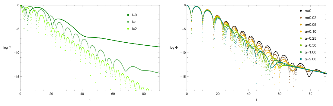
We proceed by investigating the effect of the $f(T)$ model parameter $\alpha$ , as well as of the orbital angular momentum $l$ , on the field decay behavior. Focusing on metric ansatz2, in the upper graph of Fig. 5 we present the field decay for different $l$ , varying from 0 to 2, with a massless scalar field and $\alpha$ fixed to 0.05. As we can see, for larger $l$ we have smaller period of quasinormal vibration, a behavior which is similar to the Schwarzschild case. Furthermore, in the lower graph of Fig. 5, we depict the field decay for different $\alpha$ , with fixed $l=1$ . The $\alpha=0$ curve corresponds to the Schwarzschild case, while the $\alpha\neq 0$ curves present the effect of the $f(T)$ modification. We can see that the field decay behavior changes smoothly for different $\alpha$ . Moreover, we observe that for increasing $\alpha$ we have longer period and larger slope. This may be comprehensible since under the $f(T)$ modification the metric solution has larger slope around the event horizon (see Fig. 1), and thus larger slope for the field decay.

Finally, let us compare the cases of ansatz1 and ansatz2. In Fig. 6 we depict the decay of the massless scalar field mode function in the two cases, for $\alpha=0.05$ and $l=1$ . In order to present the comparison in a more transparent way, we display both the 3D evolution, as well as the time evolution at constant radius. As we observe, the field decay for ansatz2 is similar to the standard case of Schwarzschild metric, while for ansatz1 there is no typical power-law tail. This results from the fact that in ansatz1 the metric functions $F(r)$ and $N(r)$ have different roots, and thus the effective potential acquires a non-zero value at the event horizon, making the perturbation of the scalar field not to smooth out as in the Schwarzschild case. Lastly, note that there are also some differences in the form and slope of the various curves in the lower graph, and this leads to different results for the QNM frequencies.

3.3 WKB approximation method

In order to calculate the QNM frequency semi-analytically, we can use the WKB approximation method [96, 110]. If we define $Q=\omega^{2}-V$ , then the Schr $\ddot{\text{o}}$ dinger-like equation (3.6) acquires the form

\frac{d^{2}\Psi_{l}}{dr^{*2}}+Q(r^{*})\Psi_{l}=0.

(3.23)

For a resonant normal mode of the black hole, whose response to an external perturbation is maximal, we have the boundary condition

\lim_{r^{*}\rightarrow\pm\infty}\Psi_{l}e^{i\omega r^{*}}=1.

(3.24)

This semi-analytic method has been widely used in QNM frequency estimation. Incorporating up to N order terms, the square of the frequencies can be expressed as

\omega^{2}=V\left(x_{0}\right)-i\left(n+\frac{1}{2}\right)\sqrt{2Q_{0}^{\prime\prime}}\varepsilon-i\sqrt{2Q_{0}^{\prime\prime}}\sum_{i=2}^{N}\varepsilon^{j}\Lambda_{j},

(3.25)

where $n$ is the overtone number, $\epsilon$ is a tracking parameter, $x_{0}$ is the position of the peak of the effective potential, and all the terms are calculated at $x_{0}$ . The first two correction terms are given by [96]

$\displaystyle\Lambda_{2}(n)$	$\displaystyle=\frac{1}{(2Q_{0}^{{}^{\prime\prime}})^{1/2}}\left[\frac{1}{8}\frac{V_{0}^{(4)}}{V_{0}^{(2)}}\left(\frac{1}{4}+\xi^{2}\right)-\frac{1}{288}\left[\frac{V_{0}^{(3)}}{V_{0}^{(2)}}\right]^{2}\left(7+60\xi^{2}\right)\right]$	(3.26)
$\displaystyle\Lambda_{3}(n)$	$\displaystyle=\frac{n+\frac{1}{2}}{2Q_{0}^{{}^{\prime\prime}}}\left[\frac{5}{6912}\frac{V_{0}^{(3)4}}{V_{0}^{(2)4}}\left(77+188\xi^{2}\right)-\frac{1}{384}\frac{V_{0}^{(3)2}V_{0}^{(4)}}{V_{0}^{(2)3}}\left(51+100\xi^{2}\right)\right.$
	$\displaystyle\left.+\frac{1}{2304}\frac{V_{0}^{(4)2}}{V_{0}^{(2)2}}\left(67+68\xi^{2}\right)+\frac{1}{288}\frac{V_{0}^{(3)}V_{0}^{(5)}}{V_{0}^{(2)2}}\left(19+28\xi^{2}\right)-\frac{1}{288}\frac{V_{0}^{(6)}}{V_{0}^{(2)}}\left(5+4\xi^{2}\right)\right],$	(3.27)

where $\xi=n+\frac{1}{2}$ . Higher order correction terms can be found in Refs. [74, 75].

However, the convergence of WKB series is only asymptotical, and when the order is not high enough, the results may get worse as the order increases [76, 111]. To enhance the accuracy, the Taylor expansion in (3.25) can be replaced by the Pade approximation [75]

P_{\tilde{m}}^{\tilde{n}}(\varepsilon)=\frac{\sum_{n=0}^{\tilde{n}}A_{n}\varepsilon^{n}}{\sum_{n=0}^{\tilde{m}}B_{n}\varepsilon^{n}},

(3.28)

which is known to give satisfactory results sometimes even out of the range it’s mathematically proven to converge. Existing literature about Pade approximation showed that it can greatly improve the WKB method to get better results [75, 76], especially for extremely high order Pade approximation [112, 111], which can successfully reproduce many known results of accurate numerical calculations to high decimal places [113]. In our discussion, we use $P_{6}^{6}$ approximation to improve our WKB method calculation.

In Fig. 7 we depict how the real and imaginary parts of the QNM frequency of a massless scalar field vary with respect to the model parameter $\alpha$ , for $l=1$ , in the case of the WKB approximation method. As we can see, the effect is more significant in the ansatz2 case. We mention here that although the accuracy of the WKB approximation method depends on the effective potential of the black hole, practically it is more accurate for $l>n$ modes.

Figure 7: The real and imaginary parts of the QNM frequency for a massless scalar field with respect to the model parameter

\alpha

, for

l=1

, in the case of the WKB approximation method.

Finally, for comparison, in Table 1 we summarize the results for a massless scalar field obtained using the WKB approximation method and the time-domain characteristic integration method. And in Table 2 we give the results for electromagnetic fields.

$\alpha$	$l$	ansatz1				ansatz2
$\alpha$	$l$	WKB(Re)	WKB(Im)	Int(Re)	Int(Im)	WKB(Re)	WKB(Im)	Int(Re)	Int(Im)
0.00	0	0.221	-0.210	0.196	-0.102	0.221	-0.210	0.196	-0.102
	1	0.587	-0.195	0.559	-0.209	0.586	-0.195	0.559	-0.209
	2	0.967	-0.194	0.964	-0.192	0.967	-0.194	0.964	-0.192
0.02	0	0.352	-0.177	0.189	-0.106	0.258	-0.201	0.200	-0.102
	1	0.591	-0.196	0.562	-0.216	0.590	-0.196	0.572	-0.213
	2	0.967	-0.196	0.977	-0.205	0.967	-0.196	0.973	-0.197
0.05	0	0.215	-0.213	0.190	-0.095	0.162	-0.213	0.200	-0.108
	1	0.610	-0.204	0.508	-0.234	0.600	-0.195	0.572	-0.227
	2	0.967	-0.201	0.982	-0.214	0.968	-0.199	0.969	-0.213
0.10	0	0.197	-0.231	0.197	-0.080	0.185	-0.230	0.201	-0.115
	1	0.560	-0.218	0.496	-0.182	0.578	-0.250	0.558	-0.237
	2	0.964	-0.215	0.912	-0.278	0.964	-0.215	0.963	-0.227
0.25	0	0.261	-0.216	0.210	-0.065	0.166	-0.233	0.200	-0.128
	1	0.540	-0.212	0.494	-0.152	0.543	-0.250	0.545	-0.249
	2	0.931	-0.219	0.886	-0.186	0.942	-0.249	0.955	-0.246
0.50	0	0.179	-0.184	0.221	-0.063	0.159	-0.250	0.191	-0.150
	1	0.546	-0.234	0.453	-0.170	0.525	-0.260	0.436	-0.258
	2	0.904	-0.217	0.904	-0.283	0.908	-0.262	0.921	-0.262
1.00	0	0.181	-0.166	0.225	-0.060	0.136	-0.226	0.186	-0.171
	1	0.513	-0.187	0.424	-0.123	0.494	-0.264	0.442	-0.222
	2	0.876	-0.216	0.940	-0.239	0.867	-0.272	0.879	-0.271
2.00	0	0.233	-0.137	0.235	-0.058	0.114	-0.220	0.174	-0.192
	1	0.497	-0.186	0.443	-0.102	0.460	-0.263	0.413	-0.237
	2	0.843	-0.209	0.910	-0.227	0.820	-0.277	0.839	-0.274

Table 1: Values of the quasinormal frequencies for a massless scalar field propagating in the

f(T)

black hole, for both ansatz1 and ansatz2, based on the WKB method and the characteristic integration method. The

f(T)

model parameter

\alpha

varies from 0.02 to 2.00 in units of

2M=1

, while the multipole parameter

l

acquires the values 0, 1 and 2.

$\alpha$	$l$	ansatz1				ansatz2
$\alpha$	$l$	WKB(Re)	WKB(Im)	Int(Re)	Int(Im)	WKB(Re)	WKB(Im)	Int(Re)	Int(Im)
0.00	1	0.497	-0.185	0.499	-0.188	0.497	-0.185	0.499	-0.188
	2	0.915	-0.190	0.919	-0.190	0.915	-0.190	0.919	-0.190
	3	1.314	-0.191	1.314	-0.191	1.314	-0.191	1.314	-0.191
0.02	1	0.499	-0.190	0.498	-0.199	0.498	-0.188	0.496	-0.205
	2	0.914	-0.194	0.919	-0.203	0.914	-0.193	0.928	-0.195
	3	1.311	-0.194	1.316	-0.193	1.311	-0.194	1.315	-0.192
0.05	1	0.503	-0.200	0.411	-0.185	0.500	-0.193	0.490	-0.200
	2	0.912	-0.200	0.908	-0.210	0.913	-0.198	0.920	-0.210
	3	1.307	-0.199	1.316	-0.204	1.307	-0.199	1.313	-0.203
0.10	1	0.511	-0.220	0.412	-0.159	0.491	-0.209	0.471	-0.224
	2	0.906	-0.209	0.899	-0.209	0.905	-0.210	0.908	-0.225
	3	1.299	-0.206	1.318	-0.243	1.296	-0.211	1.305	-0.218
0.25	1	0.588	-0.343	0.388	-0.146	0.439	-0.241	0.442	-0.227
	2	0.884	-0.233	0.850	-0.171	0.882	-0.243	0.880	-0.243
	3	1.274	-0.219	1.177	-0.198	1.277	-0.238	1.271	-0.239
0.50	1	0.421	-0.173	0.393	-0.144	0.418	-0.230	0.430	-0.233
	2	0.840	-0.208	0.878	-0.269	0.844	-0.253	0.844	-0.253
	3	1.234	-0.215	1.133	-0.120	1.237	-0.255	1.240	-0.254
1.00	1	0.409	-0.154	0.393	-0.141	0.390	-0.227	0.385	-0.223
	2	0.804	-0.197	0.806	-0.219	0.803	-0.260	0.805	-0.261
	3	1.190	-0.212	1.158	-0.094	1.187	-0.266	1.190	-0.265
2.00	1	0.395	-0.145	0.391	-0.129	0.359	-0.222	0.353	-0.254
	2	0.770	-0.185	0.797	-0.193	0.756	-0.262	0.762	-0.262
	3	1.140	-0.204	1.168	-0.074	1.126	-0.272	1.125	-0.272

Table 2: Values of the quasinormal frequencies for an electromagnetic field propagating in the

f(T)

black hole, for both ansatz1 and ansatz2, based on the WKB method and the characteristic integration method. The

f(T)

model parameter

\alpha

varies from 0.02 to 2.00 in units of

2M=1

, while the multipole parameter

l

acquires the values 0, 1 and 2.

4 Conclusions and discussion

In this work we have calculated the Quasinormal modes frequencies of a test massless scalar field around static black holes solutions in $f(T)$ gravity. Focusing on quadratic $f(T)$ modifications, which is a good approximation for every realistic $f(T)$ theory, we first extracted the spherically symmetric solutions using the perturbative method, imposing two ans $\ddot{\text{a}}$ tzes for the metric functions, which suitably quantify the deviation from the Schwarzschild solution. In both cases the deviation is larger near the event horizon, since the $f(T)$ modification leads to larger slope as well as to larger radial coordinate for the1 event horizon.

As a next step we extracted the effective potential, and we showed that the deviation from General Relativity mainly happens for negative values of the tortoise coordinate $r^{*}$ . In particular, for ansatz1 the effective potential acquires a non-zero asymptotic value, which results from the fact that the two metric functions $N(r)$ and $F(r)$ have different roots. On the other hand, for ansatz2 the effective potential exhibits vanishing asymptotic value, since $N(r)$ and $F(r)$ have the same root.

Finally, we calculated the QNM frequencies of the obtained solutions. Firstly, we solved the Schr $\ddot{\text{o}}$ dinger-like equation numerically using the discretization method, and then we extracted the frequency and the time evolution of the dominant mode applying the function fit method. Secondly, we performed a semi-analytical calculation by applying the WKB method with the $P_{6}^{6}$ Pade approximation. The main results were presented in various figures, and were summarized in Table 1 and Table 2. As we showed, the results for $f(T)$ gravity are different comparing to General Relativity, and in particular we obtain a different slope and period of the field decay behavior for different values of the model parameter $\alpha$ .

Concerning the accuracy of our methods, we can see that the results of the integration and WKB methods agree, however small differences appear due to the limitations of the approximation and numerical accuracy of the two methods. On one hand, the error can arise from the order choice of the WKB approximation. In principle, one can further develop the WKB method to higher orders and agree better with accurate numerical result. On the other hand, for the cases where the quasinormal ringing is very short, the extraction of frequencies with the characteristic integration method can not give satisfactory accuracy. Since in the present study we focus on the first estimate on the QNMs as well as their dynamics within f(T), we leave the higher order calculation as well as gravitational perturbations for future work.

In summary, we have shown that $f(T)$ gravity does have an effect on the QNM frequency, comparing to General Relativity. This result may be important under the light of the increasing accuracy in gravitational-wave observations from binary systems, in which the characteristic oscillation modes can provide interesting information. Hence, the whole analysis could be used as an additional tool in order to test General Relativity and examine whether torsional gravitational modifications are possible.

Acknowledgments

We are grateful to Geyu Mo, Shengfeng Yan, Zhao Li, and Rui Niu for helpful discussions. This work is supported in part by the National Key R&D Program of China (2021YFC2203100), by the NSFC (11961131007, 11653002), by the Fundamental Research Funds for Central Universities, by the CSC Innovation Talent Funds, by the CAS project for young scientists in basic research (YSBR-006), by the USTC Fellowship for International Cooperation, and by the USTC Research Funds of the Double First-Class Initiative. ENS acknowledges participation in the COST Association Action CA18108 “Quantum Gravity Phenomenology in the Multimessenger Approach (QG-MM)”. All numerics were operated on the computer clusters LINDA & JUDY in the particle cosmology group at USTC.

References

[1] A.A. Starobinsky, A New Type of Isotropic Cosmological Models Without Singularity, Phys. Lett. B 91 (1980) 99.
[2] CANTATA collaboration, Modified Gravity and Cosmology: An Update by the CANTATA Network, 2105.12582.
[3] S. Capozziello and M. De Laurentis, Extended Theories of Gravity, Phys. Rept. 509 (2011) 167 [1108.6266].
[4] A. Addazi et al., Quantum gravity phenomenology at the dawn of the multi-messenger era – A review, Prog. Part. Nucl. Phys. 103948 (2021) 2022 [2111.05659].
[5] S. Capozziello, Curvature quintessence, Int. J. Mod. Phys. D 11 (2002) 483 [gr-qc/0201033].
[6] S. Nojiri and S.D. Odintsov, Unified cosmic history in modified gravity: from F(R) theory to Lorentz non-invariant models, Phys. Rept. 505 (2011) 59 [1011.0544].
[7] S. Nojiri and S.D. Odintsov, Modified Gauss-Bonnet theory as gravitational alternative for dark energy, Phys. Lett. B 631 (2005) 1 [hep-th/0508049].
[8] A. Nicolis, R. Rattazzi and E. Trincherini, The Galileon as a local modification of gravity, Phys. Rev. D 79 (2009) 064036 [0811.2197].
[9] T. Clifton, P.G. Ferreira, A. Padilla and C. Skordis, Modified Gravity and Cosmology, Phys. Rept. 513 (2012) 1 [1106.2476].
[10] R. Aldrovandi and J.G. Pereira, Teleparallel Gravity: An Introduction, Springer (2013), 10.1007/978-94-007-5143-9.
[11] M. Krssak, R.J. van den Hoogen, J.G. Pereira, C.G. Böhmer and A.A. Coley, Teleparallel theories of gravity: illuminating a fully invariant approach, Class. Quant. Grav. 36 (2019) 183001 [1810.12932].
[12] Y.-F. Cai, S. Capozziello, M. De Laurentis and E.N. Saridakis, f(T) teleparallel gravity and cosmology, Rept. Prog. Phys. 79 (2016) 106901 [1511.07586].
[13] G.R. Bengochea and R. Ferraro, Dark torsion as the cosmic speed-up, Phys. Rev. D 79 (2009) 124019 [0812.1205].
[14] E.V. Linder, Einstein’s Other Gravity and the Acceleration of the Universe, Phys. Rev. D 81 (2010) 127301 [1005.3039].
[15] S.-H. Chen, J.B. Dent, S. Dutta and E.N. Saridakis, Cosmological perturbations in f(T) gravity, Phys. Rev. D 83 (2011) 023508 [1008.1250].
[16] S. Bahamonde, C.G. Böhmer and M. Wright, Modified teleparallel theories of gravity, Phys. Rev. D 92 (2015) 104042 [1508.05120].
[17] J. Beltrán Jiménez, L. Heisenberg and T.S. Koivisto, Teleparallel Palatini theories, JCAP 08 (2018) 039 [1803.10185].
[18] C. Li, Y. Cai, Y.-F. Cai and E.N. Saridakis, The effective field theory approach of teleparallel gravity, $f(T)$ gravity and beyond, JCAP 10 (2018) 001 [1803.09818].
[19] S. Bahamonde, K.F. Dialektopoulos and J. Levi Said, Can Horndeski Theory be recast using Teleparallel Gravity?, Phys. Rev. D 100 (2019) 064018 [1904.10791].
[20] S. Bahamonde, K.F. Dialektopoulos, C. Escamilla-Rivera, G. Farrugia, V. Gakis, M. Hendry et al., Teleparallel Gravity: From Theory to Cosmology, 2106.13793.
[21] R. Ferraro and F. Fiorini, Modified teleparallel gravity: Inflation without inflaton, Phys. Rev. D 75 (2007) 084031 [gr-qc/0610067].
[22] Y.-F. Cai, M. Khurshudyan and E.N. Saridakis, Model-independent reconstruction of $f(T)$ gravity from Gaussian Processes, Astrophys. J. 888 (2020) 62 [1907.10813].
[23] S.-F. Yan, P. Zhang, J.-W. Chen, X.-Z. Zhang, Y.-F. Cai and E.N. Saridakis, Interpreting cosmological tensions from the effective field theory of torsional gravity, Phys. Rev. D 101 (2020) 121301 [1909.06388].
[24] D. Wang and D. Mota, Can $f(T)$ gravity resolve the $H_{0}$ tension?, Phys. Rev. D 102 (2020) 063530 [2003.10095].
[25] A. Bose and S. Chakraborty, Cosmic evolution in f(T) gravity theory, Mod. Phys. Lett. A 35 (2020) 2050296 [2010.16247].
[26] X. Ren, T.H.T. Wong, Y.-F. Cai and E.N. Saridakis, Data-driven Reconstruction of the Late-time Cosmic Acceleration with f(T) Gravity, Phys. Dark Univ. 32 (2021) 100812 [2103.01260].
[27] C. Escamilla-Rivera, G.A. Rave-Franco and J.L. Said, f(T, B) Cosmography for High Redshifts, Universe 7 (2021) 441 [2110.05434].
[28] P. Wu and H.W. Yu, Observational constraints on $f(T)$ theory, Phys. Lett. B 693 (2010) 415 [1006.0674].
[29] V.F. Cardone, N. Radicella and S. Camera, Accelerating f(T) gravity models constrained by recent cosmological data, Phys. Rev. D 85 (2012) 124007 [1204.5294].
[30] S. Nesseris, S. Basilakos, E.N. Saridakis and L. Perivolaropoulos, Viable $f(T)$ models are practically indistinguishable from $\Lambda$ CDM, Phys. Rev. D 88 (2013) 103010 [1308.6142].
[31] R.C. Nunes, A. Bonilla, S. Pan and E.N. Saridakis, Observational Constraints on $f(T)$ gravity from varying fundamental constants, Eur. Phys. J. C 77 (2017) 230 [1608.01960].
[32] S. Basilakos, S. Nesseris, F.K. Anagnostopoulos and E.N. Saridakis, Updated constraints on $f(T)$ models using direct and indirect measurements of the Hubble parameter, JCAP 08 (2018) 008 [1803.09278].
[33] B. Xu, H. Yu and P. Wu, Testing Viable f(T) Models with Current Observations, Astrophys. J. 855 (2018) 89.
[34] X. Ren, S.-F. Yan, Y. Zhao, Y.-F. Cai and E.N. Saridakis, Gaussian processes and effective field theory of $f(T)$ gravity under the $H_{0}$ tension, 2203.01926.
[35] C.G. Boehmer, A. Mussa and N. Tamanini, Existence of relativistic stars in f(T) gravity, Class. Quant. Grav. 28 (2011) 245020 [1107.4455].
[36] P.A. Gonzalez, E.N. Saridakis and Y. Vasquez, Circularly symmetric solutions in three-dimensional Teleparallel, f(T) and Maxwell-f(T) gravity, JHEP 07 (2012) 053 [1110.4024].
[37] X.-h. Meng and Y.-b. Wang, Birkhoff’s theorem in the f(T) gravity, Eur. Phys. J. C 71 (2011) 1755 [1107.0629].
[38] R. Ferraro and F. Fiorini, Spherically symmetric static spacetimes in vacuum f(T) gravity, Phys. Rev. D 84 (2011) 083518 [1109.4209].
[39] C. Pfeifer and S. Schuster, Static spherically symmetric black holes in weak f(T)-gravity, Universe 7 (2021) 153 [2104.00116].
[40] T. Wang, Static Solutions with Spherical Symmetry in f(T) Theories, Phys. Rev. D 84 (2011) 024042 [1102.4410].
[41] K. Atazadeh and M. Mousavi, Vacuum spherically symmetric solutions in $f(T)$ gravity, Eur. Phys. J. C 73 (2013) 2272 [1212.3764].
[42] M.E. Rodrigues, M.J.S. Houndjo, J. Tossa, D. Momeni and R. Myrzakulov, Charged Black Holes in Generalized Teleparallel Gravity, JCAP 11 (2013) 024 [1306.2280].
[43] G.G.L. Nashed, Spherically symmetric charged-dS solution in $f(T)$ gravity theories, Phys. Rev. D 88 (2013) 104034 [1311.3131].
[44] C. Bejarano, R. Ferraro and M.J. Guzmán, Kerr geometry in f(T) gravity, Eur. Phys. J. C 75 (2015) 77 [1412.0641].
[45] G.G.L. Nashed, Spherically Symmetric Solution in (1+4)-Dimensional $f(T)$ Gravity Theories, Adv. High Energy Phys. 2014 (2014) 830109.
[46] E.L.B. Junior, M.E. Rodrigues and M.J.S. Houndjo, Regular black holes in $f(T)$ Gravity through a nonlinear electrodynamics source, JCAP 10 (2015) 060 [1503.07857].
[47] A. Das, F. Rahaman, B.K. Guha and S. Ray, Relativistic compact stars in $f(T)$ gravity admitting conformal motion, Astrophys. Space Sci. 358 (2015) 36 [1507.04959].
[48] S. Rani, A. Jawad and M.B. Amin, Charged Noncommutative Wormhole Solutions via Power-Law $f(T)$ Models, Commun. Theor. Phys. 66 (2016) 411.
[49] M.E. Rodrigues and E.L.B. Junior, Spherical Accretion of Matter by Charged Black Holes on f(T) Gravity, Astrophys. Space Sci. 363 (2018) 43 [1606.04918].
[50] Z.-F. Mai and H. Lu, Black Holes, Dark Wormholes and Solitons in f(T) Gravities, Phys. Rev. D 95 (2017) 124024 [1704.05919].
[51] K. Newton Singh, F. Rahaman and A. Banerjee, Einstein’s cluster mimicking compact star in the teleparallel equivalent of general relativity, Phys. Rev. D 100 (2019) 084023 [1909.10882].
[52] G.G.L. Nashed and S. Capozziello, Stable and self-consistent compact star models in teleparallel gravity, Eur. Phys. J. C 80 (2020) 969 [2010.06355].
[53] M.Z. Bhatti, Stability of celestial objects and adiabatic index, Eur. Phys. J. Plus 133 (2018) 431.
[54] A. Ashraf, Z. Zhang, A. Ditta and G. Mustafa, A study of anisotropic spheres in modified gravity via embedding approach, Annals Phys. 422 (2020) 168322.
[55] A. Ditta, M. Ahmad, I. Hussain and G. Mustafa, Anisotropic stellar structures in the theory of gravity with quintessence via embedding approach, Chin. Phys. C 45 (2021) 045102.
[56] S. Bahamonde, A. Golovnev, M.-J. Guzmán, J.L. Said and C. Pfeifer, Black holes in f(T,B) gravity: exact and perturbed solutions, JCAP 01 (2022) 037 [2110.04087].
[57] S. Bahamonde, L. Ducobu and C. Pfeifer, Scalarized Black Holes in Teleparallel Gravity, 2201.11445.
[58] Event Horizon Telescope collaboration, First M87 Event Horizon Telescope Results. I. The Shadow of the Supermassive Black Hole, Astrophys. J. Lett. 875 (2019) L1 [1906.11238].
[59] Event Horizon Telescope collaboration, First M87 Event Horizon Telescope Results. VI. The Shadow and Mass of the Central Black Hole, Astrophys. J. Lett. 875 (2019) L6 [1906.11243].
[60] Event Horizon Telescope collaboration, Gravitational Test Beyond the First Post-Newtonian Order with the Shadow of the M87 Black Hole, Phys. Rev. Lett. 125 (2020) 141104 [2010.01055].
[61] LIGO Scientific, Virgo collaboration, Observation of Gravitational Waves from a Binary Black Hole Merger, Phys. Rev. Lett. 116 (2016) 061102 [1602.03837].
[62] LIGO Scientific, Virgo collaboration, Tests of general relativity with GW150914, Phys. Rev. Lett. 116 (2016) 221101 [1602.03841].
[63] Y.-F. Cai, C. Li, E.N. Saridakis and L. Xue, $f(T)$ gravity after GW170817 and GRB170817A, Phys. Rev. D 97 (2018) 103513 [1801.05827].
[64] S.-F. Yan, C. Li, L. Xue, X. Ren, Y.-F. Cai, D.A. Easson et al., Testing the equivalence principle via the shadow of black holes, Phys. Rev. Res. 2 (2020) 023164 [1912.12629].
[65] C. Li, H. Zhao and Y.-F. Cai, New test on the Einstein equivalence principle through the photon ring of black holes, Phys. Rev. D 104 (2021) 064027 [2102.10888].
[66] H.-P. Nollert, TOPICAL REVIEW: Quasinormal modes: the characteristic ‘sound’ of black holes and neutron stars, Class. Quant. Grav. 16 (1999) R159.
[67] R.A. Konoplya and A. Zhidenko, Quasinormal modes of black holes: From astrophysics to string theory, Rev. Mod. Phys. 83 (2011) 793 [1102.4014].
[68] M. Isi and W.M. Farr, Analyzing black-hole ringdowns, 2107.05609.
[69] F.J. Zerilli, Effective potential for even parity Regge-Wheeler gravitational perturbation equations, Phys. Rev. Lett. 24 (1970) 737.
[70] S. Chandrasekhar and S.L. Detweiler, The quasi-normal modes of the Schwarzschild black hole, Proc. Roy. Soc. Lond. A 344 (1975) 441.
[71] K.D. Kokkotas and B.G. Schmidt, Quasinormal modes of stars and black holes, Living Rev. Rel. 2 (1999) 2 [gr-qc/9909058].
[72] E. Berti, V. Cardoso and A.O. Starinets, Quasinormal modes of black holes and black branes, Class. Quant. Grav. 26 (2009) 163001 [0905.2975].
[73] Y. Hatsuda and M. Kimura, Spectral Problems for Quasinormal Modes of Black Holes, Universe 7 (2021) 476 [2111.15197].
[74] R.A. Konoplya, Quasinormal behavior of the d-dimensional Schwarzschild black hole and higher order WKB approach, Phys. Rev. D 68 (2003) 024018 [gr-qc/0303052].
[75] J. Matyjasek and M. Opala, Quasinormal modes of black holes. The improved semianalytic approach, Phys. Rev. D 96 (2017) 024011 [1704.00361].
[76] R.A. Konoplya, A. Zhidenko and A.F. Zinhailo, Higher order WKB formula for quasinormal modes and grey-body factors: recipes for quick and accurate calculations, Class. Quant. Grav. 36 (2019) 155002 [1904.10333].
[77] O. Dreyer, B.J. Kelly, B. Krishnan, L.S. Finn, D. Garrison and R. Lopez-Aleman, Black hole spectroscopy: Testing general relativity through gravitational wave observations, Class. Quant. Grav. 21 (2004) 787 [gr-qc/0309007].
[78] E. Berti, V. Cardoso and C.M. Will, On gravitational-wave spectroscopy of massive black holes with the space interferometer LISA, Phys. Rev. D 73 (2006) 064030 [gr-qc/0512160].
[79] M. Isi, M. Giesler, W.M. Farr, M.A. Scheel and S.A. Teukolsky, Testing the no-hair theorem with GW150914, Phys. Rev. Lett. 123 (2019) 111102 [1905.00869].
[80] P.A. Cano, K. Fransen, T. Hertog and S. Maenaut, Gravitational ringing of rotating black holes in higher-derivative gravity, Phys. Rev. D 105 (2022) 024064 [2110.11378].
[81] B. Wang, C.-Y. Lin and C. Molina, Quasinormal behavior of massless scalar field perturbation in Reissner-Nordstrom anti-de Sitter spacetimes, Phys. Rev. D 70 (2004) 064025 [hep-th/0407024].
[82] J.L. Blázquez-Salcedo, C.F.B. Macedo, V. Cardoso, V. Ferrari, L. Gualtieri, F.S. Khoo et al., Perturbed black holes in Einstein-dilaton-Gauss-Bonnet gravity: Stability, ringdown, and gravitational-wave emission, Phys. Rev. D 94 (2016) 104024 [1609.01286].
[83] G. Franciolini, L. Hui, R. Penco, L. Santoni and E. Trincherini, Effective Field Theory of Black Hole Quasinormal Modes in Scalar-Tensor Theories, JHEP 02 (2019) 127 [1810.07706].
[84] R. Bécar, P.A. González, E. Papantonopoulos and Y. Vásquez, Quasinormal modes of three-dimensional rotating Ho $\check{r}$ ava AdS black hole and the approach to thermal equilibrium, Eur. Phys. J. C 80 (2020) 600 [1906.06654].
[85] A. Aragón, P.A. González, E. Papantonopoulos and Y. Vásquez, Quasinormal modes and their anomalous behavior for black holes in $f(R)$ gravity, Eur. Phys. J. C 81 (2021) 407 [2005.11179].
[86] H. Liu, P. Liu, Y. Liu, B. Wang and J.-P. Wu, Echoes from phantom wormholes, Phys. Rev. D 103 (2021) 024006 [2007.09078].
[87] T. Karakasis, E. Papantonopoulos and C. Vlachos, f(R) gravity wormholes sourced by a phantom scalar field, Phys. Rev. D 105 (2022) 024006 [2107.09713].
[88] P.A. González, E. Papantonopoulos, J. Saavedra and Y. Vásquez, Quasinormal modes for massive charged scalar fields in Reissner-Nordström dS black holes: anomalous decay rate, 2204.01570.
[89] A. Ishibashi and H. Kodama, Stability of higher dimensional Schwarzschild black holes, Prog. Theor. Phys. 110 (2003) 901 [hep-th/0305185].
[90] A. Chowdhury, S. Devi and S. Chakrabarti, Naked singularity in 4D Einstein-Gauss-Bonnet novel gravity: Echoes and (in)-stability, 2202.13698.
[91] Y.-F. Cai, G. Cheng, J. Liu, M. Wang and H. Zhang, Features and stability analysis of non-Schwarzschild black hole in quadratic gravity, JHEP 01 (2016) 108 [1508.04776].
[92] V. Cardoso, M. Kimura, A. Maselli, E. Berti, C.F.B. Macedo and R. McManus, Parametrized black hole quasinormal ringdown: Decoupled equations for nonrotating black holes, Phys. Rev. D 99 (2019) 104077 [1901.01265].
[93] R. McManus, E. Berti, C.F.B. Macedo, M. Kimura, A. Maselli and V. Cardoso, Parametrized black hole quasinormal ringdown. II. Coupled equations and quadratic corrections for nonrotating black holes, Phys. Rev. D 100 (2019) 044061 [1906.05155].
[94] G. Guo, P. Wang, H. Wu and H. Yang, Quasinormal Modes of Black Holes with Multiple Photon Spheres, 2112.14133.
[95] C. Gundlach, R.H. Price and J. Pullin, Late time behavior of stellar collapse and explosions: 1. Linearized perturbations, Phys. Rev. D 49 (1994) 883 [gr-qc/9307009].
[96] S. Iyer and C.M. Will, Black Hole Normal Modes: A WKB Approach. 1. Foundations and Application of a Higher Order WKB Analysis of Potential Barrier Scattering, Phys. Rev. D 35 (1987) 3621.
[97] M. Krssak and E.N. Saridakis, The covariant formulation of f(T) gravity, Class. Quant. Grav. 33 (2016) 115009 [1510.08432].
[98] C. Will, Theory and experiment in gravitational physics (8, 1993).
[99] S. Bahamonde, J. Levi Said and M. Zubair, Solar system tests in modified teleparallel gravity, JCAP 10 (2020) 024 [2006.06750].
[100] A. DeBenedictis and S. Ilijic, Spherically symmetric vacuum in covariant $F(T)=T+\frac{\alpha}{2}T^{2}+\mathcal{O}(T^{\gamma})$ gravity theory, Phys. Rev. D 94 (2016) 124025 [1609.07465].
[101] S. Bahamonde, K. Flathmann and C. Pfeifer, Photon sphere and perihelion shift in weak $f(T)$ gravity, Phys. Rev. D 100 (2019) 084064 [1907.10858].
[102] X. Ren, Y. Zhao, E.N. Saridakis and Y.-F. Cai, Deflection angle and lensing signature of covariant f(T) gravity, JCAP 10 (2021) 062 [2105.04578].
[103] L. Iorio and E.N. Saridakis, Solar system constraints on f(T) gravity, Mon. Not. Roy. Astron. Soc. 427 (2012) 1555 [1203.5781].
[104] L. Iorio, N. Radicella and M.L. Ruggiero, Constraining f(T) gravity in the Solar System, JCAP 08 (2015) 021 [1505.06996].
[105] G. Farrugia, J. Levi Said and M.L. Ruggiero, Solar System tests in f(T) gravity, Phys. Rev. D 93 (2016) 104034 [1605.07614].
[106] Z. Chen, W. Luo, Y.-F. Cai and E.N. Saridakis, New test on general relativity and $f(T)$ torsional gravity from galaxy-galaxy weak lensing surveys, Phys. Rev. D 102 (2020) 104044 [1907.12225].
[107] R.B. Mann, S. Murk and D.R. Terno, Black holes and their horizons in semiclassical and modified theories of gravity, 2112.06515.
[108] V. Cardoso and J.P.S. Lemos, Quasinormal modes of Schwarzschild anti-de Sitter black holes: Electromagnetic and gravitational perturbations, Phys. Rev. D 64 (2001) 084017 [gr-qc/0105103].
[109] R.A. Konoplya and A. Zhidenko, Quasinormal ringing of general spherically symmetric parametrized black holes, Phys. Rev. D 105 (2022) 104032 [2201.12897].
[110] C. Molina, D. Giugno, E. Abdalla and A. Saa, Field propagation in de Sitter black holes, Phys. Rev. D 69 (2004) 104013 [gr-qc/0309079].
[111] J. Matyjasek and M. Telecka, Quasinormal modes of black holes. II. Padé summation of the higher-order WKB terms, Phys. Rev. D 100 (2019) 124006 [1908.09389].
[112] Y. Hatsuda, Quasinormal modes of black holes and Borel summation, Phys. Rev. D 101 (2020) 024008 [1906.07232].
[113] J. Matyjasek, Accurate quasinormal modes of the five-dimensional Schwarzschild-Tangherlini black holes, Phys. Rev. D 104 (2021) 084066 [2107.04815].

Quasinormal modes of black holes in 𝒇⁡(𝑻)f(T) gravity

Abstract

1 Introduction

2 Black holes in f⁡(T)f(T) gravity

2.1 f⁡(T)f(T) gravity

2.2 Spherically symmetric solutions

2.2.1 Ansatz 1

2.2.2 Ansatz 2

3 Quasinormal modes analysis

3.1 Schro¨\ddot{\text{o}}dinger-like equation and effective potential

3.2 Characteristic integration method

3.3 WKB approximation method

4 Conclusions and discussion

Acknowledgments

References

Quasinormal modes of black holes in $f(T)$ gravity

2 Black holes in $f(T)$ gravity

2.1 $f(T)$ gravity

3.1 Schr $\ddot{\text{o}}$ dinger-like equation and effective potential