On light surfaces in black hole thermodynamics Journal: Eur. Phys. J. C

In this section, we build the framework for the BH thermodynamics laws by using the properties of special light surfaces and the BH horizons.

BH horizons

Let us introduce the Killing vector $\mathcal{L}=\partial_{t}+\omega\partial_{\phi}$. We will consider mainly $\omega=$constant. The quantity $\mathbf{\mathcal{L_{N}}}\equiv\mathcal{L}\cdot\mathbf{\mathcal{L}}$ becomes null for photon-like particles with orbital frequencies $\omega_{\pm}$.

The Killing vector $\mathcal{L}_{\pm}\equiv\xi_{t}+\omega_{\pm}\xi_{\phi}$, where $\omega_{\pm}$ satisfy the null condition on the norm of $\mathcal{L}$, can be interpreted as generator of null curves ($g_{\alpha\beta}\mathcal{L}^{\alpha}_{\pm}\mathcal{L}^{\beta}_{\pm}=0$) as the Killing vectors $\mathcal{L}_{\pm}$ are also generators of Killing event horizons.

The Kerr horizons are null (lightlike) hypersurfaces generated by the flow of a Killing vector, whose null generators coincide with the orbits of a one-parameter group of isometries, i.e., in general, there exists a Killing field $\mathcal{L}$, which is normal to the null surface. More precisely, the BH horizon $r_{+}$ is a non-degenerate (bifurcate) Killing horizon generated by the vector field $\mathcal{L}$. In the case $a=0$ (where $\omega=0$), $\xi_{t}$ (now generator of $r_{+}$) is hypersurface-orthogonal.

Thus, the null frequencies $\omega_{\pm}$ evaluated on the BH horizons, are the BH inner and outer horizons frequencies $\omega_{H}^{\mp}$ respectively.

Light surfaces and characteristic frequencies

The results we discuss in this work follow from the investigation of the properties of the null vector $\mathcal{L}$. The framework of BH thermodynamics is constructed upon the solutions $\mathcal{MB}:\mathbf{\mathcal{L_{N}}}=0$, with $\omega=$constant, where $\mathcal{MB}$ is a spin parameter of the set $\mathcal{MB}\in\{a,a\sqrt{\sigma}\}$. Solutions $\mathcal{MB}$ are functions of $(\omega,r)$, or $(\omega,r,\sigma)$, and can be represented as a curve called metric bundle $\mathcal{MB}$ on a plane $a-r$ or $\mathcal{A}-r$ (extended plane) where $\mathcal{A}\equiv a\sqrt{\sigma}$–remnants; bundle-EPJC-complete; LQG-paper; bundle-ragtime; bundle-MG; Pugliese:2021aeb; GRG-lette.

The quantity $\omega:\mathbf{\mathcal{L_{N}}}=0$, for the null vector $\mathcal{L}$ will be called characteristic $\mathcal{MB}$ frequency.

A particular null vector $\mathcal{L}$ is defined by $\omega=\omega(r_{\pm})\equiv\omega_{H}^{\pm}$, defining the Killing horizons of the metric. In fact, the event horizons of a spinning BH are Killing horizons with respect to the Killing field $\mathcal{L}_{H}=\partial_{t}+\omega_{H}^{\pm}\partial_{\phi}$, where $\omega_{H}^{\pm}$ is the angular velocity (frequency) of the horizons representing the BH rigid rotation. The event horizon of a stationary asymptotically flat solution with matter, satisfying suitable hyperbolic equations, is a Killing horizon. The strong rigidity theorem connects the event horizon with a Killing horizon. In the limiting case of spherically symmetric, static spacetimes, the event horizons are Killing horizons with respect to the Killing vector $\partial_{t}$ and the event, apparent, and Killing horizons with respect to the Killing field $\xi_{t}$ coincide (we can say that $\omega_{H}^{+}=0)$.

Therefore, in the extended plane, the curve $a_{\pm}\equiv\sqrt{r(2M-r)}$, is called horizon curve and it is tangent at any point to a $\mathcal{MB}$ curve. The tangent point $(a_{g},r_{g})$, distinguishes the BH rotation $a_{g}$ and its outer (inner) horizon $r_{g}\in[M,2M]$ ($r_{g}\in]0,M]$). The tangent point defines the BH outer (inner) horizon frequency which, therefore, is the $\mathcal{MB}$ characteristic frequency. In the extended plane, $\mathcal{MB}$ are made by points $(a,r)$ or ($a\sqrt{\sigma},r)$ distinguishing a geometry $a$ (which can be also a naked singularity) and an orbit (and plane $\sigma$) where there is light-like frequency $\omega$ corresponding to the $\mathcal{MB}$ characteristic frequency.

Two important properties follow: all metric bundles are tangent to the horizon curves and the horizon curves are the envelope surfaces of the metric bundles. Thus, all the $\mathcal{MB}$ characteristic frequencies, all the light surfaces frequencies (also in the naked singularity solutions) are frequencies of a BH (inner or outer) horizons, determined by the corresponding $\mathcal{MB}$ tangent point. The point $a_{0}$ ($\mathcal{A}_{0}$) at the origin $r=0$ (central singularity) is called the bundle origin.

Note that in this case we are assuming $\omega>0$ as $a>0$; however, the study of counter-rotating photon circular orbits with frequency $\omega<0$ is possible with $\mathcal{MB}$s in the extended plane $a\in R$ with $\omega>0$, although in this analysis this extension is not necessary–see bundle-EPJC-complete. The NS light surfaces properties are defined by the BH light surfaces (through the condition of tangency of the bundles with the horizon curve). Vice versa it has been shown that most bundles $\mathcal{MB}$ with NS origin are tangent to the inner horizons curve. The horizon curves point $a=0,r=0$ is the central singularity, $(a=M,r=M)$ is the horizon of the extreme Kerr BH, while $a=0$ with point $r=2M$ is the horizon of the Schwarzschild solution.

Each line $a_{\pm}=$constant in this extended plane is a BH geometry, where the inner horizons are for $r\in[0,M]$ on the line $a_{\pm}$, while $r\in[M,2M]$ contains the outer horizons. The maximum of the curve $a_{\pm}$ is the point $a=M$ and $r=M$ which is the horizon in the extreme Kerr BH. The Schwarzschild BH is for $a=0$; therefore, it corresponds to the zeros of the metric bundles curves, where $r=2M$ is its horizon–and in the extended plane it coincides also with the outer ergosurface on the equatorial plane of all the Kerr BHs and NSs⁴⁴ 4 $\mathcal{MB}$s are a conformal invariants of the metric as many other quantities considered in this analysis that inherit some of the properties of the Killing vector $\mathcal{L}$.

The characteristic frequency $\omega$, the bundles origin $a_{0}$, the tangent spin $a_{g}$ and radius $r_{g}$ to the horizon curve in the extended plane are related by the following conditions

where $r_{g}\in[0,2M]$, $a_{0}\in[0,+\infty[$, $a_{g}\in[0,M]$ (with the extension to negative values for the counter-rotating case), $\omega\in[0,+\infty]$ and $\sigma\in[0,1]$.

The bundle is tangent to the horizon curve at one point only; therefore, this defines uniquely the BH with the characteristic frequency $\omega$ and, consequently, bundles can contain either only BHs or BHs and NSs. Bundles are not defined in the region $]r_{-},r_{+}[$ of BH spacetimes, but they are defined in the region $r\in[0,2M]$ of NSs).

$\mathcal{MB}$ curves in the extended plane connect points of different (BH or BH and NS) geometries having all the same characteristic null frequency $\omega$. They are related to the light surface $r_{s}(\omega):\mathcal{L}_{\mathcal{N}}=0$ defined in a fixed spacetime as the light surfaces $r_{s}$ are the collections of all points, crossing of the $\mathcal{MB}$ with a line $a=$constant on the extended plane.

Constrains on matter distribution

$\mathcal{MB}$s, defined by light-surfaces, determine also the timelike (matter circular) motion providing the limiting orbital frequencies of stationary observers.

As the solutions $\omega:\mathcal{L}_{N}=0$, for each point $(a,r,\theta)$, are generally two frequencies $\omega_{\pm}$, this implies that there are two bundles crossing at any point of the extended plane. The frequencies $\omega_{\pm}$, at the crossing point $r$, bound the possible stationary observers frequencies. Specifically, the causal structure defined by timelike stationary observers is characterized by a frequency bounded in the range $\omega\in]\omega_{-},\omega_{+}[$. On the other hand, static observers are defined by the limiting condition $\omega=0$ and cannot exist in the ergoregion.

The limiting frequencies $\omega_{\pm}$, which are photon orbital frequencies, solutions of the condition $\mathcal{L_{N}}=0$, determine the frequencies $\omega_{H}^{\pm}$ of the Killing horizons as well as the bundles characteristic frequencies.

The vector $\mathcal{L}$ appears in the description of certain BH evolution processes because it enters the definitions of thermodynamic variables and stationary observers. The vector $\mathcal{L}$, the condition $\mathcal{L_{N}}=0$ and $\mathcal{MB}$s are closely related to the definition of stationary observes, i. e., observers with a tangent vector which is a Killing vector, that is, whose four-velocity $u^{\alpha}$ is a linear combination of the two Killing vectors $\xi_{\phi}$ and $\xi_{t}$; therefore, $u^{\alpha}=\gamma\mathcal{L}^{\alpha}=\gamma(\xi_{t}^{\alpha}+\omega\xi_{\phi}^{\alpha}$), where $\gamma$ is a normalization factor and $d\phi/{dt}={u^{\phi}}/{u^{t}}\equiv\omega$. The dimensionless quantity $\omega$ is the orbital frequency of the stationary observer.

It is clear that $\mathcal{MB}$s relate different geometries through their light surfaces defined by the characteristic frequencies which are BHs frequency. Thus, they are particularly adapted to describe BH state transitions, constrained by the properties of the null vector $\mathcal{L}$, which builds up many of the thermodynamic properties of BHs. In the next section, we shall detail the BH thermodynamic properties in terms of the null vector $\mathcal{L}$ and, therefore, of the metric bundles.

$\mathcal{MB}$s are structures that are related to the points of the light surfaces of different geometries and, therefore, provide relations between geometries. This different way of rewriting the properties of the null vector $\mathcal{L}$, which defines also the BH horizons, emphasizes some geometric characteristics and properties, repeating in the same spacetime or different geometries of a $\mathcal{MB}$. One of these properties, from the light surfaces and $\mathcal{MB}$definitions is the frequency $\omega$, all the points of a $\mathcal{MB}$curve are the replica of the BH horizon frequency $\omega_{H}^{+}$ or $\omega_{H}^{-}$ of the BH individuated by the tangent point $(a_{g},r_{g})$. In some cases, these horizons (frequencies) replicas are in the same spacetime. In Pugliese:2021aeb; GRG-lette, the BH poles $\sigma\approx 0$ have been studied for the observation of the photon orbits with $\mathcal{MB}$s characteristic frequency. These are light-like (circular) orbits having the same frequency as the black hole $\omega_{H}^{\pm}$.

In the context of replicas, we also introduce the concept of horizon confinement. Indeed, we say that there is a replica when in the spacetime it is possible to find at least a couple of points having the same value for the property $\mathcal{Q}$. Then, we say that there is a confinement, when that value is not replicated. In the Kerr spacetime, part of the inner horizon frequencies are "confined". The confinement analysis, which is the study of the topology of the curves ${\omega}=$constant in the extended plane, provides information about the local properties of the spacetime replicated in regions more accessible to observes; for example, in the case of properties defined in the proximity of the BH poles or of the inner horizons. An observer can register the presence of a replica at the point $p$ of the BH spacetime with spin $a_{p}$, belonging to a Killing bundle. The observer will find the replica of the BH horizon frequency $\omega_{H}^{+}(a_{p})$ at the point $p$; therefore, her/his orbital stationary frequency is $\omega_{p}\in]\omega_{\bullet},\omega_{\star}[$ where one of ($\omega_{\bullet},\omega_{\star}$) is the horizon’s frequency $\omega_{H}^{+}$, replicated on a pair of orbits $(r_{+},r_{p})$. The second light-like frequency $\omega_{\bullet}$ is the frequency of a horizon in a BH spacetime. The relation between the two frequencies $(\omega_{\star},\omega_{\bullet})$ is determined by a characteristic ratio, which we also study Pugliese:2021aeb; GRG-lette. In general, we use in this work replicas to connect BH spacetimes related in a transition and governed by the thermodynamic laws in the extended plane. We reformulate BH thermodynamics on the replicas in terms of the light surfaces, exploring the thermodynamic properties of the geometries defined by the metric bundles.

Here we explore BH thermodynamics in the extended plane in terms of the light surfaces using $\mathcal{MB}$ curves and discuss variations of the total mass $M$, area $A_{area}$, and momentum $J$ of the BH defined by the tangency property with the horizons curve in the extended plane, considering the bundle frequency $\omega$ and the acceleration $\ell$. We emphasize some ("conformal") properties, as defined below, in these relations.

We will connect the BHs states before and after a transition by expressing their characteristics and parameters through the $\mathcal{MB}$s (curves defined by the properties of the light surfaces for different geometries) and their representation in the extended plane. Particularly the condition of tangency with the curve of the horizons provides the constraint for BHs transformations. Although the extended plane represents also NSs solutions as the origin of the bundles and the $\mathcal{MB}$s contain BHs and BHs and NSs (related to the tangency to the curve portion of the internal horizons) or depending on the $\sigma$ angle (near the poles there are interesting properties of the $\omega$ frequencies explored in Pugliese:2021aeb; GRG-lette), these transformations seem to confirm cut off of any BH-NS transition.

The problem of writing the relation between main BH quantities before and after a transition (on the horizon curve) can be rephrased as the problem of finding replicas in the extended plane. More precisely, let us consider two points, $r$ and $r_{p}$, along the horizon curve $a_{\pm}>0$, which can also be in the entire range $r\in[0,2M]$. We relate the parameters $\mathcal{P}_{\pm}=(\ell^{\pm},\omega^{\pm}_{H})$, regulating the BH transition, as evaluated on the point $r$ and $r_{p}$.

We search for a quantity $\kappa$ such that $\mathcal{P}_{\pm}(r)=\kappa\mathcal{P}^{*}_{\pm}(r_{p})$ (conformal property). Note that it can also be $\ell^{\pm}$ or $\pm\ell^{\pm}$, connecting, therefore, properties defined on an outer horizon with properties defined on an inner horizon; for this reason the notation $(*)$ represents a change in sign in one or more components of the couple. While the frequency $\omega$ is always positive (according to the sign of $J$), the surface gravity $\ell$ can be negative, when evaluated on a point of the inner horizon; therefore, it can be $\ell_{H}^{\pm}(r_{p})=\ell_{H}^{-}<0$.

We also investigate the case $\delta A_{area}^{+}=-\delta A_{area}^{-}$ occurring for $\delta M=0$ (as $\delta M^{+}=\delta M^{-}$). In here we use notation $(\pm)$ to indicate quantities evaluated on the horizons $r_{\pm}$. Moreover, $\delta\mathcal{Q}\equiv\mathcal{Q}(1)-\mathcal{Q}(0)$ denotes the change of the quantity $\mathcal{Q}$ from the initial $(0)$ to the final state $(1)$ of the transition. The point $a=M$ and $r=r_{p}=M$ corresponds to the extreme Kerr BH, where $\omega(r_{p})\neq\omega(r)$ for points $(r,r_{p})$ of the horizon curve. For the surface gravity the situation is different. There can be replicas on the curve of the horizons, which depend on $a$ and $r$ and connect inner and outer horizons; this is clearly illustrated in Figs (2).

For convenience, we report here some relations for the frequencies:

In the first equation of  (3), the frequency is defined as a function of a general point $r\in a_{\pm}$ of the inner horizon for $r\in[0,M]$ or the outer horizon for $r\in[M,2M]$. In the second expression, we explicit the inner and outer horizon frequencies.

When calculated on the inner horizon curve in the extended plane, the surface gravity reads

In first expression of Eq. (4), we denote with $\ell_{H}^{\pm}$ the acceleration for the inner horizon $\ell_{H}^{-}$ and outer horizon $\ell_{H}^{+}$ as functions of the spin $a$ or as functions of the radius $r$ on the horizon curve. The second function, instead, is the acceleration defined as function of a general point $r\in a_{\pm}$. We introduce the quantities $\ell^{-}_{+}(r)\equiv\ell_{H}^{-}(r)/\ell_{H}^{+}(r)$ and $\omega^{-}_{+}(r)\equiv\omega_{H}^{-}(r)/\omega_{H}^{+}(r)$. Using the relation $\ell_{+}^{-}(r)=-\omega_{+}^{-}(r)$, we obtain

-see Fig. (1).

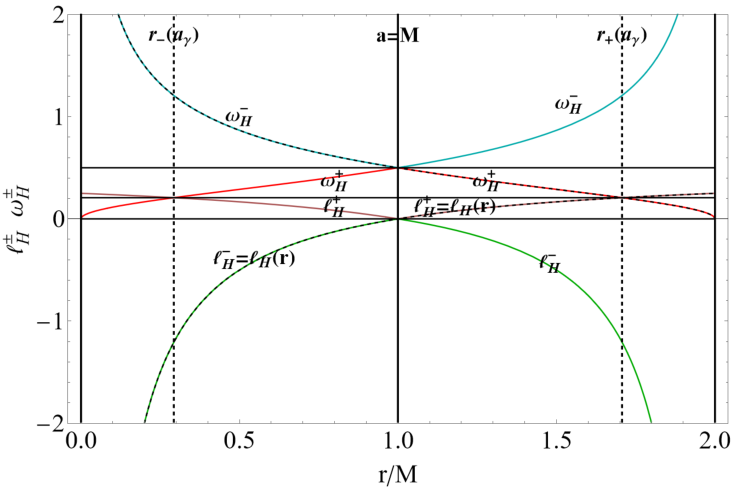
There is $\ell_{H}^{\pm}=\pm\omega_{H}^{\pm}$ for $a=a_{\gamma}\equiv 1/\sqrt{2}$.

An analogue relation holds for the quantities evaluated as functions of the spin $a$. Considering the dependence from the spin $a$ we find,

alternatively to Eq. (4). Defining $\ell_{-}^{+}(a)\equiv\ell_{H}^{+}(a)/\ell_{H}^{-}(a)$ and $\omega_{-}^{+}(a)\equiv\omega_{H}^{+}(a)/\omega_{H}^{-}(a)$, we obtain $\omega_{-}^{+}(a)=-\ell_{-}^{+}(a)$ and

see also Eq. (5) and Figs (2).

Here, we search for the relation $\delta M(a_{p})^{\star}=s\delta M(a)^{\ast}$, where $a\in[0,M]$ and $a_{p}\in[0,M]$ are two BH geometries. For the particular case $a=a_{p}$, the couple $(\star,\ast)$ denotes that $\star$ or $\ast$ are $\pm$, relating to the inner-inner horizons of the two geometries or outer-outer or inner-outer horizons of the two geometries $(a,a_{p})$. The special case $a=a_{p}$ contains $(\star=\ast=\pm,s=1)$. The case considered for the quantities as functions of $r$, where $\star=-\ast=\pm$ and $s$, satisfies conditions (5). The apparent contradiction in this case is that for a fixed spacetime $a\in\textbf{BH}$, we have that $\delta M^{+}=\delta M^{-}$, but the relation regulating this variation with the other characteristic quantities depends on the point as $\delta M^{+}=s\delta M^{-}$ (where we have used the notation $\pm$ to stress quantities in relations evaluated on the horizons $r_{\pm}$, respectively).

Then, we obtain

We note also the coincidence $\omega_{H}^{\pm}(r)=\ell_{H}^{\pm}(r)=\mathcal{Q}_{\ell\omega}^{+}\equiv{1}/{\sqrt{2}}-{1}/{2}$ in the form of Eq. (3) and Eq. (4) for $r=r_{+}=\left(\sqrt{2}+2\right)/2$. This is the outer horizon for the BH geometry with spin $a/M=a_{\gamma}=1/\sqrt{2}$, specifically, $\ell_{H}^{\pm}=\pm\omega_{H}^{\pm}$. Therefore, for this spacetime the mass variation has a special for when written in the extended plane $\delta M^{\pm}=\mathcal{Q}_{\ell\omega}^{\pm}\delta\tilde{M}^{\pm}$ (where $\delta\tilde{M}^{\pm}\equiv\pm\delta A^{\pm}_{area}+\delta J^{\pm})$, where $\mathcal{Q}_{\ell\omega}^{-}=\omega_{H}^{-}={1}/{2}+{1}/{\sqrt{2}}=-\ell_{H}^{-}$.

We analyze the more general problem addressing firstly the special case $s=1$ and secondly the general case with $s\neq 1$.

The case $s=1$

This problem can be reduced to finding replicas for $\ell\left(r_{+}(a_{p})\right)=-\ell\left(r_{-}(a)\right)$, solved for

$\displaystyle\frac{2\sqrt{2}}{3}<a\leq 1,\quad a_{p}=a^{y}_{p}\equiv\frac{\sqrt{4\left(1-a^{2}\right)^{3/2}+12a^{4}-15a^{2}+4}}{4a^{2}-3}$

(10)

– Figs (2). The cases $\ell\left(r_{\pm}(a_{p})\right)=-\ell\left(r_{\pm}(a)\right)$ are solved for $a=a_{p}=M$, while $\ell_{H}^{\pm}(a)=\ell_{H}^{\pm}(a_{p})$ for $a=a_{p}$. The case $a/M=\sqrt{{8}/{9}}$ implies $(\ell_{H}^{-}=-1/4,\ell_{H}^{+}=1/8)$ and $\omega_{H}^{-}={1}/{\sqrt{2}},\omega_{H}^{+}={1}/{2\sqrt{2}}$. Therefore $(\ell_{H}^{-},\omega_{H}^{-})-=2(-\ell_{H}^{+},\omega_{H}^{+})$.

The case $s\neq 1$.

As seen for the BH spin $a/M=\sqrt{{8}/{9}}$, now we extend the problem of finding replicas by searching for orbits that relate the surface gravity and frequency as follows

$\displaystyle\omega_{H}(r_{p})=s\omega_{H}(r)\quad{and}\quad\ell_{H}(r_{p})=-s\ell_{H}(r)$

(11)

for $s\geq 0$ (the situation for $s<0$, implying a change of the BH spin rotation, provides a result analogue to the case $s>0$) that is a conformal transformation from an outer horizon $r_{+}$ to an inner horizon $r_{-}=r$. We obtain:

$\displaystyle r=\frac{2s}{s+1}\quad\mbox{ and}\quad r_{p}\equiv\frac{2}{s+1},$

(12)

therefore, $r/r_{p}=s$, and the conformal relation can be also expressed as

$\displaystyle\omega_{H}(r_{p})=(r/r_{p})\omega_{H}(r)\;and\;-\ell_{H}(r_{p})=(r/r_{p})\ell_{H}(r).$

(13)

The frequencies and accelerations are

	$\displaystyle\omega(r)=\frac{1}{2\sqrt{s}},\quad\omega(r_{p})=\frac{\sqrt{s}}{2},$		(14)
	$\displaystyle\ell(r)=\frac{s-1}{4s},\quad\ell(r_{p})=\frac{1-s}{4}$

then

	$\displaystyle\left(\omega(r_{p}),\ell(r_{p})\right)=s\left(\omega(r),-\ell(r)\right),\quad\mbox{where}\quad\frac{r}{r_{p}}=s$		(15)
	$\displaystyle\mbox{with}\quad a(r)=a(r_{p})=2\sqrt{\frac{s}{(s+1)^{2}}}=\sqrt{rr_{p}}=\sqrt{s}r_{p}$

The radii $r$ and $r_{p}$ correspond to the horizons of the BH spacetime with $a(r)=a(r_{p})$. It is clear that $(r,r_{p})$ represent a horizon parametrization and $a(r_{p})$ can be seen as analogue to the tangent curve of the horizon $a_{g}(\omega)$, function of the frequency $\omega$. It is clear from Eqs (12) and (14) that there are two ranges, $s<1$ and $s>1$, describing the same spacetime (horizontal line in the plot of $a(r_{p})=a(r)$ as function of $s$). For $s<1$, we have that $r=r_{-}$ and $r_{p}=r_{+}$ while for $s>1$, we obtain $r=r_{+}$ and $r_{p}=r_{-}$. The limiting case $s=1$ corresponds to the extreme Kerr BH.

Therefore, Eqs (11) hold for two points $(r,r_{p})$ only, the horizons of a BH spacetime with $a=a(r_{p})$. There are two values of $s=\bar{s}>1$ and $s=1/\bar{s}<1$ for the same spacetime. The remarkable aspect of this relation is that the conformal factor is different according with the spin $\hat{s}_{\mp}\equiv[({2-a^{2}})\mp 2\sqrt{({1-a^{2}})}]/{a^{2}}$, see Figs (3).

In Sec. (5.1), we will study these relations in detail.

The horizon surface area (on the event horizon $r_{+}$) is $A_{area}=16\pi M_{irr}^{2}$ and determines the BH irreducible (or rest) mass $M_{irr}=\sqrt{a^{2}+r_{+}^{2}}/2$.

The total BH mass $M$ of the Kerr BH can be decomposed into the mass $M_{irr}$ and the rotational energy.

From the first law of BH thermodynamics, we obtain $M^{2}=M_{irr}^{2}+J^{2}/4M_{irr}^{2}$, where $J$ is the BH angular momentum in units of mass $M$, as measured in the asymptotical flat region.

The maximum rotational energy which can be extracted from the black hole is $\xi\propto(M-M_{irr})$. A result of Christodolou and Ruffini sets an upper limit on the amount of energy that can be extracted from a Kerr BH as the total rotational energy, assuming a Schwarzschild BH as the final state, and the the bottom limit⁷⁷ 7 The upper limit for the energy extraction from a stationary process bringing the BH to the state $(1)$ is $M(0)-M_{irr}(M(0),J(0))$, where $M(0)$ and $J(0)$ are the mass and angular momentum of the initial state and the BH angular momentum after the process, the state $(1)$, is zero– ella-correlation. of $M$ at the end of stationary process of the energy extraction, has to be $M_{irr}$.

Within these assumptions, the maximum rotational energy which can be extracted is the limit of $\xi=\xi_{\ell}\equiv\left(2-\sqrt{2}\right)/2$, hence $\xi\in[0,\xi_{\ell}]$, where at the state $(0)$ (prior to the extraction) there is an extreme Kerr spacetime (with spin $a=M$). Considering $(0)$ as the state prior the extraction, from the law $M_{irr}^{2}=r_{+}(J,M)/2$, we obtain

from the variation we find

where $\delta M_{irr}\geq 0$, thus $(\delta M-\delta J\omega_{H}(0))\geq 0$ and $\omega_{H}\equiv\omega_{H}^{+}$ is the frequency of the outer Killing horizon for the initial BH, imposing limits on the BH spin-shift⁸⁸ 8 Measuring $\xi$, therefore, will provide and indication of the BH spin. This method, independent of the specific model of energy extraction, was introduced first in Daly0, and applied in other analysis in Daly0; Daly2; Daly3; GarofaloEvans; ella-correlation. relating the dimensionless BH spin $a/M$ to the dimensionless ratio $\xi$, where $\xi$ represents the total released rotational energy versus BH mass (measured by an observer at infinity), assuming a process ending with the total extraction of the rotational energy of the central Kerr BH. . We obtain $M^{2}={J(0)^{2}}/({4M_{irr}^{2}})+M_{irr}^{2}$, and the (extracted rotational) energy is essentially

Note that here $\xi$ has units of mass, the dimensionless spin $a_{g}/M\equiv J(0)/M(0)^{2}$ refers to an initial state before the transition, defined by the mass $M(0)$ and spin $J(0)$, which is a function of the extracted rotational energy $\xi/M(0)$, that is, $1-M_{irr}(0)/M(0)$, and, therefore, of the ratio $M_{irr}(0)/M(0)$.

On the other hand, the radius $r/M$ on the extended plane can be expressed in terms of the total mass $M(0)$. We can write the dimensionless spin as $a_{g}=a_{\xi}$ as

The function $a_{\xi}(\xi)$ links the former state spin $a_{0}$ to the rotational extraction in the subsequent phase, where the BH is settled in a Schwarzschild spacetime. The function $a_{\xi}$ is, therefore, an expression for the tangent spin in the extended plane as function of the rotational energy parameter $\xi$. Here and in the following, we shall use dimensionless quantities.

Equivalently, we can express the rotational energy parameter as

Considering $a_{\xi}(\xi)\equiv a_{s}^{(\pm)}$, solving for $\xi$ there is

relating directly the energy parameter $\xi$ to the horizons. As $\xi\propto M-M_{irr}$ (here $\xi$ has units of mass $M$), only the solution $\xi_{-}^{+}$ has to be considered. The general solution $a_{\xi}(\xi)=a_{s}^{(\pm)}$, for a couple of spins $a_{s}^{(\pm)}$, provides the eight functions $\xi_{s}^{(\pm)}$. For the point $\xi=1$, it is $a_{\xi}({\xi})=0$ with $\xi=0$. There is a maximum that depends on the spin, $\xi_{\ell}\equiv\left(2-\sqrt{2}\right)/2$ (and $\xi_{m}\equiv\left(2+\sqrt{2}\right)/2$), where $a_{\xi}(\xi)=M$ and $r_{+}=M$ (the extreme Kerr BH). In general, it is $a_{\xi}(\xi)\in[0,M]$ (dimensionless) and the definition of the rotational energy as $1-M_{irr}/M$, with restricted range $\xi\in[0,\xi_{\ell}]$, where $\xi_{\ell}\equiv\left(2-\sqrt{2}\right)/2$, limiting, therefore, the energy extracted to a maximum of $\approx 29\%$ of the mass $M$. We can express the extracted energy in terms of characteristic frequency of the bundle and through the tangency condition of the bundle in the extended plane. We introduce the curves $\xi_{\tau\tau}^{\mp}$ and $\xi_{\tau}^{\mp}$ in the extension of the plane for extended values of $\xi$, considering the BH horizon frequencies $\omega_{H}^{\pm}$, the horizon curves in the plane $\xi-r/M$, and the functions $\xi_{\mu}^{\mp},\xi_{\nu}^{\mp}$ from the other two solutions of $a=a_{\xi}(\xi)$:

References

- (1) S. Hawking, Phys. Rev. Lett. 26, 1344 (1971).
- (2) S. W. Hawking, Nature 248,30-31, (1974).
- (3) S.W.Hawking, Comm. Math. Phys. 43, 199 (1975) Erratum - ibidem 46, 206 (1976).
- (4) R. Penrose, Revista del Nuovo Cimento (1969).
- (5) M. Isi, W. M. Farr, M. Giesler, et al.Phys. Rev. Lett. 127, 1, 011103 (2021).
- (6) M. Simpson& R. Penrose, Int. J. Theor. Phys. 7 (1973).
- (7) M. Dafermos & J. Luk, The interior of dynamical vacuum black holes I: The C0-stability of the Kerr Cauchy horizon, [arXiv:1710.01722 [gr-qc]]).
- (8) J. D. Bekenstein, Phys. Rev. D 7, 2333 (1973).
- (9) J.D. Bekenstein, Phys. Rev. D, 12, 3077 (1975).
- (10) J. Polchinski, Contribution to: TASI 2015, 353-397 (2016).
- (11) Z. Stuchlík et al., Class. Quantum Grav. 28 155017, (2011).
- (12) D. Pugliese& H. Quevedo, Eur. Phys. J. C 79, 3, 209 (2019).
- (13) D. Pugliese& H. Quevedo, Eur.Phys.J. C 81, 3, 258 (2021).
- (14) D. Pugliese&G. Montani, Entropy 22 , 402 (2020).
- (15) D. Pugliese& H. Quevedo, [arXiv:1910.04996 [gr-qc]] (2019).
- (16) D. Pugliese&H. Quevedo, [arXiv:1910.02808 [gr-qc]] (2019).
- (17) D. Pugliese&H. Quevedo, Nucl. Phys. B 972, 115544 (2021).
- (18) D. Pugliese& H. Quevedo, Gen Relativ Gravit 53, 89 (2021).
- (19) P. T. Chrusciel, J. Lopes Costa, M. Heusler, Living Rev. Rel. 15, 7 (2012).
- (20) R. M. Wald, Class. Quant.Grav.16, A177 (1999).
- (21) T. Jacobson and G. Kang, Class. Quantum Grav., 10 L201 (1993).
- (22) R. M. Wald, Living Rev. Relativ. 4(1), 6 (2001).
- (23) D. Pugliese& Z. Stuchlík, Class. Quant. Grav. 38, 14, 14 (2021).
- (24) R. A. Daly, APJ, 691–L72-L76, 1 (2009).
- (25) R.. A. Daly, MNRAS, 414, 1253-1262 (2011).
- (26) R. A. Daly &T. B. Sprinkle, MNRAS, 438, 3233-3242 (2014).
- (27) R. A. Daly, APJ, 691, L72 (2009).
- (28) D. Garofalo, D. A. Evans, R. M. Sambruna, MNRAS, 406, 975-986 (2010).
- (29) D. Pugliese & Z. Stuchlík, PASJ,73 6, 1497-1539 (2021).