A Generalization of Ripley’s K Function for the Detection of Spatial Clustering in Areal Data

Suppose we are observing a spatial point process on a two dimensional region $\mathscr{A}$, with density $\lambda$. For a distance $r>0$, Ripley’s $K$ function is defined as

$$K(r)=\lambda^{-1}E(\text{number of points within a distance of $r$ of any given point}).$$

If we have observed a collection of $n$ points, we can estimate Ripley’s K function as

$$\hat{K}(r)=\hat{\lambda}^{-1}\sum_{i=1}^{n}\sum_{j=1}^{n}\frac{w_{ij}}{n}$$

where $\hat{\lambda}=n/|\mathscr{A}|$, $|\mathscr{A}|$ denotes the area of $\mathscr{A}$, and $w_{ij}$ is a weight associated with points $i$ and $j$. In the traditional approach, $w_{ij}=1$ if the distance between points $i$ and $j$ is less than $r$ and 0 otherwise (Ripley 1976; Ripley 1977). However, many variants of Ripley’s K function exists which modify these weights to account for edge effects (Ripley 1976; Sterner et al. 1986; Diggle 1983; Szwagrzyk and Czerwczak 1993; Upton and Fingleton 1985; Getis and Franklin 1987; Andersen 1992). In practice, Ripley’s K function is often re-scaled to Ripley’s L function, $\hat{L}(r)=\{\hat{K}(r)/\pi\}^{1/2}$.

Ripley’s K function is often used to determine if an observed collection of points exhibits complete spatial randomness (CSR) (i.e. the points arise from a two-dimensional homogeneous Poisson process). For a homogeneous Poisson process on an infinite study area, $K(r)=\pi r^{2}$. The distribution of $\hat{K}(r)$ under CSR for a finite study area $\mathscr{A}$ can be approximated with Monte Carlo simulations, which are used to perform a hypothesis test with the null hypothesis being that the observed data arises from a homogeneous Poisson process with rate parameter $\hat{\lambda}$. Large values of $\hat{K}(r)$ indicate spatial clustering, that is, the number of points within a distance of $r$ of any given point is larger than would be expected if the data exhibited CSR. Small value of $\hat{K}(r)$ indicate dispersion, that is, the number of points within a distance of $r$ of any given point is smaller than would be expected under CSR. For an overview of Ripley’s K function, edge correction methods, and hypothesis testing via Monte Carlo simulations, see Dixon 2014.

While Ripley’s K function is designed for point process data, in practice, it is often used to assess areal data for clustering. Areal units with some binary characteristic of interest are mapped to their centroids and Ripley’s K function is applied to to the resulting set of points. The lack of suitable alternative methods to assess clustering in areal data as well as the fact that ArcGIS applies Ripley’s K to polygon centroids by default both contribute to this misuse (ESRI 2021b). Applying Ripley’s K to the centroids of areal units is particularly problematic when the units are vastly different sizes. For example, in one of our motivating data applications we wish to determine if land parcels having conservation easements (CEs) are clustered. Under the null hypothesis, all parcels are equally likely to have a CE. Under the null hypothesis, a portion of the study area with many small parcels (such as a metropolitan area), will have more parcels with CEs than portions of the study area with many large parcels, simply because there are more parcels per unit area. Put another way, centroids of smaller parcels will appear clustered relative to centroids of larger parcels simply because the size of the small parcels allows the centroids to be closer together.

To surmount these difficulties, we propose a modification to Ripley’s K function. Suppose we have a study area $\mathscr{A}$ divided into $N$ areal units $a_{1},a_{2},...,a_{N}$, and that each unit $a_{i}$ possesses some characteristic of interest with probability $p_{i}$. For each unit, we define the Bernoulli$(p_{i})$ random variable $Y_{i}$ to be 1 if unit $i$ possesses the trait of interest and 0 otherwise. For example, $\mathscr{A}$ might be a county, $a_{1}$,…$a_{N}$ be the parcels of land in the county, and $Y_{i}=1$ if parcel $i$ contains a CE. We will refer to the subset of the units for which $Y_{i}=1$ as the ‘observed units’ or the ‘observations’, and denote them by $\mathscr{B}(\boldsymbol{Y})=\{a_{i}:Y_{i}=1\}$, where $\boldsymbol{Y}=(Y_{1},...,Y_{N})^{\prime}$. For a given study area $\mathscr{A}$, set of areal units $a_{1},...,a_{N}$, and observed data $\boldsymbol{y}$, for $r>0$ and each $i$ for which $y_{i}=1$, define

$$m(r,i,\boldsymbol{y})=\frac{|c_{i}(r)\cap\mathscr{B}(\boldsymbol{y})|}{\pi r^{2}}$$

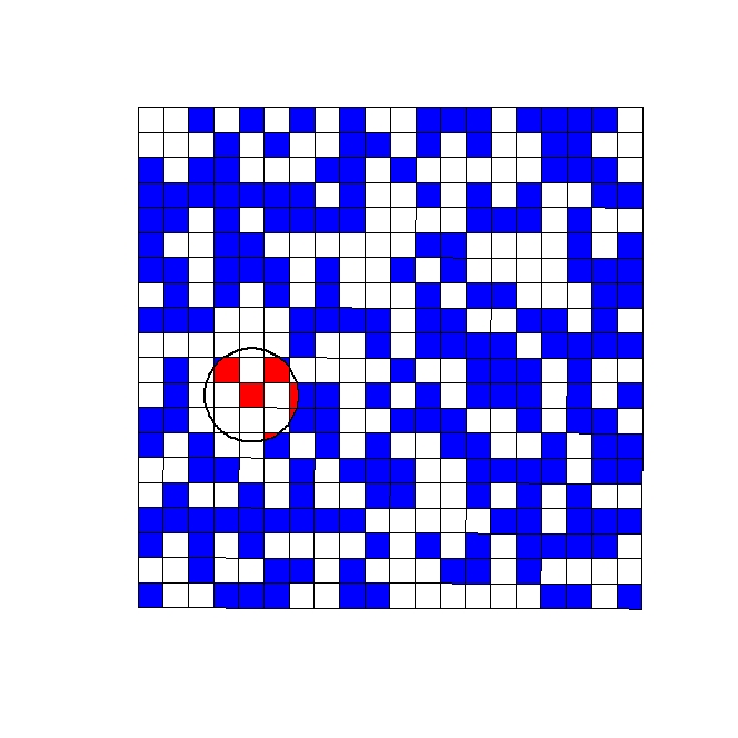
where $c_{i}(r)$ denotes the circle of radius $r$ centered at the centroid of $a_{i}$. Thus $m(r,i,\boldsymbol{y})$ is the proportion of the circle of radius $r$ centered at the centroid of $a_{i}$ which falls into the observed units (see Figure 1). Note that $m(r,i,\boldsymbol{y})$ is only defined if $a_{i}\in\mathscr{B}(\boldsymbol{Y})$. Additionally, define $m(r,\boldsymbol{y})$ as the sample average (taken over all $n_{\boldsymbol{y}}=\sum_{i=1}^{N}y_{i}$ observed units) of the amount of area within a distance of $r$ of an observed unit centroid which falls into observed units.

$$m(r,\boldsymbol{y})=\frac{1}{n_{\boldsymbol{y}}}\sum_{i:y_{i}=1}m(r,i,\boldsymbol{y}).$$

Finally, define Ripley’s K function for areal data (RKAD) by

$$m(r)=E\{m(r,\boldsymbol{Y})\}=\sum_{\boldsymbol{y}\in\mathscr{Y}}\left(\frac{1}{n_{\boldsymbol{y}}}\sum_{i:y_{i}=1}\frac{|c_{i}(r)\cap\mathscr{B}(\boldsymbol{y})|}{\pi r^{2}}\right)P(\boldsymbol{Y}=\boldsymbol{y})$$

where $\mathscr{Y}=\{(y_{1},...,y_{N}):y_{i}\in\{0,1\}\}$. Therefore,

$$m(r)=\pi^{-1}r^{-2}E(\text{observed area within a distance of $r$ of an observed unit centroid}).$$

Also define

$$m(r;n_{\boldsymbol{y}})=E\{m(r,\boldsymbol{Y})|n_{\boldsymbol{Y}}=n\}=\sum_{\boldsymbol{y}\in\mathscr{Y}_{n}}\left(\frac{1}{n}\sum_{i:y_{i}=1}\frac{|c_{i}(r)\cap\mathscr{B}(\boldsymbol{y})|}{\pi r^{2}}\right)P(\boldsymbol{Y}=\boldsymbol{y}|n_{\boldsymbol{Y}}=n)$$

where $\mathscr{Y}_{n}=\{\boldsymbol{y}\in\mathscr{Y}:\sum_{i=1}^{N}y_{i}=n\}$. Thus

	$\displaystyle m(r;n)=\pi^{-1}r^{-2}E($	observed area within a distance of $r$ of an observed unit centroid
		$\displaystyle|\text{n units were observed})$

While $m(r)$ and $m(r;n_{\boldsymbol{y}})$ may be calculated explicitly provided the vector of probabilities $\boldsymbol{p}=(p_{1},...,p_{N})^{\prime}$ is known, doing so involves computing (respectively) a $2^{N}$ and an $\binom{N}{n_{\boldsymbol{y}}}$ dimensional sum, and Monte Carlo approximations are likely to be more practical when $N$ is large.

A test for clustering or dispersion in the observed units may be derived by comparing the observed $m(r,i,\boldsymbol{y})$ values to $m(r;n_{\boldsymbol{y}})$ calculated in the absence of spatial dependence. Consider the following test statistic

$$T(r,\boldsymbol{y})=\frac{1}{n_{\boldsymbol{y}}}\sum_{i:y_{i}=1}|m(r,i,\boldsymbol{y})-m(r;n_{\boldsymbol{y}})|$$

where $m(r;n_{\boldsymbol{y}})$ is calculated under an assumed null distribution which lacks spatial dependence. Values of $T(r,\boldsymbol{y})$ which are large or small relative to the null distribution indicate a departure from the null distribution. When units exhibit clustering, certain part(s) of the study area will contain more units than expected under the null distribution. As a consequence, other parts of the study area will have fewer units than expected (as the areas in between the clusters must be sparse in comparison). Therefore values of $m(r,i,\boldsymbol{y})$ which are much larger or much smaller than $m(r;n_{\boldsymbol{y}})$ are both indicative of clustering. Consequently, a large value of $T(r,\boldsymbol{y})$ (i.e. a large average absolute difference between the observed $m(r,i,\boldsymbol{y})$’s and the estimated value $m(r,n_{\boldsymbol{y}})$ under the null distribution) indicates spatial clustering. When the areal units are dispersed, that is, distributed at more regular intervals than expected in the absence of spatial dependence, then variability in the $m(r,i,\boldsymbol{y})$’s will be decreased and the average absolute difference between the $m(r,i,\boldsymbol{y})$s and $m(r,n_{\boldsymbol{y}})$ under the null distribution will be small. Therefore, small values of $T(r,\boldsymbol{y})$ indicate dispersion.

While the sampling distribution of $T(r,\cdot)$ is not amenable to direct evaluation, it can be approximated via Monte Carlo simulations. The same Monte Carlo simulations can be used to approximate $m(r;n_{\boldsymbol{y}})$. Such an approximation involves specification of the null distribution. The class of distributions which lack spatial dependence is too broad to be practical, and the class must be narrowed in some way. As is typical for hypothesis tests for spatial dependence, we take the case of independent and identically distributed observations as our null distribution (for exact specifications, see Section 3). An approximately $\alpha$-level hypothesis test for clustering can be conducted by rejecting the null hypothesis if $T(r,\boldsymbol{y})$ exceeds the $1-\alpha$th quantile of the Monte Carlo sample of $T(r,\cdot)$. Similarly, a test for dispersion can be conducted by rejecting the null hypothesis if $T(r,\boldsymbol{y})$ is less than the $\alpha$th quantile of the Monte Carlo sample.

In this section, we perform an extensive simulation study to compare the performance of RKAD to that of the ANN method, the spatial scan statistic, and the traditional Ripley’s K function. We consider the performance of our proposed hypothesis testing procedure using two study areas which are shown in Figure 2:

	$\displaystyle\mathscr{A}_{1}:$	A 20 by 20 regular grid of $N_{1}=400$ cells
	$\displaystyle\mathscr{A}_{2}:$	The $N_{2}=3,108$ counties (and county-equivalents) in the contiguous United States

For each study area, we also consider 12 scenarios in which the locations of observed units are clustered. First, we assess the ability of our hypothesis test to detect large-scale spatial clustering which exists in only one part of the study area. We consider the following 6 scenarios:

	$C_{1}$:	$\displaystyle\boldsymbol{Y}\sim\text{SWoR}(N_{j},\lceil N_{j}/10\rceil,\boldsymbol{p}_{jC_{1}})$
	$C_{2}$:	$\displaystyle\boldsymbol{Y}\sim\text{SWoR}(N_{j},\lceil N_{j}/10\rceil,\boldsymbol{p}_{jC_{2}})$
	$C_{3}$:	$\displaystyle\boldsymbol{Y}\sim\text{SWoR}(N_{j},\lceil N_{j}/4\rceil,\boldsymbol{p}_{jC_{3}})$
	$C_{4}$:	$\displaystyle\boldsymbol{Y}\sim\text{SWoR}(N_{j},\lceil N_{j}/4\rceil,\boldsymbol{p}_{jC_{4}})$
	$C_{5}$:	$\displaystyle\boldsymbol{Y}\sim\text{SWoR}(N_{j},\lceil N_{j}/2\rceil,\boldsymbol{p}_{jC_{5}})$
	$C_{6}$:	$\displaystyle\boldsymbol{Y}\sim\text{SWoR}(N_{j},\lceil N_{j}/2\rceil,\boldsymbol{p}_{jC_{6}}).$

The $N_{j}$-dimensional vectors $\boldsymbol{p}_{jC_{l}}=(p_{jC_{l}1},\ldots,p_{jC_{l}N_{j}})^{\prime}$, $j=1,2$, $l=1,...,6$ are defined as follows: an entry of $p_{jC_{l}}$ is equal to $q/D$ if the unit is shown in blue in Figure 3 and equal to $1/D$ otherwise where $D$ is such that $\sum_{i}p_{jC_{l}i}=1$. For $C_{1}$, $C_{3}$ and $C_{5}$, we take $q=5$ and for $C_{2}$, $C_{4}$ and $C_{6}$ we take $q=10$. Thus the blue units are 5 times more likely to be observed than the white units under data generation mechanisms $C_{1}$, $C_{3}$ and $C_{5}$ and 10 times more likely to be observed under data generation mechanisms $C_{2}$, $C_{4}$ and $C_{6}$.

Next, we assess the ability of our hypothesis test to detect spatial clustering at a smaller scale when it occurs at multiple clusters spread through the study area by considering the following 6 scenarios:

	$C_{7}$:	$\displaystyle\boldsymbol{Y}\sim C(\lceil N_{j}/10\rceil,\lceil N_{j}/100\rceil,5)$
	$C_{8}$:	$\displaystyle\boldsymbol{Y}\sim C(\lceil N_{j}/10\rceil,\lceil N_{j}/100\rceil,10)$
	$C_{9}$:	$\displaystyle\boldsymbol{Y}\sim C(\lceil N_{j}/4\rceil,\lceil N_{j}/40\rceil,5)$
	$C_{10}$:	$\displaystyle\boldsymbol{Y}\sim C(\lceil N_{j}/4\rceil,\lceil N_{j}/40\rceil,10)$
	$C_{11}$:	$\displaystyle\boldsymbol{Y}\sim C(\lceil N_{j}/2\rceil,\lceil N_{j}/20\rceil,5)$
	$C_{12}$:	$\displaystyle\boldsymbol{Y}\sim C(\lceil N_{j}/2\rceil,\lceil N_{j}/20\rceil,10)$

Here, $\boldsymbol{Y}\sim C(k,m,q)$ denotes that $\boldsymbol{Y}$ is generated as follows. First, $m$ elements of $\{1,2,...,N\}$ are randomly selected via SWoR$(N_{j},m,p_{jI})$. Next, $k-m$ elements of $\{1,2,...,N\}$ are selected via SWoR$(N,k-m,\boldsymbol{p}_{2})$, where $p_{2i}=0$ if $i$ was one of the first $m$ elements selected, $p_{2i}=q/D$ for $i$ such that $a_{i}$ shares a border with at least one of the initially selected $k$ elements (but $i$ itself was not initially selected) and $p_{2i}=1/D$ otherwise, where $D$ is chosen so that $\sum_{i}p_{2i}=1$; $\boldsymbol{Y}_{i}=1$ if element $i$ was selected in either the first or second step, and $\boldsymbol{Y}_{i}=0$ otherwise, and areal unit $a_{i}$ is observed if and only $Y_{i}=1$. Note that data generation mechanisms $C_{7}$, $C_{9}$ and $C_{11}$ correspond to ‘weaker’ clustering, in the sense that they tend to select fewer adjacent units than mechanisms $C_{8}$, $C_{10}$ and $C_{12}$

Finally, we assess the ability of our hypothesis testing procedure to detect spatial dispersion under the following 4 scenarios.

	$D_{1}$:	$\displaystyle\boldsymbol{Y}\sim C\left(\lceil N_{j}/10\rceil,\lceil N_{j}/100\rceil,\frac{1}{10}\right)$
	$D_{2}$:	$\displaystyle\boldsymbol{Y}\sim C\left(\lceil N_{j}/10\rceil,\lceil N_{j}/100\rceil,0\right)$
	$D_{3}$:	$\displaystyle\boldsymbol{Y}\sim C\left(\lceil N_{j}/6\rceil,\lceil N_{j}/100\rceil,\frac{1}{10}\right)$
	$D_{4}$:	$\displaystyle\boldsymbol{Y}\sim C\left(\lceil N_{j}/6\rceil,\lceil N_{j}/100\rceil,0\right)$

Here, in $D_{1}$ and $D_{3}$ adjacent units are one tenth as likely to be observed as non-adjacent units, creating a mild dispersion effect. Under $D_{2}$ and $D_{4}$ adjacent units cannot be selected at all, creating a stronger dispersion effect. Finally, we consider only two samples sizes when assessing dispersion ($N_{j}/10$ and $N_{j}/6$) because it becomes increasingly difficult or impossible to select only non-adjacent units as number of selected units increases. Examples of data generated each scenario for $\mathscr{A}_{1}$ is shown in Figure 4. Supplementary Figure 1 provides similar examples for $\mathscr{A}_{2}$.

For each data generation scenario, we compare four methods: the average nearest neighbor method applied to the areal unit centriods, the spatial scan statistic under a binomial likelihood with each areal unit is assumed to have population 1 and zone membership is determined using areal unit centriods, traditional Ripley’s K function with Ripley’s isotropic edge correction (Ripley 1988), and our RKAD. For each study area, 10 radii $r_{1},\ldots,r_{10}$ were selected for evaluation of the spatial scan statistic, Ripley’s K, and RKAD. The set of radii used for each study area are shown in Figure 2. The smallest radius was equal the smallest distance between any areal unit centriods, and the radii were increased incrementally, with the largest radii being approximately one fourth of the width of the study area.

The average nearest neighbor test statistic was computed using the nni function in the spatialEco R package (Evans 2021), and the spatial scan statistic was computed using the scan.test function in the spatstat R package (Baddeley et al. 2015). Ripley’s K function was computed using the Kest function in the R spatstat package. The envelope function (also in the spatstat package) with $100$ simulations was used to perform hypothesis testing for Ripley’s K function.

To perform the hypothesis testing procedure based on Ripley’s K function for areal data, Monte Carlo simulations were used. For each study area $\mathscr{A}_{j}$, $j=1,2$ and each sample size $n\in\{\lceil N_{j}/10\rceil,\lceil N_{j}/6\rceil,\lceil N_{j}/4\rceil,\lceil N_{j}/2\rceil\}$, 1,000 datasets were simulated under the null hypothesis of equal probability sampling without replacement. For each study area $\mathscr{A}_{j}$ and $n$, $\boldsymbol{y}_{g}$ was generated from SWoR($N_{j},n,\boldsymbol{p}_{j})$ for $g=1,...,1000$, and

$$\widehat{m}(r_{l};n)=\frac{1}{1000}\sum_{g=1}^{1000}\left(\frac{1}{n}\sum_{i:y_{gi}=1}\frac{|c_{i}(r_{l})\cap\mathscr{B}(\boldsymbol{y}_{g})|}{\pi r_{l}^{2}}\right)$$

was calculated. To approximate the null distribution of the test statistic $T$ for each study area $\mathscr{A}_{j}$, observation size $n$, and radius $r_{l}$

$$T_{g}(r_{l},\boldsymbol{y}_{g})=\frac{1}{n}\sum_{i:y_{gi}=1}|m(r_{l},i,\boldsymbol{y}_{g})-\widehat{m}(r_{l};n)|$$

was calculated, and the quantiles of the set $\{T_{1}(r_{l},\boldsymbol{y}_{1}),...,T_{1000}(r_{l},\boldsymbol{y}_{1000})\}$ were used as approximate critical values for the hypothesis test.

After approximating the each null distribution, 500 instances of $\boldsymbol{y}$ were generated under each of the 19 data generating mechanisms. For each radius $r_{l}$ and each $\boldsymbol{y}$, $T(r_{l},\boldsymbol{y})$ was computed and compared to critical values from the null distribution with the same observation size $n$ and radius $r_{l}$. For data generation mechanisms $I_{1}$, $I_{2}$ and $I_{3}$, an $\alpha=0.05$ two-tailed test was performed for each method. Note that the spatial scan statistic method, the Ripley’s K method, and the Ripley’s K for areal data method all require Monte Carlo approximation of the null distribution, rendering the level of these tests approximate. For data generation mechanisms $C_{1}-C_{12}$, a one-tailed test was performed with clustering as the alternative hypothesis. Finally, for data generation methods $D_{1}-D_{4}$, a one tailed test was performed with dispersion as the alternative hypothesis.

Tables 1 and 2 summarize the results from study area $\mathscr{A}_{1}$ (the regular grid) and study area $\mathscr{A}_{2}$ (the US counties), respectively. Each table reports the empirical rate of rejection for the null hypothesis. For scenarios $I_{1}$, $I_{2}$ and $I_{3}$, this quantity is the empirical type I error rate; for the other scenarios, this quantity is the empirical power. As the Ripley’s K method and the RKAD were performed at 10 different radii, the rejection rate for each radius is reported separately.

Under the null scenarios ($I_{1}$, $I_{2}$ and $I_{3}$), the empirical type I error rate of RKAD is within a Monte Carlo margin of error of its nominal level for all radii considered. The empirical type I error rate of the spatial scan statistic is at (or slightly below) its nominal level for these scenarios. The empirical type I error rate of the point process methods were markedly inflated, rejecting 100% of the null tests in some cases. The ANN method was generally worse for the regular grid than for the US counties, while Ripley’s K was generally worse for the US counties and situations with more observations.

Under the large-scale clustering scenarios ($C_{1}-C_{6}$), the RKAD method has high empirical power to detect clustering for all radii except the smallest radius, with performance improving as the strength of the clustering and sample size increase. The empirical power of the spatial scan statistic method is also quite high. Under the small-scale clustering scenarios ($C_{7}-C_{12})$, the empirical power of the RKAD method is generally high $(>85\%)$ for radii $r_{2}-r_{3}$, with power declining somewhat for larger radii. As the clustering in these scenarios occurs at a close geographic scale (i.e. first degree neighbors), we would expect the highest power at the smaller radii. The exception is scenario $C_{7}$, which corresponds to the weakest clustering and the smallest sample size, for which empirical power is notably lower. The empirical power of RKAD at radii $r_{2}$ and $r_{3}$ is greater than or equal to that of the spatial scan statistic for almost all multiple clustering scenarios.

Under the dispersion scenarios ($D_{1}$- $D_{4}$), the empirical power of RKAD varies considerably by scenario. For the regular grid, performance is rather poor for the smaller sample size, but improves as the strength of the dispersion and the number of observed units increases. Performance is much better for the US counties. The empirical power of the spatial scan statistic is quite low ($<5\%$) for all dispersion scenarios.

In summary, of the four methods considered, only RKAD and the spatial scan statistic had satisfactory type I error rates. As expected, the empirical power of RKAD varied with the choice of radius, with empirical power being higher for radii which correspond to the type of clustering present in the data (i.e. larger radii for the large-scale clustering in scenarios $C_{1}-C_{6}$ and smaller radii for the small-scale clustering in scenarios $C_{7}-C_{12}$). In almost all scenarios, the empirical power of RKAD with the ideal radius was higher than that of the spatial scan statistic.

CEs are a private and generally perpetual form of land conservation that legally severs aspects of private landownership (e.g., development rights, resource extraction, etc.) from a parcel of land (McLaughlin and Weeks 2009). Although a landowner makes an individual decision to place a CE, there is evidence of spatial clustering of CEs over time, throughout the US (Lamichhane et al. 2021). Cumulative and clustered CE use may impact regional ecosystem character by altering the degree of CE parcels’ isolation or connectivity with other ecologically valuable parcels and may change ecologic quality on the CE parcel itself (Graves et al. 2019). The greater the mass of clustering and ecological systems integrity, the more impact there may be on the land conversion rates at the county level, and on the decision to leave a parcel in open space (or not), potentially affecting placement of other socially valuable land uses as well. Furthermore, recognizing if and where CEs are clustered and linking the social, political, biological, and geographical characteristics to the clustered areas may help elucidate the factors driving CE placement (Baldwin and Leonard 2015).

The Boulder County data consists of 112,819 land parcels in place in 2008. Of these land parcels, 817 were held as CEs. A parcel was considered to be part of a CE if any part of the parcel was part of an easement. Figure 5 depicts the land parcels; parcels which are part of CE are shown in blue. The method was applied at 10 different radii, also depicted in Figure 5.

In order to apply our method, the distribution of the RKAD test statistic under the null hypothesis was estimated using 1,000 Monte Carlo simulations. In each Monte Carlo simulation, 817 parcels were selected via simple random sampling without replacement. The observed RKAD test statistic was larger than the 95th quantile of the estimated null distribution for all radii, indicating that parcels which contain CEs are significantly clustered for all radii.

Human land conversion has caused widespread habitat loss and fragmentation (Haddad et al. 2015). In the context of CEs with a purpose of biological conservation, clustering easements close to one another is one reserve design principle to improve landscape connectivity and combat the adverse effects of habitat fragmentation (Diamond 1975). Larger and higher quality habitats (easements) increase the size and stability of source populations and subsequently increase species dispersal capabilities (Hodgson et al. 2009). Clustering and structural connectivity between conservation areas are not always positive, however, as clustering may also leave these areas vulnerable to spatially autocorrelated extinction pressures, such as diseases, invasive species, stochastic environmental events, or negative effects from localized urban growth (Donaldson et al. 2016). Given that RKAD indicated spatial clustering of CEs in Boulder County, more detailed landscape connectivity studies focused on functional connectivity may be warranted (Balbi et al. 2019; Tischendorf and Fahrig 2000).

Next, we use the RKAD method to determine if US counties with high childhood overweight/obesity rates are spatially clustered. County-level childhood overweight rates were estimated from data collected in the 2016 National Survey of Children’s Health using a multilevel small area estimation approach as described in Zgodic et al. 2021. A county was considered to have a high overweight rate if its estimated rate exceeded the 75th percentile of all county overweight rates. There are 3,108 counties and county-equivalents in the contiguous US, and 786 of these counties were found to have a high rate of childhood overweight. These counties are shown in blue in Figure 5, along with the radii at which RKAD was applied.

The distribution of the RKAD test statistic under the null hypothesis was estimated using 1,000 Monte Carlo simulations. In each Monte Carlo simulation, 786 counties were selected via simple random sampling without replacement. The observed RKAD test statistic was larger than the 95th quantile of the estimated null distribution for all radii, indicating that counties with high rates of childhood overweight are significantly clustered. As Southeastern and Midwest states tend to have higher overweight and obesity rates than the rest of the country (Gartner et al. 2016; CDC 2021), these results are not surprising.

References

- Amgad et al. (2015) Amgad, M., Itoh, A., and Tsui, M. M. K. (2015). Extending ripley’s k-function to quantify aggregation in 2-d grayscale images. PLOS ONE, 10(12):1–22.
- Andersen (1992) Andersen, M. (1992). Spatial analysis of two-species interaction. Oecologia, 91:134–140.
- Baddeley et al. (2015) Baddeley, A., Rubak, E., and Turner, R. (2015). Spatial Point Patterns: Methodology and Applications with R. Chapman and Hall/CRC Press, London.
- Balbi et al. (2019) Balbi, M., Petit, E. J., Croci, S., Nabucet, J., Georges, R., Madec, L., and Ernoult, A. (2019). Title: Ecological relevance of least cost path analysis: An easy implementation method for landscape urban planning. Journal of Environmental Management, 244:61–68.
- Baldwin and Leonard (2015) Baldwin, R. and Leonard, P. (2015). Interacting social and environmental predictors for the spatial distribution of conservation lands. PLOS ONE, 10(10).
- Bhatt and Tiwari (2016) Bhatt, V. and Tiwari, N. (2016). A spatial scan statistic for survival data based on generalized life distribution. Communications in Statistics - Theory and Methods, 45(19):5730–5744.
- CDC (2021) CDC (2021). Trends and maps, https://nccd.cdc.gov/
- Clark (1956) Clark, P. J. (1956). Grouping in spatial distributions. Science, 123(3192):373–374.
- Clark and Evans (1954) Clark, P. J. and Evans, F. C. (1954). Distance to nearest neighbor as a measure of spatial relationships in populations. Ecology, 35(4):445–453.
- Clark and Evans (1955) Clark, P. J. and Evans, F. C. (1955). On some aspects of spatial pattern in biological populations. Science, 121(3142):397–398.
- Clark and Evans (1979) Clark, P. J. and Evans, F. C. (1979). Generalization of a nearest neighbor measure of dispersion for use in k dimensions. Ecology, 60(2):316–317.
- Davarpanah et al. (2018) Davarpanah, A., Babaie, H. A., and Dai, D. (2018). Spatial autocorrelation of neogene-quaternary lava along the snake river plain, idaho, usa. Earth Science Informatics, 11(1):59–75.
- de Carvalho et al. (2021) de Carvalho, D. M., do Amaral, G. J. A., and Bastiani, F. D. (2021). Spatial scan statistics based on empirical likelihood. Communications in Statistics - Simulation and Computation, 0(0):1–15.
- Diamond (1975) Diamond, J. (1975). The island dilemma: lessons of modern biogeographic studies for the design of natural reserves. Biological Conservation, 7:129–146.
- Diggle (1983) Diggle, P. (1983). Statistical analysis of spatial point patterns. Academic Press, London.
- Dixon (2014) Dixon, P. M. (2014). Ripley’s K Function. American Cancer Society.
- Donaldson et al. (2016) Donaldson, L., Wilson, R., and Maclean, I. (2016). Old concepts, new challenges: adapting landscape-scale conservation to the twenty-first century. Biodiversity and Conservation, 26(3):527–552.
- ESRI (2021a) ESRI (2021a). Average nearest neighbor.
- ESRI (2021b) ESRI (2021b). Multi-distance spatial cluster analysis (ripley’s k function) (spatial statistics).
- Evans (2021) Evans, J. S. (2021). spatialEco. R package version 1.3-6.
- Gartner et al. (2016) Gartner, D. R., Taber, D. R., Hirsch, J. A., and Robinson, W. R. (2016). The spatial distribution of gender differences in obesity prevalence differs from overall obesity prevalence among us adults. Annals of Epidemiology, 26(4):293–298.
- Getis and Franklin (1987) Getis, A. and Franklin, J. (1987). Second-order neighborhood analysis of mapped point patterns. Ecology, 68(3):473–477.
- Goreaud and Pélissier (1999) Goreaud, F. and Pélissier, R. e. (1999). On explicit formulas of edge effect correction for ripley’s k-function. Journal of Vegetation Science, 10(3):433–438.
- Graves et al. (2019) Graves, R., Williamson, M., Belote, T., and Brandt, J. (2019). Quantifying the contribution of conservation easements to large-landscape conservation. Biological Conservation, 232:83–96.
- Haase (1995) Haase, P. (1995). Spatial pattern analysis in ecology based on ripley’s k-function: Introduction and methods of edge correction. Journal of Vegetation Science, 6(4):575–582.
- Haddad et al. (2015) Haddad, N. M., Brudvig, L. A., Clobert, J., Davies, K. F., Gonzalez, A., Holt, R. D., Lovejoy, T. E., Sexton, J. O., Austin, M. P., Collins, C. D., Cook, W. M., Damschen, E. I., Ewers, R. M., Foster, B. L., Jenkins, C. N., King, A. J., Laurance, W. F., Levey, D. J., Margules, C. R., Melbourne, B. A., Nicholls, A. O., Orrock, J. L., Song, D.-X., and Townshend, J. R. (2015). Habitat fragmentation and its lasting impact on earth’s ecosystems. Science Advances, 1(2):e1500052.
- Hodgson et al. (2009) Hodgson, J. A., Thomas, C. D., Wintle, B. A., and Moilanen, A. (2009). Climate change, connectivity and conservation decision making: back to basics. Journal of Applied Ecology, 46(5):964–969.
- Huang et al. (2007) Huang, L., Kulldorff, M., and Gregorio, D. (2007). A spatial scan statistic for survival data. Biometrics, 63(1):109–118.
- Huang et al. (2009) Huang, L., Tiwari, R. C., Zou, Z., Kulldorff, M., and Feuer, E. J. (2009). Weighted normal spatial scan statistic for heterogeneous population data. Journal of the American Statistical Association, 104(487):886–898.
- Jung et al. (2007) Jung, I., Kulldorff, M., and Klassen, A. C. (2007). A spatial scan statistic for ordinal data. Statistics in Medicine, 26(7):1594–1607.
- Karunaweera et al. (2020) Karunaweera, N. D., Ginige, S., Senanayake, S., Silva, H., Manamperi, N., Samaranayake, N., Siriwardana, Y., Gamage, D., Senerath, U., and Zhou, G. (2020). Spatial epidemiologic trends and hotspots of leishmaniasis, sri lanka, 2001-2018. Emerging infectious diseases, 26.
- Kretser et al. (2008) Kretser, H., Sullivan, P., and Knuth, B. (2008). Housing density as an indicator of spatial patterns of reported human-wildlife interactions in northern new york. Landscape and Urban Planning, 84:282–292.
- Kulldorff (1997) Kulldorff, M. (1997). A spatial scan statistic. Communications in Statistics - Theory and Methods, 26(6):1481–1496.
- Kulldorff et al. (2006) Kulldorff, M., Huang, L., Pickle, L., and Duczmal, L. (2006). An elliptic spatial scan statistic. Statistics in Medicine, 25(22):3929–3943.
- Lamichhane et al. (2021) Lamichhane, S., Sun, C., Gordon, J., Grado, S., and Poudel, K. (2021). Spatial dependence and determinants of conservation easement adoptions in the united states. Journal of Environmental Management, 296.
- Lee and Lee (2013) Lee, S.-K. and Lee, B. (2013). Assessing the appropriateness of the spatial distribution of standard lots using the l-index. Journal of the Korean Society of Surveying, Geodesy, Photogrammetry and Cartography, 31(6.2):601–609.
- Marj and Abellan (2013) Marj, T. and Abellan, A. (2013). Rockfall detection from terrestrial lidar point clouds: A clustering approach using r. Journal of Spatial Information Science, 8.
- Martins et al. (2009) Martins, L., Silva, A., Paiva, A., and Gattass, M. (2009). Detection of breast masses in mammogram images using growing neural gas algorithm and ripley’s k function. Journal of Signal Processing Systems - JSPS, 55:77–90.
- McLaughlin and Weeks (2009) McLaughlin, N. and Weeks, W. (2009). In defense of conservation easements: A response to the end of perpetuity. Wyoming Law Review, 9:1–96.
- Philo and Philo (2021) Philo, C. and Philo, P. (2021). 2.15 or not 2.15? an historical-analytical inquiry into the nearest-neighbor statistic. Geographical Analysis.
- Qiao et al. (2019) Qiao, L., Huang, H., and Tian, Y. (2019). The identification and use efficiency evaluation of urban industrial land based on multi-source data. Sustainability, 11(21).
- Ripley (1981) Ripley, B. (1981). Spatial Statistics. Wiley, New York, NY.
- Ripley (1988) Ripley, B. (1988). Statistical Inference for Spatial Processes. Cambridge University Press.
- Ripley (1976) Ripley, B. D. (1976). The second-order analysis of stationary point processes. Journal of Applied Probability, 13(2):255–266.
- Ripley (1977) Ripley, B. D. (1977). Modelling spatial patterns. Journal of the Royal Statistical Society. Series B (Methodological), 39(2):172–212.
- Sayer and Wienhold (2013) Sayer, D. and Wienhold, M. (2013). A gis-investigation of four early anglo-saxon cemeteries: Ripley’s k-function analysis of spatial groupings amongst graves. Social Science Computer Review, 31(1):71–89.
- Shen and Jiang (2014) Shen, X. and Jiang, W. (2014). Multivariate normal spatial scan statistic for detecting the most severe cluster of a disease. Journal of Management Analytics, 1(2):130–145.
- Siordia (2013) Siordia, C. (2013). Benefits of small area measurements: a spatial clustering analysis on medicare beneficiaries in the usa. Human Geographies - Journal of Studies and Research in Human Geography, 7(‘):53–59.
- Skog et al. (2014) Skog, L., Linde, A., Palmgren, H., Hauska, H., and Elgh, F. (2014). Spatiotemporal characteristics of pandemic influenza. BMC Infectious Diseases, 14.
- Soltani and Aboukhamseen (2015) Soltani, A. R. and Aboukhamseen, S. M. (2015). An alternative cluster detection test in spatial scan statistics. Communications in Statistics - Theory and Methods, 44(8):1592–1601.
- Sterner et al. (1986) Sterner, R. W., Ribic, C. A., and Schatz, G. E. (1986). Testing for life historical changes in spatial patterns of four tropical tree species. Journal of Ecology, 74(3):621–633.
- Szwagrzyk and Czerwczak (1993) Szwagrzyk, J. and Czerwczak, M. (1993). Spatial patterns of trees in natural forests of east-central europe. Journal of Vegetation Science, 4(4):469–476.
- Tango and Takahashi (2005) Tango, T. and Takahashi, K. (2005). A flexibly shaped spatial scan statistic for detecting clusters. International Journal of Health Geographics, 4(1):11.
- Tischendorf and Fahrig (2000) Tischendorf, L. and Fahrig, L. (2000). On the usage and measurement of landscape connectivity. Oikos, 90(1):7–19.
- Upton and Fingleton (1985) Upton, G. and Fingleton, B. (1985). Spatial Data Analysis byExample. Vol. 1. Point Pattern and Quantitative Data. John Wiley, New York, NY.
- Wade (2014) Wade, B. J. (2014). Spatial analysis of global prevalence of multiple sclerosis suggests need for an updated prevalence scale. Multiple Sclerosis International, 2014.
- Yunta et al. (2014) Yunta, M. L., Lagache, T., Santi-Rocca, J., Bastin, P., and Olivo-Marin, J. (2014). A statistical analysis of spatial clustering along cell filaments using ripley’s k function. In 2014 IEEE 11th International Symposium on Biomedical Imaging (ISBI), pages 541–544.
- Zgodic et al. (2021) Zgodic, A., Eberth, J. M., Breneman, C. B., Wende, M. E., Kaczynski, A. T., Liese, A. D., and McLain, A. C. (2021). Estimates of Childhood Overweight and Obesity at the Region, State, and County Levels: A Multilevel Small-Area Estimation Approach. American Journal of Epidemiology. kwab176.
- Zipp et al. (2017) Zipp, K. Y., Lewis, D. J., and Provencher, B. (2017). Does the conservation of land reduce development? an econometric-based landscape simulation with land market feedbacks. Journal of Environmental Economics and Management, 81:19 – 37.