Nuclear spectra from low-energy interactions
Abstract
A method to describe spectra starting from nuclear density functionals is explored. The idea is based on postulating an effective Hamiltonian that reproduces the stiffness associated with collective modes. The method defines a simple form of such an effective Hamiltonian and a mapping to go from a density functional to the corresponding Hamiltonian. In order to test the method, the Hamiltonian is constrained using a Skyrme functional and solved with the generator-coordinate method to describe low-lying levels and electromagnetic transitions in 48,49,50,52Cr and 24Mg.
I Introduction
A starting point for the description of nuclei is the assumption that low-energy properties can be described using a combination of two- and three-body interactions. This sought after Hamiltonian should be applicable to all nuclei and give reliable predictions for properties that are not yet measured. A possible route for finding such an interaction comes from Skyrme’s expansion in the relative momenta of interacting nucleons (Skyrme 1958). This expansion can be carried out to higher orders (Carlsson et al. 2008a; Raimondi et al. 2011) and recently the first applications of such higher order interactions has emerged (Ryssens and Bender 2021).
For essentially all applications, such as descriptions of fission and for systematic descriptions of nuclei and reactions, the method has to be numerically efficient in order to be useful. This leads to approximations where for example finite-range three-body interactions can not be treated explicitly and the three-body part is conveniently described as a density-dependent two-body interaction. The resulting approximations are known as nuclear energy density functionals (Bender et al. 2003) (EDF’s). When used in connection with Hartree-Fock-Bogoliubov (HFB) approximations they describe ground-state masses with an error of around 0.7 MeV (Scamps et al. 2021). When used in other approaches such as the quasiparticle-random-phase approximation (QRPA) they describe many observables such as low-lying excitations and strength functions (Veselý et al. 2012; Carlsson et al. 2012). This indicates that the original assumption of a common low-energy interaction applicable to all nuclei is not that far fetched.
Nuclei have a tendency towards spontaneous symmetry breaking, in particular pertaining to their shapes. Therefore, in order to capture physical effects the description with EDF’s is based on the breaking of symmetries. This leads to intuitive and rather accurate descriptions in terms of deformed nuclei with broken quantum numbers. However, in an exact treatment, the nuclear wave functions should be eigenstates of operators corresponding to conserved quantities, such as the squared total angular momentum operator. Methods that restore the symmetries give corrections to binding energies and allow a direct comparison of observables, such as energy levels, to experiment. Restoration of symmetries can be done in several ways but a common theme is to reduce the degrees of freedom of the system in order to keep the efficiency and applicability of the methods.
Several such approaches have been developed that do not introduce any free parameters but rather determine the parameters from the response of the EDF’s to external fields. Examples of such approaches includes; the particle(s)-rotor model (Carlsson and Ragnarsson 2006), where the system is divided into a collective rotor part and a particle part; the Bohr Hamiltonian, where also vibrations of the shape of the rotor is included (Delaroche et al. 2010); the interacting boson-fermion model (Nomura et al. 2020), where the degrees of freedom are mapped into interacting effective particles; as well as methods to construct effective simpler Hamiltonians from underlying EDF’s (Alhassid et al. 2006).
One of the most promising directions for symmetry restoration is based on the generating coordinate method (GCM) where the problem of choosing degrees of freedom is converted into choosing an appropriate subspace of non-orthogonal many-body basis states. The degrees of freedom are instead selected by choosing external fields for sampling of the space. Its microscopic nature and the possibilities for systematic convergence are part of the appealing features of the GCM. In principle it can be applied using a full low-energy interaction with finite range two- and three body terms. However, to construct an efficient and applicable approach it would be very convenient to be able to apply it together with the already developed EDF’s.
In this respect, one issue is that models for the low-momentum part of the interaction also contain a high-momentum part that may not give physical results if it is not constrained. In Hartree-Fock type of calculations, the high-momentum part of the interaction is never probed. However, extensions that attempt to sum up correlation energies may require momentum cutoffs in order to avoid ultraviolet divergencies (Carlsson et al. 2013). A second issue is how to treat the density-dependent part of the interaction. There are various approaches for obtaining approximate matrix elements between many-body states that should represent the physics contained in the density-dependent part of the interaction. However, a difficulty in finding consistent approaches is that approximations that violate the Pauli principle lead to poles that can cause nonphysical contributions to the energy (Dönau 1998; Bender et al. 2009).
In this article we use a Skyrme based EDF to constrain a simple effective Hamiltonian that is based on the fundamental nuclear degrees of freedom of quadrupole deformation and pairing. The Hamiltonian may be considered to be composed of the first terms in a serie where degrees of freedom are chosen through the selected multipole operators and the precision of the expansion is determined by the number of terms included. This Hamiltonian is used in GCM calculations, restoring the broken symmetries, to obtain the ground state binding energies, nuclear spectra, and transitions for even and odd nuclei. We take particular care to include all exchange terms in order to avoid any spurious pole contributions and make use of recent developments in the calculation of overlaps of Bogoliubov states (Carlsson and Rotureau 2021). We recently applied the same approach to describe excitations in superheavy nuclei (Såmark-Roth et al. 2021). Here we provide a more detailed description of the formalism and present results for several lighter nuclei, including electromagnetic transition probabilities.
In sec. II we detail the structure of the Hamiltonian and the procedure to link it to the EDF. In sec III we apply the method to several nuclei and compare spectra and transitions with experiment. In sec. IV we summarize our conclusions from the study. Further details on the many-body formalism are given in the appendix.
II Model
II.1 Effective Hamiltonian
The starting point is the definition of an effective Hamiltonian. This will eventually be solved in a basis of HFB states using the GCM approach. In order to have an efficient and applicable method, the Hamiltonian is chosen as:
| (1) |
includes three components to capture the most important physical effects: a spherical single–particle (s.p.) potential that averages the interaction among nucleus; a quadrupole-quadrupole interaction that takes into account the quadrupole deformation; and finally, a pairing term to consider neutron–neutron and proton–proton pairing correlations.
The s.p. potential is written as
| (2) |
where denotes an orbital in a spherical basis labeled with its particle species (= or ), principal quantum number , angular momentum , total angular momentum and its projection . The are the single-particle energies and is a constant. For convenience, a separable form is chosen for both and .
The quadrupole–quadrupole separable interaction is given by
| (3) |
where is the interaction strength and are the matrix elements of a modified quadrupole operator with a radial form factor. In this case, the form factor is based on a Woods-Saxon potential from (Kumar and Sørensen 1970) ( cf. Sec. II.2).
For the pairing part we adopt the seniority pairing interaction (Nilsson and Ragnarsson 1995)
| (4) |
where is the pairing strength and
| (5) |
indicates the coupling of time–reversal pairs only. The seniority pairing is the simplest form of pairing interaction which nonetheless enables a quantitative account of pairing phenomena and many-body correlations (Idini et al. 2012; Potel et al. 2017; Aguilar and Broglia 2021). We fix the pairing strength according to the uniform spectra method (Nilsson and Ragnarsson 1995) (see Sec. II.2).
The resulting Hamiltonian contains the monopole, pairing and quadrupole components. These are the well known dominant contributions responsible e.g. for the behavior of isotopic chains and the shell evolution until the drip lines Tsunoda et al. 2020. The Hamiltonian preserves symmetries, such as exchange, rotational invariance and parity. Isospin is violated by the quadrupole interaction that has a Coulomb part in the form factor. The translational symmetry is also broken both by the introduction of a single–particle potential, and by the decomposition of the interaction into a finite number of separable terms. This is however the case with any interaction represented on a grid of basis functions.
II.2 Determination of coupling constants
The part of the Hamiltonian is taken as the spherical Hartree-Fock (HF) potential from a Skyrme functional that will be the reference for the effective Hamiltonian. The constant is taken to reproduce the corresponding spherical HF binding energy. The quadrupole part is also constructed to agree with the Skyrme results.
For neutrons, the quadrupole operator in is taken from the modified quadrupole force in (Kumar and Sørensen 1970),
| (6) |
where
| (7) |
and
| (8) |
The proton part of the quadrupole operator
| (9) | ||||
| (10) |
has an additional dependence on the Coulomb potential
| (11) |
The quadrupole operators depend on the two radius parameters and for the proton and neutron densities. These are determined from the expectation value of calculated from the spherical Hartree–Fock solutions of the reference functional
| Quantity | Definition |
|---|---|
| fm | |
| MeV | |
| MeV s | |
| MeV/ |
. All the parameters of the interaction are in Tab. 1. We keep the spin-orbit strength of (Kumar and Sørensen 1970) but we use Universal parametrization (Dudek et al. 1982) for the other values. The diffuseness constant is taken to be larger than in (Dudek et al. 1982) since in our initial tests we found that a larger value generally gives more accurate reproduction of the EDF energy as a function of deformation.
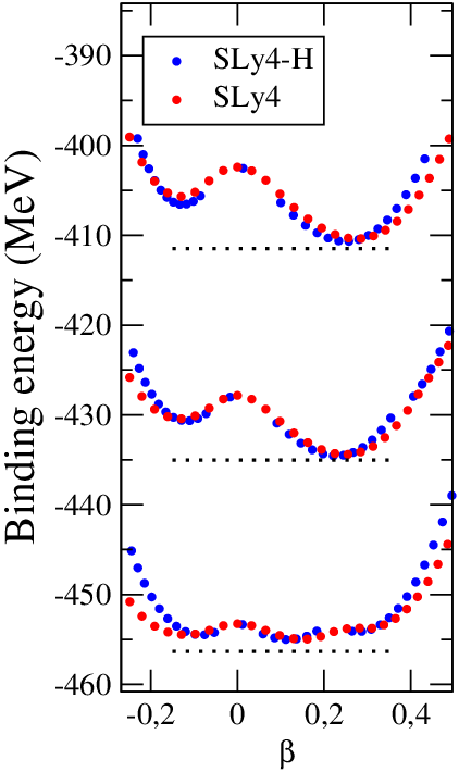
The strength of the quadrupole interaction is determined by fitting the cost of deforming. Thus we fix the quadrupole-quadrupole strength in the following manner: (i) for several values of the deformation parameter we compute the energy obtained with the functional within a Skyrme HF calculation with constraints on the quadrupole moment, (ii) is then fitted such that the HF energies obtained with the effective Hamiltonian (1), reproduces . As seen in Fig. 1 the cost of deforming can be reproduced in a reasonable way. The approximation of only having a single quadrupole term limits the range of deformations that can be described. Thus the agreement is expected to deteriorate for larger deformations where more complex shapes become important.
For the pairing part of the Hamiltonian (Eq. (4)) the interaction strength is determined applying the uniform model of (Nilsson and Ragnarsson 1995). This treatment of pairing is similar to the one in the Cranked-Nilsson-Strutinsky-Bogoliubov model (CNSB) (Carlsson et al. 2008b). First we assume the empirical estimate of the average gap, (Bohr et al. 1969a). The reduction factor of 0.7 comes from compensating for the effect of particle–number projection (Olofsson et al. 2007; Idini et al. 2015). Then, the strength is found by solving the uniform model (Nilsson and Ragnarsson 1995). For each nucleus we obtain different strengths by solving separately for protons and neutrons,
| (12) |
where the pairing window is set to MeV in the spherical basis. Here denotes the level density averaged in the energy window taken from the spherical HF solution. Note that the left hand side is modified to take into account the contribution of the exchange term in the pairing. The full treatment of the exchange term is needed to avoid the singularities when applying the projection operator and gives an extra contribution when breaking a pair (see appendix of (Carlsson et al. 2008b)).
In the way described in this section, all the coupling constants of the effective Hamiltonian becomes determined from the underlying reference functional. In this article we consistently apply the SLy4 parametrization of the Skyrme interaction (Chabanat et al. 1998) as a reference functional and denote the resulting Hamiltonian SLy4-H.
II.3 Collective coordinates
In the previous sections, we defined the effective Hamiltonian and its parameters. In the following, we define the many-body basis within which the Hamiltonian is solved. Our basis states consists of HFB vacua obtained with the effective Hamiltonian for several values of the deformation located on a grid. This grid is constructed by solving the HFB equations for the Hamiltonian in Eq. (1) with constraints on,
| (13) | ||||
| (14) |
with the expectation value of the operator respect to the deformed HFB states and . From this, one obtains the familiar , which defines the degree of quadrupole deformation, and , which defines the trixiality. We also use the cranking method with a constraint on,
| (15) |
In addition, we also include a variation of the pairing strengths and by scaling the pairing gaps . The many-body basis states are obtained as the lowest energy solutions to the HFB equations in a grid of , and values. The grids are generated by sampling a region of the plane. Each point of the plane can be associated with a certain value of . We have allowed a few different values of each of these variables and randomly assigned one of these values for each point. Only HFB states below a certain cut-off energy are kept and accepted as basis states.
This choice of generating coordinates attempts to account for the most important collective degrees of freedom namely: collective vibrations in the quadrupole degrees of freedom, rotations and pairing correlations. In order to improve the accuracy for a larger class of states in the spectrum one would need to enlarge the basis further by, for instance, including states built through quasiparticle (qp.) excitations. An equivalent way of introducing such non-collective particle-type excitations that is more in the spirit of the GCM is to act on the basis states with an excitation operator:
| (16) |
where is a normalization constant and is a two-quasiparticle creation operator:
| (17) |
The elements are chosen as
| (18) |
with , for to ensure symmetry. For each many-body state and for each matrix element, is randomly taken as . The value of is obtained from a parameter as,
| (19) |
The smallest value of the sum of the lowest qp. energies; for either protons or neutrons are used for both particle species in this relation.

The operator acts separately on neutron and proton parts of the states with the result that the lowest two-quasiparticle excitations are added to the states with weights determined by the parameter . Multi-quasiparticle excitations will also be added due to the structure of the series but with diminishing weights. The random sign ensures that even if the energy surface is over sampled the states will still have orthogonal components allowing for the extraction of more independent solutions. The quasiparticles are taken to have preserved parity and signature (=) quantum numbers. The quasiparticle pairs in Eq. (17) are restricted to belong to the group with positive parity and signature so that when acting on an HFB state, the generated excitations do not change the symmetry of the state. That is, the matrix elements can be characterized by the quantum numbers of the quasiparticle pairs and these are restricted to have positive signature and parity and to be of the same nucleon species. After acting on one of the basis states, the new state obtained contains a mixture of multi-quasiparticle excitations with random signs that reduces overcompleteness of the basis. In this way, this temperature inspired method introduces particle type excitations into the basis in order to complement the more collective excitations introduced through the generating coordinates.
An example is shown in Fig. 2. As seen from this figure the application of the excitation operator allows for a much larger number of eigenstates to be found and an improved convergence of the yrast band.
II.4 Efficient symmetry restoration
After generating the many-body basis, the following step consists in computing the matrix elements for the projected overlap and Hamilton operator.
By construction, the HFB vacua do not have either a good number of nucleons or angular momentum. As a consequence, it is necessary to introduce projection operators to restore symmetries and evaluate states with definite values for quantum numbers. The matrix elements read,
| (20) | ||||
| (21) |
| (22) |
where are projection operators for neutron, proton number, and angular momentum. are the rotations over the gauge and Euler angles, with the corresponding weights (see e.g. (Enami et al. 1999; Bally and Bender 2021)). From each HFB state one can often project out several many-body states with different projections. The final energies are invariant with respect to the orientation in the laboratory frame, so these matrix elements do not depend on the quantum number.
The computation of the matrix elements above is time consuming due to the projection operators, which involve angular integrations over angles in space and gauge space. As a consequence, it is essential to be able to perform accurate and systematic truncations in the computations of these matrix elements. Our truncation scheme is based on the Bloch Messiah decomposition, which allows to rewrite the Bogoliubov matrices and as , where and are both unitary matrices and defines the so-called canonical basis associated with the Bogoliubov vacuum (Ring and Schuck 1980). and can be chosen as diagonal and skew-symmetric, respectively. The matrix is written in terms of blocks of dimension with elements (, -) where is the occupation probability of the canonical basis state (the matrix elements of are such that ). Our truncation criteria is defined by first sorting the occupation numbers in descending order (see (Carlsson and Rotureau 2021)) and then truncating the canonical basis, that is we consider a smaller size where is such that
| (23) |
The occupation numbers differ for each state so each state is thus truncated differently and stored in the smaller representation before calculation of the matrix elements. The truncated states thus define our new basis states where long tails and numerical noise have been removed. Using these truncated states, the overlaps of rotated Bogoliubov states are computed and all the calculations are reduced to the minimal occupied subspace using the Bloch Messiah transformation (see (Carlsson and Rotureau 2021; Ring and Schuck 1980; Yao et al. 2009) and Appendix A).
An unpaired HFB vacua will have a dimension corresponding to the number of particles and exact zeros outside of this space. Paired vacua will have varying dimension depending on the pairing distribution. It is thus essential to be able to calculate overlaps of states having very different sizes. While the applied overlap formula allows the calculations of overlaps when states have ’s exactly equal to zero it also allows to reduce the dimension by keeping only non-zero ’s thus keeping only the essential information and therefore greatly reducing the computational time (Carlsson and Rotureau 2021).
II.5 Odd numbers of nucleons
The computation for nuclei with an odd number of nucleons proceeds similarly to the even-even case. In this paper, we consider the case of even-odd nuclei. Having generated the set of HFB vacua as described in the previous section, the odd-state basis is generated as a set of one quasiparticle creation operators acting on the HFB states, namely:
| (24) |
The corresponding Bogoliubov matrices and are easily obtained by replacing the column in and by the corresponding column in , Ring and Schuck 1980. Obviously, as in the case of even nuclei, the ability to truncate in a systematic manner is also critical for an efficient computation in the odd case. In this context, the computation of the overlap for odd system is performed using the truncated formula in Carlsson and Rotureau 2021. The application of the Bloch Messiah decomposition allows to rewrite the odd vacua as a product of three matrices
| (25) | |||||
| (26) |
where and are unitary matrices and,
| (27) |
The structure of and is almost identical to the even-even case except for the “odd” particle, which is unpaired. This unpaired particle is, by convention, placed in the first position in both matrices. The truncations of matrices can then proceed similarly as in the even case. That is, the truncation is dictated by the values of the paired particles. After decomposing the matrices in this form the calculation of projected Hamiltonian matrix elements proceeds similarly as in the even case (see appendix A).
II.6 Hill-Wheeler equation
The spectra are obtained by solving the Hill-Wheeler (HW) equation (Ring and Schuck 1980). The state solutions of the HW equations are, by construction, eigenstates of the parity and angular momentum operators and .
In matrix form the Hill-Wheeler equation reads,
| (28) |
with from Eq. (22), from Eq. (20) and where and are the resulting eigenvector and eigenvalue solutions. This equation can be solved separately for each total angular momentum giving energies and corresponding eigenstates as expansions in terms of the projected HFB states:
| (29) |
In this equation, are the HFB-basis states and the operators are projection operators for proton number, neutron number and angular momentum. The coefficients are found from the Hill-Wheeler equation in the basis of projected HFB-states and scaled such that becomes normalized.
II.7 Transitions and Quadrupole Moments
Because angular momentum projection is performed, the model gives eigenstates in the laboratory system as output. This makes it natural and straightforward to calculate observables avoiding the process of extracting them from the internal system; which inevitably contains approximations.
Furthermore, since the model allows for calculations in large model spaces there is no need for effective charges.
II.7.1 Reduced transition probability
Because of the interaction between the charged nucleus and the electromagnetic field, it is possible to have transitions between eigenstates of the nuclear Hamiltonian by emitting (or absorbing) a photon. Those transitions can be classified into electromagnetic multipoles. For a given multipole of order the emitted (absorbed) photon will carry a total angular momentum of .
The transition rate (the life time is given by ) from an initial to a final nuclear eigenstate for an electrical multipole is given by (Ring and Schuck 1980), in SI-units
| (30) |
where is the energy of the emitted photon. This expression is derived from "Fermi’s golden rule" up to first order in perturbation theory.
Due to the fact that quadrupole deformations are the dominant shape degrees of freedom for atomic nuclei, the quadrupole mode is the most prominent one for the radiation. Hence, here we will consider -transitions.
A nuclear eigenstate has definite values for the total angular momentum and its projection . Often one do not want to distinguish between different -values; neither for final nor initial states. Therefore one averages over initial (assuming an equal distribution of initial -values) and sum over final (the final -value is not important). This type of rate is therefore given by (for )
| (31) | ||||
where the reduced transition probability has been defined. The -values do not contain the large gamma-ray energy dependence of the transition rate. Therefore, calculations of the reduced transition probability are more easily compared to experiment than the transition rate.
II.7.2 Projection and GCM
In the model presented in this paper, projections onto good particle number and angular momentum are performed. In this approach, the :th state for given and can be written as in Eq. (29).
With those states, the matrix element for the reduced transition probability becomes,
| (32) | ||||
Where it has been used that conserves particle number. In reference Enami et al. 1999 it is stated that,
| (33) |
where the :s are Clebsch-Gordan coefficients with notation such that the two angular momenta in the subscript couple to the angular momenta in the superscript. Hence, in total we get
| (34) | ||||
In the expression for the -value, Eq. (31), the summations over and only involves the first Clebsch-Gordan coefficient in the above matrix element. Using orthogonally relations for the Clebsch-Gordan coefficients, the sum reduces to
| (35) |
The final expression for the reduced transition probability is then
| (36) | ||||
In the cases where measurements exists, we also compare the spectroscopic quadrupole moment, defined as:
| (37) |
This is defined in the laboratory frame and becomes identically zero for .
III Results
To test the developed model, calculations have been performed for five nuclei: Four even-even nuclei, the three chromium isotopes 48,50,52Cr, 24Mg and the even-odd 49Cr. The formalism of extracting the -transitions and the quadrupole moment has been implemented only for even-even nuclei. The results are compared both with experiment and with other theoretical calculations.
The chromium isotopes have been chosen in order to test the model when going from the deformed 48Cr to the more spherical 52Cr.
The experimental values for energies and transitions are taken from (Exp 2021) if not otherwise stated. Experimental values for the spectroscopic quadrupole moments are rare but the few found are from (Stone 2016). Some of the transition rates have not been explicitly given in ref. (Exp 2021), but are instead extracted from gamma energies and lifetimes according to Eq. (31). In the case where the state decays in several channels, the lifetime for channel , , can be calculated from the gamma intensity, , with the expression
| (38) |
where the sum goes over all channels.
III.1 Generation of collective subspace for the different nuclei
The points in the grid are defined by starting at spherical shape. For each new point the angle is increased with the golden angle . The radial distance is increased with the square root of the number of points. This generates a rather homogeneously sampled circular area in the plane. With cranking included, the surface will have mirror symmetry in the axis. An example for 48Cr with is shown in

Fig. 3. As seen from this figure 48Cr has a prolate minimum centered around with . As is increased this minimum will move towards where the rotation eventually becomes non-collective since the shape is then rotationally symmetric around the cranking axis (-axis).
For the pairing we use a grid in two variables and . These grids are constrained to four values: . These values specify scaling of the pairing values. A value of would imply generating the surface with only the self consistent pairing. While a value of 1.4 implies generating basis states with a stronger interaction that gives 1.4 times larger pairing gaps.
For the cranking frequency we choose a grid of three different values and the values needed for each state to obtain those values are estimated as (Nilsson and Ragnarsson 1995). The moment of inertia is estimated as in (Bengtsson and Åberg 1986), where for simplicity we used MeV for all points. For each point in the plane values of and are randomly drawn from the allowed sets in order to create states that sample the relevant many-body space. For the even-even nuclei we have used basis states with signature and for the odd 49Cr we compare the use of both .
In the numerical calculation of the excitation operator (Eq. (16)) we have used ( see Eq. (19)). This implies that for the particle species that is easiest to excite the lowest two-quasiparticle excitation within the considered symmetry group is added to the state with a weight of 0.45.
For all even-even chromium isotopes, the same calculation parameters have been used (values for 49Cr and 24Mg are given below). That is, 12 major shells in the harmonic oscillator basis generated by an updated version of the code hosphe Carlsson et al. 2010. The -plane has been sampled with 300 states within and . Since we are interested in the low-energy part of the spectra it is sufficient to consider basis states up to a given cutoff. Therefore only states within 12 MeV from the state with the lowest calculated energy has been kept, which is sufficient to cover the energy range of the experimental yrast states. This resulted in basis sizes of 198, 217 and 206 for the 48Cr ,50Cr and 52Cr isotopes, respectively. For the numerical computation of the projections, 10 points have been used in the number projections for both types of nucleons and (9, 18, 36) points in the angles for the angular momentum projection. These number of points for the angular momentum projection are obtained after applying symmetries to reduce the integration interval and corresponds to (36, 36, 36) points in the full space, see e.g. (Enami et al. 1999; Bally and Bender 2021).
The -values are calculated for every transition that differ with 2 or 0 units of spin. However, with few exceptions discussed, only transitions over 10 W.u are plotted in the spectra.
III.2 48Cr
The spectra for Cr24, both the calculated and the experimental values, together with the strongest transitions, are shown in Fig. 4. The calculation shows the characteristic of a rotor, , for the yrast band up to spin where the first backbending happens.

The general behavior of a deformed and rotating nucleus approaching a terminating states has been discussed in reference (Afanasjev et al. 1999). For a low angular momentum the rotation is of a collective nature with the rotation axis perpendicular to the symmetry axis of the nucleus. With increasing angular momentum the valence nucleons tend to align their spins with the rotation axis. This continues until all valence nucleons are fully aligned with the rotation axis. Then no further angular momentum can be built and one has reached the terminating state. In that state the rotation axis is parallel with the symmetry axis and therefore the rotation is of a single particle nature.
In 48Cr, the termination is expected to happen at . This can be understood from the fact that 48Cr has four protons and four neutrons in the subshell. Aligning all valence nucleons within this subshell results in spin .
The evolution of the internal structure of 48Cr with angular momentum up to its terminating state has been investigated in reference (Juodagalvis et al. 2000) within the cranked Nilsson-Strutinsky (CNS) model. The conclusion in that paper is that the intrinsic deformation goes from axially symmetric prolate over triaxial shapes to end up in a slightly oblate shape when the terminating state is reached.
Comparisons of transitions and quadrupole moments between results from our model and results obtained from CNS is shown in Fig. 5. Also three shell model (SM) calculations for three different interactions in the full -space are included (Poves 1999; Robinson et al. 2014; Hasegawa et al. 2000).

The results from our Hamiltonian, denoted SLy4-H, are in agreement with the previous CNS and SM calculations. Both the - and the -curves resembles the ones for a rigid rotor up spin . For higher angular momentum, the -values are approaching zero; showing that the states are indeed of a single particle nature rather than a mixed collective one. There is also a good agreement for the prediction of the properties of the spectroscopic quadrupole moment (37). All the models predict a quite drastic change in the shape associated with the backbend at and that the nucleus becomes close to spherical at the terminating state.
In a nucleus, as for 48Cr, it is expected that neutron-proton pairing should play an important role. This is because both the protons and the neutrons occupy the same valence space. Thus, they have maximal spatial overlap, cf. reference (Goodman 1999) for a discussion of neutron-proton pairing, the different types from the different isospin channels and their possible effects. Even though our model does not include neutron-proton pairing, it is interesting to compare the backbending from the calculations with experiment.

It can be seen in Fig. 6 that the backbending in SLy4-H occurs at the same spin and have the same magnitude as in experiment. However, the gamma energies are consistently lower for all angular momenta (except at the backbending). This is in line with references (Poves 1999; Robinson et al. 2005). In both those papers they separate out the neutron-proton pairing in the isospin channel from the rest of the pairing to see its effect. They both find that, without this pairing, the spectra becomes suppressed. This would imply a shift to the left for the backbending curve in Fig. 6 with around 0.2 - 0.5 MeV.
III.3 49Cr
We now focus on the even-odd Cr25 isotope. Shell model calculations in the shell have shown a good reproduction of the g.s. band and its rotational patterns at low spin can be described by the Particle-Rotor model as a band based on the [312]5/2- Nilsson orbital (Martinez-Pinedo et al. 1997).
Figure 7 shows the computed energies of states in the g.s. band of 49Cr in several bases. The results in panel a) of Fig. 7 are obtained, without cranking, in a basis of 116 states whereas for the results in panel b) and c), the cranking is included and the number of basis states is 114 and 156, respectively. Without cranking, the states in the odd basis with opposite signature are related by time-reversal and consequently the computed energies are identical whether the basis states have a signature or . This is not the case anymore when the cranking is included and we show in the panels b) and c) of Fig. 7 results for both signatures. All parameters are the same as for 48Cr and for each calculation, the basis is formed by blocking the qp. (see Eq. (24)) with the lowest energy 11 1 Due to the application of the excitation operator (16) on the HFB vacua, the qp.’s are no longer eigenstates for a finite value of . Nevertheless, the qp. with the lowest energy computed before the application of the operator (16), is selected to construct the odd state basis. This is justified by the fact that for low value, the ordering of the average qp. energy is not dramatically affected..
A general property is that states with are best described within a basis with signature and states with are best described within a basis with (Bohr et al. 1969b). However, from Fig. 7 one notices that the difference in the energies computed with the different signatures diminishes when the basis increases. It is then more natural to consider as the most precise energy for a state of angular momentum , the lowest energy among the two energies computed in the largest basis with and . As one can see in Fig. 7, the difference in the g.s. energy obtained with and is keV for the basis made of 114 states (panel b) and decrease to less than 150 keV in the larger basis (panel c). It is also worth noting that the difference between the lowest computed g.s. energies with cranking (panels b and c) and the g.s. energy without cranking (panel a) is keV.
Taking the lowest state in the bigger basis we obtain a binding energy MeV ( that is the energy of the g.s. in panel c) of Fig. 7 in the basis with ), which is slightly lower than the experimental binding energy MeV. In order to gain some insights into the amount of correlations included beyond the mean-field, it is instructive to compare with the lowest mean-field energy among the basis states. For each odd state , we can assign a mean-field energy , with the HFB-energy of the even-even vacuum and the energy of the qp. . In that particular case, the lowest mean-field energy among the basis states is MeV, which implies that the beyond mean-field effects included in the theory, lower the energy by MeV.
We show in Fig. 8, a comparison between the computed excitation energies and the experimental data. As one can see, the data are well reproduced by the calculation. In particular, our calculations reproduce the occurrence of a backbending for spin . The g.s. rotational band splits into two branches corresponding to sequences of states . As one can see in Fig. 8 at low spin, the two branches are close to each other and start to diverge for larger .

III.4 50Cr
The spectrum for Cr26 is given in Fig. 9. We calculated up to spin , which is expected to be the terminating spin of the ground state configuration.

The calculations reproduce the two lowest states that are very close in energy and that are also seen in experiment. In fact, the calculations suggest that the ground state band, which starts from the first -state, continues up to via the state. The yrast states for , and seem to originate from a different band. This is further confirmed from the spectroscopic quadrupole moments in Fig. 10. At they change sign, indicating a change in the internal structure.
Experiments also show a stronger -transition from the state than from the state. Unfortunately, there are no data of transition strengths for higher spin states above the yrast band.
For the purpose of this paper, CNS calculations for 50Cr have been performed. The results from those calculations can be used to interpret the internal structure of the states. It was found that the state indeed gets its angular momentum from collective rotation; in the same way as the lower part of the yrast band does. Whereas the state is predicted to be prolate with the symmetry axis parallel to the rotational axis. This implies that the rotation is built up by single particles spins.
Furthermore, the CNS calculations predict two more bands with positive parity. One band is located around 2.2 MeV above the yrast band and is built upon a excitation of the neutrons. This band is in fact divided into two nearly degenerated bands with opposite signature. Another excited band is found around 3.7 MeV above the yrast band and is built upon a neutron excitation.
As seen in Fig. 9, our model produce the same band structure as the CNS calculations. Hence, for this nucleus, the two methods are consistent with each other.
In experiments no excited bands with positive parity and even spins have yet been identified.
In Fig. 10 our results for the transitions and spectroscopic quadrupole moments are compared with experiment and shell model calculations for three different interactions (Martínez-Pinedo et al. 1996; Robinson et al. 2005; Hasegawa et al. 2000).

It is interesting to note the discrepancy between experiment and all of the shown theoretical calculations for the -value. Also, the experimental value is not what one would expect from a rotational model. In fact, the transitions for 48Cr also do not follow a rotor description for low angular momenta. But for that nucleus it is the value that is high. So, for both 48Cr and 50Cr the ratio is less than 1. This in contrast of the rotational model where the ratio is 1.43; which is in more agreement with the calculations. This discrepancy has been pointed out before (Hertz-Kintish et al. 2014). In reference (Wang 2020) it is suggested the that unusual ratio can be understood in a collective picture with the inclusion of appropriate three-body forces. This is shown explicitly for 170Os in the interacting boson model.
III.5 52Cr
In Cr28 the eight valence neutrons fill up the orbit and therefore the nucleus is expected to be less deformed and close to a spherical shape. And, indeed, both experiment and our calculations show a spectra in which the yrast band is more similar to a linear vibrational one than to a quadratic rotational one, see Fig. 11.

The calculated energies for the yrast band fits well with experiment up to the expected termination at . In contrast, the model does not agree with experiment for the yrast states with larger angular momenta; too high energies are obtained. However, the angular momenta, which are assigned to those states from experiment, are considered uncertain. Our calculations support the possibility that these states have a different angular momenta than the ones they have been attributed.
In experiment, two rotational bands with positive parity and even spins have been identified. The ground state band up to spin and a second band built from the -state which goes up to spin . And as seen from the transitions in Fig. 11, our model indeed predicts a rotational band just above the yrast band. The calculated second band starts at the -state and passes over the - and -states. For the calculated transitions between the bands are strong. This indicates a similar internal structure of the two bands for low angular momenta.
Those two bands, the shell closure yrast band and the excited rotational band, have been investigated by Caurier et al. (Caurier et al. 2004). They found that the yrast band indeed is composed mainly by the closed shell configuration. In contrast, the excited rotational band is built upon the -state with an internal structure dominated by two neutrons above the orbital. In addition, they calculate and values for the excited band which are compared in Fig. 12 with our results. Also, in Fig. 12, the results for the yrast band is compared with a SM-calculation (Hasegawa et al. 2002). While there is a good overall agreement between theory and experiment our calculations predict the bands slightly closer in energy and more mixed than in experiment for .

III.6 24Mg
The main reason to test the model on the nucleus Mg12 is to compare the results with the ones presented in references (Bender and Heenen 2008) and (Rodríguez and Egido 2010). In those references they use a similar procedure as the one given in this paper. That is, a mean field basis of HFB-states with different constraints on the -deformations, projections onto good quantum numbers and mixing using the GCM.
The main difference is that those works use the same interaction throughout the whole calculation; SLy4 in (Bender and Heenen 2008) and Gogny D1S in (Rodríguez and Egido 2010). Since those forces are density dependent it is not well defined how to perform the mixing of states. Therefore, the density is replaced with the transition density to overcome this problem. It has been pointed out that this procedure can lead to poles in the energy for some deformations (Bender et al. 2009). This issue is absent in our model since we postulate a Hamiltonian which can be used in a straightforward way in the mixing. Our results, together with experiment, are shown in Fig. 13 and in Fig. 14 values and quadrupole moments are compared both with experiments and the previous calculations.
The parameters of the calculation for 24Mg are the same as for the chromium isotopes except for the following: 10 major shells in the harmonic oscillator single-particle basis, 300 states to sample the -plane within and . Keeping states below 25 MeV in excitation energy resulted in 133 basis states. The number of points for the projections are 10 for the particle numbers of both types of nucleons and (6, 12, 24) for the angels of the angular momentum (corresponding to (24, 24, 24) points in the full space). The cut-off value for the displayed transitions is 7 W.u.

For the spectra, the Gogny force succeeds to reproduce experimental values in an excellent way, at least up to . To the advantage of our model is that it reproduces the yrast state below the rotational band; which is seen in experiment. This state is not reported in (Rodríguez and Egido 2010).
The state has also been reproduced in SM-calculations and in the CNS-method; both presented in reference (Sheline et al. 1988). In that paper, using the CNS method, it is found that this state is maximally aligned with its symmetry axis parallel to the axis of rotation. Hence, it is predicted to be a non-collective state. Indeed, this is expected to happen at which is the maximal spin that can be produced for the four valence particles confined to the orbits of character. In contrast, the state, which belongs to the ground state band, is of a collective nature with the axis of rotation perpendicular to the symmetry axis. This ground state band continues until it terminates at (Sheline et al. 1988). Note the similarity with 50Cr where the aligned state is yrast for , while the ground band terminates for .

Also for the transitions the results from (Bender and Heenen 2008) and (Rodríguez and Egido 2010) fits well with experiment. Again at least up to . But the trend that the -values increase with higher spin seems questionable. It is not what one would expect; neither from experiment nor from experience for rotational bands approaching a terminating state. Our model agree more with shell model calculations and have the expected decrease with spin.
IV Conclusions
The method introduced works surprisingly well for the description of both spectra and transitions. Both transitions and delicate structure information such as backbending are correctly reproduced for all nuclei considered. Defining a Hamilton operator allows the many-body calculations to be carried out in a straightforward manner, without any need for additional assumptions to treat the density-dependent parts of the functional. In this work, the postulated separable Hamiltonian is constrained to reproduce the energy surface of a reference EDF. Correctly describing the detailed landscapes of energy minima and corresponding shapes is one of the basic components needed in order to reproduce the experimental spectra. We have chosen the effective Hamiltonian as simple as possible, while still capable of producing realistic results. The simplicity of the interaction, together with the reduction to the smallest space using the Bloch–Messiah method, allows for advanced many-body calculations. We have incorporated both collective and single-particle type excitations using around 200 HFB vacua in the basis. The number of points needed in the angular momentum projection increases rapidly when considering higher angular momentum states (Johnson and O’Mara 2017) and in this work the calculations have been carried out to spin 16 while maintaining the refined many-body mixing of the states. This allowed to cover the spin range up to the terminating states seen in these nuclei. Thus, to obtain in the complete space a fully symmetry restored description of the gradual transition from collective rotation to the non-collective terminating states based on the GCM.
The present results give encouraging prospects for the future. Any nuclear interaction can be expressed in terms of sums of separable terms, through e.g. a singular value decomposition or more refined physically motivated expansions Tichai et al. 2019; Nesterenko et al. 2002. Thus, the simple expansion explored here can be fully developed into a converging expansion. The question in this respect is the applicability and efficiency of the method. The present study demonstrates the numerical efficiency of the approach. The effective Hamilton operator employed here may still be extended with more terms while keeping the calculations feasible. The first such terms to consider could be an improved pairing part, hexadecapole terms in the particle-hole part, and a refined treatment of Coulomb.
Acknowledgments
B.G.C. and J.L. thank the Knut and Alice Wallenberg Foundation (KAW 2015.0021) for financial support. J.R thank the Crafoord foundation for support. A.I. was supported by Swedish Research Council 2020-03721. We also acknowledge the Lunarc computing facility.
References
- Skyrme (1958) T. Skyrme, Nuclear Physics 9, 615 (1958), ISSN 0029-5582, URL https://www.sciencedirect.com/science/article/pii/0029558258903456.
- Carlsson et al. (2008a) B. G. Carlsson, J. Dobaczewski, and M. Kortelainen, Phys. Rev. C 78, 044326 (2008a), URL https://link.aps.org/doi/10.1103/PhysRevC.78.044326.
- Raimondi et al. (2011) F. Raimondi, B. G. Carlsson, and J. Dobaczewski, Phys. Rev. C 83, 054311 (2011), URL https://link.aps.org/doi/10.1103/PhysRevC.83.054311.
- Ryssens and Bender (2021) W. Ryssens and M. Bender, Phys. Rev. C 104, 044308 (2021), URL https://link.aps.org/doi/10.1103/PhysRevC.104.044308.
- Bender et al. (2003) M. Bender, P.-H. Heenen, and P.-G. Reinhard, Rev. Mod. Phys. 75, 121 (2003), URL https://link.aps.org/doi/10.1103/RevModPhys.75.121.
- Scamps et al. (2021) G. Scamps, S. Goriely, E. Olsen, M. Bender, and W. Ryssens, Eur. Phys. J. A 57, 333 (2021), URL https://doi.org/10.1140/epja/s10050-021-00642-1.
- Veselý et al. (2012) P. Veselý, J. Toivanen, B. G. Carlsson, J. Dobaczewski, N. Michel, and A. Pastore, Phys. Rev. C 86, 024303 (2012), URL https://link.aps.org/doi/10.1103/PhysRevC.86.024303.
- Carlsson et al. (2012) B. G. Carlsson, J. Toivanen, and A. Pastore, Phys. Rev. C 86, 014307 (2012), URL https://link.aps.org/doi/10.1103/PhysRevC.86.014307.
- Carlsson and Ragnarsson (2006) B. G. Carlsson and I. Ragnarsson, Phys. Rev. C 74, 044310 (2006), URL https://link.aps.org/doi/10.1103/PhysRevC.74.044310.
- Delaroche et al. (2010) J. P. Delaroche, M. Girod, J. Libert, H. Goutte, S. Hilaire, S. Péru, N. Pillet, and G. F. Bertsch, Phys. Rev. C 81, 014303 (2010), URL https://link.aps.org/doi/10.1103/PhysRevC.81.014303.
- Nomura et al. (2020) K. Nomura, R. Rodríguez-Guzmán, and L. M. Robledo, Phys. Rev. C 101, 014306 (2020), URL https://link.aps.org/doi/10.1103/PhysRevC.101.014306.
- Alhassid et al. (2006) Y. Alhassid, G. F. Bertsch, L. Fang, and B. Sabbey, Phys. Rev. C 74, 034301 (2006), URL https://link.aps.org/doi/10.1103/PhysRevC.74.034301.
- Carlsson et al. (2013) B. G. Carlsson, J. Toivanen, and U. von Barth, Phys. Rev. C 87, 054303 (2013), URL https://link.aps.org/doi/10.1103/PhysRevC.87.054303.
- Dönau (1998) F. Dönau, Phys. Rev. C 58, 872 (1998), URL https://link.aps.org/doi/10.1103/PhysRevC.58.872.
- Bender et al. (2009) M. Bender, T. Duguet, and D. Lacroix, Phys. Rev. C 79, 044319 (2009), URL https://link.aps.org/doi/10.1103/PhysRevC.79.044319.
- Carlsson and Rotureau (2021) B. G. Carlsson and J. Rotureau, Phys. Rev. Lett. 126, 172501 (2021), URL https://link.aps.org/doi/10.1103/PhysRevLett.126.172501.
- Såmark-Roth et al. (2021) A. Såmark-Roth, D. M. Cox, D. Rudolph, L. G. Sarmiento, B. G. Carlsson, J. L. Egido, P. Golubev, J. Heery, A. Yakushev, S. Åberg, et al., Phys. Rev. Lett. 126, 032503 (2021), URL https://link.aps.org/doi/10.1103/PhysRevLett.126.032503.
- Kumar and Sørensen (1970) K. Kumar and B. Sørensen, Nuclear Physics A 146, 1 (1970), ISSN 0375-9474, URL https://www.sciencedirect.com/science/article/pii/0375947470910821.
- Nilsson and Ragnarsson (1995) S. Nilsson and I. Ragnarsson, Shapes and Shells in Nuclear Structure (Cambridge University Press, Cambridge, 1995).
- Idini et al. (2012) A. Idini, F. Barranco, and E. Vigezzi, Phys. Rev. C 85, 014331 (2012), URL https://link.aps.org/doi/10.1103/PhysRevC.85.014331.
- Potel et al. (2017) G. Potel, A. Idini, F. Barranco, E. Vigezzi, and R. A. Broglia, Phys. Rev. C 96, 034606 (2017), URL https://link.aps.org/doi/10.1103/PhysRevC.96.034606.
- Aguilar and Broglia (2021) G. P. Aguilar and R. A. Broglia, The Nuclear Cooper Pair: Structure and Reactions (Cambridge University Press, 2021).
- Tsunoda et al. (2020) N. Tsunoda, T. Otsuka, K. Takayanagi, N. Shimizu, T. Suzuki, Y. Utsuno, S. Yoshida, and H. Ueno, Nature 587, 66 (2020).
- Dudek et al. (1982) J. Dudek, Z. Szymański, T. Werner, A. Faessler, and C. Lima, Phys. Rev. C 26, 1712 (1982), URL https://link.aps.org/doi/10.1103/PhysRevC.26.1712.
- Perez et al. (2017) R. N. Perez, N. Schunck, R.-D. Lasseri, C. Zhang, and J. Sarich, Computer Physics Communications 220, 363 (2017), ISSN 0010-4655, URL https://www.sciencedirect.com/science/article/pii/S0010465517302047.
- Carlsson et al. (2008b) B. G. Carlsson, I. Ragnarsson, R. Bengtsson, E. O. Lieder, R. M. Lieder, and A. A. Pasternak, Phys. Rev. C 78, 034316 (2008b), URL https://link.aps.org/doi/10.1103/PhysRevC.78.034316.
- Bohr et al. (1969a) A. Bohr, B. Mottelson, W. B. (Firm), Ray, and C. C. S. Collection, Nuclear Structure: Volume I (single-particle motion), Nuclear Structure (Basic Books, 1969a), ISBN 9810239793.
- Olofsson et al. (2007) H. Olofsson, R. Bengtsson, and P. Möller, Nuclear Physics A 784, 104 (2007), ISSN 0375-9474, URL https://www.sciencedirect.com/science/article/pii/S0375947406009043.
- Idini et al. (2015) A. Idini, G. Potel, F. Barranco, E. Vigezzi, and R. A. Broglia, Phys. Rev. C 92, 031304 (2015), URL https://link.aps.org/doi/10.1103/PhysRevC.92.031304.
- Chabanat et al. (1998) E. Chabanat, P. Bonche, P. Haensel, J. Meyer, and R. Schaeffer, Nuclear Physics A 635, 231 (1998), ISSN 0375-9474, URL https://www.sciencedirect.com/science/article/pii/S0375947498001808.
- Exp (2021) Evaluated nuclear structure data file (2021), URL http://www.nndc.bnl.gov.
- Enami et al. (1999) K. Enami, K. Tanabe, and N. Yoshinaga, Phys. Rev. C 59, 135 (1999), URL https://link.aps.org/doi/10.1103/PhysRevC.59.135.
- Bally and Bender (2021) B. Bally and M. Bender, Phys. Rev. C 103, 024315 (2021), URL https://link.aps.org/doi/10.1103/PhysRevC.103.024315.
- Ring and Schuck (1980) P. Ring and P. Schuck, The nuclear many-body problem (Springer-Verlag, New York, 1980).
- Yao et al. (2009) J. M. Yao, J. Meng, P. Ring, and D. P. Arteaga, Phys. Rev. C 79, 044312 (2009), URL https://link.aps.org/doi/10.1103/PhysRevC.79.044312.
- Stone (2016) N. J. Stone, Atomic Data and Nuclear Data Tables 111 (2016), ISSN 0092-640X, URL https://www.osti.gov/biblio/22917909.
- Bengtsson and Åberg (1986) R. Bengtsson and S. Åberg, Physics Letters B 172, 277 (1986), ISSN 0370-2693, URL https://www.sciencedirect.com/science/article/pii/0370269386902510.
- Carlsson et al. (2010) B. Carlsson, J. Dobaczewski, J. Toivanen, and P. Vesely, Computer Physics Communications 181, 1641 (2010).
- Afanasjev et al. (1999) A. Afanasjev, D. Fossan, G. Lane, and I. Ragnarsson, Physics Reports 322, 1 (1999), ISSN 0370-1573, URL https://www.sciencedirect.com/science/article/pii/S0370157399000356.
- Juodagalvis et al. (2000) A. Juodagalvis, I. Ragnarsson, and S. Åberg, Physics Letters B 477, 66 (2000), ISSN 0370-2693, URL http://dx.doi.org/10.1016/S0370-2693(00)00214-8.
- Poves (1999) A. Poves, Journal of Physics G: Nuclear and Particle Physics 25, 589 (1999), URL https://doi.org/10.1088/0954-3899/25/4/004.
- Robinson et al. (2014) S. J. Q. Robinson, T. Hoang, L. Zamick, A. Escuderos, and Y. Y. Sharon, Phys. Rev. C 89, 014316 (2014), URL https://link.aps.org/doi/10.1103/PhysRevC.89.014316.
- Hasegawa et al. (2000) M. Hasegawa, K. Kaneko, and S. Tazaki, Nuclear Physics A 674, 411 (2000), ISSN 0375-9474, URL https://www.sciencedirect.com/science/article/pii/S0375947400001718.
- Goodman (1999) A. L. Goodman, Phys. Rev. C 60, 014311 (1999), URL https://link.aps.org/doi/10.1103/PhysRevC.60.014311.
- Robinson et al. (2005) S. J. Q. Robinson, A. Escuderos, and L. Zamick, Phys. Rev. C 72, 034314 (2005), URL https://link.aps.org/doi/10.1103/PhysRevC.72.034314.
- Martinez-Pinedo et al. (1997) G. Martinez-Pinedo, A. P. Zuker, A. Poves, and C. E, Physical Review, C 55 (1997), URL https://www.osti.gov/biblio/435262.
- Bohr et al. (1969b) A. Bohr, B. Mottelson, W. B. (Firm), Ray, and C. C. S. Collection, Nuclear Structure: Volume Ii (nuclear Deformations), Nuclear Structure (Basic Books, 1969b), ISBN 9780805310160.
- Martínez-Pinedo et al. (1996) G. Martínez-Pinedo, A. Poves, L. M. Robledo, E. Caurier, F. Nowacki, J. Retamosa, and A. Zuker, Phys. Rev. C 54, R2150 (1996), URL https://link.aps.org/doi/10.1103/PhysRevC.54.R2150.
- Hertz-Kintish et al. (2014) D. Hertz-Kintish, L. Zamick, and S. J. Q. Robinson, Phys. Rev. C 90, 034307 (2014), URL https://link.aps.org/doi/10.1103/PhysRevC.90.034307.
- Wang (2020) T. Wang, EPL (Europhysics Letters) 129, 52001 (2020), URL https://doi.org/10.1209/0295-5075/129/52001.
- Caurier et al. (2004) E. Caurier, F. Nowacki, and A. Poves, Nuclear Physics A 742, 14 (2004), ISSN 0375-9474, URL http://dx.doi.org/10.1016/j.nuclphysa.2004.06.032.
- Hasegawa et al. (2002) M. Hasegawa, K. Kaneko, and S. Tazaki, Progress of Theoretical Physics 107, 731 (2002), ISSN 0033-068X, eprint https://academic.oup.com/ptp/article-pdf/107/4/731/5342884/107-4-731.pdf, URL https://doi.org/10.1143/PTP.107.731.
- Bender and Heenen (2008) M. Bender and P.-H. Heenen, Phys. Rev. C 78, 024309 (2008), URL https://link.aps.org/doi/10.1103/PhysRevC.78.024309.
- Rodríguez and Egido (2010) T. R. Rodríguez and J. L. Egido, Phys. Rev. C 81, 064323 (2010), URL https://link.aps.org/doi/10.1103/PhysRevC.81.064323.
- Fifield et al. (1978) L. Fifield, M. Hurst, T. Symons, F. Watt, C. Zimmerman, and K. Allen, Nuclear Physics A 309, 77 (1978), ISSN 0375-9474, URL https://www.sciencedirect.com/science/article/pii/0375947478905365.
- Sheline et al. (1988) R. K. Sheline, I. Ragnarsson, S. Aberg, and A. Watts, Journal of Physics G: Nuclear Physics 14, 1201 (1988), URL https://doi.org/10.1088/0305-4616/14/9/008.
- Johnson and O’Mara (2017) C. W. Johnson and K. D. O’Mara, Phys. Rev. C 96, 064304 (2017), URL https://link.aps.org/doi/10.1103/PhysRevC.96.064304.
- Tichai et al. (2019) A. Tichai, R. Schutski, G. E. Scuseria, and T. Duguet, Phys. Rev. C 99, 034320 (2019), URL https://link.aps.org/doi/10.1103/PhysRevC.99.034320.
- Nesterenko et al. (2002) V. O. Nesterenko, J. Kvasil, and P.-G. Reinhard, Phys. Rev. C 66, 044307 (2002), URL https://link.aps.org/doi/10.1103/PhysRevC.66.044307.
- Bonche et al. (1990) P. Bonche, J. Dobaczewski, H. Flocard, P.-H. Heenen, and J. Meyer, Nuclear Physics A 510, 466 (1990), ISSN 0375-9474, URL https://www.sciencedirect.com/science/article/pii/037594749090062Q.
Appendix A Computation of Matrix elements
The Hamiltonian matrix elements in Eq. (22) can be expressed (Ring and Schuck 1980),
| (39) |
The contribution of the two-body interaction in Eq. (1) to the particle-hole fields becomes
| (40) |
and the contribution to the particle-particle fields becomes:
| (41) |
In order to speed up the calculations it is important to reduce the dimensions to the minimal occupied subspace (Yao et al. 2009; Bonche et al. 1990). We choose a block size which is the maximum value of and (see Eq. (23)) to denote the size of the upper left block in the equations below. The BM transformation is used to transform the matrices of the vacua. As an example for the vacua we obtain and with
The transitional densities and (Ring and Schuck 1980) can then be transformed and expressed:
with
| (48) | ||||
| (49) | ||||
| (50) | ||||
| (51) | ||||
| (52) |
where
| (53) |
and
| (54) |
For the blocks of the transformed interaction we introduce the notation:
| (55) | ||||
| (56) | ||||
| (57) | ||||
| (58) | ||||
| (59) | ||||
| (60) |
If we furthermore decompose the all matrices into proton and neutron parts and use to label the proton or neutron blocks we obtain the full expression for the matrix elements in the optimal space and with proton and neutron parts explicitly written out as:
Where in addition we have used the symmetries of our interaction:
In the code, this expression is further optimized by moving as many operations as possible outside the loops of gauge and Euler angles. The effect of symmetry restoration does not change the canonical occupation numbers but only leads to a matrix multiplication acting on the matrix.