Complex Langevin approach to interacting Bose gases
Abstract
Quantitative numerical analyses of interacting dilute Bose-Einstein condensates are most often based on semiclassical approximations. Since the complex-valued field-theoretic action of the Bose gas does not offer itself to the direct application of standard Monte Carlo techniques, simulations beyond their scope by now almost exclusively rely on quantum-mechanical techniques. Here we explore an alternative approach based on a Langevin-type sampling in an extended state space, known as complex Langevin (CL) algorithm. While the use of the CL technique has a long-standing history in high-energy physics, in particular in the simulation of QCD at finite baryon density, applications to ultracold atoms are still in their infancy. Here we examine the applicability of the CL approach for a one- and two-component, three-dimensional non-relativistic Bose gas in thermal equilibrium, below and above the Bose-Einstein phase transition. By comparison with analytic descriptions at the Gaussian level, including Bogoliubov and Hartree-Fock theory, we find that the method allows computing reliably and efficiently observables in the regime of experimentally accessible parameters. Close to the transition, quantum corrections lead to a shift of the critical temperature which we reproduce within the numerical range known in the literature. With this work, we aim to provide a first test of CL as a potential out-of-the-box tool for the simulation of experimentally realistic situations, including trapping geometries and multicomponent/-species models.
I Introduction
Interacting Bose-Einstein condensates are at the center of contemporary experimental as well as theoretical studies. Though much of the interest nowadays focuses on non-equilibrium properties, many open questions still remain for Bose gases in equilibrium. A tremendously successful description of the weakly interacting Bose gas is provided by Bogoliubov theory Pitaevskii and Stringari 2016. However, there are many situations of interest where Bogoliubov theory is not very straightforward or even unfeasible to apply. These include Bose gases in trapping potentials Giorgini et al. 1996, in lower dimensions Hutchinson and Blakie 2006, with spin interactions Stamper-Kurn and Ueda 2013 and at phase transitions, to name only a few.
For such scenarios it would be convenient to have a method at hand to simulate the Bose gas from first principles. Unfortunately, the field theoretic path integral describing the Bose gas in equilibrium may not be simulated by straightforward Monte Carlo methods because the action is complex in general, an obstacle known as sign problem and plaguing numerical computations in a wide range of physical scenarios Henelius and Sandvik 2000; Lombardo 2007; Alford and Kryjevski 2010; Aarts 2009.
One possibility to circumvent this problem is to avoid the field theoretic (coherent state) path integral description of the non-relativistic Bose gas altogether. This approach is pursued by the path integral Monte Carlo (PIMC) technique Pilati et al. 2006; Spada et al. 2022, which treats the problem of interacting bosons in a quantum-mechanical rather that a field-theoretic framework. This method provides exact simulations also for strongly interacting bosons, while its computational cost increases polynomially with the number of particles to be captured.
Other methods stick to the field-theoretic formulation, where there is no limitation on particle number, but employ a semi-classical approximation. These include the truncated Wigner Sinatra et al. 2002; Blakie et al. 2008 as well as the projected Gross-Pitaevskii equation (PGPE) algorithm Davis et al. 2001; Davis et al. 2002.
On the other hand, there are numerical methods available that promise to directly tackle the sign problem in the evaluation of path integrals. These include, inter alia, the diagrammatic Monte Carlo method Boninsegni et al. 2006; Van Houcke et al. 2010, the density of states algorithm Fodor et al. 2007; Gattringer and Langfeld 2016, the dual variables approach Endres 2007; Gattringer and Langfeld 2016 and the fixed node Monte Carlo method van Bemmel et al. 1994; Foulkes et al. 2001; Rothstein et al. 2019. Two particularly promising, completely general and model-independent approaches are the Lefschetz thimbles Cristoforetti et al. 2012; Pawlowski et al. 2021 as well as the complex Langevin (CL) algorithm Parisi 1983; Klauder and Petersen 1985; Seiler, Erhard 2018. Both involve the artificial complexification of real fields, thereby doubling the number of degrees of freedom of the original problem, somewhat similar in spirit to the positive P-representation approach Gilchrist et al. 1997; Deuar and Drummond 2006a; Deuar and Drummond 2006b.
In this work we will focus on the complex Langevin algorithm. The method has a long-standing history in the simulation of lattice QCD at finite chemical potential Aarts and Stamatescu 2008; Sexty 2014; Kogut and Sinclair 2019; Ito et al. 2020. More recently, it has also found applications in condensed matter physics, mainly in the simulation of non-relativistic fermions Loheac and Drut 2017; Rammelmüller et al. 2018. In contrast, works applying CL in the context of bosonic ultracold atoms are scarce, with the notable exception of Hayata and Yamamoto 2015; Attanasio and Drut 2020.
By performing a systematic study of the three-dimensional interacting Bose gas we here want to demonstrate that CL can also be a useful tool for simulations of ultracold bosonic atoms, in particular because it provides a possibility to perform exact simulations within the field-theoretic description of interacting bosons. This paves the way for evaluating observables in equilibrium Bose-Einstein condensates of arbitrary particle number from first principles, without the need of employing any approximation scheme.
II The complex Langevin method
The path integral
| (1) |
for a theory described by the action for the variable or field , generalizes the partition sum in statistical mechanics and thus offers itself for the numerical evaluation of observables according to
| (2) |
In contrast to classical statistical mechanics, where the measure involves a positive-definite probability distribution, the action in the quantum path integrals (1) and (2) is in general, however, not real-valued. This renders a straightforward Monte Carlo evaluation of the expectation value (2) unfeasible, an obstacle known as the sign problem. Many, by order of magnitude large, but positive and negative contributions can contribute to the sum, both in the real and imaginary parts, to give an eventually comparatively small result. Evaluating this sum generically is exponentially hard Berger et al. 2021.
A particular approach developed for tackling this difficulty is the complex Langevin (CL) method Berger et al. 2021. It exploits the well-known equivalence between path integrals and the stochastic Langevin equation as well as the fact that the latter can be formulated also for complex actions. The Langevin approach is well established in statistical mechanics, corresponding to the case of a real-valued action describing, in the simplest case, the dynamics of a real-valued field . Expectation values of the form (2) can be computed by evolving the field along a fictitious time according to the stochastic Langevin equation
| (3) |
with being a Wiener noise averaging to and subject to the Markovian covariance , and by taking the average of along the direction of . Eq. (3) can be discretized as
| (4) |
with the being Gaussian random variables with zero mean and standard deviation and being the discretization of the Langevin time.
The CL method extends this scheme for the case of a complex action . Observing that Eq. (3) leads into the complex plane even for the case of a real-valued field , one complexifies each field component, , which are evolved according to twice as many Langevin equations as before,
| (5) | ||||
| (6) |
with the noise being subject to
| (7) | ||||
Hence, the CL equations involve, in general, a stochastic force in both the real and imaginary directions. The two noise contributions must fulfill the condition in order ensure that the path integral involves a single integration “direction” as in a line integral Kades et al. 2022. It has been shown, however, that it is numerically most convenient to set and Aarts et al. 2010.
While it is a straightforward exercise to demonstrate the equivalence of the Langevin approach to the original path integral for real actions, its validity in the case of complex actions cannot be established rigorously. It is known to fail in certain cases, either because of the occurrence of runaway trajectories in the complex plane or because the process converges to an unphysical result Aarts et al. 2010; Hayata et al. 2016; Nishimura and Shimasaki 2015, which both represent characteristic consequences of the sign problem. Several methods have been developed to at least ameliorate the problem of runaways Aarts and James 2010; Seiler et al. 2013; Attanasio and Jäger 2019; Alvestad et al. 2021. Furthermore, there is substantial numerical evidence that the method can indeed give reliable results in a broad range of physical settings Berger et al. 2021. While the sign problem eventually traces back to the unevadable complexity of Hilbert space, there have been several attempts to settle the issue by defining criteria for the correctness of the method Gausterer and Lee 1993; Aarts et al. 2010; Nagata et al. 2016; Salcedo 2016; Scherzer et al. 2019; Scherzer et al. 2020.
In this paper we rather adopt a hands-on approach and test the complex Langevin approach at the exemplary system of a dilute Bose gas in three dimensions above and below the condensation phase transition. Since the upper critical dimension of the dilute Bose gas is , the three-dimensional system is expected to be well-described by mean-field theory close to the phase transition, and thus also further away from it. Hence we evaluate momentum distributions and dispersion relations at different chemical potentials and compare them to analytical predictions from quantum field theory at the mean-field level, using the Bogoliubov and Hartree-Fock approximations below and above the transition, respectively. We moreover explore the more intricate properties near the phase transition and reproduce the shift of the critical temperature within the limits reported in the literature.
In this way we can demonstrate that the CL method represents a promising and easy-to-implement technique for computing many-body observables for interacting bosonic quantum gases in thermal equilibrium. The method can be straightforwardly extended to trapped configurations, multiple components and more intricate interaction terms, and in principle also lower dimensions where quantum correlations are expected to play a stronger role and are expected to provide a more stringent test bed of the method.
Since CL is not the only method in the context of ultracold bosonic atoms that employs Langevin-type field equations, some remarks about other stochastic approaches to Bose-Einstein condensates are in order. These mainly include methods based on the positive-P representation, which were already mentioned above, as well as the stochastic Gross-Pitaevskii equation (SGPE) Stoof and Bijlsma 2001; Gardiner et al. 2002; Gardiner and Davis 2003; Cockburn and Proukakis 2009; Gautam et al. 2014. What distinguishes CL from both of them is that it attempts to directly compute the Feynman path integral. The stochastic dynamics thus takes place in a fictitious, unphysical time, during which the Langevin process explores the space of field configurations, i.e., samples from the possible values of the quantum field at each point in space and physical time (the physical time can be either imaginary as in thermal equilibrium or real as in non-equilibrium). In contrast, both the positive-P method and the SGPE are formulated in the physical time of the system, and the stochastic dynamics can be regarded as an actual physical evolution. A further distinctive feature of CL which it shares with the positive-P method but not with the SGPE approach is that it attempts to transform the computationally hard problem of sampling from a non-positive-definite distribution (as it arises generally when one wants to perform full quantum simulations) to sampling from a positive-definite distribution in a phase space with twice as many degrees of freedom. Thus, for a complex Bose field , both CL and the positive-P method require to evolve four real fields instead of two. In contrast, the SGPE does not feature any artificial extension of the number of degrees of freedom. The stochastic term here arises from the coupling of the condensate to the cloud of thermally excited particles. By virtue of including this interaction with the thermal background, the SGPE goes beyond a pure mean-field description, but it does not attempt to solve the full quantum problem from first principles and can rather be classified as a semi-classical method Gardiner and Davis 2003. In this regard it differs from CL and the positive-P approach, which both in principle provide exact simulations of the full quantum problem but are not applicable in all situations of interest due to the intrinsic and inevitable complexity of quantum physics.
III Complex-Langevin simulations of a thermal dilute Bose gas
III.1 The dilute -component Bose gas
We study a non-relativistic -component Bose gas with U symmetric interactions in thermal equilibrium at inverse temperature and chemical potential 11 1 Throughout the paper we use natural units where . The action, expressed in terms of the complex Bose fields , , defined on the -dimensional Euclidean manifold of imaginary time and position , reads
| (8) |
with Hamiltonian density
| (9) |
where summation over the field components, , is implied, and is the mass of the particles. For a dilute atomic gas in dimensions, the dimensionful coupling is commonly defined in terms of the -wave scattering length , while the relevant measure for the coupling strength is the dimensionless gas parameter
| (10) |
Being defined in terms of the average density of particles , it relates to the mean interparticle spacing and evaluates, in typical experimental settings, to a number on the order of . Hence, the model is weakly interacting and expected to be well described by low-order perturbative approximations, at least substantially below and above the condensation phase transition.
III.2 Observables
We are eventually interested in computing correlation functions of operators as
| (11) |
Since the action (8) is, in general, not purely real-valued due to the ”Berry phase” term , a straightforward Monte Carlo evaluation of the path integral (III.2) is unfeasible, which thus forms an exemplary problem we plan to tackle using the complex Langevin approach.
In the following, we will focus on uniform dilute Bose gases in cubic spatial volumes subject to periodic boundary conditions, such that we can evaluate observables most conveniently in momentum space. The main object we consider is the occupation number of the mode with wave number ,
| (12) |
where summation over is implied. Exploiting the homogeneity in direction, we average the -local expectation value over imaginary time in order to gain a higher statistical accuracy.
Close to the transition and in the condensate phase, is expected to be much larger than one, , for all modes in the semi-classical regime of momenta below the temperature scale , where also classical statistical methods such as the truncated Wigner approximation Sinatra et al. 2002; Polkovnikov 2010, or the PGPE algorithm Davis et al. 2001 are applicable. At larger momenta, however, where occupancies are small, , the quasi-classical approximation is expected to fail, and one needs either genuine quantum statistical methods or single-particle techniques as the path-integral Monte Carlo (PIMC) algorithm Pilati et al. 2006. The PIMC approach is formulated in a quantum-mechanical rather than a quantum field-theoretic framework and thus is limited to comparatively small total particle numbers. We will demonstrate that the CL method is applicable in both the strongly and the weakly occupied regimes.
For the single-component system, , we additionally extract the dispersion by evaluating
| (13) |
The dispersion will give a first measure of the energy of elementary excitations of the system. Also here, exploiting the homogeneity in direction, we average over in order to gain a higher statistical accuracy.
III.3 Implementation of the CL simulations
All our simulations of a one- () and a two-component () Bose gas were performed on an space-time lattice, with varying discretization along the imaginary-time direction, ranging between and . Details on the discretization of the action (8) and the derivation and form of the corresponding Langevin equations are provided in Appendix A. For simplicity, we fix the temporal units by choosing in terms of the inverse of the lattice spacing . The temperature and thus are then given in units of , fixing, for a given also the imaginary-time lattice length in units of . The Langevin time step is set to .
In each run, we prepared the system in some initial state, as described in the subsequent sections. For example, above the transition, we chose the vacuum state, setting at each point on the spatial and temporal lattice. We then propagated the discretized Langevin equations, details of which are provided in App. A. After a certain equilibration time that varies with the physical scenario, we can compute averages of the observables along the field trajectories.
The computational cost of a single Langevin time step scales as the total space-time lattice size. In addition to this, also the Langevin evolution time required to reach a fixed statistical precision scales as , such that the total computational cost scales as . The latter can be inferred from the fact that the action, discretized in direction, is of the form
| (14) |
where is the imaginary-time step size and the discretized Hamiltonian, cf. App. A for details. Increasing for fixed implies a correspondingly smaller drift term and thus a slower exploration of the space of field configurations, such that a longer Langevin evolution time is required for obtaining the same statistical accuracy.
In order to speed up the simulation, we parallelized the computation of the Langevin drift and the propagation of the field according to the Langevin equations on GPUs, in a way such that every GPU thread updates a single lattice point. Working on NVIDIA V100 cards, it takes about hours of wall time to evolve a one-component lattice for time steps and to extract the momentum spectrum after each time step. While for most scenarios we evolved for steps, we increased this number to steps for the simulations close to the transition in order to gain a higher statistical accuracy needed for the precise determination of the transition point.
Statistical errors are generally estimated from the variance of several independent runs. For further details on the numerical extraction of observables, see App. B.1.
III.4 Ideal gas – dependence on time discretization
Before we move on to evaluating the observables defined above for an interacting dilute Bose gas at and away from the condensation transition, we perform, as a first benchmark of our approach, CL simulations of an ideal Bose gas. We use this, in particular, to discuss the errors induced by the discretization of imaginary time, corresponding to a truncation of the Fourier representations beyond a highest Matsubara frequency.
For the ideal gas, the coupling vanishes, , and we tune the chemical potential to , above the phase transition, where the condensate fraction vanishes. We choose the temperature to be , which, together with corresponds to a total density and thus a critical temperature and a thermal de Broglie wave length of .
We simulate for a Langevin time of , and begin the averaging after an equilibration time . Additionally, we average over 10 independent runs. In each run, we prepare the system in the vacuum state, setting at each point on the lattice.

The resulting, angular averaged momentum distribution for is shown in Fig. 1. At large, the results for the distribution agree excellently with the analytic expression,
| (15) |
with free single-particle dispersion
| (16) |
over the whole range of momenta, while a weak deviation is seen at the smallest occupancies in the Boltzmann tail. We amplify this discrepancy by showing, in the inset, the relative deviation on the same logarithmic momentum scale.
As we recall from App. B.3, the occupation number of the ideal gas, on a discrete imaginary-time lattice, can be written as
| (17) |
We show the relative deviation as a dotted line in the inset of Fig. 1, which agrees on average with the deviation between the CL data and the exact result. This, in particular, demonstrates that the systematic increase of the relative numerical error in the low-occupancy region at large momenta can be attributed to the truncation of the Matsubara series.
In order to further corroborate this observation, we have performed runs with a different number of lattice points along the imaginary-time direction. The respective deviations and for , , are compared with each other in Fig. 2. As one can see, the deviation of the CL data from the exact Bose-Einstein distributions decreases with increasing , as predicted by the analytical finite- results shown as dashed lines.

The dispersion of the ideal Bose gas, , obtained as an angular average over (13), is shown for in Fig. 3. The continuum dispersion is given by the basic free-gas kinetic energy, shifted by the chemical potential,
| (18) |
while the finite-size dispersions result, as described in App. B.3, as
| (19) |

The deviation between the CL and continuum analytic results is visibly larger, but can be attributed, as for the momentum spectrum , to the finite lattice resolution in imaginary-time direction and thus to the corresponding truncation of the sum over the Matsubara frequencies. This is again corroborated by a comparison of the deviation for different , as shown in Fig. 4.

III.5 Interacting gas above the BEC phase transition
Having performed first benchmark computations for an ideal Bose gas, we now turn to a weakly interacting, i.e., dilute gas and use the complex Langevin approach to calculate momentum spectra and dispersions for chemical potentials and temperatures away from and near the condensation phase transition. We start with considering the case above the transition, where we can compare our numerical results to analytic predictions on the basis of the Hartree-Fock (HF) Gaussian approximation. Subsequently, we benchmark our CL results to Bogoliubov theory below the transition, for both one- and two-component systems. Finally, we will explore the vicinity of the phase transition, where we can obtain a benchmark beyond mean-field theory, by computing the relative shift of the critical temperature due to interactions, a quantity that is sensitive to non-Gaussian fluctuations.

Above the critical point, we use the CL approach to compute the observables for the same choice of temperature and chemical potential, but with a non-vanishing, positive coupling constant , quantifying the repulsive contact interactions between the bosons. Our simulations return, for the chosen parameters, a density of , where we have extracted as described in App. B. The corresponding diluteness parameter , Eq. (10), is found to be , which is within the range typically reached in cold-gas experiments. Note, that, with the basic implementation of the method as described here, in the grand-canonical ensemble formulation, we can freely choose temperature and chemical potential, while the mean energy and density are obtained from the numerical data. This procedure can be straightforwardly extended to systematically determine the Lagrange parameters from given mean thermodynamic quantities.
Fig. 5 shows the momentum spectrum of the dilute gas in analogy to the ideal-gas spectrum depicted in Fig. 1, on a lattice, with . The main panels demonstrates good agreement with results obtained within the Hartree-Fock (HF) approximation Dalfovo et al. 1999, as described in the following.
Expanding the Hamiltonian (9) in leading order of a mean-field approximation corresponds to replacing the quartic term by
| (20) |
Above the transition, we can neglect the in general complex anomalous densities such that the resulting Hamiltonian describes, again, a non-interacting Bose gas, albeit with a shifted chemical potential
| (21) |
The mean particle density , which equals the momentum integral over the Bose-Einstein distribution, hence must be determined self-consistently, that is, by solving the equation
| (22) |
To determine and from this , we numerically solve Eq. (22), evaluating the polylogarithm directly. We obtain which can be compared to the density obtained from our CL simulations as indicated above. The density corresponds to , which gives the ideal-gas Bose-Einstein distribution shown as the dashed line in Fig. 5, which significantly deviates from the dash-dotted distribution for .
The inset of Fig. 5 shows the relative deviation from the expected Hartree-Fock result and compares it to the deviation of the finite- from the version of the HF spectrum, on a temporal lattice of points. This demonstrates good agreement over the whole range of momenta.
III.6 Bose gas in the condensed phase
Before we move on to studying the region close to the BE phase transition, we repeat the previous analysis away from criticality, in the condensed phase. In a condensate, the pattern of possible collective excitations fundamentally changes due to spontaneous symmetry breaking. While the Hugenholtz-Pines (or Goldstone) theorem implies the elementary excitations to be gapless in the zero-energy limit, the interactions suppress density vs. phase fluctuations, such that long-range phase coherence prevails which renders the long-wave-length excitations sound like. In the case of more than one internal component of the U symmetric model (9), however, additional Goldstone excitations are possible, which correspond to relative density variations between the components. These excitations are not subject to the suppression by interactions, which depend on the total density only, and are therefore similar to the motion of non-interacting bosons. To explore our algorithm for this case, too, we consider, in the following, systems with both and .
III.6.1 One-component system
We start again with the single-component system, , for which we now choose a temperature , chemical potential , and coupling constant . This results in a total density of , corresponding to a diluteness . As before, we work on a lattice, with different choices of the imaginary-time size .
It turned out, though, that initializing the field as for the Langevin evolution, as we did for all runs above the phase transition, the Langevin process is not able to build up a condensate, i.e., a highly over-occupied mode even at temperatures far below the transition, at least not within the limited simulation time available. This could be expected for large systems as the relative size of the phase space covered by the condensate mode is inversely proportional to the system size.
When starting instead from a spatially uniform, non-vanishing field configuration given by the semi-classical mean-field value , the CL process leads to only a slight modification, which consists in a thermal depletion of the condensate mode and the buildup of the corresponding distribution of momentum excitations shown in Fig. 6.

From Bogoliubov mean-field theory one expects the momentum distribution of the single-component gas to be Pitaevskii and Stringari 2016
| (23) |
where
| (24) |
in which denotes the condensate density
| (25) |
with spatial volume . The Bogoliubov dispersion of the elementary excitations is given in terms of the free dispersion , Eq. (18), by
| (26) |
Note that the quasiparticle dispersion is sound like, , at momenta below the healing-length scale .
The second contribution to (23), , gives rise to the quantum depletion, i.e., it accounts for all particles that are not in the condensate mode due to the interactions even at . The first term, which is proportional to the thermal occupancy of the quasiparticles, approximated as being non-interacting, accounts for the fraction of particles, which are non-condensed due to thermal excitations.
In Fig. 6, we show the spectrum (23) as a black dashed line, which hardly deviates from our numerical data, as reflected by the relative deviation depicted in the inset. The grey dotted and dashed lines indicate the contributions to the analytic spectrum (23), which account for the thermal and quantum depletion of the condensate, respectively.
We estimate the deviation caused by a finite by replacing the thermal distribution of non-interacting quasiparticles in Eq. (23) by the finite- expression, as we did this for the ideal gas,
| (27) |
As can be inferred from the inset of Fig. 6, this captures the residual deviation between the CL and Bogoliubov distributions up to momenta above which the quantum depletion becomes more relevant than the thermal one.

In Fig. 7 we compare the deviations of the distributions obtained with CL and the Bogoliubov distribution with the respective deviations of the finite- estimate from the full Bogoliubov distribution, for three different . This demonstrates that the Matsubara series truncation also affects the region of high momenta where dominates the spectrum.


Also the Bogoliubov dispersion, which we show in Fig. 8, is well reproduced by the CL simulations.
Finally, it is important to note that the CL method is not only able to describe the part of the momentum spectrum which is dominated by thermal excitations but also to reproduce the occupation numbers at high momenta where the spectrum is dominated by the quantum contribution. In order to further corroborate this observation, we also performed a simulation for a much smaller temperature, , i.e., we increased to . For such low temperatures, the spectrum is almost entirely dominated by the quantum depletion. Still, the spectrum is accurately reproduced by CL, see Fig. 9. This gives hope that CL is a suitable tool for performing exact simulations also in the quantum regime.
III.6.2 Two-component system
We have repeated the above simulations for the case of a two-component system, with U symmetric Hamiltonian (9). From Bogoliubov theory (see App. C for a summary for the general U case), one obtains, as mentioned initially, besides the gapless elementary excitations of the total density with dispersion (25), an additional free Goldstone mode with dispersion given by (18) for each of the remaining degrees of freedom. For the case of general , the total momentum distribution reads
| (28) |
where
| (29) |
We show the results of our CL simulations in Fig. 10 and compare them to the total Bogoliubov distribution (III.6.2), as well as to the quantum and thermal contributions from the Bogoliubov and free modes, respectively.

III.7 Interacting system at the transition
We finally would like to explore the CL approach to the dilute Bose gas close to the Bose-Einstein phase transition. We start by considering the occupation number spectrum to show a pure Rayleigh-Jeans power law in the IR as a signature of the phase transition, before we move on to determining the shift of the critical temperature due to interactions in the real Bose gas.
III.7.1 Rayleigh-Jeans scaling
At the transition, we expect the occupation number to show Rayleigh-Jeans scaling,
| (30) |
for small in the infinite-volume limit. In principle, this could provide a method for determining the transition point, which, in practice, however, is suited only for obtaining a rough estimate of where the phase transition occurs. On the one hand, statistical errors are in general large for the relevant small momentum modes; on the other hand, in finite-size systems, even at the transition, Rayleigh-Jeans scaling is not expected to be realized down to vanishing momenta.
As reported in the previous section, the formation of a condensate by the Langevin process can take unrealistically long computation times. Hence, for simulations below the transition, a condensate must be seeded by choosing a non-vanishing zero-mode population in the initial configuration for the Langevin process. However, since we do not know a priori at which chemical potential condensation occurs, it is most convenient to approach the critical point from the non-condensed phase. Nonetheless, the fact that the Langevin equilibration time strongly increases for a condensed state gives us a further (numerical) indication for determining the transition point.
We choose a temperature and a coupling , resulting in a density and thus a diluteness of . From HF theory, one obtains the transition to occur at , with the critical density in the free system. This amounts to for chosen temperature and coupling.
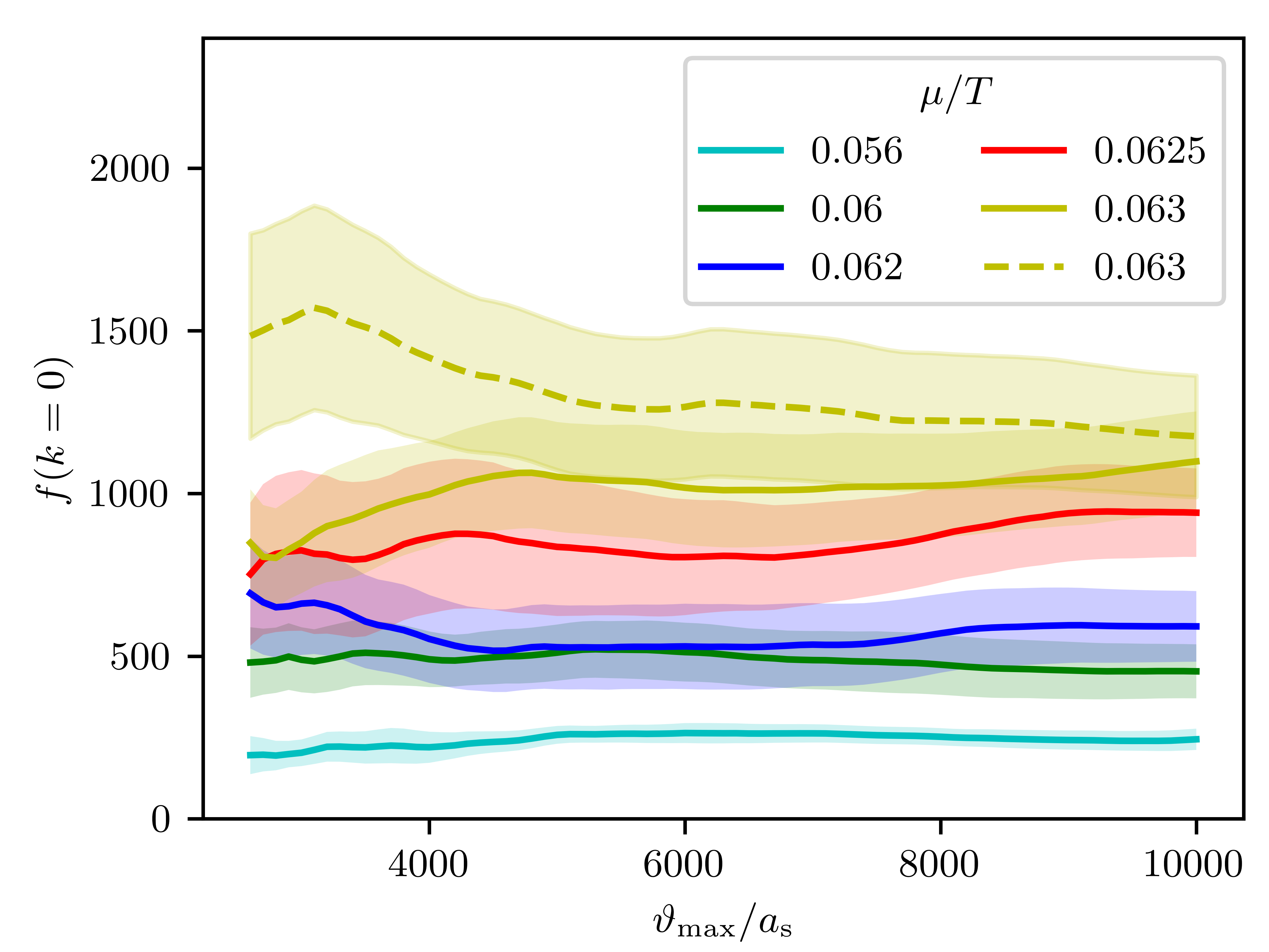
We perform simulations for five values of the chemical potential between and . The Langevin time evolution of the accumulated average of the zero-mode occupancy,
| (31) |
is shown in Fig. 11, as a function of the maximum Langevin time and for . While we observe a fast convergence in for and , i.e. still rather far away from the transition, the convergence of appears to be more and more slowed down for , , and , especially for the latter value of the chemical potential, giving a first hint that the system approaches the transition. In order to make sure that our results are reliable and not biased by insufficient simulation time, we performed additional runs with a non-zero seed of , corresponding to , for the case of the largest chemical potential, . The error bands indicate the variance over independent runs and thus illustrate the demand for statistics in the zero mode. The long-time zero-mode occupancy appears to converge for all chemical potentials and especially the two simulations with different seed for are consistent with each other within the error bands. All runs used in the remainder of this chapter have been performed without a seed in the zero-mode.

III.7.2 Shift of the critical temperature
Let us now turn to the determination of the shift of the transition temperature due to interactions. At leading order in the dimensionless interaction strength, set by the diluteness , Eq. (10), the shift scales as Baym et al. 1999, and to next-to-leading order in , it takes the form Arnold et al. 2001
| (32) |
where , , and are numerical constants, is the critical temperature of the ideal Bose gas in dimensions and the shift of its value in the presence of interactions.
While, in principle, a thorough determination of the transition point requires carefully extrapolating to the infinite-volume limit, for the case of a weakly interacting gas we can employ a somewhat simpler approach. Consider the condensate fraction in a free gas as a function of , for a fixed temperature , and system size , and thus fixed ratio of the system size and the thermal wave length . Varying the chemical potential allows tuning the total density as well as the zero-mode density , and the critical temperature , such that
| (33) | ||||
| (34) |
where is the fugacity. The total particle number as a function of in the continuum limit can be determined as the sum
| (35) |
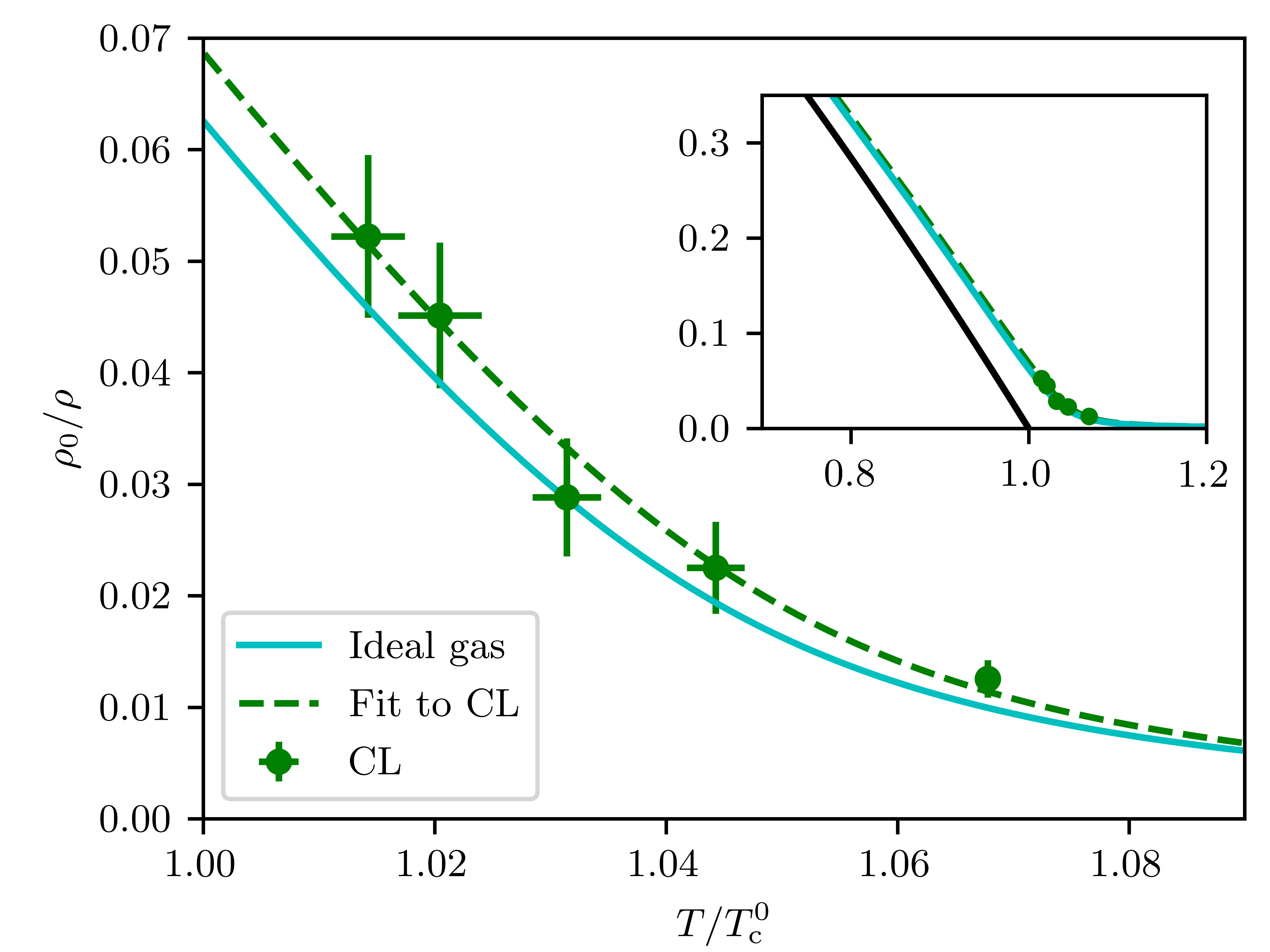
where the sums are performed over , with chosen large enough to ensure convergence. The resulting dependence of the ideal-gas condensate fraction on is shown in Fig. 13 as a solid cyan line. For comparison, the inset shows the same curve over a wider range near the critical temperature, together with the critical scaling (black solid line), which results in the thermodynamic limit .
For the weakly interacting Bose gas, we make use of the approximation, that the functional form of the condensate fraction as a function of in units of the critical temperature is the same as in the non-interacting case, albeit with a shifted critical temperature, i.e.
| (36) |
with and thus . Within errors, this is confirmed by our data. For each of the chemical potentials chosen in our CL simulations, we determine the total density from the sum over the occupation number spectrum over all points of the momentum-time lattice, which we correct by the difference between the continuum and lattice densities determined for the ideal gas at the same temperature and chemical potential, see App. B.4 for details. In this way, we determine condensate fractions and corresponding values of for the five different near-critical considered above, which we can compare, cf. Fig. 13, with the behaviour of the ideal gas in the continuum.
A least-squares fit of the ideal-gas curve to the simulation data (dashed green line) yields an interaction-induced shift of the critical temperature of
| (37) |
Possible finite-size corrections to this result are discussed in App. D. For the density at the diluteness becomes . As a consequence, neglecting the -corrections in (32), the constant in Eq. (32) takes the value
| (38) |
The determination of the constant has a long and controversial history Stoof 1992; Grüter et al. 1997; Holzmann et al. 1999; Reppy et al. 2000; Arnold and Tomášik 2000; Arnold and Moore 2001; Kastening 2004; Nho and Landau 2004, see Andersen 2004 for a review. Within the errors, our result (38) is in good agreement with the value (no error provided) from Holzmann et al. 1999, while it is larger than from the PIMC simulations of Grüter et al. 1997 and smaller than the average of more recent results which accumulate near , compare from Arnold and Moore 2001, from Kashurnikov et al. 2001 (Monte Carlo simulation of classical field theory), from Kastening 2004 (variational perturbation theory), and from Nho and Landau 2004 (PIMC simulation). Experiments with helium in Vycor glasses have found Reppy et al. 2000, while this has been disputed in Arnold and Tomášik 2000.
We also note that in Arnold et al. 2001 the constants and , which quantify the corrections to (32) of order were determined. The authors found , and , which for our diluteness yield an -correction to the shift and a total shift of , which is to be compared with (37). In order to distinguish numerically the leading-order and next-to-leading order contributions would require an analysis for a range of different densities or interaction strengths and thus dilutenesses, which is beyond the scope of the present work.
In summary, our analysis demonstrates that the CL method gives access to a beyond mean-field quantity (in the mean-field approximation, there is no shift of the transition temperature), consistent with previous results by order of magnitude.
IV Conclusion and Outlook
We have shown that it is possible to evaluate the coherent-state path integral of the interacting Bose gas from first principles by means of the complex Langevin (CL) method in experimentally relevant coupling regimes. We found that the spectra and dispersions obtained via the Hartree-Fock and Bogoliubov approximations are well reproduced above and below the transition, respectively. By determining the shift of the critical temperature due to interactions, we could show that the method is in principle capable of providing corrections beyond mean-field approximations. This opens a perspective on possibilities of using CL for ab initio simulations of interacting Bose gases in a wide range of experimental settings.
A remaining potential challenge is using the method in the regime of strong coupling strengths. Here we find CL to perform very well in the experimentally relevant regime of dilute gases, with diluteness parameter , without the need for additional improvements such as adaptive time step size or regulators. Notwithstanding this, choosing a diluteness of one order of magnitude higher (, corresponding to a by two orders higher particle density), we encounter runaways into the complex plane of field values, which are typical for the method in parameter regimes, in which the so-called sign problem prevails. While such highly dense Bose gases are experimentally difficult to realize, it remains an interesting task beyond the scope of our work to determine the limits up to which the CL method leads to meaningful results in an efficient manner.
For dilute systems, the method promises to be useful in many different contexts, e.g., trapped systems beyond the local density approximation Goldman et al. 1981, two-dimensional gases near the BKT transition Foster et al. 2010; Prokof’ev et al. 2001, or spinor gases beyond the U-symmetric case Stamper-Kurn and Ueda 2013, for exploring the phase diagram in comparison with mean-field predictions Kawaguchi et al. 2012; Kawaguchi and Ueda 2012, or the exploration of anomalous averages and their interplay with the gaplessness of the spectrum Yukalov and Kleinert 2006. In principle, one may consider CL also for simulating real-time path integrals and thus time evolving systems. This, however, poses a far more challenging sign problem, so far providing access to short-time evolution only Berges et al. 2007.
V Acknowledgments
The authors thank Felipe Attanasio, Marc Bauer, Iacopo Carusotto, Stefanie Czischek, Pjotr Deuar, Martin Gärttner, Christof Gattringer, Lukas Kades, Jan Pawlowski and Axel Pelster for discussions and collaboration on related topics. This work is supported by the Deutsche Forschungsgemeinschaft (DFG, German Research Foundation) under Germany’s Excellence Strategy EXC 2181/1- 390900948 (the Heidelberg STRUCTURES Excellence Cluster), under SFB 1225 ISOQUANT - 273811115, as well as grant GA677/10-1. The authors furthermore acknowledge support by the state of Baden-Württemberg through bwHPC and the German Research Foundation (DFG) through grant INST 35/1134-1 FUGG (MLS-WISO cluster) and grant no INST 40/575-1 FUGG (JUSTUS 2 cluster).
APPENDIX
Appendix A Discrete Langevin equations
In this appendix, we provide details of the discretization of the action (8) and the complex Langevin equations (5) derived from it.
We express the complex Bose fields in terms of its real and imaginary parts as
| (39) |
Discretizing these components on the lattice, , etc. for , the action (8) can be written as
| (40) |
where the index enumerates the imaginary time lattice sites with spacing , the three-dimensional index vector the spatial lattice sites, with discretization . is the Laplacian on the lattice, i.e.
| (41) |
with the unit vectors in three dimensions. Note that must be evaluated infinitesimally later than , i.e. at lattice point rather than at , as can be seen from the construction of the coherent-state path integral where in each time step is evaluated with respect to the coherent state on the left while acts to the right, on the state one step earlier. This is important even in the analytical treatment where it ensures the right convergence in the complex Matsubara plane Altland and Simons 2010.
The corresponding Langevin equations are obtained from (A) by taking derivatives with respect to and ,
| (42) |
and
| (43) |
where
| (44) |
Note that both and must now be taken to be complex variables, such that the complex Langevin method requires to evolve four real fields per component instead of two as in classical GPE simulations.
Appendix B Numerical extraction of the observables
B.1 Spectrum and dispersion on the lattice
The translation of the occupation number to the lattice gives , where, as for the action, must be evaluated at the temporal lattice point and at , following from the construction of the coherent state path integral, cf. App. A. When computing the dispersion, more care is in order. In the operator formalism, we can write it as
| (45) |
The discretization of on the temporal lattice is somewhat subtle. Since translates to , one is tempted to naively write . This, however, does not correspond to the operator finite-time differences
| (46) |
which contain an anti-time-ordered term, and thus cannot be simply translated to .
Hence, a better choice is to discretize the product of derivatives as
| (47) |
which contains time-ordered terms only and implies the discretization
| (48) |
of the dispersion, which we finally sum over , in which is it homogeneous, to gain statistics.
B.2 Momentum and integrals over momentum
On a lattice of size , the kinetic energy associated with the momentum mode with indices is not given by as in the continuum. The discretization (41) of the Laplacian rather implies the energy to be sine-spaced, i.e.
| (49) |
Accordingly, the modulus of the momentum associated with mode reads
| (50) |
In computing and we perform angular averages and accumulate the momenta into bins of width . For the lowest 8 bins, which contain only a single value of , we use this value as the -coordinate in plots of functions of momentum, while for all other bins we choose the center of the bin.
Integrals over momentum space such as necessary for determining the mean density are evaluated as sums as
| (51) |
where we choose again such that the sums run over , and where is the occupation number of mode , averaged over imaginary time, cf. (12), i.e., summed over , cf. App. B.3. The factor in Eq. (51) containing cosines is a Jacobian that takes into account the sine-spacing of the lattice momenta.


B.3 Truncated Matsubara expansion of particle spectrum and dispersion
For the purpose of numerical simulations, the imaginary time interval must be discretized. Here we want to discuss in more detail the errors induced by this discretization. Consider, e.g., the expectation value of the particle number operator in mode , for a single-component gas.
In the continuum, dropping any momentum indices, the expectation value can be written as
| (52) |
Evaluating this expression in the number-state basis gives the Bose-Einstein distribution,
| (53) |
Within the path integral formulation, the thermal expectation value of the number operator is represented by an imaginary-time path integral, the discretized Feynman representation of which reads
| (54) |
with the time-discretized action ()
| (55) |
where the index is identified with the index .
Expanding the fields on the finite time interval in terms of Matsubara modes,
| (56) |
with the Matsubara frequencies , , the path integral (54) becomes
| (57) |
with
| (58) |
Performing the Gaussian integrals yields
| (59) |
One shows in a similarly way that the dispersion , defined in Eq. (48), for finite becomes
| (60) |
In the continuum limit, , the series (B.3) converges to . On the lattice, however, the series needs to be truncated at some finite , such that an error occurs which depends on , but also on the value of . Fig. 14 shows the numerically computed truncation error for several combinations of and . In the right panel, one sees that the relative error for small is positive but turns negative at some point and quickly becomes rather large (while the absolute error still decreases). This illustrates the needs in temporal resolution for a precise evaluation of small occupation numbers as well as of the corresponding dispersions, the limits of which can be seen in Figs. 1–8. In fact, for large enough , the relative error on the particle number can even become , as can be seen from Fig. 15, which shows a version of Fig. 1 including the part of the spectrum up to .

B.4 Finite-resolution corrections near criticality
On the computational lattice, systematic deviations of observables from their continuum counterparts are caused by both the finite number of Matsubara modes and the finite spatial lattice resolution. Both mainly affect the UV properties of the system and therefore, in describing the critical behaviour near the phase transition, are expected to give a small correction only. Furthermore, for a weakly interacting gas above the transition, the spectrum is well approximated by an ideal-gas Bose-Einstein distribution with a shifted chemical potential, see Sect. III.5. It is thus reasonable to account for the described systematic errors in the following way: For a free gas at in a box of fixed size , we numerically determine the deviation between the density on the lattice and in the continuum (but for finite system size ). is then added to the density determined from numerical data for the interacting system. For the parameters as chosen in Sect. III.7, i.e. a lattice at , we obtain . This is a rather small correction, but it is significant in determining the constant .
Appendix C Bogoliubov theory of the U symmetric Bose gas
In this appendix, we provide, for conciseness, some details on the Bogoliubov mean-field description of an -component Bose gas described by the U symmetric Hamiltonian (9). For a complete discussion in the context of spinor Bose gases, see, e.g., Refs. Kawaguchi and Ueda 2012; Stamper-Kurn and Ueda 2013. In momentum space, the “Kamiltonian” entering the grand-canonical ensemble, reads
| (61) |
where enumerate the different field components, is the coupling and the volume. Making the Bogoliubov ansatz and expanding to quadratic order in the non-zero mode operator, this becomes
| (62) |
where is the condensate density, which is chosen equal in each component, such that the total condensate density is . In order to diagonalize in the component degree of freedom, we introduce
| (63) | ||||
| (64) |
where the vectors form an arbitrary orthonormal basis of the dimensional orthogonal complement of the -component vector . Thereby we obtain
| (65) |
The equivalence of (C) and (C) can be easily seen by plugging the transformation (63) and (64) into (C) and exploiting the fact that and the form an orthonormal set. In leading-order mean-field approximation the energy is minimized at the chemical potential . Upon inserting this, (C) becomes
| (66) |
which describes Bogoliubov modes and free Goldstone excitations . The total occupation number for can then be written as
| (67) |
with Bogoliubov and free dispersions
| (68) | ||||
| (69) |
Appendix D Possible finite-size effects in the extraction of
In our extraction of the transition temperature shift due to interaction effects we refrained from performing a systematic finite-size analysis. Numerical results by Kashurnikov et al. 2001 (who performed such a systematic analysis and defined the shift in the finite system in a manner similar to ours) suggest that for the system size that was employed here ( thermal wave lengths ), finite size corrections are already significantly smaller than our statistical error. Namely, they find the shift of the critical temperature to scale with system size as
| (70) |
with , , 22 2 Note that, in Ref. Kashurnikov et al. 2001, constants were chosen in the factors multiplying and .. For our parameters and system size, we obtain from this formula a deviation of between the finite- and the value for the shift, which is only half our statistical error (), which justifies our procedure.
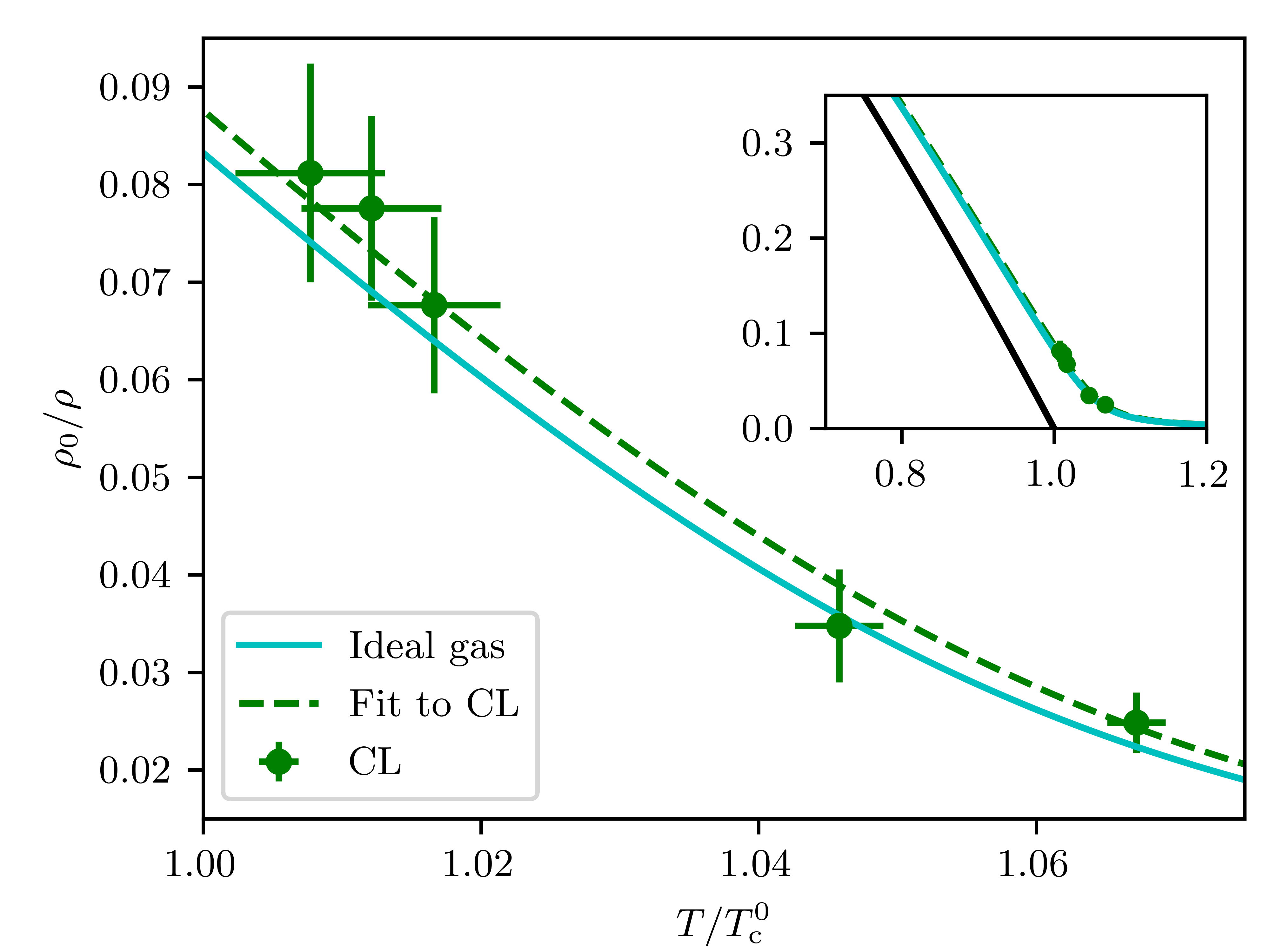
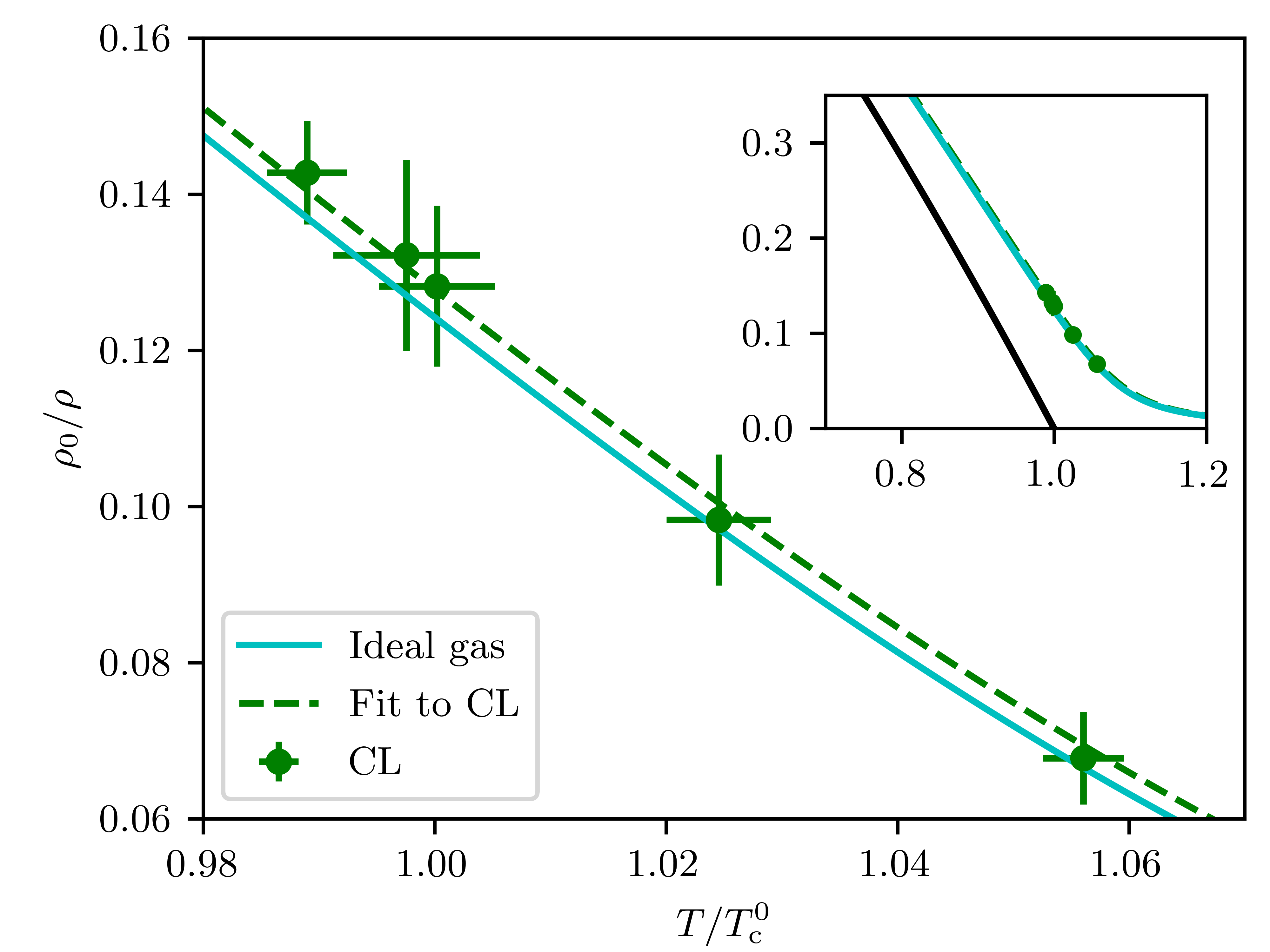
Our own simulations corroborate said weak dependence on . To demonstrate this, we perform the same analysis as in the main text but for the smaller and lattices, for the exact same chemical potentials. The result is shown in Fig. 16. Here we obtain for the shift
| (71) | ||||
| (72) |
Within the errors, this agrees with the result for the lattice, suggesting that finite-size effects already play a minor role.
References
- Pitaevskii and Stringari (2016) L. Pitaevskii and S. Stringari, Bose-Einstein condensation and superfluidity, Vol. 164 (Oxford University Press, 2016).
- Giorgini et al. (1996) S. Giorgini, L. P. Pitaevskii, and S. Stringari, Physical Review A 54, R4633 (1996).
- Hutchinson and Blakie (2006) D. Hutchinson and P. Blakie, International Journal of Modern Physics B 20, 5224 (2006).
- Stamper-Kurn and Ueda (2013) D. M. Stamper-Kurn and M. Ueda, Reviews of Modern Physics 85, 1191 (2013), arXiv:1205.1888 [cond-mat.quant-gas] .
- Henelius and Sandvik (2000) P. Henelius and A. W. Sandvik, Physical Review B 62, 1102 (2000).
- Lombardo (2007) M. Lombardo, Modern Physics Letters A 22, 457 (2007).
- Alford and Kryjevski (2010) M. G. Alford and A. Kryjevski, Journal of Physics G: Nuclear and Particle Physics 37, 025002 (2010).
- Aarts (2009) G. Aarts, Physical Review Letters 102, 131601 (2009).
- Pilati et al. (2006) S. Pilati, K. Sakkos, J. Boronat, J. Casulleras, and S. Giorgini, Physical Review A 74, 043621 (2006).
- Spada et al. (2022) G. Spada, S. Pilati, and S. Giorgini, Physical Review A 105, 013325 (2022).
- Sinatra et al. (2002) A. Sinatra, C. Lobo, and Y. Castin, Journal of Physics B: Atomic, Molecular and Optical Physics 35, 3599 (2002).
- Blakie et al. (2008) P. B. Blakie, A. S. Bradley, M. J. Davis, R. J. Ballagh, and C. W. Gardiner, Advances in Physics 57, 363 (2008), arXiv:0809.1487v2 [cond-mat.stat-mech] .
- Davis et al. (2001) M. J. Davis, S. A. Morgan, and K. Burnett, Physical Review Letters 87, 160402 (2001).
- Davis et al. (2002) M. J. Davis, S. A. Morgan, and K. Burnett, Physical Review A 66, 053618 (2002).
- Boninsegni et al. (2006) M. Boninsegni, N. V. Prokof’ev, and B. V. Svistunov, Physical Review E 74, 036701 (2006).
- Van Houcke et al. (2010) K. Van Houcke, E. Kozik, N. Prokof’ev, and B. Svistunov, Physics Procedia 6, 95 (2010), Computer Simulations Studies in Condensed Matter Physics XXI.
- Fodor et al. (2007) Z. Fodor, S. D. Katz, and C. Schmidt, Journal of High Energy Physics 2007, 121 (2007).
- Gattringer and Langfeld (2016) C. Gattringer and K. Langfeld, International Journal of Modern Physics A 31, 1643007 (2016).
- Endres (2007) M. G. Endres, Physical Review D 75, 065012 (2007).
- van Bemmel et al. (1994) H. J. M. van Bemmel, D. F. B. ten Haaf, W. van Saarloos, J. M. J. van Leeuwen, and G. An, Physical Review Letters 72, 2442 (1994).
- Foulkes et al. (2001) W. M. C. Foulkes, L. Mitas, R. J. Needs, and G. Rajagopal, Reviews of Modern Physics 73, 33 (2001).
- Rothstein et al. (2019) S. M. Rothstein, E. Ospadov, and C. Bruzzese, in Mathematical Physics in Theoretical Chemistry (Elsevier, 2019) pp. 189–217.
- Cristoforetti et al. (2012) M. Cristoforetti, F. Di Renzo, and L. Scorzato (AuroraScience Collaboration), Physical Review D 86, 074506 (2012).
- Pawlowski et al. (2021) J. M. Pawlowski, M. Scherzer, C. Schmidt, F. P. G. Ziegler, and F. Ziesché, Physical Review D 103, 094505 (2021).
- Parisi (1983) G. Parisi, Physics Letters B 131, 393 (1983).
- Klauder and Petersen (1985) J. R. Klauder and W. P. Petersen, Journal of Statistical Physics 39, 53 (1985).
- Seiler, Erhard (2018) Seiler, Erhard, EPJ Web of Conferences 175, 01019 (2018).
- Gilchrist et al. (1997) A. Gilchrist, C. W. Gardiner, and P. D. Drummond, Physical Review A 55, 3014 (1997).
- Deuar and Drummond (2006a) P. Deuar and P. D. Drummond, Journal of Physics A: Mathematical and General 39, 1163 (2006a).
- Deuar and Drummond (2006b) P. Deuar and P. D. Drummond, Journal of Physics A: Mathematical and General 39, 2723 (2006b).
- Aarts and Stamatescu (2008) G. Aarts and I.-O. Stamatescu, Journal of High Energy Physics 2008, 018 (2008).
- Sexty (2014) D. Sexty, Physics Letters B 729, 108 (2014).
- Kogut and Sinclair (2019) J.B. Kogut and D.K. Sinclair, Physical Review D 100, 054512 (2019).
- Ito et al. (2020) Y. Ito, H. Matsufuru, Y. Namekawa, J. Nishimura, S. Shimasaki, A. Tsuchiya, and S. Tsutsui, Journal of High Energy Physics 2020, 1 (2020).
- Loheac and Drut (2017) A. C. Loheac and J. E. Drut, Physical Review D 95, 094502 (2017).
- Rammelmüller et al. (2018) L. Rammelmüller, A. C. Loheac, J. E. Drut, and J. Braun, Physical Review Letters 121, 173001 (2018).
- Hayata and Yamamoto (2015) T. Hayata and A. Yamamoto, Physical Review A 92, 043628 (2015).
- Attanasio and Drut (2020) F. Attanasio and J. E. Drut, Physical Review A 101, 033617 (2020).
- Berger et al. (2021) C. E. Berger, L. Rammelmüller, A. C. Loheac, F. Ehmann, J. Braun, and J. E. Drut, Physics Reports 892, 1 (2021).
- Kades et al. (2022) L. Kades, M. Gärttner, T. Gasenzer, and J. M. Pawlowski, Phys. Rev. E 105, 045315 (2022).
- Aarts et al. (2010) G. Aarts, E. Seiler, and I.-O. Stamatescu, Physical Review D 81, 054508 (2010).
- Hayata et al. (2016) T. Hayata, Y. Hidaka, and Y. Tanizaki, Nuclear Physics B 911, 94 (2016).
- Nishimura and Shimasaki (2015) J. Nishimura and S. Shimasaki, Physical Review D 92, 011501(R) (2015).
- Aarts and James (2010) G. Aarts and F. A. James, PoS LATTICE2010, 321 (2010), arXiv:1009.5838 [hep-lat] .
- Seiler et al. (2013) E. Seiler, D. Sexty, and I.-O. Stamatescu, Physics Letters B 723, 213 (2013).
- Attanasio and Jäger (2019) F. Attanasio and B. Jäger, The European Physical Journal C 79, 1 (2019).
- Alvestad et al. (2021) D. Alvestad, R. Larsen, and A. Rothkopf, Journal of High Energy Physics 2021, 1 (2021).
- Gausterer and Lee (1993) H. Gausterer and S. Lee, Journal of Statistical Physics 73, 147 (1993).
- Nagata et al. (2016) K. Nagata, J. Nishimura, and S. Shimasaki, Physical Review D 94, 114515 (2016).
- Salcedo (2016) L. L. Salcedo, Physical Review D 94, 114505 (2016).
- Scherzer et al. (2019) M. Scherzer, E. Seiler, D. Sexty, and I.-O. Stamatescu, Physical Review D 99, 014512 (2019).
- Scherzer et al. (2020) M. Scherzer, E. Seiler, D. Sexty, and I.-O. Stamatescu, Physical Review D 101, 014501 (2020).
- Stoof and Bijlsma (2001) H. Stoof and M. Bijlsma, Journal of low temperature physics 124, 431 (2001).
- Gardiner et al. (2002) C. W. Gardiner, J. R. Anglin, and T. I. A. Fudge, Journal of Physics B: Atomic, Molecular and Optical Physics 35, 1555 (2002).
- Gardiner and Davis (2003) C. W. Gardiner and M. J. Davis, Journal of Physics B: Atomic, Molecular and Optical Physics 36, 4731 (2003).
- Cockburn and Proukakis (2009) S. Cockburn and N. Proukakis, Laser Physics 19, 558 (2009).
- Gautam et al. (2014) S. Gautam, A. Roy, and S. Mukerjee, Phys. Rev. A 89, 013612 (2014).
- (58) Throughout the paper we use natural units where .
- Polkovnikov (2010) A. Polkovnikov, Annals of Physics 325, 1790 (2010), arXiv:0905.3384 [cond-mat.stat-mech] .
- Dalfovo et al. (1999) F. Dalfovo, S. Giorgini, L. P. Pitaevskii, and S. Stringari, Reviews of Modern Physics 71, 463 (1999).
- Baym et al. (1999) G. Baym, J.-P. Blaizot, M. Holzmann, F. Laloë, and D. Vautherin, Physical Review Letters 83, 1703 (1999).
- Arnold et al. (2001) P. Arnold, G. Moore, and B. Tomášik, Physical Review A 65, 013606 (2001).
- Stoof (1992) H. Stoof, Physical Review A 45, 8398 (1992).
- Grüter et al. (1997) P. Grüter, D. Ceperley, and F. Laloë, Physical Review Letters 79, 3549 (1997).
- Holzmann et al. (1999) M. Holzmann, P. Grüter, and F. Laloë, European Physical Journal B - Condensed Matter and Complex Systems 10, 739 (1999).
- Reppy et al. (2000) J.D. Reppy, B.C. Crooker, B. Hebral, A.D. Corwin, J. He, and G.M. Zassenhaus, Physical Review Letters 84, 2060 (2000).
- Arnold and Tomášik (2000) P. Arnold and B. Tomášik, Physical Review A 62, 063604 (2000).
- Arnold and Moore (2001) P. Arnold and G. Moore, Physical Review Letters 87, 120401 (2001).
- Kastening (2004) B. Kastening, Physical Review A 69, 043613 (2004).
- Nho and Landau (2004) K. Nho and D.P. Landau, Physical Review A 70, 053614 (2004).
- Andersen (2004) J. O. Andersen, Reviews of Modern Physics 76, 599 (2004).
- Kashurnikov et al. (2001) V. A. Kashurnikov, N. V. Prokof’ev, and B. V. Svistunov, Phys. Rev. Lett. 87, 120402 (2001).
- Goldman et al. (1981) V. V. Goldman, I. F. Silvera, and A. J. Leggett, Physical Review B 24, 2870 (1981).
- Foster et al. (2010) C. J. Foster, P. B. Blakie, and M. J. Davis, Physical Review A 81, 023623 (2010).
- Prokof’ev et al. (2001) N. Prokof’ev, O. Ruebenacker, and B. Svistunov, Physical Review Letters 87, 270402 (2001).
- Kawaguchi et al. (2012) Y. Kawaguchi, N. T. Phuc, and P. B. Blakie, Physical Review A 85, 053611 (2012).
- Kawaguchi and Ueda (2012) Y. Kawaguchi and M. Ueda, Physics Reports 520, 253 (2012).
- Yukalov and Kleinert (2006) V. I. Yukalov and H. Kleinert, Physical Review A 73, 063612 (2006).
- Berges et al. (2007) J. Berges, S. Borsanyi, D. Sexty, and I.-O. Stamatescu, Physical Review D 75, 045007 (2007).
- Altland and Simons (2010) A. Altland and B. D. Simons, Condensed Matter Field Theory, 2nd ed. (Cambridge University Press, 2010).
- (81) Note that, in Ref. Kashurnikov et al. 2001, constants were chosen in the factors multiplying and .