The distribution of Manin’s iterated integrals of modular forms.Thanks: The research of Nils Matthes was supported by a Walter Benjamin Fellowship of the DFG.The research of Morten S. Risager was supported by the Grant DFF-7014-00060B from Independent Research Fund Denmark

Nils Matthes Address: Department of Mathematical Sciences, University of Copenhagen, Universitetsparken 5, 2100 Copenhagen Ø, Denmark Email address: nils.oliver.matthes@gmail.com and Morten S. Risager Address: Department of Mathematical Sciences, University of Copenhagen, Universitetsparken 5, 2100 Copenhagen Ø, Denmark Email address: risager@math.ku.dk

Date: August 11, 2026

Abstract.

We determine the asymptotic distribution of Manin’s iterated integrals of length at most 2. For all lengths we compute all the asymptotic moments. We show that if the length is at least 3 these moments do in general not determine a unique distribution.

2020 Mathematics Subject Classification

Primary 11F67; Secondary 11F72, 11M36

1. Introduction

In a series of papers Chen [16, 17, 18, 19] introduced the very influential concept of iterated integrals of differential forms. Later Manin [54, 55] studied and further developed these in the case of holomorphic forms on hyperbolic surfaces. Hain [38, Sec. 5] had previously introduced the notion of iterated integrals with values in a flat bundle. Manin’s iterated integrals generalise both the classical theory of modular symbols ([56, Sec. 3]) and certain aspects of the theory of multiple zeta-values (see [35] and the references therein, [24, 13, 22, 24, 25, 28]). The theory has fascinating connections to physics [9], mixed Tate motives [29, 10, 11], deformation quantization [45, 1], knot invariants [49, 48, 39], and many other areas.

Manin’s iterated integrals (also called noncommutative modular symbols) are defined as follows: Let $f_{1}\ldots f_{l}$ be holomorphic cusp forms of weight 2 for the congruence group $\Gamma_{0}(q)$ . Let

(1)

I_{i\infty}^{\gamma i\infty}(f_{1},\ldots f_{l})\coloneqq\int_{i\infty}^{\gamma i\infty}f_{1}(z_{1})\left(\int_{0}^{z_{1}}f_{2}(z_{2})\ldots\left(\int_{0}^{z_{l-1}}f_{l}(z_{l})dz_{l}\right)\ldots dz_{2}\right)dz_{1}.

In this paper we study the statistical properties of these numbers when $\gamma\in\Gamma_{0}(q)$ , or – what amounts to the same thing – when $a/c=\gamma i\infty$ runs through the cusps of $\Gamma_{0}(q)$ equivalent to the cusp at infinity. To this end we consider

(2)

T(M)=\{a/c\in\mathbb{Q}\cap[0,1),c\leq M,(a,c)=1,q|c\},

which we use to order the iterated integrals. We study the properties of the random variable

(3)

Z_{M}(A):=\frac{\#\{\frac{a}{c}\in T(M)|\,\left(\frac{C_{q}}{\log(c)}\right)^{l/2}I_{i\infty}^{a/c}(f_{1},\ldots f_{l})\in A\}}{\#T(M)},

in particular what happens when $M\to\infty.$ Here $C_{q}=\pi\cdot[{\hbox{SL}_{2}({\mathbb{Z}})}:\Gamma_{0}(q)]/24$ , and $A\subseteq\mathbb{C}$ is a Borel set.

If $l=1$ then $I_{i\infty}^{\gamma i\infty}(f_{1})$ is a classical modular symbol. Such modular symbols play a prominent role in the study of modular forms (see e.g. [8, 53, 57, 27]). This paper was motivated by the following result:

Theorem 1.1.

If $l=1$ and $\left\lVert f\right\rVert=1$ then $Z_{M}$ , converges in distribution as $M\to\infty$ to the standard complex normal distribution with distribution function $\frac{1}{\pi}e^{-\left\lvert z\right\rvert^{2}}$ .

This was conjectured by Mazur and Rubin [58], proved by Petridis–Risager[66] and reproved and extended by Nordentoft [62], Lee–Sun [50], Constantinescu [26], Bettin–Drappeau [5], and Nordentoft–Drappeau [31]. We also give yet another proof of this result.

In this paper we investigates what happens when $l>1$ . Write $f=(f_{1},\ldots f_{l})$ .

Theorem 1.2.

If $l=2$ then $Z_{M}$ converges in distribution as $M\to\infty$ to a radially symmetric distribution $X(f)$ . The distribution $X(f)$ depends only on the Gram matrix $\{\left\langle f_{i},f_{j}\right\rangle\}_{i,j=1}^{2}$ related to the Petersson weight 2 inner product.

The distribution in Theorem 1.2 can be given concretely in certain cases:

a)

If $f_{1}=f_{2}$ with $\left\lVert f_{i}\right\rVert=1$ then $X(f)$ is the Kotz-like distribution ([60]) with distribution function $\frac{1}{\pi\left\lvert z\right\rvert}e^{-2\left\lvert z\right\rvert}$ .

If $f_{1},f_{2}$ form an orthonormal set then $X(f)$ has distribution function

(4)

\frac{1}{4}\int_{0}^{1}\frac{1}{y(1-y)}\frac{\displaystyle\sinh\left(\frac{\pi\left\lvert z\right\rvert}{2\sqrt{y(1-y)}}\right)}{\cosh^{2}\left(\displaystyle\frac{\pi\left\lvert z\right\rvert}{2\sqrt{y(1-y)}}\right)}dy.

Proving this explicit form involves a non-trivial combinatorial identity due to Françon and Viennot [34]. See Example 6.2 for details.

We now turn to the length $l\geq 3$ case:

Theorem 1.3.

If $l\geq 3$ then all asymptotic moments of $Z_{M}$ exist as $M\to\infty$ and there exists at least one rotationally invariant distribution with these as its moments.

We emphasize that Theorem 1.3 does not directly allow us to conclude convergence in distribution. In fact, in general the possible limit distributions are indetermined, i.e there are infinitely many distributions whose moments agree with the asymptotic moments of $Z_{M}$ .

Remark 1.

We can say quite a bit more when $f_{1}=f_{2}=\cdots=f_{l}$ . In this case

(5)

I_{a}^{b}(f)=\frac{I_{a}^{b}(f_{1})^{l}}{l!},

see (24). This allows us to conclude, using Theorem 1.1 and general probability theory results (more precisely the Portmanteau theorem), that $Z_{M}$ converges in distribution to $\frac{Z^{l}}{l!}$ where $Z$ is the standard complex normal distribution. A computation shows that this equals the Kotz-like distribution with distribution function

(6)

f\textsubscript{Kotz,$l$}(z)=\frac{(l!)^{2}}{l\pi}\frac{e^{-(l!\left\lvert z\right\rvert)^{2/l}}}{(l!\left\lvert z\right\rvert)^{2(1-l^{-1})}}.

This Kotz-like distribution is known to be indetermined when $l\geq 3$ , and hence it is not possible to conclude the convergence in distribution of $Z_{M}$ simply by knowing its moments.

Remark 2.

It is possible to express the distribution results explained above as a distribution result of central values of additive twists of multiple $L$ -functions. These additive twists of multiple $L$ -functions are $GL_{2}$ generalizations of multiple polylogs which themselves generalize multiple zeta values (See e.g. [35]).

Define, for $\Re(s)\gg 1$ , the multiple $L$ -functions

(7)

L(f,s)=\sum_{0=m_{l+1}<m_{l}<\cdots m_{1}}\frac{\prod_{i=1}^{l}a_{i}(m_{i}-m_{i+1})}{m_{l}\cdots m_{2}m_{1}^{s}}

where $f=(f_{1},f_{2},\ldots,f_{l})$ . Here

(8)

f_{i}(z)=\sum_{n=1}^{\infty}a_{i}(n)q^{n},\quad q=e(z)=\exp(2\pi iz)

is the Fourier expansion of $f_{i}$ . The function $L(f,s)$ converges absolutely for $\Re(s)\gg 1$ , admits holomorphic continuation to $s\in{\mathbb{C}}$ , and satisfies a functional equation relating $s$ and $2-s$ (see Theorem 7.1). Given a rational number $a/c$ with $q|c$ we define the additive twist of $L(f,s)$ as follows: Define, for $\Re(s)\gg 1$

(9)

L(f,\frac{a}{c},s)=\sum_{0=m_{l+1}<m_{l}<\cdots m_{1}}\frac{\prod_{i=1}^{l}a_{i}(m_{i}-m_{i+1})}{m_{l}\cdots m_{2}m_{1}^{s}}e(\frac{a}{c}m_{1}).

Then $L(f,\frac{a}{c},s)$ converges absolutely for $\Re(s)\gg 1$ , admits analytic continuation to $s\in{\mathbb{C}}$ and satisfies a functional equation relating $s$ and $2-s$ (see Theorem 7.2). The central value for this function satisfies

(10)

L(f,a/c,1)=(2\pi i)^{l}I_{i\infty}^{a/c}(f_{1}\ldots f_{l}),

and therefore Theorems 1.1, 1.2, and 1.3 gives a distribution result about the statistics of these central values.

Remark 3.

Theorems 1.2 and 1.3 are proved using the method of moments. In doing so the shuffle product formula for iterated integrals (see (20)) plays a crucial role as an elegant device for handling higher moments. An even more crucial tool in this paper is a higher order Eisenstein series twisted by Manin’s iterated integrals, which we denote by $E^{v,w}(z,s)$ (See (33) for the definition). Such a series was first defined by Chinta, Horozov and O’Sullivan in [21] generalizing further an Eisenstein series twisted by modular symbols introduced by Goldfeld [37, 36]. Goldfeld’s Eisenstein series has been studied intensively in [63, 64, 65, 14, 42, 66]. Chinta, Horozov and O’Sullivan proved several interesting properties about this series. We give new proofs of (some of) these results. Going further we find precise information about the pole at $s=1$ for $E^{v,w}(z,s)$ and its zero Fourier coefficient (See Theorems 3.8 and 3.10). This is what ultimately allows us to conclude Theorems 1.2 and 1.3. Our techniques also gives a new proof of Theorem 1.1.

Remark 4.

There are several possible generalizations of the results in this paper: general weight, Eisenstein series, Bianchi groups, Maass forms, etc. For the length 1 case this has been done in [62], [4], [26], [31].

Remark 5.

The paper is organized as follows: In Section 2 we review Manin’s construction of interated integrals and some of its properties. In Section 3 we first define the twisted Eisenstein series $E^{v,w}(z,s)$ as well as some of its related series. We then use the spectral theory of the automorphic Laplacian to find the analytic properties. In Section 4 we use these analytic properties combined with the shuffle relations for the iterated integrals to compute all the moments for two random variables; $X^{v}_{M}$ related to the Eisenstein series, and $Y^{v}_{M}$ related to its zero Fourier coefficient. In Section 5 we prove a Fréchet-Shohat-type theorem for complex random variables which allows us to conclude Theorem 1.1 1.2, 1.3 in Section 6. In Section 7 we analyse the relation between Manin’s iterated integrals and additively twisted multiple $L$ -series. Finally in Section 8 we show some numerics for $I_{i\infty}^{a/c}(f)$ .

2. Manin’s noncommutative modular symbols

The purpose of this section is to review the definition, as well as some properties, of Manin’s noncommutative modular symbols [55].

Let $S$ be a connected Riemann surface. We fix a finite set $V\subseteq\Omega^{1}(S)$ of holomorphic differential one-forms on $S$ , and consider the free monoid $V^{\ast}$ on $V$ . By definition, an element of $V^{\ast}$ is a word $v=v_{1}\ldots v_{n}$ , where $v_{i}\in V$ — this includes the empty word $\varepsilon$ . We let $\ell(v)$ denote the length of the word $v$ . Given $v=v_{1}\ldots v_{n}\in V^{\ast}$ and a piecewise smooth path $\gamma:[0,1]\rightarrow S$ , we define their iterated integral by

(11)

I_{\gamma}(v)\coloneqq\int_{0}^{1}f_{1}(t_{1})\left(\int_{0}^{t_{1}}f_{2}(t_{2})\ldots\left(\int_{0}^{t_{n-1}}f_{n}(t_{n})dt_{n}\right)\ldots dt_{2}\right)dt_{1},

where $f_{i}(t)dt\coloneqq\gamma^{*}v_{i}$ . If $v=\varepsilon$ , then $I_{\gamma}(v)\coloneqq 1$ . Also, since $dv_{i}=v_{j}\wedge v_{k}=0$ for all $v_{i},v_{j},v_{k}\in V$ , an application of Stokes’ theorem shows that the value of $I_{\gamma}(v)$ only depends on the homotopy class of $\gamma$ relative to its endpoints.

The case of interest for us is when $S=\mathbb{H}^{\ast}$ is the extended upper half-plane with its canonical coordinate $z$ , and $V$ consists of one-forms of the shape $v=f(z)dz$ , where $f(z)$ is a holomorphic cusp form of weight two for some subgroup cofinite subgroup $\Gamma\subseteq\operatorname{SL}_{2}(\mathbb{R})$ . As $\mathbb{H}^{\ast}$ is simply connected, the iterated integral (11) only depends on the endpoints of $\gamma$ , so that we may unambiguously write $I_{\gamma(0)}^{\gamma(1)}(v)$ instead of $I_{\gamma}(v)$ . Writing $\gamma(t_{i})=z_{i}$ we see that

(12)

I_{a}^{b}(v)=\int_{a}^{b}f_{1}(z_{1})\int_{a}^{z_{1}}f_{2}(z_{2})\cdots\int_{a}^{z_{n-1}}f_{n}(z_{n})dz_{n}dz_{n-1}\cdots dz_{1}

In the special case where $\gamma(0)$ and $\gamma(1)$ are both cusps, the iterated integral is an example of a noncommutative modular symbol. Also, note that for any fixed $a\in\mathbb{H}^{\ast}$ , the function $z\mapsto I_{a}^{z}(v)$ is holomorphic.

In order to succinctly express properties of iterated integrals, it is customary to consider their generating series. To this end, let $X_{V}\coloneqq\{X_{v}\,:\,v\in V\}$ be a set of noncommuting variables indexed by $V$ . We extend the notation $X_{v}$ to the case of a word $v=v_{1}\ldots v_{n}\in V^{\ast}$ by setting $X_{v}\coloneqq\prod_{i=1}^{n}X_{v_{i}}$ . Now, denoting by $\Omega_{V}$ the formal differential one-form

(13)

\Omega_{V}\coloneqq\sum_{v\in V}v\cdot X_{v},

we define, for $a,b\in\mathbb{H}^{\ast}$ , the series

(14)

J_{a}^{b}(\Omega_{V})\coloneqq\sum_{v\in V^{\ast}}I_{a}^{b}(v)\cdot X_{v}\in\mathbb{C}\langle\!\langle X_{V}\rangle\!\rangle,

where $\mathbb{C}\langle\!\langle X_{V}\rangle\!\rangle$ denotes the $\mathbb{C}$ -algebra of formal power series in the variables $X_{v}$ , for $v\in V$ , with multiplication given by concatenating words.

Proposition 2.1.

The series $J_{a}^{b}(\Omega_{V})$ has the following properties.

(i)

(Differential equation) For fixed $a\in\mathbb{H}^{\ast}$ , the function $z\mapsto J_{a}^{z}(\Omega_{V})$ satisfies

(15) $dJ_{a}^{z}(\Omega_{V})=\Omega_{V}\cdot J_{a}^{z}(\Omega_{V}).$
(ii)

(Composition of paths formula) We have

(16) $J_{b}^{c}(\Omega_{V})\cdot J_{a}^{b}(\Omega_{V})=J_{a}^{c}(\Omega_{V}),$

for all $a,b,c\in\mathbb{H}^{\ast}$
(iii)

( $\Gamma$ -invariance) For all $\gamma\in\Gamma$ , we have

(17) $J_{\gamma a}^{\gamma b}(\Omega_{V})=J_{a}^{b}(\Omega_{V}).$
(iv)

(Grouplike property) Let $\Delta^{\prime}:\mathbb{C}\langle\!\langle X_{V}\rangle\!\rangle\rightarrow\mathbb{C}\langle\!\langle X_{V}\rangle\!\rangle\,\widehat{\otimes}\,\mathbb{C}\langle\!\langle X_{V}\rangle\!\rangle$ be the continuous $\mathbb{C}$ -algebra homomorphism given by $\Delta^{\prime}(X_{v})=X_{v}\otimes 1+1\otimes X_{v}$ , for all $v\in V$ . Then

(18) $\Delta^{\prime}(J_{a}^{b}(\Omega_{V}))=J_{a}^{b}(\Omega_{V})\,\widehat{\otimes}\,J_{a}^{b}(\Omega_{V}).$

The grouplike property of $J_{a}^{b}(\Omega_{V})$ gives an explicit formula for the product of any two of its coefficients. To elaborate on this, consider the free $\mathbb{Q}$ -vector space $\mathbb{Q}\langle V\rangle$ on $V^{\ast}$ , and define the shuffle product by

(19)		$\displaystyle\shuffle:\mathbb{Q}\langle V\rangle\otimes\mathbb{Q}\langle V\rangle$	$\displaystyle\longrightarrow\mathbb{Q}\langle V\rangle$
(19)		$\displaystyle v_{1}\ldots v_{m}\otimes v_{m+1}\ldots v_{m+n}$	$\displaystyle\mapsto\sum_{\sigma\in\Sigma_{m,n}}v_{\sigma(1)}\ldots v_{\sigma(m+n)},$

where $\Sigma_{m,n}$ denotes the subset of all permutations $\sigma$ of the $\{1,\ldots,m+n\}$ such that $\sigma^{-1}$ is monotonously increasing on both $\{1,\ldots,m\}$ , and on $\{m+1,\ldots,m+n\}$ . By the duality between the shuffle product and the coproduct $\Delta^{\prime}$ [67, §1.5], Proposition 2.1.(iv) is then equivalent to the equality

(20)

I_{a}^{b}(v\shuffle w)=I_{a}^{b}(v)I_{a}^{b}(w),

for all words $v,w\in V^{\ast}$ . Of particular interest for us is the case of powers

(21)

I_{a}^{b}(v)^{n}=\sum_{w\in V^{\ast}}c_{v^{\shuffle n}}(w)I_{a}^{b}(w),

for an integer $n\geq 0$ , where $c_{v^{\shuffle n}}(u)\in\mathbb{Z}\geq 0$ denotes the coefficient of the word $u\in V^{\ast}$ in the $n$ -fold shuffle product $v\shuffle\ldots\shuffle v$ . Note that for $v=v_{1}\cdots v_{l}\in V^{\ast}$

(22)	$\displaystyle\sum_{u\in V^{\ast}}c_{v^{\shuffle n}}(u)$	$\displaystyle=\frac{(\ell(v)n)!}{(\ell(v)!)^{n}},$
and
(23)	$\displaystyle\sum_{u\in V^{\ast}}c_{v^{\shuffle n}}(u)$	$\displaystyle\geq c_{v^{\shuffle n}}(v_{1}^{n}\cdots v_{l}^{n})=(n!)^{\ell(v)}.$

Note also that if $v_{1}\in V$ then (21) gives that

(24)

I_{a}^{b}(v_{1})^{n}=n!I_{a}^{b}(v_{1}^{n}).

3. Eisenstein series twisted with noncommutative modular symbols

Chinta, Horozov, and O’Sullivan defined in [21] an Eisenstein series twisted by Manin’s noncommutative modular symbols. This series is a generalization of a certain Eisenstein series twisted by modular symbols introduced by Goldfeld [37, 36]. In this section we introduce (a slight variant of) the Eisenstein series introduced in [21] and prove several new results about it.

Let ${\mathbb{H}}$ denote the upper half-plane equipped with the hyperbolic metric $ds$ and corresponding measure $d\mu(z)=y^{-2}dxdy$ . The group of orientation preserving isometries is isomorphic to ${\hbox{PSL}_{2}({\mathbb{R}})}$ via linear fractional transformations, and the action of ${\hbox{PSL}_{2}({\mathbb{R}})}$ extends to the boundary of ${\mathbb{H}}$ . Let $k$ be an even integer and let, for $z\in{\mathbb{H}}$ ,

j_{\gamma}(z)=\frac{j(\gamma,z)}{\left\lvert j(\gamma,z)\right\rvert}

where $j(\gamma,z)=cz+d$ where $c,d$ are the lower entries in $\gamma\in{\hbox{SL}_{2}({\mathbb{R}})}.$ Note that

(25)

j(\gamma_{1}\gamma_{2},z)=j(\gamma_{1},\gamma_{2}z)j(\gamma_{2},z).

Let $k$ be an even integer. For functions $f:{\mathbb{H}}\to{\mathbb{C}}$ we define for $\gamma\in{\hbox{SL}_{2}({\mathbb{R}})}$

(26)

(T_{k,\gamma}f)(z)=j^{-k}_{\gamma}(z)f(\gamma z).

We have

(27)

T_{k,\gamma_{1}}\circ T_{k,\gamma_{2}}=T_{k,\gamma_{2}\gamma_{1}}

and since $k$ is even these maps factor through ${\hbox{PSL}_{2}({\mathbb{R}})}$ .

Consider a cofinite, non-cocompact discrete subgroup $\Gamma$ of ${\hbox{SL}_{2}({\mathbb{R}})}$ . We assume for convenience that $-I\in\Gamma$ . Fix a set of inequivalent cusps of $\Gamma$ , and for each such cusp ${\mathfrak{a}}$ fix a scaling matrix $\sigma_{\mathfrak{a}}$ ; i.e a matrix $\sigma_{\mathfrak{a}}\in{\hbox{SL}_{2}({\mathbb{R}})}$ satisfying $\sigma_{\mathfrak{a}}(\infty)={\mathfrak{a}}$ and $\Gamma_{\mathfrak{a}}=\sigma_{\mathfrak{a}}\Gamma_{\infty}\sigma_{{\mathfrak{a}}}^{-1}$ . Here $\Gamma_{\mathfrak{a}}$ is the stabilizer of ${\mathfrak{a}}$ in $\Gamma$ and $\Gamma_{\infty}$ is the standard parabolic subgroup generated by the matrices corresponding to $z\mapsto z+1$ .

Consider now two finite sets of holomorphic cuspidal 1-forms on ${\Gamma\backslash\mathbb{H}}$

(28)		$\displaystyle V$	$\displaystyle=\{\omega_{1},\ldots,\omega_{n}\}$
(29)		$\displaystyle W$	$\displaystyle=\{\omega^{\prime}_{1},\ldots,\omega^{\prime}_{m}\},$

with corresponding total differential

(30)		$\displaystyle\Omega_{V}(z)$	$\displaystyle=\sum_{v\in V}v(z)X_{v}$
(31)		$\displaystyle\Omega_{W}(z)$	$\displaystyle=\sum_{w\in W}w(z)Y_{w}$

Here $X=\{X_{w}|w\in V\}$ , $Y=\{Y_{w}|w\in W\}$ are free formal noncommuting (real) variables, where $X_{v}Y_{w}=Y_{w}X_{v}$ for $v\in V,w\in W$ . As before we also write $X_{w}=X_{w_{1}}\cdots X_{w_{l}}$ , for $w=w_{1}\cdots w_{l}\in V^{*}$ , and similar with $Y_{w}$ .

Let $a\in{\mathbb{H}}^{*}$ , $k$ an even integer, and ${\mathfrak{a}}$ a cusp for $\Gamma$ with scaling matrix $\sigma_{\mathfrak{a}}$ . We then define the total higher order twisted Eisensteins series to be

(32)

E^{**}_{\mathfrak{a}}{(z,s,k,\Omega_{V},\Omega_{W})}:=\sum_{\gamma\in\Gamma_{\mathfrak{a}}\backslash\Gamma}j_{\sigma_{{\mathfrak{a}}}^{-1}\gamma}^{-k}(z)J_{a}^{\gamma a}(\Omega_{V})\overline{J_{a}^{\gamma a}(\Omega_{W})}\Im(\sigma_{{\mathfrak{a}}}^{-1}\gamma z)^{s},

when $\Re(s)>1$ . It follows from [21, Cor 2.6] that $E^{**}_{\mathfrak{a}}{(z,s,k,\Omega_{V},\Omega_{W})}$ converges absolutely and uniformly for $\Re(s)\geq 1+{\varepsilon}$ , for any ${\varepsilon}>0$ . We emphasize that this means precisely that the coefficients, the higher order twisted Eisensteins series,

(33)

E^{vw}_{\mathfrak{a}}{(z,s,k)}:=\sum_{\gamma\in\Gamma_{\mathfrak{a}}\backslash\Gamma}j_{\sigma_{{\mathfrak{a}}}^{-1}\gamma}^{-k}(z)I_{a}^{\gamma a}(v)\overline{I_{a}^{\gamma a}(w)}\Im(\sigma_{{\mathfrak{a}}}^{-1}\gamma)^{s},

in the formal expansion

(34)

E^{**}_{\mathfrak{a}}{(z,s,k,\Omega_{V},\Omega_{W})}=\sum_{(v,w)\in V^{*}\times W^{*}}E^{v,w}_{\mathfrak{a}}(z,s,k)X_{v}Y_{w},

converge absolutely and uniformly for $\Re(s)\geq 1+{\varepsilon}$ . These series are so-called higher order form. We refer to [21, 42, 20, 23, 43, 30] for various results about higher order forms.

Remark 6.

To compare our notation with that of Chinta, Horozov, and O’Sullivan [21, (3.3)] one may show, using the reversal of path formula [35, Thm 3.19] that our series $E^{**}_{\mathfrak{a}}{(z,s,0,\Omega_{V},\Omega_{W})}$ up to notational differences equals $\mathcal{E}_{\mathfrak{a}}{(z,s)}$ when ${\bf{f}}=(-f_{\omega_{1}},\ldots,-f_{\omega_{n}})$ and ${\bf{g}}=(-f_{\omega^{\prime}_{1}},\ldots,-f_{\omega^{\prime}_{m}})$ as defined in [21, (3.3)].

A complication arising from the fact that $E^{**}_{\mathfrak{a}}{(z,s,0,\Omega_{V},\Omega_{W})}$ is a higher order form, and in particular not automorphic, is that it is not so easy to analyze using the spectral theory of the automorphic Laplacian. For this reason we introduce a related automorphic function as follows:

For $k$ an even integer and ${\mathfrak{a}}$ a cusp for $\Gamma$ with scaling matrix $\sigma_{\mathfrak{a}}$ as in section 3.1 we define the total automorphic twisted Eisensteins series

(35)

D^{**}_{\mathfrak{a}}{(z,s,k,\Omega_{V},\Omega_{W})}:=\sum_{\gamma\in\Gamma_{\mathfrak{a}}\backslash\Gamma}T_{k,\sigma_{{\mathfrak{a}}}^{-1}\gamma}(J_{\mathfrak{a}}^{\sigma_{\mathfrak{a}}z}(\Omega_{V})\overline{J_{\mathfrak{a}}^{\sigma_{\mathfrak{a}}z}(\Omega_{W})}y^{s}),

when $\Re(s)>1$ . This defines also implicitly the coefficient functions, the automorphic twisted Eisenstein series,

(36)

D^{v,w}_{\mathfrak{a}}(z,s,k):=\sum_{\gamma\in\Gamma_{\mathfrak{a}}\backslash\Gamma}T_{k,\sigma_{{\mathfrak{a}}}^{-1}\gamma}(I_{\mathfrak{a}}^{\sigma_{\mathfrak{a}}z}(v)\overline{I_{\mathfrak{a}}^{\sigma_{\mathfrak{a}}z}(w)}y^{s}).

It follows again from [21, Cor 2.6] that $D^{**}_{\mathfrak{a}}{(z,s,k,\Omega_{V},\Omega_{W})}$ converges absolutely and uniformly for $\Re(s)\geq 1+{\varepsilon}$ , for any ${\varepsilon}>0$ .

It is obvious from the definition and (27) that $D^{**}_{\mathfrak{a}}{(z,s,k,\Omega_{V},\Omega_{W})}$ and $D^{v,w}_{\mathfrak{a}}(z,s,k)$ are automorphic of weight $k$ for $\Gamma$ . Note that in the sum defining $D^{v,w}_{\mathfrak{a}}(z,s,k)$ the contribution coming from the $\gamma=I$ equals $I_{\mathfrak{a}}^{z}(v)\overline{I_{\mathfrak{a}}^{z}(w)}y^{s}$ which for $\Re(s)>1$ goes to zero as $y\to\infty$ . It follows from well-known properties of $E_{\mathfrak{a}}{(z,s,0)}$ that $D^{v,w}_{\mathfrak{a}}(z,s,k)$ is square integrable, so

(37)

D^{v,w}_{\mathfrak{a}}(z,s,k)\in L^{2}(\Gamma,k)

when $(v,w)\neq{({\varepsilon},{\varepsilon})}$ , and $\Re(s)>1$ .

Remark 7.

We now describe the precise relation between the ‘higher order’ Eisenstein series $E^{**}_{\mathfrak{a}}{(z,s,k,\Omega_{V},\Omega_{W})}$ and the automorphic form $D^{**}_{\mathfrak{a}}{(z,s,k,\Omega_{V},\Omega_{W})}$ : By Proposition 2.1 we have, for $\gamma\in\Gamma$

(38)

J_{a}^{\gamma a}(\Omega_{V})=J_{a}^{\mathfrak{a}}(\Omega_{V})J_{\mathfrak{a}}^{\gamma z}(\Omega_{V})J_{z}^{a}(\Omega_{V})

where we have used that $J_{\gamma z}^{\gamma a}(\Omega_{V})=J_{z}^{a}(\Omega_{V})$ . It follows that

(39)

\displaystyle\begin{split}E^{**}_{\mathfrak{a}}&{(z,s,k,\Omega_{V},\Omega_{W})}\\ &=J_{{\mathfrak{a}}}^{a}(\Omega_{V})\overline{J_{{\mathfrak{a}}}^{a}(\Omega_{W})}D^{**}_{\mathfrak{a}}{(z,s,k,\Omega_{V},\Omega_{W})}J_{z}^{a}(\Omega_{V})\overline{J_{z}^{a}(\Omega_{W})}.\end{split}

From this we see that

(40)

E^{vw}_{\mathfrak{a}}{(z,s,k)}=\sum_{\begin{subarray}{c}v^{\prime}v^{\prime\prime}v^{\prime\prime\prime}=v\\ w^{\prime}w^{\prime\prime}w^{\prime\prime\prime}=w\end{subarray}}I_{a}^{\mathfrak{a}}(v^{\prime})\overline{I_{a}^{\mathfrak{a}}(w^{\prime})}D^{v^{\prime\prime}w^{\prime\prime}}_{\mathfrak{a}}(z,s,k)I_{z}^{a}(v^{\prime\prime\prime})\overline{I_{z}^{a}(v^{\prime\prime\prime})}.

It follows from the work of Chinta, Horozov, and O’Sullivan [21, Sec. 4] and a small induction argument that $D^{v,w}_{\mathfrak{a}}(z,s,k)$ admits meromorphic contination to $s\in{\mathbb{C}}$ . We will reprove this fact in Section 3.3 using a different proof, which gives better information about the pole structure at $s=1$ .

3.1. The Laplacian

In order to analyze the functions $D^{vw}_{\mathfrak{a}}(z,s,k)$ introduced above we apply the spectral theory of the automorphic Laplacian. In this subsection we fix notation and review some classic results about Maass forms and the Laplacian which will be instrumental in achieving this. For a more thorough introduction the reader should consult the classics [52, 68, 69, 70, 33], or some more recent sources like [15, 40, 32, 59].

We consider the weight $k$ raising and lowering operators

(41)

R_{k}=(z-\overline{z})\frac{\partial}{\partial z}+\frac{k}{2},\quad L_{k}=(z-\overline{z})\frac{\partial}{\partial\overline{z}}+\frac{k}{2}

where $\frac{\partial}{\partial z}=\frac{1}{2}(\frac{\partial}{\partial x}-i\frac{\partial}{\partial y})$ . Beware that there are slight variations in the literature in the definition of these. We have the generalized Leibniz rules

(42)

\displaystyle\begin{split}R_{k+l}(fg)&=(R_{k}f)g+fR_{l}f,\\ L_{k+l}(fg)&=(L_{k}f)g+fL_{l}f,\end{split}

and the relations

(43)

\displaystyle\begin{split}R_{k}\circ T_{k,\gamma}&=T_{k+2,\gamma}\circ R_{k},\\ L_{k}\circ T_{k,\gamma}&=T_{k-2,\gamma}\circ L_{k}.\\ \end{split}

The weight $k$ Laplacian may be defined by

(44)

\Delta_{k}=-R_{k-2}L_{k}-\frac{k}{2}(1-\frac{k}{2})=y^{2}\left(\frac{\partial^{2}}{\partial x^{2}}+\frac{\partial^{2}}{\partial x^{2}}\right)-iky\frac{\partial}{\partial x}

Recall that a function on ${\mathbb{H}}$ is called automorphic of weight $k$ for the group $\Gamma$ if $T_{k,\gamma}f=f$ for all $\gamma\in\Gamma$ . An important class of automorphic functions of weight $k$ are the non-holomorphic Eisenstein series by the convergent series

(45)

E_{\mathfrak{a}}{(z,s,k)}:=\sum_{\gamma\in\Gamma_{\mathfrak{a}}\backslash\Gamma}T_{k,\sigma_{{\mathfrak{a}}}^{-1}\gamma}(y^{s}),\quad\textrm{ when }\Re(s)>1.

Selberg proved that this admits meromorphic continuation to $s\in{\mathbb{C}}$ . For $\Re(s)>1/2$ it has finitely many poles; they are all real, and $s=1$ is a pole if and only if $k=0$ and in this case the residue of the Eisenstein series at $s=1$ equals the reciprocal of $\hbox{vol}\left({\Gamma\backslash\mathbb{H}}\right)$ , the volume of ${\Gamma\backslash\mathbb{H}}$ . The Eisenstein series satisies

(46)

\displaystyle\begin{split}(\Delta_{k}+s&(1-s))E_{\mathfrak{a}}(z,s,k)=0\\ R_{k}E_{\mathfrak{a}}(z,s,k)&=(\frac{k}{2}+s)E_{\mathfrak{a}}(z,s,k+2)\\ L_{k}E_{\mathfrak{a}}(z,s,k)&=(\frac{k}{2}-s)E_{\mathfrak{a}}(z,s,k-2)\end{split}

Another important class of automorphic functions of weight $k$ are coming from holomorphic cusp forms of weight $k$ . If $f\in S_{k}(\Gamma)$ is such a form then $g(z)=y^{k/2}f(z)$ is automorphic of weight $k$ , satisfying

(47)

\Delta_{k}g=\frac{\left\lvert k\right\rvert}{2}(1-\frac{\left\lvert k\right\rvert}{2})g,

and for $k>0$

(48)

L_{k}g=0,\textrm{ and }R_{-k}\overline{g}=0.

A smooth automorphic functions $f$ of weight $k$ for $\Gamma$ growing at most polynomially at the cusps and satisfying $(\Delta_{k}+\lambda_{f})f=0$ for some $\lambda_{f}\in{\mathbb{C}}$ is called a Maass form. Above we have seen two types of examples of such forms.

Consider the set $L^{2}(\Gamma,k)$ of automorphic functions on ${\mathbb{H}}$ of weight $k$ which are square integrable with respect to the inner product

(49)

\left\langle f,g\right\rangle=\int_{\Gamma\backslash\mathbb{H}}f(z)\overline{g(z)}d\mu(z)

The operator $\Delta_{k}$ induces a selfadjoint unbounded operator, called the automorphic Laplacian on $L^{2}(\Gamma,k)$ which, by a standard abuse of notation, is also denoted by $\Delta_{k}$ . For $g_{k}$ , $h_{k+2}$ smooth and automorphic of weight $k$ , $k+2$ respectively we have

(50)

\left\langle R_{k}g_{k},h_{k+2}\right\rangle=\left\langle g_{k},L_{k+2}h_{k+2}\right\rangle,

assuming that the decay properties of all the involved functions are such that the integrals converge absolutely.

For $s$ away from the spectrum of the weight $k$ automorphic Laplacian the weight $k$ resolvent operator $R(k,s)$ (not to be confused with the raising operator $R_{k}$ ) is a bounded operator on $L^{2}(\Gamma,k)$ satisfying

(51)

R(s,k)=-(\Delta_{k}+s(1-s))^{-1}

At isolated points of the spectrum this operator has simple poles, with residue essentially the projection to the corresponding eigenspace. In particular when $k=0$ and $s=1$ we have

(52)

R(s,0)=\frac{P_{0}}{(s-1)}+R_{0}(s,0)

where $P_{0}$ is the projection to the set of constants, and $R_{0}(s,0)$ is holomorphic at $s=1$ . The norm of the resolvent $R(s,k)$ is bounded by the reciprocal of the distance between $-s(1-s)$ and the spectrum of $\Delta_{k}$ .

3.2. Taking derivatives

We are now ready to see how the raising, lowering and Laplace operator acts on $D^{**}_{\mathfrak{a}}{(z,s,k,\Omega_{V},\Omega_{W})}$ . Since, in this computation $V$ , $W$ are fixed we omit $\Omega_{V}$ and $\Omega_{W}$ from the notation for the twisted Eisenstein series and the total iterated integral.

We write $\omega_{i}=f_{i}(z)dz$ , and $\omega^{\prime}_{i}=g_{i}(z)dz$ where $f_{i}$ , $g_{i}$ are holomorphic cusp forms of weight 2, and denote

(53)		$\displaystyle\Omega_{V,1}$	$\displaystyle=\sum_{i=1}^{n}f_{i}X_{\omega_{i}}\in S_{2}(\Gamma)\langle\!\langle X\rangle\!\rangle,$
(54)		$\displaystyle\Omega_{W,1}$	$\displaystyle=\sum_{i=1}^{m}g_{i}Y_{\omega^{\prime}_{i}}\in S_{2}(\Gamma)\langle\!\langle Y\rangle\!\rangle$

Note that whereas $\Omega_{V}$ is a 1-form $\Omega_{V,1}$ is a function

Proposition 3.1.

(i)

$R_{k}D^{**}_{\mathfrak{a}}(z,s,k)=(z-\overline{z})\Omega_{V,1}D^{**}_{\mathfrak{a}}(z,s,k)+(k/2+s)D^{**}_{\mathfrak{a}}(z,s,k+2)$
(ii)

$L_{k}D^{**}_{\mathfrak{a}}(z,s,k)=(z-\overline{z})\overline{\Omega_{W,1}}D^{**}_{\mathfrak{a}}(z,s,k)+(k/2-s)D^{**}_{\mathfrak{a}}(z,s,k-2)$
(iii)

$\begin{aligned} (\Delta_{k}+s(1-s))&D^{**}_{\mathfrak{a}}(z,s,k)\\ =&-(z-\overline{z})^{2}\Omega_{V,1}\overline{\Omega_{W,1}}D^{**}_{\mathfrak{a}}(z,s,k)\\ &-(k/2+s)(z-\overline{z})\overline{\Omega_{W,1}}D^{**}_{\mathfrak{a}}(z,s,k+2)\\ &-(k/2-s)(z-\overline{z})\Omega_{V,1}D^{**}_{\mathfrak{a}}(z,s,k-2)\end{aligned}$
(iv)

$\begin{aligned} (\Delta_{k}+s(1-s))&D^{**}_{\mathfrak{a}}(z,s,k)\\ =&(z-\overline{z})^{2}\Omega_{V,1}\overline{\Omega_{W,1}}D^{**}_{\mathfrak{a}}(z,s,k)\\ &-(z-\overline{z})(\overline{\Omega_{W,1}}R_{k}+\Omega_{V,1}L_{k})D^{**}_{\mathfrak{a}}(z,s,k)\end{aligned}$

Proof.

We first use the generalized Leibniz rule (42) and Proposition 2.1, (i) to find

(55)	$\displaystyle R_{k}(J_{\mathfrak{a}}^{\sigma_{a}z}\overline{J_{\mathfrak{a}}^{\sigma_{a}z}}y^{s})$	$\displaystyle=R_{0}(J_{\mathfrak{a}}^{\sigma_{a}z}\overline{J_{\mathfrak{a}}^{\sigma_{a}z}})y^{s}+J_{\mathfrak{a}}^{\sigma_{a}z}\overline{J_{\mathfrak{a}}^{\sigma_{a}z}}R_{k}y^{s}$
(56)		$\displaystyle=R_{0}(J_{\mathfrak{a}}^{\sigma_{a}z})\overline{J_{\mathfrak{a}}^{\sigma_{a}z}}y^{s}+J_{\mathfrak{a}}^{\sigma_{a}z}\overline{J_{\mathfrak{a}}^{\sigma_{a}z}}(k/2+s)y^{s}$
(57)		$\displaystyle=(z-\overline{z})\frac{\Omega_{V,1}(\sigma_{\mathfrak{a}}z)}{j(\sigma_{\mathfrak{a}},z)^{2}}(J_{\mathfrak{a}}^{\sigma_{a}z})\overline{J_{\mathfrak{a}}^{\sigma_{a}z}}y^{s}+J_{\mathfrak{a}}^{\sigma_{a}z}\overline{J_{\mathfrak{a}}^{\sigma_{a}z}}(k/2+s)y^{s}$

Let $h(z)=(z-\overline{z})\frac{\Omega_{V,1}(\sigma_{\mathfrak{a}}z)}{j(\sigma_{\mathfrak{a}},z)^{2}}$ . Using the series-representation (35) and (43) we see that

(59)		$\displaystyle R_{k}D^{**}_{\mathfrak{a}}(z,s,k)=\sum_{\gamma\in\Gamma_{\mathfrak{a}}\backslash\Gamma}$	$\displaystyle T_{k+2,\sigma_{{\mathfrak{a}}}^{-1}\gamma}(h(z)J_{\mathfrak{a}}^{\sigma_{\mathfrak{a}}z}(\Omega_{V})\overline{J_{\mathfrak{a}}^{\sigma_{\mathfrak{a}}z}(\Omega_{W})}y^{s})$
(60)			$\displaystyle+(k/2+s)D^{**}_{\mathfrak{a}}(z,s,k)$

Using that $h(\sigma_{\mathfrak{a}}^{-1}\gamma,z)=j_{\sigma_{a}^{-1}\gamma}(z)^{2}(z-\overline{z})\Omega_{V,1}(z)$ proves (i).

The claim in (ii) is proved analogously.

To see (iii) we write, for $s\in{\mathbb{C}}$ , $\lambda(s)=s(1-s)$ and see that

(61)		$\displaystyle(\Delta_{k}+\lambda(s))$	$\displaystyle D^{**}_{\mathfrak{a}}(z,s,k)$
(62)			$\displaystyle=-R_{k-2}L_{k}D^{}_{\mathfrak{a}}(z,s,k)+(\lambda(s)-\lambda(k/2))D^{}_{\mathfrak{a}}(z,s,k)$

We note, by (48), that $R_{-2}((z-\overline{z})\overline{\Omega_{W,1}})=0$ . Using (i) and (ii) together with this we find that

(63)	$\displaystyle R$	${}_{k-2}L_{k}D^{**}_{\mathfrak{a}}(z,s,k)$
(64)	$\displaystyle=$	$\displaystyle R_{k-2}((z-\overline{z})\overline{\Omega_{W,1}}D^{}_{\mathfrak{a}}(z,s,k)+(k/2-s)D^{}_{\mathfrak{a}}(z,s,k-2))$
(65)	$\displaystyle=$	$\displaystyle R_{-2}((z-\overline{z})\overline{\Omega_{W,1}})D^{}_{\mathfrak{a}}(z,s,k)+(z-\overline{z})\overline{\Omega_{W,1}}R_{k}D^{}_{\mathfrak{a}}(z,s,k)$
(66)		$\displaystyle+(k/2-s)((z-\overline{z})\Omega_{V,1}D^{}_{\mathfrak{a}}(z,s,k-2)+((k-2)/2+s)D^{}_{\mathfrak{a}}(z,s,k))$
(67)	$\displaystyle=$	$\displaystyle(z-\overline{z})\overline{\Omega_{W,1}}((z-\overline{z})\Omega_{V,1}D^{}_{\mathfrak{a}}(z,s,k)+(k/2+s)D^{}_{\mathfrak{a}}(z,s,k+2))$
(68)		$\displaystyle+(k/2-s)((z-\overline{z})\Omega_{V,1}D^{}_{\mathfrak{a}}(z,s,k-2)+((k-2)/2+s)D^{}_{\mathfrak{a}}(z,s,k)).$

A straightforward computation verifies that

(69)

(k/2-s)((k-2)/2+s)-(\lambda(s)-\lambda(k/2))=0,

and using this and that $\overline{\Omega_{W,1}}$ and $\Omega_{V,1}$ commute, we arrive at (iii).

We prove (iv) by isolating the last term in (i) and (ii) and inserting them in (iii). ∎

Proposition 3.1 succinctly expresses how the Laplacian and the raising and lowering operators act on all the coefficients of the total twisted Eisenstein series $D^{**}_{\mathfrak{a}}{(z,s,k,\Omega_{V},\Omega_{W})}$ at the same time. For later use it is also useful to spell out how they act on the coefficients directly.

We define an operator $\delta:V^{*}\backslash\{{\varepsilon}\}\to V^{*}$ (and similarly on $W$ ) which deletes the first letter, i.e. if $v=v_{1}v_{2}\ldots v_{n}$ , $v_{i}\in V$ , is a word of length $l(v):=n>0$ , then $\delta v$ is the word of length $l(\delta v)=n-1$ given by

(70)

\delta v=v_{2}\ldots v_{n}\in V^{*}.

Corollary 3.2.

For $v\in V^{*}$ , $w\in W^{*}$ we have

(i)

$\begin{aligned} (\Delta_{k}+s(1-s))&D^{vw}_{\mathfrak{a}}(z,s,k)=-(z-\overline{z})^{2}f_{v_{1}}\overline{f_{w_{1}}}D^{\delta v\delta w}_{\mathfrak{a}}(z,s,k)\\ &-(k/2+s)(z-\overline{z})\overline{f_{w_{1}}}D^{v\delta w}_{\mathfrak{a}}(z,s,k+2)\\ &-(k/2-s)(z-\overline{z})f_{v_{1}}D^{\delta vw}_{\mathfrak{a}}(z,s,k-2),\end{aligned}$
(ii)

$\begin{aligned} (\Delta_{k}+s(1-s))&D^{vw}_{\mathfrak{a}}(z,s,k)=(z-\overline{z})^{2}f_{v_{1}}\overline{f_{w_{1}}}D^{\delta v\delta w}_{\mathfrak{a}}(z,s,k)\\ &-(z-\overline{z})\overline{f_{w_{1}}}R_{k}D^{v\delta w}_{\mathfrak{a}}(z,s,k)\\ &-(z-\overline{z})f_{v_{1}}L_{k}D^{\delta vw}_{\mathfrak{a}}(z,s,k).\end{aligned}$

Here it is understood that if we write $\delta{\varepsilon}$ in any of the indices the corresponding term is absent.

3.3. Meromorphic continuation of the automorphic twisted Eisenstein series

In this section we first briefly sketch a proof of Theorem 3.3 below which establishes some basic but important properties of $D^{vw}_{\mathfrak{a}}(z,s,k)$ . The claim about meromorphic continuation is proved also in [21], but our proof is new. We then go on to find the polar structure at $s=1$ of the meromorphic continuation.

Theorem 3.3.

For $(v,w)\in V^{*}\times W^{*}$ the function $D^{vw}_{\mathfrak{a}}(z,s,k)$ admits meromorphic continuation to $\Re(s)>1/2$ with all poles $s_{0}$ satisfying that $s_{0}(1-s_{0})$ is in the spectrum of $-\Delta_{k}$ . Furthermore $D^{vw}_{\mathfrak{a}}(z,s,k)$ grows at most polynomially in $s$ in any vertical strip uniformly for $z$ in any compact set. For $(v,w)\neq({\varepsilon},{\varepsilon})$ the function $D^{vw}_{\mathfrak{a}}(z,s,k)$ is in $L^{2}(\Gamma,k)$ away from its poles.

Sketch of proof.

The proof is an induction in $l(v)+l(w)=q$ . For $q=0$ we have $D^{vw}_{\mathfrak{a}}(z,s,k)=E_{\mathfrak{a}}(z,s,k)$ and all the statements are well-known. For the polynomial growth we refer to [65, Lemma 3.1] for $k=0$ . The $k\neq 0$ case is proved analogously.

For a general $q$ we apply the resolvent to Corollary 3.2 (i) and get

(71)

\displaystyle\begin{split}D^{vw}_{\mathfrak{a}}(z,s,k)=&R(s,k)\left[(z-\overline{z})^{2}f_{v_{1}}\overline{f_{w_{1}}}D^{\delta v\delta w}_{\mathfrak{a}}(z,s,k)\right.\\ &+(k/2+s)(z-\overline{z})\overline{f_{w_{1}}}D^{v\delta w}_{\mathfrak{a}}(z,s,k+2)\\ &+\left.(k/2-s)(z-\overline{z})f_{v_{1}}D^{\delta vw}_{\mathfrak{a}}(z,s,k-2)\right],\end{split}

Note that since $f_{v_{1}},f_{w_{1}}$ are cuspidal the right-hand side of Corollary 3.2 (i) is in $L^{2}(\Gamma,k)$ and we saw in (37) that $D^{vw}_{\mathfrak{a}}(z,s,k)$ is in $L^{2}(\Gamma,k)$ when $\Re(s)>1$ . Now the right-hand side of (71) is meromorphic in $\Re(s)>1/2$ by induction and the properties of the resolvent, and the possible poles are as claimed. The claim about growth in vertical lines is proved as in [65, Lemma 3.2] using $L^{2}$ -estimates and the Sobolev embedding theorem. We omit the details. ∎

In order to understand the average growth of the noncommutative modular symbols we need better understanding of the pole $D^{vw}_{\mathfrak{a}}(z,s,k)$ . Recall that $D^{{\varepsilon}{\varepsilon}}_{\mathfrak{a}}(z,s,k)=E_{\mathfrak{a}}(z,s,k)$ has a pole at $s=1$ only if $k=0$ , and in this case the pole is simple with residue $\hbox{vol}\left({\Gamma\backslash\mathbb{H}}\right)^{-1}$ . In order to understand the general automorphic twisted Eisenstein series we need the following result:

Proposition 3.4.

Let $f\in S_{2}(\Gamma)$ and $D\in L^{2}(\Gamma,0)$ . Then

(72)

\left\langle(z-\overline{z})\overline{f}R_{0}D,1\right\rangle=\left\langle(z-\overline{z})fL_{0}D,1\right\rangle=0.

Furthermore

(73)

\left\langle(z-\overline{z})\overline{f}R_{0}E(z,s,0),1\right\rangle=\left\langle(z-\overline{z})fL_{0}E(z,s,0),1\right\rangle=0.

Proof.

We have

(74)

\left\langle(z-\overline{z})\overline{f}R_{0}D,1\right\rangle=\left\langle D,L_{2}(\overline{z}-z)f\right\rangle=0

where we have used (50) and (48). This proves that the first expression in the proposition equals zero. That the second is also zero is proved analogously.

Proving that the same thing holds for $D=E(z,s,0)$ follows from observing that since the decay of the cusp form $f$ makes the underlying integral convergent the integration by parts leading to (50) is still valid in this case. ∎

Proposition 3.5.

Let ${\varepsilon}\neq v\in V^{*}$ . Then $D^{v{\varepsilon}}(z,s,0)$ and $D^{v{\varepsilon}}(z,s,0)$ are regular at $s=1$ .

Proof.

Note that $\overline{D^{v{\varepsilon}}(z,\overline{s},-k)}=D^{{\varepsilon}v}(z,s,k)$ so it suffices to prove that $D^{v{\varepsilon}}(z,s,0)$ is regular at $s=1$ which we do by induction in $l(v)=l$ . By using Corollary 3.2 (ii) we have

(75)

D^{v{\varepsilon}}(z,s,0)=R(s,0)((z-\overline{z})f_{v_{1}}L_{0}D^{\delta v{\varepsilon}}_{\mathfrak{a}}(z,s,0)).

For $l=0$ we note that since $L_{0}$ differentiates it annihilates the singular part of $D^{\delta v{\varepsilon}}_{\mathfrak{a}}(z,s,0)=E_{\mathfrak{a}}(z,s,0)$ , so $L_{0}D^{\delta v{\varepsilon}}_{\mathfrak{a}}(z,s,0)$ is regular (alternatively use (46)). By (52) it follows that the potential pole of $D^{v{\varepsilon}}(z,s,0)$ at $s=1$ can be at most simple, but Proposition 3.4 shows that the singular part vanishes identically which proves the claim for $l=1$ .

The general case again uses (75). By induction $(z-\overline{z})f_{v_{1}}L_{0}D^{\delta v{\varepsilon}}_{\mathfrak{a}}(z,s,0)$ is regular at $s=1$ . By (52) the singular part of $D^{v{\varepsilon}}(z,s,0)$ equals that of the expression $\left\langle(z-\overline{z})f_{v_{1}}L_{0}D^{\delta v{\varepsilon}}_{\mathfrak{a}}(z,s,0),1\right\rangle\hbox{vol}\left({\Gamma\backslash\mathbb{H}}\right)^{-1}(s-1)^{-1}$ which vanishes by Proposition 3.4. ∎

Theorem 3.6.

Let $(v,w)\in V^{*}\times W^{*}$ with $l(v)+l(w)=q$ .

(1)

If $q$ is even then $D^{vw}_{\mathfrak{a}}(z,s,0)$ has a pole at $s=1$ of order at most $q/2+1$ , and this pole order is attained only if $l(v)=l(w)$ . In this case corresponding coefficient equals

(76)

\frac{4^{l(v)}}{\hbox{vol}\left({\Gamma\backslash\mathbb{H}}\right)^{l(v)+1}}\prod_{i=1}^{l(v)}\left\langle yf_{v_{i}},yf_{w_{i}}\right\rangle.

(2)

If $q$ is odd then $D^{vw}_{\mathfrak{a}}(z,s,0)$ has a pole at $s=1$ of order at most $(q-1)/2$

Proof.

For $q=0$ this follows from the known properties of $E_{\mathfrak{a}}(z,s,0)$ (See section 3.1). For $q=1$ this follows from Proposition 3.5.

To run an inductive argument we assume that the claim has been proved up to $q$ odd. Assume that $l(v)+l(w)=q+1$ which is now even. By Corollary 3.2 (ii) we have

(77)		$\displaystyle D^{vw}_{\mathfrak{a}}(z,s,0)=-$	$\displaystyle R(s,0)\left[(z-\overline{z})^{2}f_{v_{1}}\overline{f_{w_{1}}}D^{\delta v\delta w}_{\mathfrak{a}}(z,s,0)\right.$
(78)			$\displaystyle-(z-\overline{z})\overline{f_{w_{1}}}R_{0}D^{v\delta w}_{\mathfrak{a}}(z,s,0)\left.-(z-\overline{z})f_{v_{1}}L_{0}D^{\delta vw}_{\mathfrak{a}}(z,s,0)\right].$

By the induction hypothesis and (52) the first term is at most of order $(q-1)/2+1+1$ and this order is attained only if $l(\delta v)=l(\delta w)$ and the corresponding coefficient equals

(79)

-\frac{4^{l(\delta v)}}{\hbox{vol}\left({\Gamma\backslash\mathbb{H}}\right)^{l(\delta v)+1}}\left(\prod_{i=2}^{l(v)}\left\langle yf_{v_{i}},yf_{w_{i}}\right\rangle\right)\left\langle(z-\overline{z})f_{v_{1}},(z-\overline{z})f_{w_{1}}\right\rangle

Using that the last inner product equals $-4\left\langle yf_{v_{1}},yf_{w_{1}}\right\rangle$ the coefficient corresponding to $(s-1)^{(q+1)/2+1}$ .

To analyze the second and third term the induction hypothesis and (52) implies that this is of order at most $(q-1)/2+1$ . This proves the claim for $l(v)+l(w)=q+1$ .

Assume now that $l(v)+l(w)=q+2$ which is odd, and want to argue that $D^{vw}_{\mathfrak{a}}(z,s,0)$ has a pole at $s=1$ of order at most $((q+2)-1)/2$ We use again (78), (52), and the induction hypothesis. We note that the first term on the left-hand side has pole order at most $(q-1)/2+1$ agrees with the claim. To analyze the second term $R(s,0)(z-\overline{z})\overline{f_{w_{1}}}R_{0}D^{v\delta w}_{\mathfrak{a}}(z,s,0)$ we note that $D^{v\delta w}_{\mathfrak{a}}(z,s,0)$ has a pole of order at most order $(q+1)/2+1$ but if this is attained the leading coefficient is constant so since $R_{0}$ differentiates $R_{0}D^{v\delta w}_{\mathfrak{a}}(z,s,0)$ has a pole of order at most $(q+1)/2$ . By (52) the resolvent $R(s,0)$ raises this pole order by at most one, but only if

(80)

\left\langle(z-\overline{z})\overline{f_{w_{1}}}R_{0}D^{v\delta w}_{\mathfrak{a}}(z,s,0),1\right\rangle

is not identically zero. But Proposition 3.4 implies that this expression is indeed identically zero which proves the claim, and finishes the induction.

∎

Theorem 3.7.

The function $D^{vw}_{\mathfrak{a}}(z,s,k)$ has a pole at $s=1$ of order at most $\min(l(v),l(w))+1$ . If $k\neq 0$ and $l(v)=l(w)$ the pole order is strictly less than $\min(l(v),l(w))+1$ .

Proof.

We first prove the result for $k=0$ . We start again with an induction in $l(v)+l(w)=q$ . For $q=0$ this is a well-known property of the weight 0 Eisenstein series. Assume now that the claim has been proved for all $l(v)+l(w)\leq q$ . On the right-hand side of the expression (78) the first term has pole order at most $\min(l(v)-1,l(w)-1)+1+1=\min(l(v),l(w))+1$ . The second term has pole order at most $\min(l(v),l(w)-1)+1+1$ but this order is attained only if $\left\langle(z-\overline{z})\overline{f_{w_{1}}}R_{0}D^{v\delta w}_{\mathfrak{a}}(z,s,0),1\right\rangle$ is not identically zero. But by Proposition 3.4 it is identically zero. So this term also has pole order less than or equal to $\min(l(v),l(w))+1+1$ . The third term is analyzed in the same way. This finishes the proof when $k=0$ .

For $k>0$ , and $l(v)=l(w)$ we use the raising operator: From Proposition 3.1 (i) we find that

(81)

D_{\mathfrak{a}}^{v,w}(z,s,k^{\prime}+2)=\frac{1}{k^{\prime}/2+s}\left(R_{k^{\prime}}D_{\mathfrak{a}}^{vw}(z,s,k^{\prime})-(z-\overline{z})f_{v_{1}}D_{\mathfrak{a}}^{\delta v,w}(z,s,k^{\prime})\right)

For $k^{\prime}=0$ we find by the statement above that last term has pole order at most $l(v)$ . The expression $D_{\mathfrak{a}}^{vw}(z,s,0)$ a priori has a pole order of $l(v)+1$ , but by Theorem 3.6 the corresponding coefficient in the Laurent expansion is constant in $z$ so $R_{0}D_{\mathfrak{a}}^{vw}(z,s,0)$ has a pole order of at most $l(v)$ which proves the claim for $k=2$ . The claim for $k>2$ now follows by using 81 recursively. The claim for $k<0$ is proved analogously by using the lowering operator. ∎

We can now use the results about the automorphic twisted Eisenstein series $D^{**}_{\mathfrak{a}}(z,s,k)$ to find the polar structure the higher order twisted Eisenstein series $E_{\mathfrak{a}}^{**}(z,s,k)$ . Using Remark 7, (39) and Theorems 3.3, 3.6, and 3.7 we immediately arrive at the following theorem:

Theorem 3.8.

Let $(v,w)\in V^{*}\times W^{*}$ . Then

(i)

$E^{vw}_{\mathfrak{a}}(z,s,k)$ admits meromorphic continuation to $\Re(s)>1/2$ with all poles $s_{0}$ satisfying that $s_{0}(1-s_{0})$ is in the spectrum of $-\Delta_{k}$ .
(ii)

$E^{vw}_{\mathfrak{a}}(z,s,k)$ grows at most polynomially in $s$ in any vertical strip uniformly for $z$ in any compact set.
(iii)

The pole at $s=1$ has order at most $\min(l(v),l(w))+1$ .

Assume that $l(v)=l(w)$ such that $\min(l(v),l(w))+1=l(v)+1$ . Then

(iv)

if $k=0$ , the pole order at $s=1$ equals $l(v)+1$ and the corresponding coefficient in the Laurent expansion equals

(82)

\frac{4^{l(v)}}{\hbox{vol}\left({\Gamma\backslash\mathbb{H}}\right)^{l(v)+1}}\prod_{i=1}^{l(v)}\left\langle yf_{v_{i}},yf_{w_{i}}\right\rangle.

(v)

if $k\neq 0$ the pole order at $s=1$ is strictly less than $l(v)+1$ .

Note that even if we only defined $E^{**}_{\mathfrak{a}}{(z,s,k,\Omega_{V},\Omega_{W})}$ for $k$ even the same expression defines a function for $k$ odd. But since $\gamma$ and $-\gamma$ gives opposite contributions this function is identically zero. Hence Theorem 3.8 holds trivially for $k$ odd.

3.4. Fourier coefficients of higher order twisted Eisenstein series

In this subsection we compute the Fourier coefficients of the higher order twisted Eisenstein series $E^{**}_{\mathfrak{a}}{(z,s,k,\Omega_{V},\Omega_{W})}$ . The key to this is the following proposition:

Proposition 3.9.

For $v\in V^{*}$ and $\gamma,\gamma_{1},\gamma_{2}\in\Gamma$ with $\gamma_{1},\gamma_{2}$ parabolic we have

(83)

J_{a}^{\gamma_{1}\gamma\gamma_{2}b}(v)=J_{a}^{\gamma b}(v).

Proof.

By [21, Cor. 2.3] we have, for $\gamma_{i}$ parabolic, that

J_{c}^{\gamma_{i}d}(v)=J_{\gamma_{i}c}^{d}(v)=J_{c}^{d}(v)

for any $c,d\in{\mathbb{H}}^{*}$ . Combining this with the $\Gamma$ -invariance from Proposition 2.1 ((iii)) we have $J_{\gamma c}^{\gamma d}(v)=J_{c}^{d}(v)$ the result follows easily. ∎

Once Proposition 3.9 is established the computation of the Fourier coefficients proceeds analogously to the computation for the standard Eisenstein series: We find using Proposition 3.9 and (25) the expression

(84)		$\displaystyle j$	${}_{\sigma_{{\mathfrak{b}}}}^{-k}(z)E^{**}_{\mathfrak{a}}{(\sigma_{\mathfrak{b}}z,s,k)}-\delta_{{\mathfrak{a}}{\mathfrak{b}}}y^{s}$
(85)			$\displaystyle\quad=\sum_{\sigma_{\mathfrak{a}}^{-1}\sigma_{\mathfrak{b}}\neq\gamma\in\Gamma_{\!\infty}\!\backslash\sigma_{{\mathfrak{a}}}^{-1}\Gamma\sigma_{{\mathfrak{b}}}/\Gamma_{\!\infty}}\!\!\!\!\!\!\!\!\!\!\!\!\!\!\!\!\!\!\!\!\!J_{a}^{\sigma_{\mathfrak{a}}\gamma\sigma_{\mathfrak{b}}^{-1}a}(\Omega_{V})\overline{J_{a}^{\sigma_{\mathfrak{a}}\gamma\sigma_{\mathfrak{b}}^{-1}a}(\Omega_{W})}\sum_{n\in\mathbb{Z}}j_{\gamma}^{-k}(z+n)\Im(\gamma(z+n))^{s}$

where we have used that the term coming from the identity term in $\Gamma$ satisfies $J_{a}^{a}=1$ . The inner sum $S_{k}(x)$ can be analyzed as for the standard Eisenstein series either by using Poisson summation (as in [40, Sec. 3.4]) or by computing its Fourier coefficients directly as

(86)	$\displaystyle\int_{0}^{1}S_{k}(x)$	$\displaystyle e(-nx)dx=\int_{-\infty}^{\infty}j_{\gamma}^{-k}(z)\Im(\gamma(z))^{s}e(-nx)dx$
(87)		$\displaystyle=\int_{-\infty}^{\infty}\left(\frac{c(x+iy)+d}{\left\lvert c(x+iy)+d\right\rvert}\right)^{-k}\frac{y^{s}}{\left\lvert c(x+iy)+d\right\rvert^{2s}}e(-nx)dx$
(88)		$\displaystyle=\frac{y^{s}}{\left\lvert c\right\rvert^{2s}}\int_{-\infty}^{\infty}\left(\frac{(x+iy)+\frac{d}{c}}{\left\lvert(x+iy)+\frac{d}{c}\right\rvert}\right)^{-k}\frac{1}{\left\lvert(x+iy)+\frac{d}{c}\right\rvert^{2s}}e(-nx)dx$
(89)		$\displaystyle=\frac{y^{s}}{\left\lvert c\right\rvert^{2s}}e(nd/c)\int_{-\infty}^{\infty}\left(\frac{x+iy}{\left\lvert x+iy\right\rvert}\right)^{-k}\frac{e(-nx)}{(x^{2}+y^{2})^{s}}dx$
(90)		$\displaystyle=\frac{e(nd/c)}{\left\lvert c\right\rvert^{2s}i^{k}}\begin{cases}(4y)^{1-s}\frac{\Gamma(2s-1)}{\Gamma(s+\frac{k}{2})\Gamma(s-\frac{k}{2})}&n=0\\ \frac{\left\lvert n\right\rvert^{s-1}\pi^{s}}{\Gamma(s+\sgn(n)\frac{k}{2})}W_{\frac{k}{2}\sgn{n},s-\frac{1}{2}}(4\pi\left\lvert n\right\rvert y)&n\neq 0\end{cases}$

where we have evaluated the integral as in [72, p.7-8]. If $k=0$ the Whittaker function simplifies to a $K$ -Bessel function such that in this case

(91)

\displaystyle\int_{0}^{1}S_{0}(x)e(-nx)dx=\frac{e(nd/c)}{\left\lvert c\right\rvert^{2s}}\begin{cases}y^{1-s}\sqrt{\pi}\frac{\Gamma(s-\frac{1}{2})}{\Gamma(s)}&n=0\\ \frac{2\left\lvert n\right\rvert^{s-1/2}\pi^{s}}{\Gamma(s)}\sqrt{y}K_{s-\frac{1}{2}}(2\pi\left\lvert n\right\rvert y)&n\neq 0\end{cases}

We can now use the usual double coset decomposition [40, Thm 2.7] to write the full Fourier decomposition. We do this only when $k=0$ as the the $k$ dependence is only in the Whittaker function so that the arithmetic part is independent of $k$ . We have

(92)

E^{**}_{\mathfrak{a}}{(\sigma_{\mathfrak{b}}z,s,0)}=\delta_{{\mathfrak{a}}{\mathfrak{b}}}y^{s}+\varphi_{{\mathfrak{a}}{\mathfrak{b}}}^{**}(s)y^{1-s}+\sum_{n\neq 0}\varphi_{{\mathfrak{a}}{\mathfrak{b}}}^{**}(s,n)\sqrt{y}K_{s-1/2}(2\pi\left\lvert n\right\rvert y)e(nx),

where

(93)

\varphi_{{\mathfrak{a}}{\mathfrak{b}}}^{**}(s):=\varphi_{{\mathfrak{a}}{\mathfrak{b}}}^{**}(s,0):=\sqrt{\pi}\frac{\Gamma(s-1/2)}{\Gamma(s)}L_{{\mathfrak{a}},{\mathfrak{b}}}^{**}(s,0,0),

(94)

\varphi_{{\mathfrak{a}}{\mathfrak{b}}}^{**}(s,n)=\frac{2\left\lvert n\right\rvert^{s-1/2}\pi^{s}}{\Gamma(s)}L_{{\mathfrak{a}},{\mathfrak{b}}}^{**}(s,0,n),

and

(95)

L_{{\mathfrak{a}},{\mathfrak{b}}}^{**}(s,m,n)=\sum_{c>0}\frac{S_{{\mathfrak{a}}{\mathfrak{b}}}^{**}(m,n,c)}{c^{2s}}.

Here the sum over $c$ is over all positive lower left entries of $\sigma_{{\mathfrak{a}}}^{-1}\Gamma\sigma_{\mathfrak{b}}$ and

(96)

S_{{\mathfrak{a}}{\mathfrak{b}}}^{**}(m,n,c)=\sum_{\gamma=\begin{pmatrix}a&*\\ c&d\end{pmatrix}\in\sigma_{{\mathfrak{a}}}^{-1}\Gamma\sigma_{\mathfrak{b}}}J_{a}^{\sigma_{\mathfrak{a}}\gamma\sigma_{\mathfrak{b}}^{-1}a}(\Omega_{V})\overline{J_{a}^{\sigma_{\mathfrak{a}}\gamma\sigma_{\mathfrak{b}}^{-1}a}(\Omega_{W})}e(\frac{am+dn}{c})

We note that by comparing coefficients we find that for $(v,w)\in V^{*}\times W^{*}$ we have

(97)		$\displaystyle E^{vw}_{\mathfrak{a}}{(\sigma_{\mathfrak{b}}z,s,0)}=\delta_{v{\varepsilon}}\delta_{w{\varepsilon}}$	$\displaystyle\delta_{{\mathfrak{a}}{\mathfrak{b}}}y^{s}+\varphi_{{\mathfrak{a}}{\mathfrak{b}}}^{vw}(s)y^{1-s}$
(98)			$\displaystyle+\sum_{n\neq 0}\varphi_{{\mathfrak{a}}{\mathfrak{b}}}^{vw}(s,n)\sqrt{y}K_{s-1/2}(2\pi\left\lvert n\right\rvert y)e(nx)$

where

(99)

\varphi_{{\mathfrak{a}}{\mathfrak{b}}}^{vw}(s):=\varphi_{{\mathfrak{a}}{\mathfrak{b}}}^{vw}(s,0):=\sqrt{\pi}\frac{\Gamma(s-1/2)}{\Gamma(s)}L_{{\mathfrak{a}},{\mathfrak{b}}}^{vw}(s,0,0),

(100)

\varphi_{{\mathfrak{a}}{\mathfrak{b}}}^{vw}(s,n):=\frac{2\left\lvert n\right\rvert^{s-1/2}\pi^{s}}{\Gamma(s)}L_{{\mathfrak{a}},{\mathfrak{b}}}^{vw}(s,0,n).

and

(101)		$\displaystyle L_{{\mathfrak{a}},{\mathfrak{b}}}^{vw}(s,m,n)$	$\displaystyle=\sum_{c>0}\frac{S_{{\mathfrak{a}}{\mathfrak{b}}}^{vw}(m,n,c)}{c^{2s}}$
(102)		$\displaystyle S_{{\mathfrak{a}}{\mathfrak{b}}}^{vw}(m,n,c)$	$\displaystyle=\sum_{\gamma=\begin{pmatrix}a&*\\ c&d\end{pmatrix}\in\sigma_{{\mathfrak{a}}}^{-1}\Gamma\sigma_{\mathfrak{b}}}I_{a}^{\sigma_{\mathfrak{a}}\gamma\sigma_{\mathfrak{b}}^{-1}a}(v)\overline{I_{a}^{\sigma_{\mathfrak{a}}\gamma\sigma_{\mathfrak{b}}^{-1}a}(w)}e(\frac{am+dn}{c})$

Note that the sum over $c$ is uniformly and absolutely convergent for compact subsets of $\Re(s)>1$ by standard bounds in the theory of Eisenstein series and [21, Cor. 2.6].

Theorem 3.10.

Let $(v,w)\in V^{*}\times W^{*}$ . The function $L^{vw}_{{\mathfrak{a}}{\mathfrak{b}}}(s,0,0)$ originally defined for $\Re(s)>1$

(1)

admits meromorphic continuation to $Re(s)>1/2$ with all poles $s_{0}$ satisfying that $s_{0}(1-s_{0})$ is in the spectrum of $-\Delta_{k}$ . Moreover $L^{vw}_{{\mathfrak{a}}{\mathfrak{b}}}(s,0,0)$
(2)

grows at most polynomially in $s$ in any vertical strip.
(3)

The pole at $s=1$ is of order at most $\min(l(v),l(w))+1$ .

(4)

If $l(v)=l(w)$ such that $\min(l(v),l(w))+1=l(v)+1$ the pole order at $s=1$ equals $l(v)+1$ and the corresponding coefficient in the Laurent expansion equals

(103)

\frac{1}{\pi}\frac{4^{l(v)}}{\hbox{vol}\left({\Gamma\backslash\mathbb{H}}\right)^{l(v)+1}}\prod_{i=1}^{l(v)}\left\langle yf_{v_{i}},yf_{w_{i}}\right\rangle.

Proof.

This follows directly from Theorem 3.8 by considering

(104)

\int_{0}^{1}E^{vw}(z,s)dx=\delta_{v{\varepsilon}}\delta_{w{\varepsilon}}\delta_{{\mathfrak{a}}{\mathfrak{b}}}y^{s}+\sqrt{\pi}\frac{\Gamma(s-1/2)}{\Gamma(s)}L_{{\mathfrak{a}},{\mathfrak{b}}}^{vw}(s,0,0)y^{1-s}

for any fixed $y$ , combined with the Stirling asymptotics on the Gamma function, and that $\Gamma(1/2)=\sqrt{\pi}.$ ∎

Remark 8.

Consider, as in [66, Sec 2.2], the infinite set

(105)

T_{{\mathfrak{a}}{\mathfrak{b}}}=\left\{\frac{a}{c}\bmod 1,\begin{pmatrix}a&b\\ c&d\end{pmatrix}\in\Gamma_{\infty}\backslash\sigma_{{\mathfrak{a}}}^{-1}\Gamma\sigma_{\mathfrak{b}}/\penalty\Gamma_{\infty}\textrm{ and }c>0\right\}\subseteq{\mathbb{R}}/\mathbb{Z}

Given an $r\in T_{{\mathfrak{a}}{\mathfrak{b}}}$ we have [66, Cor 2.3] that there exist a unique number $c(r)>0$ and unique cosets $a(r)\bmod c(r)$ $a(r)\bmod c(r)$ such $a(r)d(r)=1\bmod c(r)$ and

r=\frac{a(r)}{c(r)}\bmod 1.

For $v\in V^{*}$ and $r\in T_{{\mathfrak{a}}{\mathfrak{b}}}$ we see that

(106)

I_{{\mathfrak{b}}}^{\sigma_{\mathfrak{a}}r}(v)=I_{{\mathfrak{b}}}^{\sigma_{\mathfrak{a}}\gamma\sigma_{b}^{-1}{\mathfrak{b}}}(v)

where $\gamma\in\sigma_{{\mathfrak{a}}}^{-1}\Gamma\sigma_{\mathfrak{b}}$ with positive lower left entry and satifying $\gamma(\infty)=r$ .

Now we note that if we set $a={\mathfrak{b}}$ then

(107)

L_{{\mathfrak{a}}{\mathfrak{b}}}^{vw}(s,m,n)=\sum_{r\in T_{{\mathfrak{a}}{\mathfrak{b}}}}\frac{I_{{\mathfrak{b}}}^{\sigma_{\mathfrak{a}}r}(v)\overline{I_{{\mathfrak{b}}}^{\sigma_{\mathfrak{a}}r}(w)}e(mr+n\overline{r})}{c(r)^{2s}}

where if $r=a(r)/c(r)\bmod 1$ then we have defined $\overline{r}=d(r)/c(r)\bmod 1$ . Note that we have put $a={\mathfrak{b}}$ in the definition of $S_{{\mathfrak{a}}{\mathfrak{b}}}^{vw}(m,n,c)$ .

Remark 9.

One can prove a result analogous to Theorem 3.10 for the functions $L^{vw}_{{\mathfrak{a}}{\mathfrak{b}}}(s,0,n)$ , and $L^{vw}_{{\mathfrak{a}}{\mathfrak{b}}}(s,n,0)$ In this case the functions grows at most polynomially in $s$ and $n$ , and the pole order when $l(v)=l(w)$ is strictly less than $l(v)+1$ . The reason we cannot simply copy the above proof to prove this claim for $L^{vw}_{{\mathfrak{a}}{\mathfrak{b}}}(s,0,n)$ is that we do not have good enough control on $\sqrt{y}K_{s-1/2}(2\pi\left\lvert n\right\rvert y)/\Gamma(s)$ . We need good lower bounds. One way around this is to realize $L^{vw}_{{\mathfrak{a}}{\mathfrak{b}}}(s,0,n)$ as an expression involving inner products of $D^{vw}_{\mathfrak{a}}(z,s,0)$ with Poincare series twisted with noncommutative modular symbols. In the case of classical modular symbols this is carried out in [66, Sec 6.], and we leave the details to the reader. It is straightforward to verify

(108)

S_{{\mathfrak{a}}{\mathfrak{b}}}^{vw}(m,n,c)=\overline{S_{{\mathfrak{a}}{\mathfrak{b}}}^{wv}(-m,-n,c)},

and

(109)

S_{{\mathfrak{a}}{\mathfrak{b}}}^{wv}(m,n,c)=(-1)^{l(v)+l(w)}S_{{\mathfrak{b}}{\mathfrak{a}}}^{v^{r}w^{r}}(-n,-m,c),

where in the second equation we have used $\gamma\mapsto\gamma^{-1}$ and the reversal of path formula [35, Thm 3.19]. Using this we find that

L^{vw}_{{\mathfrak{a}}{\mathfrak{b}}}(s,n,m)=(-1)^{l(v)+l(w)}L^{v^{r}w^{r}}(s,-n,-m),

so any result about $L^{vw}_{{\mathfrak{a}}{\mathfrak{b}}}(s,0,n)$ , may be translated into a result about $L^{vw}_{{\mathfrak{a}}{\mathfrak{b}}}(s,n,0).$

4. Moments of noncommutative modular symbols

In the previous section we found the polar structure of the two Dirichlet series $E_{a}^{vw}(z,s,0)$ and $L_{{\mathfrak{a}}{\mathfrak{b}}}^{vw}(s,0,0)$ . We now translate that into average results about noncommutative modular symbols.

Consider the two finite sets

(110)		$\displaystyle(\Gamma_{\mathfrak{a}}\backslash\Gamma)(M)$	$\displaystyle:=\{\gamma\in\Gamma_{\mathfrak{a}}\backslash\Gamma\|\,\Im(\sigma_{\mathfrak{a}}^{-1}\gamma z)^{-1}\leq M\}$
(111)		$\displaystyle T_{{\mathfrak{a}}{\mathfrak{b}}}(M)$	$\displaystyle:=\{r\in T_{{\mathfrak{a}}{\mathfrak{b}}}\|\,c(r)^{2}\leq M\}.$

These will eventually correspond to two different orderings of the noncommutative modular symbols. Theorem 3.8 and Theorem 3.10 in combination with Remark 8 allows us to use a complex integration argument (See e.g. [61, Appendix A]) to conclude the following:

Let $v\in V^{*}$ , $w\in W^{*}$ and assume that $l(v)=l(w)$ . We define

(112)

B(v,w)=\frac{\displaystyle 4^{l(v)}\prod_{i=1}^{l(v)}\left\langle yf_{v_{i}},yf_{w_{i}}\right\rangle}{\displaystyle l(v)!\hbox{vol}\left({\Gamma\backslash\mathbb{H}}\right)^{l(v)+1}},

if $l(v)=l(w)$ , and $B(v,w)=0$ if $l(v)\neq l(w)$ Then we have the following asymptotical result:

Theorem 4.1.

Let $(v,w)\in V^{*}\times W^{*}$ , If $l(v)=l(w)$ then

(113)		$\displaystyle\sum_{\gamma\in(\Gamma_{\mathfrak{a}}\backslash\Gamma)(M)}I_{a}^{\gamma a}(v)\overline{I_{a}^{\gamma a}(w)}$	$\displaystyle=B(v,w)M\log^{l(v)}M+O(M\log^{l(v)-1}M)$
(114)		$\displaystyle\sum_{r\in T_{{\mathfrak{a}}{\mathfrak{b}}}(M)}I_{\mathfrak{b}}^{\sigma_{\mathfrak{a}}r}(v)\overline{I_{\mathfrak{b}}^{\sigma_{\mathfrak{a}}r}(w)}$	$\displaystyle=\frac{1}{\pi}B(v,w)M\log^{l(v)}M+O(M\log^{l(v)-1}M)$

For $v,w$ of any lengths the sums on the left are $O(M\log^{\min{(l(v),l(w))}}M)$ .

Remark 10.

It is possible to refine the above asymptotic to considering only $\gamma$ satisfying $\frac{1}{2\pi}\hbox{Arg}(j(\sigma_{\mathfrak{a}}^{-1}\gamma,z)\in I$ resp. $r\in I$ for some interval of ${\mathbb{R}}/\mathbb{Z}$ . In this case the right hand side simply gets multiplied by $\left\lvert I\right\rvert$ This can be interpreted as a sort of homogeneity in angle sectors resp. subintervals of ${\mathbb{R}}\backslash\mathbb{Z}$ . For the second sum this would follow from Remark 9 which allows to get upper bounds on sums of the form

(115)

\sum_{r\in T_{{\mathfrak{a}}{\mathfrak{b}}}(M)}I_{\mathfrak{b}}^{\sigma_{\mathfrak{a}}r}(v)\overline{I_{\mathfrak{b}}^{\sigma_{\mathfrak{a}}r}(w)}e(nr)

when $n\neq 0$ . Using an approximation of the indicator function of $I$ by exponentials one finds asymptotics for

(116)

\sum_{r\in T_{{\mathfrak{a}}{\mathfrak{b}}}(M)\cap I}I_{\mathfrak{b}}^{\sigma_{\mathfrak{a}}r}(v)\overline{I_{\mathfrak{b}}^{\sigma_{\mathfrak{a}}r}(w)}

For the first sum in Theorem 4.1 this follows in the same fashion by considering all weights $k$ in Theorem 3.8

We can now use Theorem 4.1 and the shuffle product formula (21) to compute the result if we replace the noncommutative modular symbols in Theorem 4.1 by powers of the same. We define

(117)

C_{n,m}(v,w)=\sum_{u_{1},u_{2}\in V^{*}}c_{v^{\shuffle n}}(u_{1})c_{w^{\shuffle m}}(u_{2})B(u_{1},u_{2})

if $nl(v)=ml(w)$ , and zero otherwise.

Theorem 4.2.

Let $(v,w)\in V^{*}\times W^{*}$ , If $nl(v)=ml(w)$ then

(118)		$\displaystyle\sum_{\gamma\in(\Gamma_{\mathfrak{a}}\backslash\Gamma)(M)}I_{a}^{\gamma a}(v)^{n}\overline{I_{a}^{\gamma a}(w)}^{m}$	$\displaystyle=C_{n,m}(v,w)M\log^{nl(v)}M+O(M\log^{nl(v)-1}M)$
(119)		$\displaystyle\sum_{r\in T_{{\mathfrak{a}}{\mathfrak{b}}}(M)}I_{\mathfrak{b}}^{\sigma_{\mathfrak{a}}r}(v)^{n}\overline{I_{\mathfrak{b}}^{\sigma_{\mathfrak{a}}r}(w)}^{m}$	$\displaystyle=\frac{1}{\pi}C_{n,m}(v,w)M\log^{ml(v)}M+O(M\log^{nl(v)-1}M)$

For $v,w$ of any lengths the sums on the left are $O(M\log^{\min{(nl(v),ml(w))}}M)$ .

Proof.

This follows directly from Theorem 4.1 and (21). ∎

Fix a $v\in V$ .We are interested in the the limiting distribution of

(1)

$I_{a}^{\gamma a}(v)$ for fixed $a\in{\mathbb{H}}^{*},z\in{\mathbb{H}}$ for $\gamma$ in $(\Gamma_{\mathfrak{a}}\backslash\Gamma)(M)$ as $M\to\infty$ .
(2)

$I_{{\mathfrak{b}}}^{\sigma_{{\mathfrak{a}}}r}(v)$ for fixed ${\mathfrak{a}},{\mathfrak{b}}$ with $r\in T_{{\mathfrak{a}}{\mathfrak{b}}}(M)$ , as $M\to\infty.$

We renormalize these to have finite moments as follows: For $C\subseteq{\mathbb{C}}$ a sufficiently nice subset of the complex plane consider the following two complex random variables:

(120)

X_{M}^{v}(C)=\frac{\#\{\gamma\in(\Gamma_{\mathfrak{a}}\backslash\Gamma)(M)|\,\left(\frac{\hbox{vol}\left({\Gamma\backslash\mathbb{H}}\right)}{4\log(\Im(\sigma_{\mathfrak{a}}^{-1}\gamma z)^{-1})}\right)^{l(v)/2}I_{a}^{\gamma a}(v)\in C\}}{\#(\Gamma_{\mathfrak{a}}\backslash\Gamma)(M)}

(121)

Y_{M}^{v}(C)=\frac{\#\{r\in T_{{\mathfrak{a}}{\mathfrak{b}}}(M)|\,\left(\frac{\hbox{vol}\left({\Gamma\backslash\mathbb{H}}\right)}{4\log(c(r)^{2})}\right)^{l(v)/2}I_{{\mathfrak{b}}}^{\sigma_{{\mathfrak{a}}}r}(v)\in C\}}{\#T_{{\mathfrak{a}}{\mathfrak{b}}}(M)}

We denote the complex moments of a complex random $X$ by ${\mathbb{E}}(X^{n_{1}}\overline{X}^{n_{2}})$ , $n_{1},n_{2}\in{\mathbb{N}}\cup\{0\}$ . Collecting the results we have proved so far we arrive at the following: Define

(122)

m_{n_{1},n_{2}}(v)=\frac{1}{(nl(v))!}\sum_{\begin{subarray}{c}u_{1},u_{2}\in V^{*}\\ l(u_{i})=nl(v)\end{subarray}}c_{v^{\shuffle n}}(u_{1})c_{v^{\shuffle n}}(u_{2})\prod_{i=1}^{nl(v)}\left\langle yf_{u_{1,i}},yf_{u_{2,i}}\right\rangle

if $n_{1}=n_{2}=n$ and 0 otherwise!

Theorem 4.3.

For any ${\varepsilon}\neq v\in V^{*}$

(123)		$\displaystyle{\mathbb{E}}((X_{M}^{v})^{n_{1}}\overline{(X_{M}^{v})}^{n_{2}})\to$	$\displaystyle m_{n_{1},n_{2}}(v)$
(124)		$\displaystyle{\mathbb{E}}((Y_{M}^{v})^{n_{1}}\overline{(Y_{M}^{v})}^{n_{2}})\to$	$\displaystyle m_{n_{1},n_{2}}(v)$

as $M\to\infty.$

Proof.

This follows from Theorem 4.2 and summation by parts. ∎

5. Limits of complex random variables

In this section we state and prove a Fréchet-Shohat-type theorem for complex random variables. This might be known to experts in the field, but we were unable to find a reference in the literature.

A complex random variable $Z$ with probability distribution $\mu$ is said to be rotationally invariant if

(125)

\int_{\mathbb{C}}f(e^{i\theta}z)d\mu(z)=\int_{\mathbb{C}}f(z)d\mu(z)

for every $f\in L^{1}(\mu)$ and $\theta\in{\mathbb{R}}$ . Note that the density of such a distribution - if it exists - is a function of $\left\lvert z\right\rvert$ .

Theorem 5.1.

Let $Z_{n}$ be complex random variables with probability distribution $\mu_{n}$ . Assume that these all admit finite complex moments

(126)

m_{n_{1},n_{2}}^{(n)}:=\int_{\mathbb{C}}z^{n_{1}}\overline{z}^{n_{2}}d\mu_{n}(z),\quad n_{1}n_{2}\in{\mathbb{N}}_{0}

Assume that

(1)

for all $n_{1},n_{2}\in{\mathbb{N}}_{0}$ we have $m_{n_{1},n_{2}}^{(n)}\to m_{n_{1},n_{2}}\in{\mathbb{C}}$ ,
(2)

if $m_{n_{1},n_{2}}\neq 0$ then $n_{1}=n_{2}$ .

Then there exist a rotationally invariant complex random variable $Z$ with complex moment sequence $s=\{m_{n_{1},n_{2}}\}_{n_{1},n_{2}\in{\mathbb{N}}_{0}}.$

Assume further that

(3)

at least one of the marginal random variables $aX+bY$ of $Z$ , $a^{2}+b^{2}=1$ , (and hence all of them) are uniquely determined by its moments.

Then $Z_{n}\to Z$ in distribution as $n\to\infty$ , and $\mathbb{P}(Z_{n}\in B)\to\mathbb{P}(Z\in B)$ for any $Z$ -continuity set $B\subseteq{\mathbb{C}}$ .

Proof.

Clearly the set of complex random variables $Z$ may be examined by considering the corresponding 2-dimensional real random variables $Z^{\prime}$ via the bijection $\psi:{\mathbb{C}}\to{\mathbb{R}}^{2}$ , $z=x+iy\mapsto(x,y)$ : $Z^{\prime}$ has positive Radon measure $\mu^{\prime}$ on ${\mathbb{R}}^{2}$ given by $\mu^{\prime}(A)=\mu(\psi^{-1}(A))$ for any open set $A\subseteq{\mathbb{R}}^{2}$ . The complex moments of $Z$ determine and are determined by the real moments

(127)

s_{m_{1},m_{2}}=\int_{{\mathbb{R}}^{2}}x^{m_{1}}y^{m_{2}}d\mu^{\prime}(x,y)

through $z=x+iy$ , $x=(z+\overline{z})/2$ , $y=(z-\overline{z})/2i$ . We observe that $\mu$ is rotationally invariant if and only if $\mu^{\prime}$ is rotationally invariant in the sense that for any $(a,b)\in{\mathbb{R}}^{2}$ of norm 1 we have, for all open sets $A\in{\mathbb{R}}^{2}$ that $\mu^{\prime}(RA)=\mu^{\prime}(A)$ where $R=\begin{pmatrix}a&b\\ -b&a\end{pmatrix}$ .

The real random variables $Z^{\prime}_{n}$ have real moments

(128)

s_{m_{1},m_{2}}^{(n)}=\int_{{\mathbb{R}}^{2}}x^{m_{1}}y^{m_{2}}d\mu_{n}^{\prime}(x,y)

Since these are finite linear combinations of the complex moments we have that for all $m_{1},m_{2}\in{\mathbb{N}}_{0}$

(129)

s_{m_{1},m_{2}}^{(n)}\to s_{m_{1},m_{2}}\in{\mathbb{R}}

We wish to show that $s=\{s_{m_{1},m_{2}}\}$ is the moment sequence of a rotationally invariant random variable $Z^{\prime}$ . By a result of Berg and Thill [3, Prop 2.2] this is the case if i) $s$ is positive definite and ii) the ${\mathbb{C}}$ -linear functional $L_{s}:{\mathbb{C}}[x,y]\to{\mathbb{C}}$ given by $L_{s}(x^{m_{1}}y^{m_{2}})=s_{m_{1},m_{2}}$ is rotation invariant in the sense that $L_{s}(p\circ R)=L_{s}(p)$ for all polynomials and $R$ as above.

To see that $s$ is positive definite (meaning that for any finite set $l^{(1)},\ldots l^{(r)}\in{\mathbb{N}}_{0}^{2}$ the real matrix $(s_{l^{(i)}+l^{(j)}})_{i,j=1}^{r}$ is positive semidefinite) we note that this follows from the fact that $s$ is the limit of $s^{(n)}=\{s^{(n)}_{m_{1},m_{2}}\}$ which is positive definite since it is a moment sequence: That $s^{(n)}$ is positive definite is seen by noticing that for any $\lambda\in{\mathbb{R}}^{r}$ we have

(130)	$\displaystyle\lambda^{T}\left(s^{(n)}_{l^{(i)}+l^{(j)}}\right)_{i,j=1\ldots r}\lambda$	$\displaystyle=\sum_{i,j=1}^{r}\lambda_{i}s^{(n)}_{l^{(i)}+l^{(j)}}\lambda_{j}$
(131)		$\displaystyle=\sum_{i,j=1}^{r}\lambda_{i}\int_{{\mathbb{R}}^{2}}x^{l_{1}^{(i)}+l_{1}^{(j)}}y^{l_{2}^{(i)}+l_{2}^{(j)}}d\mu^{\prime}_{n}(x,y)\lambda_{j}$
(132)	$\displaystyle=$	$\displaystyle\int_{{\mathbb{R}}^{2}}\left(\sum_{i}^{r}\lambda_{i}x^{l_{1}^{(i)}}y^{l_{2}^{(i)}}\right)^{2}d\mu^{\prime}_{n}(x,y)\geq 0.$

By letting $n\to\infty$ we see that $\lambda^{T}\left(s_{l^{(i)}+l^{(j)}}\right)_{i,j=1\ldots r}\lambda\geq 0$ so $s$ is positive definite.

To see that $L_{s}$ is rotation invariant it suffices to show that $L_{s}((ax+by)^{m_{1}}(-bx+ay)^{m_{2}})$ is independent of $(a,b)\in{\mathbb{R}}^{2}$ with norm 1. Note that by linearity we have $L_{s}(z^{n_{1}}\overline{z}^{n_{2}})=m_{n_{1},n_{2}}$ . Writing

(133)		$\displaystyle ax+by$	$\displaystyle=\frac{1}{2}(\gamma z+\overline{\gamma}\overline{z})$
(134)		$\displaystyle-bx+ay$	$\displaystyle=\frac{1}{2i}(\gamma z-\overline{\gamma}\overline{z})$

with $\gamma=a-ib$ we find

(135)	$\displaystyle 2^{m_{1}}$	$\displaystyle(2i)^{m_{2}}L_{s}((ax+by)^{m_{1}}(-bx+ay)^{m_{2}})=L_{s}\left(\left(\gamma z+\overline{\gamma}\overline{z}\right)^{m_{1}}\left(\gamma z-\overline{\gamma}\overline{z}\right)^{m_{2}}\right)$
(136)		$\displaystyle=\sum_{\begin{subarray}{c}j_{1}=0\ldots m_{1}\\ j_{2}=0\ldots m_{2}\end{subarray}}\binom{m_{1}}{j_{1}}\binom{m_{2}}{j_{2}}\gamma^{j_{1}+j_{2}}\overline{\gamma}^{m_{1}+m_{2}-(j_{1}+j_{2})}(-1)^{m_{2}-j_{2}}m_{j_{1}+j_{2},m_{1}+m_{2}-(j_{1}+j_{2})}$
Since $m_{l_{1},l_{2}}=0$ unless $l_{1}=l_{2}$ the sum reduces to terms with $j_{1}+j_{2}=(m_{1}+m_{2}-(j_{1}+j_{2}))$ and for such terms $\gamma^{j_{1}+j_{2}}\overline{\gamma}^{m_{1}+m_{2}-(j_{1}+j_{2})}=1$ and we find
(137)		$\displaystyle=\sum_{\begin{subarray}{c}j_{1}=0\ldots m_{1}\\ j_{2}=0\ldots m_{2}\\ 2(j_{1}+j_{2})=(m_{1}+m_{2})\end{subarray}}\binom{m_{1}}{j_{1}}\binom{m_{2}}{j_{2}}(-1)^{m_{2}-j_{2}}m_{j_{1}+j_{2},m_{1}+m_{2}-(j_{1}+j_{2})}$

which is independent of $(a,b)$ . We conclude that $L_{s}$ is rotation invariant, and [3, Prop 2.2] allows us to conclude the existence of a 2-dimensional rotationally invariant random variable $Z^{\prime}$ which has $s_{m_{1},m_{2}}$ as its moments. It follows that the corresponding rotational invariant complex random variable $Z$ has $m_{n_{1},n_{2}}$ as its complex moments. This proves the first claim of the theorem.

To prove the second claim recall that the Cramér-Wold theorem [6, Thm 29.4] states that $Z_{n}^{\prime}=(X_{n},Y_{n})\to Z^{\prime}=(X,Y)$ in distribution if and only if for any $(a,b)\in{\mathbb{R}}^{2}$ with norm 1 we have $aX_{n}+yY_{n}\to aX+bY$ in distribution. Since $Z^{\prime}$ is rotationally invariant

(138)

\int_{R^{2}}(ax+by)^{n}d\mu_{Z}^{\prime}(x,y)=\int_{R^{2}}x^{n}d\mu_{Z}^{\prime}(x,y)

so all the marginal distributions have the same moments. If one (and therefore all) of the marginal distributions $aX+bY$ has moments which uniquely determine this 1-dimensional distribution then, since by construction the moments of $aX_{n}+bY_{n}$ converges to the moments of $aX+bY$ and all moments are finite, the classical Frechét-Shohat theorem [51, Sec 11.4 C] gives that $aX_{n}+bY_{n}\to aX+bY$ in distribution. By Cramér-Wold this implies that $Z_{n}^{\prime}\to Z^{\prime}$ or equivalently that $Z_{n}\to Z.$ The last statement follows from the Portmanteau theorem [7, Thm 2.1]. ∎

Remark 11.

In light of Theorem 5.1 (3) it is convenient to have a condition which ensures that the marginal is determined by a given set of moments. The Carleman condition provides this: Consider a complex random variable $Z$ with complex moments

(139)

m_{m_{1},m_{1}}=\int_{\mathbb{C}}z^{m_{1}}\overline{z}^{m_{2}}d\mu(z).

Then by Cauchy-Schwarz the marginal $(aX+bY)$ has moments bounded as follows

(140)

m_{2k}=\int_{\mathbb{C}}(ax+by)^{2k}d\mu(z)\leq\left\lVert(a,b)\right\rVert^{2k}\int_{\mathbb{C}}{z^{k}\overline{z}^{k}}d\mu(z)=m_{k,k}

By the classical Carleman condition $aX+bY$ is determined by these moments provided that

(141)

\sum_{k=1}^{\infty}\frac{1}{m_{2k}^{\frac{1}{2k}}}=\infty

It follows that if the complex moments satisfies

(142)

\sum_{k=1}^{\infty}\frac{1}{m_{k,k}^{\frac{1}{2k}}}=\infty

then all the marginal distributions are determined, and by the Cramér-Wold theorem the complex distribution is determined by its moments.

Remark 12.

Assume that a complex distribution $Z$ has complex moments satisfying

(143)

m_{k,k}\leq C(2k)!

for some $C>0$ . By Stirling’s formula we have

(144)

m_{k,k}^{\frac{1}{2k}}\leq C^{\frac{1}{2k}}((2k)!)^{\frac{1}{2k}}\asymp(2\pi 2k)^{\frac{1}{4k}}\left(\frac{2k}{e}\right)^{\frac{2k}{2k}}\asymp k

so the Carleman condition (142) is satisfied and $Z$ is determined by its moments.

Remark 13.

Consider the Kotz-like distribution function [44, Eq. 7]

(145)

f\textsubscript{Kotz,$l$}(z)=\frac{(l!)^{2}}{l\pi}e^{-\left\lvert l!z\right\rvert^{\frac{2}{l}}}\left\lvert l!z\right\rvert^{2(\frac{1}{l}-1)}.

The corresponding random variable is rotationally invariant and the complex moments may be easily computed to be

(146)

m_{k_{1},k_{2}}=\delta_{k_{1}=k_{2}}\frac{(lk_{1})!}{(l!)^{2k_{1}}}.

For $l=1,2$ the above analysis shows that the corresponding random variable is determined by its moments. For $l=1$ it is the standard complex normal distribution. For $l>2$ the Carleman condition (142) is not satisfied and we cannot a priori make any conclusion. In fact the Kotz-like distribution is indetermined when $l\geq 3$ , i.e. it is not determined by its moments as shown in [44, Cor. 8] and there are infinitely many distributions with the same moments.

6. Distributions of noncommutative modular symbols

In the last section we found general conditions to ensure that asymptotic moments determine an asymptotic distribution. In this section we analyze this in the concrete situation of the random variables $X_{M}^{v}$ and $Y_{M}^{v}$ .

Theorem 6.1.

Let ${\varepsilon}\neq v\in V^{*}$ .

(1)

If $v=f_{1}dz$ has length 1 with $\left\lVert f\right\rVert=1$ then $X_{M}^{v}$ , $Y_{M}^{v}$ converges in distribution to the standard complex normal distribution with distribution function $f(z)=\frac{1}{\pi}e^{-\left\lvert z\right\rvert^{2}}$ .
(2)

If $v=f_{1}dzf_{2}dz$ has length 2 then $X_{M}^{v}$ , $Y_{M}^{v}$ converges in distribution to a radially symmetric distribution $X(v)$ . The distribution $X(v)$ depends only on $\{\left\langle yf_{i},yf_{j}\right\rangle\}_{i,j=1}^{2}$ .

If $f_{1}=f_{2}$ with $\left\lVert f_{i}\right\rVert=1$ then $X(v)$ is the Kotz-like distribution with distribution function $\frac{1}{\pi\left\lvert z\right\rvert}e^{-2\left\lvert z\right\rvert}$ .
(3)

If $v$ has length 3 or higher all asymptotic moments of $X_{M}^{v}$ , $Y_{M}^{v}$ exists and there exists at least one radially symmetric distribution with these as its moments.

Proof.

We start by examining the ‘classical’ case of length 1 i.e. $v=f(z)dz$ , with $\left\lVert f\right\rVert=1$ . By Theorem 4.3 we see that the complex moments of $X_{M}^{v}$ and $Y_{M}^{v}$ are asymptotically equal to

(147)

\displaystyle m_{n,m}=\frac{\delta_{m=n}}{n!}\left(\sum_{\begin{subarray}{c}u_{1}\in V^{*}\end{subarray}}c_{v^{\shuffle n}}(u)\right)^{2}=n!

where we have used (22). These moments are therefore equal to those of the standard complex normal distribution function $\frac{1}{\pi}e^{-\left\lvert z\right\rvert^{2}}$ . Remark 12 gives that this distribution is determined by its complex moments, and hence Theorem 5.1 gives that $X_{M}^{v}$ and $Y_{M}^{v}$ converges in distribution to the standard normal complex distribution. After adjusting for different normalizations this recovers [65, Thm 5.1] and [66, Cor 7.8] with $I={\mathbb{R}}/\mathbb{Z}$ . Hence we have also reproved Mazur and Rubins conjecture on the normal distribution of modular symbols.

Moving to $v=f_{1}dzf_{2}dz$ of length two we find from Theorem 4.3 that the complex moments of $X_{M}^{v}$ and $Y_{M}^{v}$ are asymptotically equal to

(148)		$\displaystyle m_{n_{1},n_{2}}(v)$	$\displaystyle=\frac{\delta_{n_{1}=n_{2}}}{(2n_{1})!}\sum_{\begin{subarray}{c}u_{1},u_{2}\in V^{*}\\ l(u_{i})=2n_{1}\end{subarray}}c_{v^{\shuffle n_{1}}}(u_{1})c_{v^{\shuffle n_{1}}}(u_{2})\prod_{i=1}^{2n_{1}}\left\langle yf_{u_{1,i}},yf_{u_{2,i}}\right\rangle$
(149)			$\displaystyle\leq\max{(\left\lVert f_{1}\right\rVert^{2},\left\lVert f_{2}\right\rVert^{2})}{\frac{(2n_{1})!}{(2!)^{2n_{1}}}}\leq C_{f_{1},f_{2}}(2n_{1})!$

Here we have used that $u_{i}$ has to be a word in $f_{1}dz$ , $f_{2}dz$ in order for $c_{v^{\shuffle n_{1}}}(u_{1})$ to be non-zero.

Remark 12 gives that these moments determines a unique distribution $X(v)$ , and since the moments only depend on $\{\left\langle yf_{i},yf_{j}\right\rangle\}_{i,j=1}^{2}$ so does the distribution. We may conclude from Theorem 4.3 that $X_{M}^{v}$ and $Y_{M}^{v}$ converges to $X(v)$ in distribution.

In the special case $v=f_{1}dzf_{2}dz$ where $f_{1}=f_{2}$ with $\left\lVert f_{i}\right\rVert=1$ we find using (22) that

(150)

m_{n_{1},n_{2}}(v)=\delta_{n_{1}=n_{2}}\frac{(2n_{1})!}{(2!)^{2n_{1}}}.

Noticing that the Kotz-like distribution with distribution function

(151)

\frac{1}{\pi}e^{-2\left\lvert z\right\rvert}\left\lvert z\right\rvert^{-1}

is the unique distribution with these moments proves the claim.

Finally we move to the length $l\geq 3$ case, where Theorem 4.3 gives that all the complex asymptotic moments of $X_{M}^{v}$ and $Y_{M}^{v}$ exist and that there exist a rotationally invariant distribution with these as its moments. ∎

Remark 14.

If we consider the ‘trivial ’ length $l$ case $v=(f(z)dz)^{l}$ with $\left\lVert f\right\rVert=1$ we see using (22) that the asymptotic moments of $X_{M}^{v}$ and $Y_{M}^{v}$ equal

(152)

m_{n_{1},n_{2}}(v)=\delta_{n_{1}=n_{2}}\frac{(ln_{1})!}{(l!)^{2n_{1}}}.

This equals the Kotz-like distribution from Remark 13 which is indetermined when $l\geq 3$ . This is probably related to the fact that if $X$ has normal distribution then $X^{n}$ is indeterminate for $n\geq 3$ (See [2]).

Since the Kotz-like distribution is indetermined for $l\geq$ Theorem 5.1 (3) does not allow us to conclude convergence in distribution. However using the Portmanteau theorem ([7, Thm 2.1]) we see that if $Z_{M}$ converges in distribution to a random variable $Z$ then for any continuous function $f$ on ${\mathbb{C}}$ we have that $f(Z_{M})$ converges in distribution to $f(Z)$ . In particular we find, using (24) that when $v=(f(z)dz)^{l}$ we have that $X_{M}^{v}$ and $Y_{M}^{v}$ converges in distribution to $\frac{Z^{l}}{l!}$ where $Z$ is the standard normal distribution on ${\mathbb{C}}$ . Note that

(153)	$\displaystyle\mathbb{E}(g(\frac{Z^{l}}{l!}))$	$\displaystyle=\int_{{\mathbb{R}}^{2}}{g(\frac{z^{l}}{l!})}\frac{e^{-\left\lvert z\right\rvert^{2}}}{\pi}dxdy$
(154)		$\displaystyle=\int_{0}^{2\pi}\int_{0}^{\infty}g(\frac{r^{l}}{l!}e^{il\theta})\frac{e^{-r^{2}}}{\pi}rdrd\theta$
(155)		$\displaystyle=\int_{0}^{2\pi}\int_{0}^{\infty}g(re^{i\theta)}\frac{(l!)^{2}}{\pi l}\frac{e^{-(l!r)^{2/l}}}{(l!r)^{2(1-1/l)}}rdrd\theta=\int_{{\mathbb{R}}^{2}}g(z)f\textsubscript{Kotz,$l$}(z)dxdy$

It follows that in this case $X_{M}^{v}$ and $Y_{M}^{v}$ indeed converges in distribution to Kotz-like distribution with distribution function $f\textsubscript{Kotz,$l$}(z)$ (145).

Remark 15.

More generally, if we assume $\left\langle yf_{v_{i}},yf_{v_{j}}\right\rangle\geq 0$ and $\left\lVert f_{v_{i}}\right\rVert=1$ we find from (23) the following lower bound

(156)		$\displaystyle m_{n_{1},n_{2}}(v)=\sum_{\begin{subarray}{c}u_{1},u_{2}\in V^{*}\\ l(u_{i})=nl(v)\end{subarray}}$	$\displaystyle c_{v^{\shuffle n}}(u_{1})c_{v^{\shuffle n}}(u_{2})\prod_{i=1}^{nl(v)}\left\langle yf_{u_{1,i}},yf_{u_{2,i}}\right\rangle$
(157)			$\displaystyle\geq[c_{v^{\shuffle n}}((f_{v_{1}}(z)dz)^{n})\cdots(f_{v_{l}(v)}(z)dz)^{n})]^{2}=((n!)^{l(v)})^{2},$

and we find

(158)

m_{n,n}(v)\geq\frac{(n!)^{2l(v)}}{(l(v)n)!}\geq cn^{l/2}

where we have used Stirlings formula for the factorials. This shows that if $l\geq 3$ then the Carleman condition (142) is not satisfied if $\left\langle yf_{v_{i}},yf_{v_{j}}\right\rangle\geq 0$ and $\left\lVert f_{v_{i}}\right\rVert=1$ . So under these assumptions $X(v)$ may be indetermined.

Example 6.2.

The distributions $X(v)$ in Theorem 6.1, (2) can in some cases be described explicitly. For instance if we choose two orthonormal weight 2 cusp forms $f_{1}$ , $f_{-1}$ and let $v=v_{1}v_{-1}=f_{1}dzf_{-1}dz$ , then Theorems 4.3 and 6.1 give that $X(v)$ is the unique distribution with moments

(159)

m_{n_{1},n_{2}}(v)=\frac{\delta_{n_{1}=n_{2}}}{(2n_{1})!}\sum_{\begin{subarray}{c}u_{1}\in V^{*}\end{subarray}}c_{v^{\shuffle n_{1}}}^{2}(u_{1}).

We claim that for $v=v_{1}v_{-1}$ we have the combinatorial identity

(160)

\sum_{\begin{subarray}{c}u\in V^{*}\end{subarray}}c_{v^{\shuffle n}}^{2}(u)=n!^{2}\left(\frac{1}{\cos(x)}\right)^{(2n)}(0).

Therefore the complex diagonal moments are given by

(161)

m_{n,n}(v)=\binom{2n}{n}^{-1}\left(\frac{1}{\cos(x)}\right)^{(2n)}(0)

The distribution function $f(z)=h(\left\lvert z\right\rvert)$ of $X(v)$ satisfies

(162)

\int_{-\infty}^{\infty}h(\left\lvert r\right\rvert)\left\lvert r\right\rvert r^{n}dr=\begin{cases}\frac{1}{\pi}m_{l,l}&\textrm{if }n=2l\\ 0&\textrm{otherwise.}\end{cases}

such that $\tilde{h}(r)=h(\left\lvert r\right\rvert)\left\lvert r\right\rvert$ has (two-sided) Laplace transform

(163)

\mathscr{L}(\tilde{h})(s)=\frac{1}{\pi}\sum_{n=0}^{\infty}\frac{s^{2n}}{(2n)!}m_{n,n}

We can now use $\binom{2n}{n}^{-1}=(2n+1)\int_{0}^{1}(y(1-y))^{n}dy$ (which follows from the well-known properties of the beta function) to see that

(164)

\mathscr{L}(\tilde{h})(s)=\frac{1}{\pi}\int_{0}^{1}g(s\sqrt{y(1-y)})dy

where $g(s)=\frac{d}{ds}(\frac{s}{cos(s)}).$ Applying the inverse Laplace transform and $\mathscr{L}(\frac{1}{\cosh(r)})(s)=\frac{\pi}{\cos(\pi s/2)}$ we find

(165)

h(r)=\frac{1}{4}\int_{0}^{1}\frac{1}{y(1-y)}\frac{\displaystyle\sinh\left(\frac{\pi r}{2\sqrt{y(1-y)}}\right)}{\cosh^{2}\left(\displaystyle\frac{\pi r}{2\sqrt{y(1-y)}}\right)}dy

for $r\geq 0$ . So if (160) holds as claimed, then $X(v)$ has distribution function $f(z)=h(\left\lvert z\right\rvert)$ .

We verify (160) as follows:

Fraçon and Viennot [34] were able to precisely count the number of permutations of $[m]=\{1,2,\ldots,m\}$ of various types, where a type is given by the sets of values of peaks, valleys, double rises and double falls. This allowed them to deduce various identities including [34, Cor 4.2]

(166)

\left(\frac{1}{\cos(x)}\right)^{(2n)}(0)=\sum_{\gamma\in\mathscr{C}_{2n+1}^{\prime}}S(\gamma).

Here $\mathscr{C}_{m}^{\prime}$ is the set of strict contractions of length $m$ , i.e. maps $\gamma:[m]\to[m]$ satisfying

(1)

$\gamma(1)=\gamma(m)=1$ ,
(2)

$\left\lvert\gamma(i+1)-\gamma(i)\right\rvert=1\textrm{ for }i=1,\ldots m-1$ .

and $S$ is defined by

(167)

S(\gamma)=\prod_{i=1}^{m-1}\min(\gamma(i),\gamma(i+1)).

We will show that (160) follows from (166). Recall that the set of length $2n$ ballot sequences $B_{2n}$ is the set of $2n$ -tuples $b=(b_{1},b_{2},\ldots,b_{2n})$ consisting of $n$ occurrences of 1 and $n$ occurrences of $-1$ and satisfying $\sum_{i\leq j}b_{i}\geq 0$ for $1\leq j\leq 2n$ . We have a bijection between the set of strict contractions of odd length and the set of ballot sequences given by

(168)

\begin{array}[]{ccc}B_{2n}&\to&\mathscr{C}_{2n+1}^{\prime}\\ b&\mapsto&\gamma(i)=1+\sum_{j\leq i-1}b_{j}\end{array}

with inverse $\gamma\mapsto(\gamma(2)-\gamma(1),\ldots,\gamma(2n+1)-\gamma(2n))$ . This translates (166) to

(169)

\left(\frac{1}{\cos(x)}\right)^{(2n)}(0)=\sum_{b\in B_{n}}\prod_{\begin{subarray}{c}i=1\\ b_{i}=-1\end{subarray}}^{2n}(1+\sum_{j\leq i}b_{j})\prod_{\begin{subarray}{c}i=1\\ b_{i}=1\end{subarray}}^{2n}(1+\sum_{j\leq i-1}b_{j})

We now relate this to the shuffle coefficients $c_{v^{\shuffle n}}^{2}(u)$ . The $2n$ -words obtainable under $n$ shuffles of $v=v_{1}v_{-1}$ are precisely $v_{b}:=v_{b_{1}}v_{b_{2}}\cdots v_{b_{2n}}$ for $b\in B_{2n}$ . So

(170)

v^{\shuffle n}=\sum_{b\in B_{2n}}c_{v^{\shuffle n}}(v_{b})v_{b}.

To compute $c_{v^{\shuffle n}}(v_{b})$ we may first place the $n$ occurrences of $v_{1}$ at the $i$ th positions with $b_{i}=1$ . This may be done in $n!$ ways. We then place (from left to right) the $n$ occurrences of $v_{-1}$ . If some $v_{-1}$ should be placed on the $i$ th position with $b_{i}=-1$ then there are $\sum_{j\leq i-1}b_{j}=1+\sum_{j\leq i}b_{j}$ ways of doing so. It follows that

(171)

c_{v^{\shuffle n}}(v_{b})=n!\prod_{\begin{subarray}{c}i=1\\ b_{i}=-1\end{subarray}}^{2n}(1+\sum_{j\leq i}b_{j}).

Alternatively we may first place the $n$ occurences of $v_{-1}$ at the $i$ th positions with $b_{i}=-1$ which may be done in $n!$ ways. We then place (from right to left) the $n$ occurrences of $v_{1}$ . If $v_{1}$ should be placed on the $i$ th position with $b_{i}=1$ then there are $-\sum_{j>i}b_{j}=\sum_{j\leq i}b_{j}=1+\sum_{j\leq i-1}b_{j}$ ways of doing this. It follows that

(172)

c_{v^{\shuffle n}}(v_{b})=n!\prod_{\begin{subarray}{c}i=1\\ b_{i}=1\end{subarray}}^{2n}(1+\sum_{j\leq i-1}b_{j}).

Comparing these expressions we find that the right-hand-side of (169) equals

(173)

\sum_{b\in B_{2n}}(c_{v^{\shuffle n}}(v_{b})/n!)^{2}

which proves (160).

7. Special values of multiple $L$ -functions

In this section we explain how the noncommutative modular symbols $I_{i\infty}^{a/c}(v)$ may be interpreted as special values of multiple $L$ -functions twisted by additive characters. For the case of ordinary modular symbols a similar analysis may be found in [62, Sect. 3.3] where the multiple $L$ -function is simply a standard Hecke $L$ -function. The additive twists for multiple $L$ -functions which we develop may also be seen as $GL_{2}$ analogs of multiple polylogarithms (see e.g. [71]).

Related analyses also using iterated Mellin transforms may be found in [55, 24, 12]

7.1. Continuation and functional equation of multiple $L$ -functions

In this section we work with $\Gamma=\Gamma_{0}(q)$ such that both $0$ and $i\infty$ are cusps for $\Gamma$ . For $v=w_{1}w_{2}\ldots w_{l}$ with $w_{i}(z_{i})=f_{i}(z_{i})dz_{i}$ holomomorphic cuspidal 1-forms on ${\Gamma\backslash\mathbb{H}}$ we consider, for $s=(s_{1},s_{2},\ldots,s_{l})$ , the function

(174)

I_{i\infty}^{0}(v,s)=\int_{i\infty}^{0}f_{1}(z_{1})z_{1}^{s_{1}}\int_{i\infty}^{z_{1}}f_{2}(z_{2})z_{2}^{s_{2}}\ldots\int_{i\infty}^{z_{l-1}}f_{l}(z_{l})z_{l}^{s_{l}}\frac{dz_{l}}{z_{l}}\ldots\frac{dz_{1}}{z_{1}}

We note that this since both $0$ and $i\infty$ are cusps for $\Gamma$ the integral converges uniformly and absolutely for $s_{i}$ in any compac subset of ${\mathbb{C}}$ as long as we choose the line integral to only intersect finitely many fundamental domains. We note also that $I_{i\infty}^{0}(v)=I_{i\infty}^{0}(v,1)$ where 1 should be interpreted as the vector in ${\mathbb{C}}^{n}$ with each entry equal to 1.

In order to not make the notation to heavy we restrict in this section to length $l=2$ , so that $v(z)=f_{1}(z_{1})dz_{1}f_{2}(z_{2})dz_{2}$ but it is straightforward to generalize all statements to general length. Almost all of the statements also have generalizations to general even weight $k$ cusp forms.

Denote the Fourier coefficients of $f_{i}$ by

(175)

f_{i}(z)=\sum_{n=1}^{\infty}a_{i}(n)e(nz),

We consider the series

(176)

L(f_{1},f_{2},s_{1},s_{2})=\sum_{n_{1},n_{2}=1}^{\infty}\frac{a_{1}(n_{1})a_{2}(n_{2})}{(n_{1}+n_{2})^{s_{1}}n_{2}^{s_{2}}}.

By well-known bounds for the Fourier coefficients this sum converges absolutely for $\Re(s_{1})>2$ , $\Re(s_{2})\geq 1$ . For $s_{2}=1$ this function may be analyzed using iterated integrals as follows (See also [55, Sec. 2.1.3][56, Sec3.3]).

Inserting the Fourier expansions of $f_{1}$ and $f_{2}$ and setting $s_{2}=1$ we find

(177)

I_{i\infty}^{0}(v,s_{1},1)=\frac{i^{s_{1}+1}}{(2\pi)^{s_{1}+1}}\Gamma(s_{1})L(f_{1},f_{2},s_{1},1)

There are similar but slightly more complicated expressions when $s_{2}$ is any positive integer. These can be proved by using formulas for the incomplete Gamma function.

Recall that the Fricke involution

(178)

Wf_{j}(z)=\frac{1}{qz^{2}}f_{j}(-1/(qz))

maps the space of weight $2$ cusp forms of $\Gamma_{0}(q)$ to itself. We write

(179)

Wv=Ww_{1}(z_{1})Ww_{2}(z_{2})

where $Ww_{i}(z_{i})=(Wf_{i})(z_{i})dz_{i}$ . Writing

(180)

f_{i}(z_{i})=(qz_{i}^{2})^{-1}Wf_{i}(-1/(qz_{i}))

and making a simple change of variables it is straightforward to verify the functional equation

(181)		$\displaystyle I_{i\infty}^{0}(v,s)=$	$\displaystyle(-1)^{1-{s_{1}+s_{2}}}q^{2-{(s_{1}+s_{1})}}$
(182)			$\displaystyle\left(I_{i\infty}^{0}(Wv,2-s)-I_{i\infty}^{0}((Wf_{1})(z)dz,2-s_{1})I_{i\infty}^{0}((Wf_{1})(z)dz,2-s_{2})\right).$

Note that in the length 1 case we have

(183)		$\displaystyle I_{i\infty}^{0}(gdz,s)$	$\displaystyle=\int_{i\infty}^{0}g(z)z^{s-1}dz$
(184)			$\displaystyle=-i^{s}\frac{\Gamma(s)}{(2\pi)^{s}}L(g,s)=(-q)^{2-s}I_{i\infty}^{0}(Wg(z)dz,2-s),$

where

(185)

L(g,s)=\sum_{n=1}^{\infty}\frac{a_{g}(n)}{n^{s}}.

Recall that if $f_{i}$ are Hecke forms then we have $Wf_{i}=\epsilon_{i}\hat{f}_{i}$ with $\epsilon_{i}$ on the unit circle and $\hat{f}=\overline{f}(-\overline{z})$ (which corresponds to conjugating the Fourier coefficients). See [41, Sec 14.7].

Summarizing and specializing to $s_{2}=1$ we get the following theorem which extends a classical result due to Hecke to multiple $L$ -functions:

Theorem 7.1.

The functions $L(f_{1},f_{2},s_{1},1)$ , $L(\hat{f}_{1},\hat{f}_{2},s_{1},1)$ , $L(f_{i},s_{i})$ , $L(\hat{f}_{i},s_{i})$ defined for $\Re(s_{1})>2$ by (176) and (185) admit analytic continuation to $s\in{\mathbb{C}}$ . If $f_{1},f_{2}$ are Hecke eigenforms with $Wf_{i}=\epsilon_{i}\hat{f}_{i}$ the following functional equation holds: Let

(186)		$\displaystyle\Lambda(f_{1},f_{2},s)$	$\displaystyle=\left(\frac{q^{1/2}}{2\pi}\right)^{s+1}\Gamma(s)L(f_{1},f_{2},s,1)$
(187)		$\displaystyle\Lambda(f_{i},s)$	$\displaystyle=\left(\frac{q^{1/2}}{2\pi}\right)^{s}\Gamma(s)L(f_{i},s)$

and similar for $\hat{f}_{1}$ , $\hat{f}_{2}$ . Then

(189)		$\displaystyle\Lambda(f_{i},s)$	$\displaystyle=-\epsilon_{i}\Lambda(\hat{f}_{1},2-s),$
(190)		$\displaystyle\Lambda(f_{1},f_{2},s)$	$\displaystyle=-\epsilon_{1}\epsilon_{2}\left(\Lambda(\hat{f}_{1},\hat{f}_{2},2-s)-\Lambda(\hat{f}_{1},2-s)\Lambda(\hat{f}_{2},1)\right).$

7.2. Additive twists of multiple $L$ -functions.

In the previous section we analyzed the iterated integral $I_{i\infty}^{0}(v,s_{1},1)$ and saw how it relates to $L(f_{1},f_{2},s,1)$ . For the groups $\Gamma_{0}(q)$ with $q>1$ the cusps at $i\infty$ and $0$ are inequivalent. We will now see how for equivalent cusps $i\infty$ and $a/c$ the iterated integral $I_{i\infty}^{a/c}(v)$ may be interpreted as the function $L(f_{1},f_{2},s,1)$ twisted by the additive character $n\mapsto e(\frac{a}{c}n)$ evaluated the central point $s=1$ .

Consider a cusp $a/c$ equivalent to the cusp at infinity. i.e. $a/c=\gamma(i\infty)$ for some $\gamma\in\Gamma$ . Analogous to (174) we define the function $I_{i\infty}^{\frac{a}{c}}(v,s)$ by

(191)

\displaystyle\int_{i\infty}^{a/c}\!\!\!\!\!f_{1}(z_{1})(z_{1}-\frac{a}{c})^{s_{1}-1}\!\!\!\int_{i\infty}^{z_{1}}\!\!\!\!\!f_{2}(z_{2})(z_{2}-\frac{a}{c})^{s_{2}-1}\!\!\!\!\!\ldots\int_{i\infty}^{z_{l-1}}\!\!\!\!\!f_{l}(z_{l})(z_{1}-\frac{a}{c})^{s_{l}-1}dz_{l}\ldots dz_{1}

and notice that this converges uniformly and absolutely for $s_{i}$ in any compact subset of ${\mathbb{C}}$ , and that $I_{i\infty}^{a/c}(v)=I_{i\infty}^{a/c}(v,1)$ .

Plugging in the Fourier expansion we find that for $\Re(s_{1})$ , $\Re(s)>2$

(192)		$\displaystyle I_{i\infty}^{\frac{a}{c}}(f(z)dz,s)$	$\displaystyle=-\frac{i^{s}}{(2\pi)^{s}}\Gamma(s)L(f,a/c,s)$
(193)		$\displaystyle I_{i\infty}^{\frac{a}{c}}(f_{1}dz_{1}f_{2}dz_{2},s_{1},1)$	$\displaystyle=\frac{i^{s_{1}+1}}{(2\pi)^{s_{1}+1}}\Gamma(s_{1})L(f_{1},f_{2},a/c,s_{1},1)$

Here

(194)		$\displaystyle L(f,a/c,s)$	$\displaystyle=\sum_{n=1}^{\infty}\frac{a_{f}(n)e(\frac{a}{c}n)}{n^{s}}$
(195)		$\displaystyle L(f_{1},f_{2},a/c,s_{1},1)$	$\displaystyle=\sum_{n_{1},n_{2}=1}^{\infty}\frac{a_{1}(n_{1})a_{2}(n_{2})e(\frac{a}{c}(n_{1}+n_{2}))}{n_{2}(n_{1}+n_{2})^{s_{1}}}$

are the length 1 and 2 $L$ -functions twisted by additive characters. These are absolutely convergent for $\Re(s)>2$ .

By using $\gamma(-d/c+i/(cy))=a/c+iy/c$ , $j(\gamma,-d/c+i/(cy))=)i/y$ , the automorphicity of $f_{i}$ , and a change of variable we find that

	$\displaystyle I_{i\infty}^{a/c}(f(z)dz,s)$	$\displaystyle=(-1)^{s}c^{2-2s}I_{i\infty}^{-d/c}(f(z)dz,2-s)$
	$\displaystyle I_{i\infty}^{a/c}(v,s)=$	$\displaystyle(-1)^{s_{1}+s_{2}}c^{2(2-(s_{1}+s_{2}))}$
		$\displaystyle\cdot(I_{i\infty}^{-d/c}(f_{1}dz,2-s_{1})I_{i\infty}^{-d/c}(f_{2}dz,2-s_{2})-I_{i\infty}^{-d/c}(v,2-s))$

where $v=f_{1}dz_{1}f_{2}dz_{2}$ . From these observations we arrive, after a small computation, at the following theorem.

Theorem 7.2.

For each cusp $a/c=\gamma(i\infty)$ with $\gamma\in\Gamma$ the series $L(f,a/c,s)$ , $L(f_{1},f_{2},a/c,s_{1},1)$ admit meromorphic continuation to $s,s_{1}\in{\mathbb{C}}$ . The completed $L$ -functions

(196)		$\displaystyle\Lambda_{\frac{a}{c}}(f,s)$	$\displaystyle=\left(\frac{c}{2\pi}\right)^{s}\Gamma(s)L(f,\frac{a}{c},s),$
(197)		$\displaystyle\Lambda_{\frac{a}{c}}(f_{1},f_{2},s)$	$\displaystyle=\left(\frac{c}{2\pi}\right)^{s+1}\Gamma(s)L(f_{1},f_{2},\frac{a}{c},s,1)$

satisfies the following functional equations

(198)		$\displaystyle\Lambda_{\frac{a}{c}}(f,s)$	$\displaystyle=-\Lambda_{-\frac{d}{c}}(f,2-s)$
(199)		$\displaystyle\Lambda_{\frac{a}{c}}(f_{1},f_{2},s)$	$\displaystyle=-(\Lambda_{-\frac{d}{c}}(f_{1},f_{2},2-s)-\Lambda_{-\frac{d}{c}}(f_{1},2-s)\Lambda_{-\frac{d}{c}}(f_{2},1)).$

Here $-\frac{d}{c}=\gamma^{-1}(i\infty)$ .

Remark 16.

Note that by (192) and (193) we have

(200)		$\displaystyle L(f,a/c,1)$	$\displaystyle=2\pi iI_{i\infty}^{a/c}(f(z)dz)$
(201)		$\displaystyle L(f_{1},f_{2},a/c,1)$	$\displaystyle=(2\pi i)^{2}I_{i\infty}^{a/c}(f_{1}dz_{1}f_{2}dz_{2})$

More generally one finds that

(202)		$\displaystyle L(f_{1},\ldots,f_{l},a/c,s_{1},1_{l-1})$	$\displaystyle=\sum_{n_{1},\ldots,n_{l}=1}^{\infty}\frac{a_{1}(n_{1})\cdots a_{l}(n_{l})e(\frac{a}{c}(n_{1}+\cdots n_{l}))}{(n_{1}+\cdots+n_{l})^{s_{1}}(n_{2}+\cdots+n_{l})\cdots(n_{l-1}+n_{l})n_{l}}$
(203)			$\displaystyle=\sum_{0=m_{l+1}<m_{l}<\ldots<m_{1}}\frac{a_{1}(m_{1}-m_{2})\cdots a_{l}(m_{l}-m_{l+1})e(\frac{a}{c}m_{1})}{m_{1}^{s_{1}}m_{2}\cdots m_{l}}$

converges for $\Re(s_{1})>1+l/2$ and admits analytic continuation to $s\in{\mathbb{C}}$ . This continuation has central value

(204)

L(f_{1},\ldots,f_{l},a/c,1)=(2\pi i)^{l}I_{i\infty}^{a/c}(f_{1}dz_{1}\ldots f_{l}dz_{l})

where we write $1$ instead of $1_{l}$ . In combination with (20) this shows that these central values surprisingly satisfy a shuffle product formula, namely

(205)		$\displaystyle L(f_{i_{1}}\ldots f_{i_{m}},a/c,1)$	$\displaystyle L(f_{i_{m+1}}\ldots f_{i_{m+n}},a/c,1)$
(206)			$\displaystyle=\sum_{\sigma\in\Sigma_{m,n}}L(f_{i_{\sigma(1)}}\ldots f_{i_{\sigma(m+n)}},a/c,1).$

8. Numerics

When we want to compute numerically $I_{i\infty}^{a/c}(v)$ where $\frac{a}{c}=\gamma(i\infty)$ the following considerations are useful:

Let $z_{0}\in{\mathbb{H}}$ . By Proposition 2.1 (ii), (iii), and the reversal of path formula [35, Thm 3.19] we find that in the lenght 1 case

(207)	$\displaystyle I_{i\infty}^{a/c}(v_{1})$	$\displaystyle=-I_{i\infty}^{\gamma^{-1}z_{0}}(v_{1})+I_{i\infty}^{z_{0}}(v_{1})$
and in the length 2 case
(208)	$\displaystyle I_{i\infty}^{a/c}(v_{1}v_{2})$	$\displaystyle=I_{i\infty}^{\gamma^{-1}z_{0}}(v_{2}v_{1})-I_{i\infty}^{\gamma^{-1}z_{0}}(v_{1})I_{i\infty}^{z_{0}}(v_{2})+I_{i\infty}^{z_{0}}(v_{1}v_{2})$

Using the $q$ -expansion of the cusp forms these integrals converge faster if $\gamma^{-1}z_{0}$ and $z_{0}$ has as large an imaginary part as possible. Balancing the two imaginary parts we find that $\left\lvert j(\gamma^{-1},z_{0})\right\rvert=1$ with $\Im(z_{0})$ as large as possible is optimal, so we choose

(209)

z_{0}=\frac{a}{c}+\frac{i}{\left\lvert c\right\rvert}.

Hence we will get good accuracy if we truncate the $q$ -expansion at a height $N$ where $N/\left\lvert c\right\rvert$ is not small.

Since we are interested in letting $c$ grow to infinity it is convenient to compute the integrals only for a set of generators of the group $G$ , as these has a bounded value of $c$ . We then use the following relations to compute $I_{i\infty}^{\gamma i\infty}(v_{1}v_{2})$ for a general $g$ .

By repeated use of Proposition 2.1 (ii), (iii) we see that

(210)

I_{i\infty}^{\gamma_{1}\ldots\gamma_{L}i\infty}(v_{1}v_{2})=\sum_{j=1}^{L}I_{i\infty}^{\gamma_{j}i\infty}(v_{1}v_{2})+\sum_{1\leq j\leq l\leq L}I_{i\infty}^{\gamma_{l}i\infty}(v_{1})I_{i\infty}^{\gamma_{j}i\infty}(v_{2})

We note that the computational error on the values of $I_{i\infty}^{\gamma_{j}i\infty}(v_{i})$ accumulates quadratically in the word length, whereas the computational error on $I_{i\infty}^{\gamma_{j}i\infty}(v_{1}v_{2})$ accumulates only linearly in the word length.

Using the same technique one finds that for all $n_{j}\in\mathbb{Z}$ we have

(211)		$\displaystyle I_{i\infty}^{\gamma_{1}^{n_{1}}\ldots\gamma_{L}^{n_{L}}i\infty}(v_{1}v_{2})$	$\displaystyle=\sum_{j=1}^{L}n_{j}I_{i\infty}^{\gamma_{j}i\infty}(v_{1}v_{2})+\frac{n_{j}(n_{j}-1)}{2}I_{i\infty}^{\gamma_{j}i\infty}(v_{1})I_{i\infty}^{\gamma_{j}i\infty}(v_{2})$
(212)			$\displaystyle\quad+\sum_{1\leq j\leq l\leq L}n_{j}n_{l}I_{i\infty}^{\gamma_{l}i\infty}(v_{1})I_{i\infty}^{\gamma_{j}i\infty}(v_{2}).$

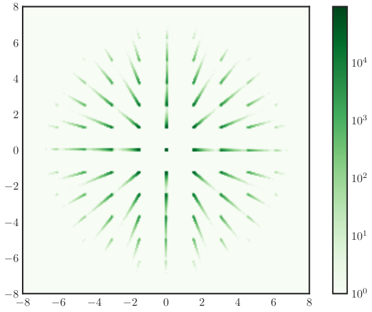
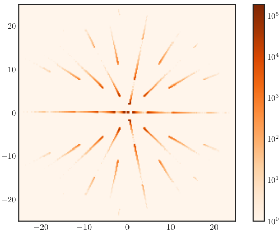
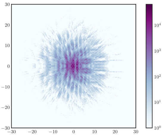
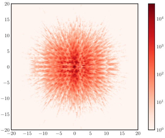
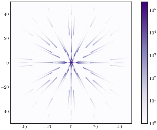
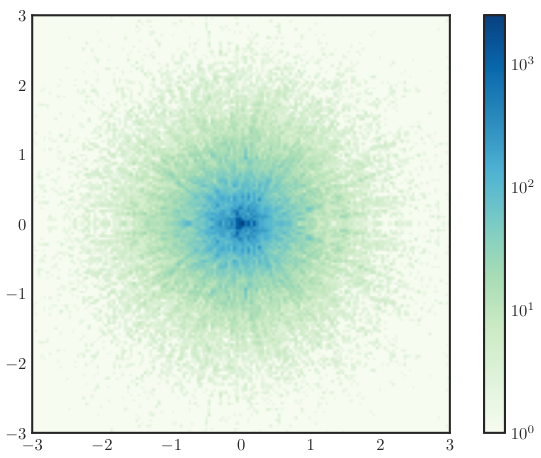
Computer programs such as SAGE has good algorithms which uses Farey symbols to find generators for congruence groups and to solve the the word problem in this context. These are based on [46] (See also [47]). Using the above techniques we plot various histograms of $(\frac{\hbox{vol}\left({\Gamma\backslash\mathbb{H}}\right)}{4\log(c^{2})})^{l/2}(2\pi i)^{l}I_{i\infty}^{a/c}(v)$ with logarithmic colorgrading. For the first 5 plots we use $q=37$ and $M=20000$ , which gives about 3 million datapoints. For the final plot we have used $q=41$ and $M=5500$ which gives about $2.2\cdot 10^{5}$ datapoints. In all the plots we observe the radial symmetry predicted by Theorem 6.1.

Acknowledgments

We are grateful to Christian Berg for many useful comments on Section 5, and to Wadim Zudilin, Christian Krattenthaler and Guoniu Han for discussions and correspondence that led to (160).

References

[1] Peter Banks, Erik Panzer, and Brent Pym, Multiple zeta values in deformation quantization, Inventiones mathematicae 222 (2020), no. 1, 79–159.
[2] Christian Berg, The Cube of a Normal Distribution is Indeterminate, The Annals of Probability 16 (1988), no. 2, 910–913.
[3] Christian Berg and Marco Thill, Rotation invariant moment problems, Acta Mathematica 167 (1991), 207–227.
[4] Sandro Bettin, High moments of the Estermann function, Algebra & Number Theory 13 (2019), no. 2, 251–300.
[5] Sandro Bettin and Sary Drappeau, Limit laws for rational continued fractions and value distribution of quantum modular forms, arXiv:1903.00457 (2019), 42 pp.
[6] Patrick Billingsley, Probability and measure, third ed., Wiley Series in Probability and Mathematical Statistics, John Wiley & Sons Inc., New York, 1995. MR 1324786
[7] by same author, Convergence of probability measures, second ed., Wiley Series in Probability and Statistics: Probability and Statistics, John Wiley & Sons, Inc., New York, 1999. MR 1700749
[8] B. J. Birch, Elliptic curves over $Q$ : A progress report, 1969 Number Theory Institute (Proc. Sympos. Pure Math., Vol. XX, State Univ. New York, Stony Brook, N.Y., 1969), Amer. Math. Soc., Providence, R.I., 1971, pp. 396–400. MR 0314845
[9] Christian Bogner and Francis Brown, Feynman integrals and iterated integrals on moduli spaces of curves of genus zero, Communications in Number Theory and Physics 9 (2015), no. 1, 189–238. MR 3339854
[10] Francis Brown, Mixed Tate motives over $\mathbb{Z}$ , Annals of Mathematics. Second Series 175 (2012), no. 2, 949–976. MR 2993755
[11] by same author, From the Deligne-Ihara conjecture to multiple modular values, Profinite Monodromy, Galois Representations, and Complex Functions (Masanobu Kaneko, ed.), vol. 2120, RIMS Kôkyûroku, 2019, p. 25.
[12] by same author, A multi-variable version of the completed Riemann zeta function and other $L$ -functions, Profinite Monodromy, Galois Representations, and Complex Functions (Masanobu Kaneko, ed.), vol. 2120, RIMS Kôkyûroku,, 2019, p. 27.
[13] Roelof Bruggeman and Youngju Choie, Multiple period integrals and cohomology, Algebra & Number Theory 10 (2016), no. 3, 645–664. MR 3513133
[14] Roelof Bruggeman and Nikolaos Diamantis, Fourier coefficients of Eisenstein series formed with modular symbols and their spectral decomposition, J. Number Theory 167 (2016), 317–335. MR 3504050
[15] Daniel Bump, Automorphic forms and representations, Cambridge Studies in Advanced Mathematics, vol. 55, Cambridge University Press, Cambridge, 1997. MR 1431508
[16] Kuo-Tsai Chen, Iterated path integrals and generalized paths, Bulletin of the American Mathematical Society 73 (1967), 935–938. MR 217717
[17] by same author, Algebras of iterated path integrals and fundamental groups, Transactions of the American Mathematical Society 156 (1971), 359–379. MR 275312
[18] by same author, Iterated Integrals of Differential Forms and Loop Space Homology, Annals of Mathematics 97 (1973), no. 2, 217–246.
[19] by same author, Iterated path integrals, Bulletin of the American Mathematical Society 83 (1977), no. 5, 831–879. MR 454968
[20] Gautam Chinta, Nikolaos Diamantis, and Cormac O’Sullivan, Second order modular forms, Acta Arith. 103 (2002), no. 3, 209–223. MR 1905087
[21] Gautam Chinta, Ivan Horozov, and Cormac O’Sullivan, Noncommutative modular symbols and Eisenstein series, Automorphic Forms and Related Topics (Providence, Rhode Island) (Samuele Anni, Jay Jorgenson, Lejla Smajlović, and Lynne Walling, eds.), Contemporary Mathematics, vol. 732, American Mathematical Society, June 2019, pp. 27–45.
[22] YoungJu Choie, Parabolic cohomology and multiple Hecke L-values, The Ramanujan Journal 41 (2016), no. 1, 543–561.
[23] YoungJu Choie and Nikolaos Diamantis, Rankin-Cohen brackets on higher order modular forms, Multiple Dirichlet Series, Automorphic Forms, and Analytic Number Theory, Proc. Sympos. Pure Math., vol. 75, Amer. Math. Soc., Providence, RI, 2006, pp. 193–201. MR 2279937
[24] YoungJu Choie and Kentaro Ihara, Iterated period integrals and multiple Hecke $L$ -functions, Manuscripta Mathematica 142 (2013), no. 1-2, 245–255. MR 3081007
[25] YoungJu Choie and Kohji Matsumoto, Functional equations for double series of Euler type with coefficients, Advances in Mathematics 292 (2016), 529–557. MR 3464029
[26] Petru Constantinescu, Distribution of modular symbols in $\mathbb{H}^{3}$ , International Mathematics Research Notices (2020), rnaa241.
[27] John E. Cremona, Algorithms for modular elliptic curves, second ed., Cambridge University Press, Cambridge, 1997. MR 1628193 (99e:11068)
[28] Anton Deitmar and Ivan Horozov, Iterated Integrals and Higher Order Invariants, Canadian Journal of Mathematics 65 (2013), no. 3, 544–552.
[29] Pierre Deligne and Alexander B. Goncharov, Groupes fondamentaux motiviques de Tate mixte, Annales scientifiques de l’École Normale Supérieure 38 (2005), no. 1, 1–56.
[30] Nikolaos Diamantis and David Sim, The classification of higher-order cusp forms, J. Reine Angew. Math. 622 (2008), 121–153. MR 2433614
[31] Sary Drappeau and Asbjørn Christian Nordentoft, Central values of additive twists of Maass forms $L$ -functions, arXiv:2208.14346, August 2022.
[32] William Duke, John B. Friedlander, and Henryk Iwaniec, The subconvexity problem for Artin L-functions, Invent. Math. 149 (2002), no. 3, 489–577. MR 1923476
[33] John D. Fay, Fourier coefficients of the resolvent for a Fuchsian group, J. Reine Angew. Math. 293/294 (1977), 143–203. MR 0506038
[34] Jean Françon and Gérard Viennot, Permutations selon leurs pics, creux, doubles montées et double descentes, nombres d’Euler et nombres de Genocchi, Discrete Mathematics 28 (1979), no. 1, 21–35. MR 542933
[35] José Ignacio Burgos Gil and Javier Fresán, Multiple zeta values: From numbers to motives, Clay Mathematics Proceedings, to appear (2017), 379.
[36] Dorian Goldfeld, The distribution of modular symbols, Number Theory in Progress, Vol. 2 (Zakopane-Kościelisko, 1997), de Gruyter, Berlin, 1999, pp. 849–865. MR 2000g:11040
[37] by same author, Zeta functions formed with modular symbols, Automorphic Forms, Automorphic Representations, and Arithmetic (Fort Worth, TX, 1996), Proc. Sympos. Pure Math., vol. 66, Amer. Math. Soc., Providence, RI, 1999, pp. 111–121. MR 2000g:11039
[38] Richards Hain, The Hodge de Rham theory of relative Malcev completion, Annales Scientifiques de l’École Normale Supérieure 31 (1998), no. 1, 47–92.
[39] Kentaro Ihara and Takashi Takamuki, The quantum ${\mathfrak{g}}_{2}$ invariant and relations of multiple zeta values, Journal of Knot Theory and Its Ramifications 10 (2001), no. 07, 983–997.
[40] Henryk Iwaniec, Spectral methods of automorphic forms, second ed., Graduate Studies in Mathematics, vol. 53, American Mathematical Society, Providence, RI, 2002. MR 1942691
[41] Henryk Iwaniec and Emmanuel Kowalski, Analytic number theory, American Mathematical Society Colloquium Publications, vol. 53, American Mathematical Society, Providence, RI, 2004. MR 2061214
[42] Jay Jorgenson and Cormac O’Sullivan, Unipotent vector bundles and higher-order non-holomorphic Eisenstein series, J. Théor. Nombres Bordeaux 20 (2008), no. 1, 131–163. MR 2434161
[43] Peter Kleban and Don Zagier, Crossing probabilities and modular forms, J. Statist. Phys. 113 (2003), no. 3-4, 431–454. MR 2013692
[44] Christian Kleiber and Jordan Stoyanov, Multivariate distributions and the moment problem, Journal of Multivariate Analysis 113 (2013), 7–18.
[45] Maxim Kontsevich, Operads and Motives in Deformation Quantization, Letters in Mathematical Physics 48 (1999), no. 1, 35–72.
[46] Ravi S. Kulkarni, An Arithmetic-Geometric Method in the Study of the Subgroups of the Modular Group, American Journal of Mathematics 113 (1991), no. 6, 1053.
[47] Chris A. Kurth and Ling Long, Computations with finite index subgroups of $PSL_{2}(\mathbb{Z})$ using Farey Symbols, Advances in Algebra and Combinatorics, World Scientific, June 2008, pp. 225–242.
[48] Thang Tu Quoc Le and Jun Murakami, Kontsevich’s integral for the Kauffman polynomial, Nagoya Mathematical Journal 142 (1996), no. none, 39–65.
[49] Tu Quoc Thang Le and Jun Murakami, Kontsevich’s integral for the Homfly polynomial and relations between values of multiple zeta functions, Topology and its Applications 62 (1995), no. 2, 193–206.
[50] Jungwon Lee and Hae-Sang Sun, Dynamics of continued fractions and distribution of modular symbols, arXiv:1902.06277 (2019), 42 pp.
[51] Michel Loève, Probability theory. I, fourth ed., Graduate Texts in Mathematics, vol. 45, Springer-Verlag, New York, 1977. MR 0651017
[52] Hans Maass, Über eine neue Art von nichtanalytischen automorphen Funktionen und die Bestimmung Dirichletscher Reihen durch Funktionalgleichungen, Math. Ann. 121 (1949), 141–183. MR 0031519
[53] Ju. I. Manin, Parabolic points and zeta functions of modular curves, Izv. Akad. Nauk SSSR Ser. Mat. 36 (1972), 19–66. MR 0314846
[54] Yuri I. Manin, Iterated Shimura integrals, Mosc. Math. J. 5 (2005), no. 4, 869–881, 973. MR 2266463
[55] by same author, Iterated integrals of modular forms and noncommutative modular symbols, Algebraic Geometry and Number Theory, Progr. Math., vol. 253, Birkhäuser Boston, Boston, MA, 2006, pp. 565–597. MR 2263200
[56] by same author, Lectures on modular symbols, Arithmetic Geometry, Clay Math. Proc., vol. 8, Amer. Math. Soc., Providence, RI, 2009, pp. 137–152. MR 2498060
[57] Barry Mazur, Courbes elliptiques et symboles modulaires, (1973), 277–294. Lecture Notes in Math., Vol. 317. MR 0429921
[58] Barry Mazur and Karl Rubin, Arithmetic Conjectures Suggested by the Statistical Behavior of Modular Symbols, Experimental Mathematics 0 (2021), no. 0, 1–16.
[59] Philippe Michel, Analytic number theory and families of automorphic L-functions, Automorphic Forms and Applications, IAS/Park City Math. Ser., vol. 12, Amer. Math. Soc., Providence, RI, 2007, pp. 181–295. MR 2331346
[60] Saralees Nadarajah, The Kotz-type distribution with applications, Statistics 37 (2003), no. 4, 341–358.
[61] Asbjørn Christian Nordentoft, Central values of additive twists of modular $L$ -functions, arXiv:1812.08378 (2018), 1–40.
[62] by same author, Central values of additive twists of cuspidal $L$ -functions, Journal für die Reine und Angewandte Mathematik. 776 (2021), 255–293. MR 4279108
[63] Cormac O’Sullivan, Properties of Eisenstein series formed with modular symbols, J. Reine Angew. Math. 518 (2000), 163–186. MR 2000j:11073
[64] Yiannis N. Petridis, Spectral deformations and Eisenstein series associated with modular symbols, Int. Math. Res. Not. (2002), no. 19, 991–1006. MR 1 903 327
[65] Yiannis N. Petridis and Morten S. Risager, Modular symbols have a normal distribution, Geom. Funct. Anal. 14 (2004), no. 5, 1013–1043. MR 2105951
[66] by same author, Arithmetic statistics of modular symbols, Inventiones mathematicae 212 (2018), no. 3, 997–1053. MR 3802302
[67] Christophe Reutenauer, Free Lie algebras, London Mathematical Society Monographs. New Series, vol. 7, The Clarendon Press, Oxford University Press, New York, 1993. MR 1231799
[68] Walter Roelcke, Das Eigenwertproblem der automorphen Formen in der hyperbolischen Ebene. I, II., (1966).
[69] Atle Selberg, Harmonic analysis and discontinuous groups in weakly symmetric Riemannian spaces with applications to Dirichlet series, J. Indian Math. Soc. (N.S.) 20 (1956), 47–87. MR 0088511
[70] by same author, On the estimation of Fourier coefficients of modular forms, Proc. Sympos. Pure Math., Vol. VIII, Amer. Math. Soc., Providence, R.I., 1965, pp. 1–15. MR 0182610
[71] Michel Waldschmidt, Multiple polylogarithms: An introduction, Number Theory and Discrete Mathematics (Chandigarh, 2000), Trends Math., Birkhäuser, Basel, 2002, pp. 1–12. MR 1952273
[72] Matthew P. Young, Explicit calculations with Eisenstein series, Journal of Number Theory 199 (2019), 1–48.

The distribution of Manin’s iterated integrals of modular forms.Thanks: The research of Nils Matthes was supported by a Walter Benjamin Fellowship of the DFG.The research of Morten S. Risager was supported by the Grant DFF-7014-00060B from Independent Research Fund Denmark

Abstract.

2020 Mathematics Subject Classification

1. Introduction

Theorem 1.1.

Theorem 1.2.

Theorem 1.3.

Remark 1.

Remark 2.

Remark 3.

Remark 4.

Remark 5.

2. Manin’s noncommutative modular symbols

Proposition 2.1.

3. Eisenstein series twisted with noncommutative modular symbols

Remark 6.

Remark 7.

3.1. The Laplacian

3.2. Taking derivatives

Proposition 3.1.

Proof.

Corollary 3.2.

3.3. Meromorphic continuation of the automorphic twisted Eisenstein series

Theorem 3.3.

Sketch of proof.

Proposition 3.4.

Proof.

Proposition 3.5.

Proof.

Theorem 3.6.

Proof.

Theorem 3.7.

Proof.

Theorem 3.8.

3.4. Fourier coefficients of higher order twisted Eisenstein series

Proposition 3.9.

Proof.

Theorem 3.10.

Proof.

Remark 8.

Remark 9.

4. Moments of noncommutative modular symbols

Theorem 4.1.

Remark 10.

Theorem 4.2.

Proof.

Theorem 4.3.

Proof.

5. Limits of complex random variables

Theorem 5.1.

Proof.

Remark 11.

Remark 12.

Remark 13.

6. Distributions of noncommutative modular symbols

Theorem 6.1.

Proof.

Remark 14.

Remark 15.

Example 6.2.

7. Special values of multiple LL-functions

7.1. Continuation and functional equation of multiple LL-functions

Theorem 7.1.

7.2. Additive twists of multiple LL-functions.

Theorem 7.2.

Remark 16.

8. Numerics

Acknowledgments

References

7. Special values of multiple $L$ -functions

7.1. Continuation and functional equation of multiple $L$ -functions

7.2. Additive twists of multiple $L$ -functions.