Density Functional Theory for Electronic Excited States
Abstract
This chapter provides a basic introduction to excited-state extensions of density functional theory (DFT), including time-dependent (TD-)DFT in both its linear-response and its explicitly time-dependent formulations. As applied to the Kohn-Sham DFT ground state, linear-response theory affords an eigenvalue-type problem for the excitation energies in a basis of singly-excited Slater determinants, and is widely known simply as “TDDFT” despite its frequency-domain formulation. This form of TDDFT is the mostly widely-used quantum-chemical method for excited states, due to a favorable combination of low cost and reasonable accuracy. The chapter surveys the accuracy of linear-response TDDFT, which is generally more sensitive to the details of the exchange-correlation functional as compared to ground-state DFT, and also describes some known systemic problems exhibited by this approach. Some of those problems can be corrected on a case-by-case basis using orbital-optimized, excited-state self-consistent field (SCF) calculations, in what is known as excited-state Kohn-Sham theory or a “SCF” procedure, a class of methods that includes restricted open-shell Kohn-Sham theory. Recent successes of these approaches are highlighted, including double excitations and core-level excitations. Finally, explicitly time-dependent (or “real-time”) TDDFT involves propagation of the molecular orbitals in time following an external perturbation, according to the Kohn-Sham analogue of the time-dependent Schrödinger equation. The time-dependent approach has been used to model strong-field electron dynamics, and in the weak-field limit it provides a route to broadband spectra based on the time evolution of the dipole moment function. This is useful for describing high-energy excitations (as in x-ray spectroscopy) and in systems where the density of states is high, as demonstrated by a few examples.
1 Overview
Following its implementation in molecular quantum chemistry codes in the early 1990s,1, 2, 3, 4, 5, 6 density functional theory (DFT) quickly emerged as the most popular tool for ground-state electronic structure calculations due to its favorable balance of relatively low cost with reasonable accuracy for thermochemistry. The first excited-state implementations quickly followed,7, 8, 9, 10, 11, 12 based on a linear-response (LR) formalism13, 14, 15 that mirrors much earlier work on time-dependent Hartree-Fock theory.16 (The historical development of TDDFT has been summarized elsewhere.17) The LR formulation is now known almost universally as “time-dependent” (TD-)DFT, despite its frequency-domain formulation and implementation. In its most pedestrian applications, LR-TDDFT produces vertical excitation energies for closed-shell molecules at ground-state geometries to within a statistical accuracy of eV,18 at a cost that is often only a few times more than the cost of the ground-state self-consistent field (SCF) calculation and possessing the same formal scaling.19 This is a useful accuracy for electronic absorption spectra. In view of its low cost, LR-TDDFT has therefore become the de facto method for computing electronic excitation spectra of finite molecular systems, although some fundamental problems remain in its application to periodic materials.20, 21, 22 LR-TDDFT is also becoming increasingly popular for photochemical applications,23, 24, 25 despite some problems with the description of conical intersections.26, 27, 28 In part, this popularity is due to a growing recognition that complete active-space (CAS-)SCF methods cannot be considered quantitative approaches for excited-state dynamics,29, 30, 31, 32 due to a lack of dynamical electron correlation effects.
This chapter provides an overview of TDDFT and other DFT-based methods for computing excitation spectra, excited-state properties, and for simulating photochemical reactions, emphasizing theory rather than applications but with some molecular examples to motivate the discussion. For those unfamiliar with the formal underpinnings of TDDFT, a natural question to ask is “what does time have to do with excitation energies?” In fact, one knows from basic quantum mechanics that the time evolution of a non-stationary wave function encodes the system’s excitation energies via the Bohr frequencies, , therefore in principle the time evolution of a quantum system can be used to extract excitation energies. The existence of a time-dependent extension of DFT is formally justified by the Runge-Gross theorem,33, 34, 35, 36, 37, 38, 39 which provides something akin to a time-dependent extension of the first Hohenberg-Kohn theorem for the ground state,40 i.e., a density-to-potential mapping. In the time-dependent case there are important caveats about initial-state dependence and memory effects.41, 42, 43 Those issues have yet to be fully resolved in a computationally feasible way, but this has not stymied the practical development and application of TDDFT.
Following a perturbation to the ground state, which creates a superposition of energy eigenstates, the Fourier components of the time-dependent dipole moment are precisely the Bohr frequencies. A Fourier transform of the dipole moment function is itself an absorption spectrum,44
| (1) |
Excitation energies are also encoded in the isotropic frequency-dependent polarizability, , which has a sum-over-states expression
| (2) |
where is the electron mass, , and
| (3) |
is the dimensionless dipole oscillator strength for the transition.44 The poles of response function therefore encode excitation energies, with residues that encode oscillator strengths.19 In the early days of quantum chemistry, Eq. (2) was actually used to compute excitation energies for atoms and atomic ions,45, 46 by computing as the response to an applied field, and a version of this approach would eventually reappear in the form of “real-time” TDDFT.47, 48 The poles of the Kohn-Sham response function also serve this purpose,49, 9, 50 and the LR formalism applied to the Kohn-Sham ground state turns this idea into a robust computational paradigm, in the form of an eigenvalue-type problem for the excitation energies.13, 14, 15 Although the LR formulation exists strictly in the frequency or energy domain, the time-dependent origins of the phenomenology have persisted in the name “TDDFT”.
Despite its overwhelming popularity, LR-TDDFT excitation energies do tend to be more sensitive to the details of the exchange-correlation (XC) functional as compared to ground-state properties computed with DFT. In some sense, the statistical accuracy of eV that is quoted above should therefore be interpreted as representative of the best-case scenario with state-of-the-art functionals, and assuming that certain systemic pathologies can be avoided. LR-TDDFT may not be the theory that we want, but it remains the best theory that we have for excited states of large and even medium-size molecules. This theory is introduced formally in Section 2 and that discussion constitutes the most substantial part of this chapter, just as LR-TDDFT occupies the most significant place amongst excited-state DFT methods. It holds that position because it is easy to use, not significantly more expensive than ground-state DFT, and provides a slew of excited states in an automated way, starting from a ground-state SCF solution.
While the accuracy of LR-TDDFT is often quite reasonable, certain systemic problems have been identified and excited-state Kohn-Sham procedures have been developed to circumvent these. Rather than applying LR to the ground state, these methods look for an excited-state (non-aufbau) solution to the SCF equations, and for this reason the excited-state Kohn-Sham approach is often called a “SCF” method. Although not formally justified by the Runge-Gross theorem, the SCF approach has an admirable record of rectifying the deficiencies of LR-TDDFT, again at a cost comparable to that of a ground-state DFT calculation. What is lost in the SCF approach is the ability to compute a whole spectrum of states at once, making the state-specific SCF procedure much more labor-intensive for the user. This approach is described in Section 3.
Finally, it is possible to take the time dependence in TDDFT at face value and to propagate Kohn-Sham molecular orbitals (MOs) in time, following a perturbation applied to the ground-state density. This is accomplished by solving the time-dependent Kohn-Sham (TDKS) equation,
| (4) |
which is a one-electron analogue of the time-dependent Schrödinger equation. (Here, is a spin index.) The one-electron effective Hamiltonian in Eq. (4) is the Fock operator that comes from the ground-state Kohn-Sham eigenvalue problem that determines the MOs:
| (5) |
The “real-time” approach to TDDFT,51, 52 which is described in Section 4, consists in solving Eq. (4) by propagating the MOs in time following a perturbation to the ground-state that creates a time-evolving density,
| (6) |
expressed here for -spin electrons. (The total charge density is .) This approach can be used to simulate strong-field electron dynamics,53 which is a topic of contemporary interest in attosecond molecular science.54, 55, 56, 57 It also provides a route to broadband spectra via Fourier transform of the time-dependent dipole moment function, in a direct realization of Eq. (1).
This chapter assumes a basis familiarity with ground-state DFT, as represented by the SCF eigenvalue problem in Eq. (5), which will serve as our starting point. It should therefore be familiar that the Fock operator takes the form
| (7) |
in atomic units. The quantities , , and are known as the external, Hartree, and XC potentials, respectively. In the field-free case, the external potential is simply the interaction of the electrons with the nuclei,58
| (8) |
More generally, might also contain a field-dependent contribution such as in the presence of an electric field . The Hartree (or Coulomb) potential describes self-repulsion of the electrons,58 equivalent to what is often called “” in Hartree-Fock theory.59, 40 It is a functional of the density, given by
| (9) |
The final component of is , the XC operator for -spin electrons. In “pure” Kohn-Sham theory, this quantity should be a local potential rather than an operator, but herein we allow the possibility for mixing some nonlocal Hartree-Fock exchange (HFX), as is done in the hybrid density functionals that are most useful in molecular DFT. For hybrid functionals is a nonlocal operator and this scenario is sometimes called generalized Kohn-Sham theory,39 although the use of hybrid functionals can no longer be considered exotic in molecular DFT.
The textbook by Koch and Holthausen40 is a good resource for ground-state DFT (though not for TDDFT), as are several literature overviews.60, 58 Updated ground-state benchmarks, relative to the rather dated ones in Ref. 40, can be found elsewhere.61, 62 For TDDFT, the textbook by Ullrich,63 or else overviews by Gross and co-workers,64, 65, 36 provide the rigorous foundations of the theory, which are mostly omitted here. Several other reviews cover LR-TDDFT in a pedagogical way.66, 67, 68 For overviews of molecular applications of LR-TDDFT, see reviews by Jacquemin and co-workers,69, 70, 71, 72, 73 who have also reviewed the accuracy benchmarks18 and functional selection.74
2 Linear-Response (“Time-Dependent”) DFT
This section describes the formalism and application of LR-TDDFT, commonly known simply as “TDDFT”. The starting point is the TDKS equation [Eq. (4)] that describes how the ground-state MOs evolve in time following a perturbation that is applied at . If that perturbation is taken to be a time-oscillating field at frequency ,
| (10) |
then in the weak-field limit (), the response of the ground state can be computed exactly using first-order perturbation theory.15 Formally, one ought to show that the poles of the frequency-dependent response function can be obtained from those of the independent-particle (Kohn-Sham) response function,9 but for that exercise the reader is referred to reviews by Marques and Gross.64, 65 For a derivation of LR-TDDFT based on a variational principle, see Ref. 75.
2.1 Theoretical Formalism
The derivation from perturbation theory starts from the equivalent Liouville-von Neumann (LvN) form of the TDKS equation, which is
| (11) |
where
| (12) |
is the time-evolving one-electron density operator for -spin electrons. Expanding Eq. (11) to first order in the perturbed Fock and density matrices, in the presence of the perturbation , one obtains the unperturbed LvN equation at zeroth order. This is equivalent to the ground-state Kohn-Sham eigenvalue problem in Eq. (5). Working equations for LR-TDDFT are obtained by equating the first-order terms,11, 15, 66 as elaborated below.
2.1.1 Linear Response Theory
To consider this in more detail, recognize that the perturbation in Eq. (10) is a one-electron operator whose spatial part can be expanded in the MO basis, leaving the time dependence to be carried by . Introducing a set of unknown coefficients and , representing real and imaginary parts of the first-order response, the first-order perturbed density matrix can be expressed as
| (13) |
where is the unperturbed density matrix at . This change in the density matrix is accompanied by a corresponding change in the Fock matrix. Through first order, the Fock matrix is11
| (14) |
where the unperturbed Fock operator has the form given in Eq. (7). The first-order response of the density matrix is thus coupled to a term of the form11
| (15) |
The first term, , is a Coulomb integral expressed in Mulliken notation,59 while . The latter quantity is discussed in more detail below.
So far, the MO indices are arbitrary and could refer either to occupied or virtual orbitals. In fact, the idempotency condition imposes restrictions. Through first order, the idempotency condition is
| (16) |
since . As a matrix, contains only occupied–occupied and virtual–virtual blocks because the occupied–virtual block vanishes as a condition of SCF convergence.76 Using to index occupied MOs and for virtual MOs, this means , so the constraint in Eq. (16) implies that the only non-vanishing coefficients in are and .11, 66 Conventional LR-TDDFT notation is obtained by relabeling these coefficients as
| (17a) | ||||
| (17b) | ||||
Collecting these unknowns into vectors and , one may rewrite the first-order terms in the LvN equation in matrix form as66, 67, 68
| (18) |
This represents a system of equations for the excitation energies and the amplitudes and , and constitutes the basic working equations of LR-TDDFT. (The index , which counts excited states, will usually be omitted for compactness.) The system in Eq. (18) is often called the Casida equations,13, 14 although these are formally identical to the equations of time-dependent Hartree-Fock theory.16 The matrices and are known as orbital Hessians,19 for reasons that are discussed below, and they derive from the derivative of with respect to in Eq. (15). In the canonical MO basis, the matrix elements of and are66, 19
| (19a) | ||||
| (19b) | ||||
where . The quantity will be used throughout this chapter to mean the coefficient of HFX (often called “exact exchange”) contained in the functional , with . For example, for B3LYP, meaning meaning 20% HFX and 80% semilocal exchange. We have chosen to separate the HFX terms in Eq. (19), which can be expressed in terms of electron repulsion integrals and , leaving as the second functional derivative of the semilocal contribution, .
The solution of Eq. (18) parameterizes the transition density matrix for the excitation in question. In real space, this quantity is10, 15, 19
| (20) |
The unknowns and satisfy a bi-orthogonal normalization condition,15
| (21) |
which is also a feature of the much older time-dependent Hartree-Fock (TDHF) theory.16 For historical reasons, TDHF is also known as the random phase approximation (RPA),77, 78 because it can be derived within an equation-of-motion formalism for the single-particle excitation operators,68 similar to the historical RPA.77 However, TDHF/RPA can also be considered to be a special case of LR-TDDFT corresponding to the Hartree-Fock functional, i.e., and .
The number of unknown amplitudes in Eq. (18) is , hence to solve this equation for all of the excitation energies would incur sixth-order cost, . Because matrix–vector products such as or can be computed with only fourth-order cost, in practical calculations Eq. (18) is solved iteratively for just the lowest few eigenvalues ().79, 7, 10, 80, 81, 82 The cost of that calculation scales as ,19 which is typically not significantly greater than the cost of the ground-state SCF calculation if . Therefore if ground-state DFT is feasible then LR-TDDFT is probably tractable also, at least for the lowest few excited states. It is worth noting, however, that the memory footprint to solve Eq. (18) is , which is significantly more than the ground-state memory requirement. This can become a problem for large systems if a large number of excited states is desired, e.g., in models of semiconductors where a band structure is emerging.83 For such applications, the real-time approach that is described in Section 4 offers a low-memory alternative to LR-TDDFT.
Some alternative forms of the basic LR-TDDFT equation are also worth considering. We first note that the matrices and in Eq. (19) can be rewritten as
| (22a) | ||||
| (22b) | ||||
where is a coupling matrix,13, 84
| (23) |
with a Hartree–XC kernel.67 In practice, this looks like the energy-transfer coupling85 between transition densities and . One can therefore consider that solution of the LR equations reveals how the zeroth-order, independent-particle excitations are coupled to obtain excited states of the interacting system.
Assuming that the orbitals are real, so that and , then Eq. (18) is equivalent to a pair of equations
| (24) |
which makes it clear that Eq. (18) is not a conventional eigenvalue problem. However, upon introducing new variables
| (25) |
which satisfy the more conventional normalization condition ,86, 87 the LR-TDDFT equations can be transformed into either of two equivalent, Hermitian eigenvalue problems.88, 89, 86, 87, 81 These are
| (26) |
where
| (27) |
The version of Eq. (26) is especially convenient for semilocal functionals (), because in that case is diagonal and one obtains a Hermitian eigenvalue problem with half the dimension of the original pseudo-eigenvalue problem in Eq. (18).
For a closed-shell (spin-restricted) ground state, another important transformation is
| (28a) | ||||
| (28b) | ||||
which affords amplitudes for singlet () and triplet () spin functions. Making use of the unitary transformation78
| (29) |
in addition to Eq. (28), one obtains singlet and triplet versions of that function as stability matrices.7, 8, 86 In other words, these are Hessian matrices whose eigenvalues characterize whether the ground state is stable with respect to orbital rotations. For example, the singlet stability matrix is86
| (30) |
A negative eigenvalue in indicates an instability, which looks like a negative excitation energy from the standpoint of LR-TDDFT. This correspondence is a consequence of the Thouless theorem,90 which states that orbital rotations (and therefore orbital relaxation) can always be parameterized as single excitations. Along similar lines, eigenvalues of the triplet instability matrix86
| (31) |
indicate whether the ground-state solution is stable with respect to spin symmetry breaking (restricted unrestricted).91 In the presence of an unstable reference state, the transformation in Eq. (25) may become problematic, which can lead to failure of certain iterative LR-TDDFT algorithms.
2.1.2 Adiabatic Approximation
We have not yet discussed the key ingredient in the orbital Hessian matrices that makes LR-TDDFT different from TDHF/RPA, namely, the exchange-correlation kernel, . A more careful application of LR theory would note that the quantities and are themselves functions of the excitation energy .13, 14, 15 In wave function terms, this can be understood based on the fact that any exact theory of many-electron excitation energies that is formulated as an effective single-particle theory must ultimately invoke an effective Hamiltonian that is energy-dependent, in order to encapsulate the effects of higher-order excitations.14, 92, 93 (In many-body theory this energy-dependent contribution is sometimes called the “self-energy”.94) Proof-of-concept models for an energy-dependent kernel have been put forward,95, 42, 43, 93 which have close connections to many-body perturbation theory and the Bethe-Salpeter equation.92, 93 However, there are no production models for molecular Hamiltonians at present.
To appreciate the nature of the approximation in neglecting the energy dependence of , consider that this quantity arises in Eq. (15) as the second functional derivative of the XC energy with respect to the density, or the first derivative of the XC potential. For a time-evolving density , this means41
| (32) |
(This expression leaves in the form of an operator, which technically makes this an example of generalized Kohn-Sham theory.39) The time dependence in means that this quantity depends on the whole history of the time evolution of the density,41, 42, 43 imparting a frequency dependence upon Fourier transformation: . For practical purposes, it is basically a requirement to invoke the adiabatic approximation,13, 96, 68 which assumes locality in time and therefore differentiates with respect to the instantaneous density:13
| (33) |
The “memory” of the kernel is thereby neglected, tantamount to assuming that can be approximated using a conventional ground-state energy functional , whose functional derivative is evaluated using the time-evolving density:96
| (34) |
Time dependence is thus carried entirely by the density and not by the functional. The frequency dependence of disappears and conventional (ground-state) density functionals are all that is required for LR-TDDFT within the adiabatic approximation.
One immediate ramification of this approximation is that the LR-TDDFT equations have precisely solutions for the excitation energy , coinciding with the number of unknown amplitudes and . In wave function language, these are the “one-particle, one-hole” (1p1h) states, as in conventional configuration interaction with single excitations (CIS). States with significant double-excitation character (2p2h states) are either absent altogether,97, 95, 96, 98, 99 or at best severely shifted.98 The latter are therefore generally considered to be out of reach within the adiabatic approximation that is ubiquitous in practical LR-TDDFT calculations.99
2.1.3 Tamm-Dancoff Approximation
Given a ground-state functional , all that is required for LR-TDDFT within the adiabatic approximation are second functional derivatives
| (35) |
from which the matrix elements of and can be evaluated. Upon solution of Eq. (18) or one of its equivalent forms, it is often found that the amplitudes are – times smaller than the largest . Invoking the approximation , one obtains a conventional Hermitian eigenvalue problem
| (36) |
whose dimension is half that of the original LR-TDDFT pseudo-eigenvalue problem, and where the matrix does not appear. The basis for this approximation can be understood from the fact that the matrix elements of are typically much larger (at least along the diagonal) as compared to the matrix elements of , because the leading contribution to is a difference in one-particle energy levels (). For historical reasons that are related to a similar approximation that is made in nuclear physics,63 neglect of is known as the Tamm-Dancoff approximation (TDA). For hybrid functionals, the reduction in dimension leads to a concomitant reduction in cost although for semilocal functionals the same reduction in dimensionality can be achieved using the version of Eq. (26).
For the Hartree-Fock functional ( and no correlation), Eq. (36) is equivalent to the CIS eigenvalue equation.100 Excited-state wave functions in CIS are linear combinations of singly-excited Slater determinants ,
| (37) |
and for this reason we identify the variables as excitation amplitudes. The neglected amplitudes represent de-excitation, insofar as TDHF/RPA was originally introduced in the nuclear and many-body physics literature as a means to add correlation to the ground state.16, 77 In fact, LR-TDDFT in the form of Eq. (18) was introduced in molecular quantum chemistry as the “DFT random phase approximation”.101, 102 For that reason, solution of Eq. (18) or its equivalents, without invoking the TDA, is sometimes called “RPA”. However, in view of a resurgence of interest in using the RPA formalism as a means for correlating the ground state,103, 104, 105, 106, 107, 108, 109, 110 it is better to refer to Eq. (18) as “full” LR-TDDFT, if there is a need to distinguish it from the TDA version in Eq. (36).
Quantitatively, the impact of the TDA on excitation energies is often eV,11 though a potentially detrimental impact is that oscillator strengths within the TDA no longer satisfy the Thomas-Reiche-Kuhn sum rule,44
| (38) |
This constraint is satisfied by the full LR-TDDFT approach, at least in the complete-basis limit.111, 13, 15 Some small-molecule tests suggest that errors incurred by the TDA are relatively mild (%),112 and perhaps not noticeable in band shapes once vibrational broadening is taken into account.113
A more important consequence of the TDA is that it decouples the excitation energy problem from the ground-state stability problem, whereas for full LR-TDDFT a triplet instability in the ground state manifests as a negative excitation energy, or as an imaginary root of the Hermitian eigenvalue problem in Eq. (26). This may cause problems for eigensolvers that implicitly assume . Note that triplet instabilities are associated with spin-symmetry breaking, i.e., with the emergence of an unrestricted solution that is lower in energy than the restricted solution. Where they appear, these instabilities cause significant artifacts in potential energy surfaces computed using LR-TDDFT, including the appearance of spurious cusps.114, 115, 84, 116, 117 In contrast, the variational nature of the CIS-type equation, as opposed to the pseudo-eigenvalue problem that characterizes full LR-TDDFT, prevents this from happening within the TDA.68
Along similar lines, it has been appreciated for a long time that TDHF specifically is prone to triplet instabilities.90, 118, 119, 91, 120, 121, 122, 123, 124 In fact, the appearance of imaginary excitation energies at equilibrium geometries of small molecules led Furche and Ahlrichs to conclude that this method is “rather useless for the investigation of excited potential energy surfaces”.125 In contrast, spin-symmetry breaking near the equilibrium geometry is often significantly mitigated when DFT is substituted for Hartree-Fock theory.126 Because most molecular LR-TDDFT calculations use hybrid functionals that include some fraction of HFX, it can be expected that problems with triplet instabilities may increase as that fraction increases, which is precisely what is found in practice.127, 128, 129, 130, 131 Similarly, in calculations using range-separated functionals, which incorporate HFX at long range in the electron–electron Coulomb potential, these instabilities are sensitive to the length scale on which that mixing is introduced.132, 133, 134, 135, 136, 137 Invoking the TDA thus improves the accuracy of triplet excitation energies.134, 135, 136 For photochemical problems, where exploration of excited-state potential energy surfaces is paramount, Casida et al. suggest that the TDA is effectively mandatory,138 in order to avoid excitation energies that drop to zero (and then become imaginary) as the system moves through a Coulson-Fischer point where spin-symmetry breaking occurs. Instabilities appear to proliferate as one moves away from the ground-state geometry on an excited potential surface.138, 139, 140 For example, in the photochemical ring-opening reaction of oxirane (C2H4O), 51% of configuration space is estimated to exhibit an instability with semilocal DFT, as compared to 93% of space with B3LYP.138
2.1.4 Analytic Gradients
Photochemical simulations require analytic excited-state gradients. That formalism, which is closely connected to response theory for optical properties,141 is not discussed here but can be found elsewhere.142, 143, 125, 19, 144, 145 Nonadiabatic or “derivative coupling” vectors between excited states,146, 27 which are needed for nonadiabatic molecular dynamics simulations,23, 24, 25, 26, 27 have also been formulated.147, 148, 149, 150, 151, 152, 153, 154 Evaluation of the nonadiabatic couplings has the same formal complexity as evaluation of the excited-state gradient.147, 25
Here, we comment briefly regarding how the gradient formalism bears on static properties of the excited state, such as the dipole moment or atomic population analysis. The density matrix for the excited state can be written
| (39) |
which is sometimes called the “relaxed” density matrix, from which an “unrelaxed” contribution is separated out. Here, represents the ground-state density matrix and the unrelaxed change upon excitation () can be obtained from the amplitudes and . The remaining contribution () represents orbital relaxation.19, 144, 145
The unrelaxed density change can be separated into particle (electron) and hole contributions,
| (40) |
which are given by125, 155, 145, 156
| (41a) | ||||
| (41b) | ||||
These expressions can be rearranged to afford155
| (42a) | ||||
| (42b) | ||||
Note that only contains occupied–occupied () and virtual–virtual () contributions to the excited-state density matrix, not occupied–virtual contributions. The latter are contained in ,125, 19 the evaluation of which requires solution of so-called -vector equations.157 This has the same formal complexity as an excited-state gradient calculation.
Excited-state properties should be computed using the relaxed density matrix , because and make similar contributions.100, 158, 159 Especially when the change in density is large, as for an excitation with significant charge-transfer (CT) character, the use of the unrelaxed density matrix may lead to unacceptable errors in excited-state properties. For example, excited states of -nitroaniline involving intramolecular CT character exhibit relaxed and unrelaxed dipole moments (computed using versus , respectively) that differ by more than 10 D in some cases!158
2.2 Performance and Practice
As discussed above, the formal scaling of LR-TDDFT is for hybrid functionals.19 In practical terms, where only a few low-lying excited states are desired, this means that LR-TDDFT is generally feasible if the corresponding ground-state calculation is practical, perhaps up to about 400 atoms for single-point calculations or 150–250 atoms where excited-state geometry optimization is required,70, 71 with more severe limitations where excited-state frequency calculations are required.160, 71 These estimates are appropriate where basis sets of double- quality are used, which is generally adequate. Triple- basis sets may be considered to be converged.67 Systems that possess a dense manifold of excited states (e.g., semiconductors) can create significant storage bottlenecks for the trial vectors that are required by the iterative eigensolver. In such cases, the “real-time” TDDFT approach of Section 4 may be advantageous, although Section 2.2.1 describes ways to reduce the cost while staying within the confines of LR-TDDFT. Following a discussion of XC functional approximations in Section 2.2.2, the accuracy of LR-TDDFT excitation energies is addressed in Section 2.2.3 by considering its performance for small-molecule benchmarks. Finally, techniques for visualizing and understanding the states that are computed are discussed in Section 2.2.4.
2.2.1 Restriction of the Excitation Manifold
Significant cost reduction in LR-TDDFT calculations for large molecules can be achieved by neglecting some of the amplitudes , in addition to neglecting all of the amplitudes . Figure 1 shows examples of excitation spectra computed for C60 and for , performed by excluding over 70% of the virtual orbitals (based on orbital energies ) without adverse effects on the spectral envelope.161

Similar truncations of the excitation manifold can be used to access core-excited states.162, 163, 164, 165 There is significant interest in core excitations in contemporary quantum chemistry,166, 167, 168, 164, 165, 169 driven by the recent availability of tabletop laser sources with femtosecond time resolution.170, 171, 172, 173, 174 However, core-to-valence excitations lie embedded in an ionization continuum and, at a practical level, lie above all of the valence-excited states, such that the use of iterative eigensolvers is prohibitively expensive if the spectrum must be computed starting from the lowest excitation energies. By retaining only those amplitudes for which is a core orbital on the atom of interest, core-excited states emerge as the smallest eigenvalues and can be computed directly. This “frozen valence occupied” approximation has historically been called “core–valence separation”,175, 176, 177 and it introduced negligible error for K-edge excitations where is a 1s orbital.177 Another strategy to access core-level excitations is energy windowing,178, 162 in which the amplitudes are excluded unless lies within the window of interest.
2.2.2 Exchange-Correlation Functionals
Before considering the accuracy of LR-TDDFT it is useful to introduce a paradigm for classifying various density-functional approximations, for which we use the taxonomy of “Jacob’s ladder”.179, 180, 181 At each rung on this metaphorical ladder, the functional dependence of grows more intricate, incorporating more sophisticated functionality depending on the density, its gradients, the Laplacian, etc.: . In a statistical sense (and only in a statistical sense), it is true that the best functionals on the higher rungs of the ladder outperform the best functionals on the lower rungs.61, 182 These rungs map onto various inputs as follows.
- •
Rung 1: Local Density Approximation (LDA). The baseline LDA functional comes from the uniform electron gas model in which is a functional of only, or of and if the system is spin-polarized. This approach does not afford useful accuracy for molecular quantum chemistry, with errors of 60–100 kcal/mol for atomization energies183, 61 and kcal/mol for barrier heights.61
- •
Rung 2: Generalized Gradient Approximations (GGAs). This class of functionals include a dependence on the density gradients . These are often called “semilocal” approximations, to distinguish them from LDA while acknowledging that in their mathematical form, GGAs remain local in the sense that is a multiplicative potential. GGA functionals significantly improve thermochemistry relative to LDA; typical errors are 10–20 kcal/mol for atomization energies183, 61 and 5–15 kcal/mol for barrier heights.61, 182
- •
Rung 3: Meta-GGAs (mGGAs). These are also semilocal but incorporate additional derivatives including and the kinetic energy density,
(43) The function is related to the electron localization function,184 and together with it can be used to express the noninteracting kinetic energy.185 The best mGGA functionals improve upon GGA thermochemistry, with errors of 5–10 kcal/mol for atomization energies61 and 3–6 kcal/mol for barrier heights.61, 182 It is worth noting that some mGGAs introduce a considerable number of parameters,61 and exhibit basis-set and grid sensitivities suggesting that they may be overfitted.186, 187, 188, 189
- •
Rung 4: Hyper-GGAs. As originally defined by Perdew et al.,179, 180 this category consists of functionals that incorporate “exact exchange and compatible correlation”.179 A few genuine hyper-GGAs have been put forward,190, 191 but it has proven difficult to construct correlation functionals that work well with 100% HFX. As such, the fourth rung on Jacob’s ladder has effectively been redefined to mean hybrid functionals,181 which incorporate some fraction of HFX (), in conjunction with a fraction of semilocal exchange. These functionals are sometimes further categorized as either hybrid GGAs or hybrid mGGAs, depending on the nature of the semilocal contribution. The best hybrid functionals exhibit errors kcal/mol for atomization energies61 and 2–4 kcal/mol in barrier heights.61, 182 This has made hybrids the de facto choice for molecular quantum chemistry.
- •
Rung 5: Double hybrid functionals.192 These incorporate a fraction of the second-order Møller-Plesset (MP2) correlation energy in addition to fractional HFX, which introduces a dependence on the virtual MOs whereas functionals on the lower rungs depend only on the occupied MOs. Although double hybrids exhibit some of the best accuracy in contemporary DFT, with errors of 1–3 kcal/mol for barrier heights,192, 182 the introduction of MP2 correlation brings with it the much slower basis-set convergence of wave function methods, as well as a question of whether the orbital-dependent MP2 term should be self-consistently optimized. (Typically, it is not.192)
A comprehensive list of functionals, up-to-date as of 2017, can be found in Ref. 61. The aforementioned error statistics pertain to ground-state thermochemistry whereas accuracy for vertical excitation energies computed using LR-TDDFT is considered in the next section. For double hybrid functionals, the formulation of LR-TDDFT193 begins to look more like CIS with perturbative double excitations, a method known as CIS(D),194 which incurs a formal scaling of and often requires a form of quasi-degenerate perturbation theory.195, 196 For these reasons, the application of double hybrids to excited-state problems is still in its infancy and is not discussed in this chapter.
In the context of LR-TDDFT there is one further category of functionals that warrants mention, namely, range-separated hybrid (RSH) functionals. These partition the electron–electron Coulomb interaction () into a short-range (SR) component and a long-range (LR) background, typically using the error function (erf):
| (44) |
This partition introduces parameters , , and . The latter is the range separation parameter that determines the length scale () of the separation between the SR and LR components of ; see Fig. 2. Consider a GGA or hybrid functional of the form
| (45) |
where is the semilocal GGA exchange functional and is the coefficient of HFX. The RSH functional corresponding to Eq. (45) is
| (46) |
where
| (47) |
Quantities labeled “SR” or “LR” in these equations are evaluated using the corresponding component of . The idea is to correct the asymptotic behavior of a semilocal potential at long range (using HFX), while attempting to have minimal impact on the SR behavior of the GGA or hybrid GGA in question, since that functional is responsible for the favorable thermochemical predictions in the ground state. RSH functionals have become popular enough that traditional hybrids such as PBE0 or B3LYP are often called “global hybrid” (GH) functionals in contemporary parlance, to emphasize that HFX is added at all length scales in these cases. The definition of in Eq. (47) is consistent with other literature,197, 198, 199 although it is worth noting that this quantity is not truly long-ranged. In fact, the reason that RSH functionals were introduced in the first place is to address the fact that semilocal exchange falls off too rapidly with distance,200, 201, 202 leading to an insufficiently attractive interaction potential between a well-separated electron and hole.203, 201, 202 This is further discussed in Section 2.3.1.
Nomenclature and usage for RSH functionals has become somewhat muddled and the remainder of this section attempts to clarify it. An RSH functional is any that uses a partition of into SR and LR components, with Eq. (44) as the most common partition although other forms have been explored,204, 205, 206, 207, 208, 209 including variants with a three-way partition of into short-, middle-, and long-range contributions.210, 211, 212, 213, 214, 215 For many of these functionals, the range-separation parameter(s) are optimized or fitted alongside other parameters that define the functional and should not be modified. Examples include the “B97” class of functionals216, 217, 218, 219, 220 and range-separated versions of the “Minnesota” functionals.221, 222, 223, 224 These functionals do not always afford correct the asymptotic behavior of the XC potential, however. For the ansatz in Eq. (44), the proper behavior requires but that constraint is sometimes violated (in particular, by the popular CAM-B3LYP functional225) in the interest of obtaining more accurate excitation energies for localized transitions.
In contrast to this empirical approach to range separation, long-range corrected (LRC) functionals represent a subset of RSH functionals that are constrained to include 100% HFX in the limit .200, 226, 227, 228 For a given GGA () or hybrid GGA () functional, the corresponding LRC functional is
| (48) |
The parameter in Eq. (44) still controls the length scale on which LR-HFX is activated, but by construction and therefore for any . The LRC strategy is thus to graft correct asymptotic behavior onto an existing semilocal XC functional, while doing the least possible damage to that functional at short range. Non-empirical adjustment (or “tuning”) of the parameter is often employed in this context, especially where CT states are involved, and this is discussed in Section 2.3.1.
LRC functionals require modification of the semilocal GGA exchange functional in order to use an attenuated Coulomb potential. (HFX integrals can be modified once and for all to separate them into LR and SR contributions.229) There are several routes to modify . The first of these, originally introduced by Hirao and co-workers,200, 201, 202 modifies the exchange inhomogeneity factor that multiplies the electron-gas exchange energy density. This author has suggested that these functionals should be denoted LRC-GGA,230, 231 where “GGA” indicates the semilocal parent functional, e.g., GGA = BLYP or PBE. Note that “LC” is another common abbreviation for long-range correction so that functionals such as LC-BLYP200 might more descriptively be called LRC-BLYP, in order to emphasize which SR-GGA exchange function (BLYP) is being used.
For semilocal exchange functional such as PBE that are based on a model for the exchange hole,232, 233 an alternative strategy is to combine that model with an attenuated Coulomb potential in order to obtain .233, 228 To distinguish this from the LRC-PBE functional constructed using Hirao’s approach, the author has suggested the nomenclature LRC-PBE for the model based on the PBE exchange hole,230, 231 which comports with the notation for the range-separation parameter () that was introduced in Ref. 233. The term LC-PBE is synonymous with LRC-PBE, and LR-PBEh is sometimes used to indicate a short-range hybrid (). In contrast, PBE refers only to the modified exchange functional, , and should not be used to mean the LRC functional because is used in other capacities. For example the HSE functional234 (sometimes called HSE06235) uses PBE in conjunction with SR-HFX to construct a hybrid functional that is efficient for periodic calculations.
2.2.3 Accuracy for Vertical Excitation Energies
There have been numerous systematic surveys of the accuracy of various XC functionals for use in LR-TDDFT,236, 237, 238, 239, 240, 241, 242, 243, 244, 245 enough to have spawned a meta-review of the benchmark studies themselves.18 Two of these studies are highlighted here, to provide some sense for how various categories of functionals can be expected to perform. As usual in DFT (and even more so in LR-TDDFT), for any given molecule it is likely that one could find some XC functional that outperforms the statistically-best approach. As such, it is only by understanding trends amongst functionals (and likely trying the same calculation with more than one functional) that results can be taken seriously. Both of the studies highlighted here compare vertical excitation energies to experimental data, and while that has the advantage of being a direct comparison against numbers that one might hope to simulate, it has the disadvantage that vertical excitation energies are not strictly measurable quantities and various effects including solvatochromatic shifts and vibrational averaging are folded into the comparison. Other studies have compared LR-TDDFT excitation energies against correlated wave function benchmarks,238, 237, 236 which makes for a much more straightforward test of the theory although unfortunately such comparisons often tend to get little traction outside of quantum chemistry circles, where comparison of theory against theory is often viewed with derision. Fortunately, the trends that are highlighted here are reasonably similar to those obtained by comparing against ab initio benchmarks. In assessing the performance of various functionals, we will use the taxonomy of Jacob’s ladder (Section 2.2.2) as an organizing principle.

A first set of benchmarks is depicted in Fig. 3, for a set of 101 transitions in 14 gas-phase molecules.243 Error statistics are grouped and color-coded by category, including (GH-)GGAs and (GH-)mGGAs but not RSH functionals. Errors are further separated into singlet excitations, triplet excitations, , , and Rydberg excitations. Examining these data, it quickly becomes apparent that the GH functionals significantly outperform the semilocal ones, across all types of data, although it is less clear whether GH-mGGA functionals are categorically superior to GH-GGAs. Perhaps surprisingly, the PBE0 and B3LYP functionals outperform most other functionals, including much newer mGGAs and some GH-mGGAs of the Minnesota type,246 although M06-2X does exhibit slightly smaller errors. The B3LYP and PBE0 functionals, which for many years have served as the closest there is to a “default” setting in molecular DFT, continue to outshine many other functionals for vertical excitation energies.
The best-performing functionals (PBE0, B3LYP, and M06-2X) exhibit mean absolute errors (MAEs) of eV for the entire data set. Unlike other functionals examined in Fig. 3, they do not seem to be systematically worse for states as compared to states. In contrast, none of the GGA functionals has a MAE below 0.5 eV and and the semilocal mGGAs also have MAEs eV, with M06-L as the best-performer amongst the latter. All of the semilocal functionals perform significantly worse for excitations than they do for excitations.
The comparison between Rydberg and valence excitations in Fig. 3(d) warrants special attention. With few exceptions, errors are significantly larger for the Rydberg excitations. Significant errors in Rydberg excitation energies were noted in early molecular applications of LR-TDDFT,247 leading to the understanding that these excitation energies are quite sensitive to the long-range behavior of the XC potential. That behavior is incorrect for almost all of the functionals evaluated in Fig. 3. Later this analysis was extended to CT excitation energies in general,203 of which Rydberg excitations can be considered a special case insofar as these states involve excitation into a diffuse orbital, relatively far from the molecular core. As will be discussed in Section 2.3.1, this observation led to the understanding that HFX is the only component of modern functional construction that exhibits the proper asymptotic behavior for a charge-separated state, whereas semilocal XC potentials fall off much too rapidly with distance and thus significantly underestimate Rydberg and CT excitation energies. It is therefore no accident that the only functionals in Fig. 3(d) for which the valence excitation error is larger than the Rydberg excitation error are precisely the ones with the largest fractions of HFX: M06-2X (),248 M06-HF (),248 PBE0 (),249 and BH&HLYP ().250
A second statistical survey is presented in Fig. 4, taken from one of the largest statistical assessments of LR-TDDFT to date:239 614 singlet excitation energies in 483 solution-phase organic molecules. Vertical excitation energies have been corrected for solvent effects and compared to experimental band maxima. (For a discussion of dielectric continuum solvation models and their application to LR-TDDFT, see Ref. 251.) Functionals are once again grouped by category and this larger data set makes it clear that the GH functionals generally outperform the semilocal mGGA functionals, which themselves outperform the semilocal GGAs. For most of the GH functionals, MAEs are 0.2–0.3 eV as compared to 0.4–0.5 eV for the semilocal functionals, but the mean signed errors [Fig. 4(a)] are much smaller for the GH functionals. Signed errors are nearly zero for PBE0 and B3LYP, indicating no systematic error in these cases. In contrast, errors are much larger for GH functionals with a large fraction of HFX, including BMK (),252 M05-2X (),253 and BH&HLYP ().250 These large- functionals exhibit bias towards overestimation of excitation energies, whereas semilocal functionals consistently underestimate them.
Also included in Fig. 4 are error statistics for a set of RSH functionals. MAEs for these functionals span a wide range from 0.2–0.5 eV and in that sense are not better than the GH functionals. Furthermore, whereas semilocal functionals systematically underestimate excitation energies, GH functionals are largely free of that bias except when . Finally, RSH functionals systematically overestimate excitation energies, which has also been observed in more recent benchmarks for biochromophores.236 Putting these observations together, it seems that some HFX is optimal, perhaps –0.25, with excitation energies that are too low for smaller values and too high for larger ones. Included the the latter category are many LRC functionals that use in the asymptotic limit. With that in mind, it is interesting to compare error statistics for LC-PBE and LC-PBE(20) in Fig. 4. The former uses a range-separation parameter bohr-1 that was optimized for ground-state properties,254 whereas in LC-PBE(20) this parameter is set to bohr-1, leading to significant reduction in the errors. Attempts to fit using both ground-state properties as well as excitation energies typically lead to values in the range –0.3 bohr-1, depending on whether short-range HFX is present or not.226, 228, 255 This is consistent with the revised choice in LC-PBE(20).
2.2.4 Visualization
Having computed an excitation energy, there are a variety of tools available to visualize the excited state in question. One could simply examine each pair of occupied and virtual MOs for which the coefficient is large, but this is often tedious due to significant configuration mixing, especially in the virtual space. At the CIS level, it is easy to understand why the canonical MOs are not a good basis for visualization purposes, since Koopmans’ theorem implies that the virtual MOs are reasonable orbitals for electron attachment, not excitation.59 The Hartree-Fock virtual MOs feel the full repulsive potential of the -electron charge density, whereas the occupied MOs feel only electrons, which has the effect of rendering the virtual MOs significantly more diffuse than the occupied MOs. Often the Hartree-Fock virtual MOs are simply unbound and therefore represent discretized continuum states,256 whose shapes are sensitive to small changes in basis set.257 Significant configuration mixing is therefore necessary to obtain a localized valence excitation.
In principle, exact Kohn-Sham MOs are a much better basis for excitations,258, 257, 259 since both occupied and virtual MOs are subject to the same -electron potential, and in practice it is often the case that the first few Kohn-Sham virtual orbitals are bound (). Hybrid functionals, however, push the virtual orbitals and their eigenvalues back towards the Hartree-Fock picture and even 20–25% HFX can be enough to engender significant configuration mixing due simply to the diffuseness of the virtual MOs.
This type of configuration mixing is artificial, in the sense that it can be removed via orbital rotation and therefore does not represent true multiconfigurational character in the excited state. The relevant transformations of the canonical occupied MOs is a unitary matrix that diagonalizes in Eq. (42a):
| (49) |
The diagonal matrix contains the eigenvalues, which are strictly non-negative and are normalized such that . The corresponding transformation of the canonical virtual MOs is
| (50) |
These two transformations define the natural transition orbitals (NTOs),260, 261, 262, 263 which are the natural orbitals (eigenfunctions) of the excited-state density matrix.263 They can equivalently be defined based on a singular value decomposition of the matrix of amplitudes, :261, 262
| (51) |
This form demonstrates that no more than of the singular values are non-zero. These eigenvalues appear in pairs () when and are diagonalized, because the natural occupation numbers of the excited-state density matrix are263
| (52) |
The matrices and transform the canonical occupied and virtual MOs, respectively, into a set of “hole” orbitals along with corresponding “particle” (or “electron”) orbitals, . These are the NTOs, and their diminishing importance for describing the excitation in question is quantified by the values .

NTOs often provide a much more compact description of the wave function as compared to the canonical MOs, yet one that preserves the phase and nodal structure that can be helpful in qualitatively characterizing the nature of the excitation. This is illustrated in Fig. 5 for the excitation of a five-unit polyfluorene molecule in which a carbonyl defect in one of the terminal fluorene monomers serves to localize the excitation. That localization, however, is not obvious from the canonical MOs, which are delocalized across the length of the molecule, but arises from a coherent superposition of four different occupied MOs. Upon transformation to the NTO basis there is only one significant singular value, with . The principle NTO pair, in Fig. 5(b), thus paints a picture that is 96% complete.
There is an unfortunate tendency in the literature to refer to as the “highest-occupied NTO” (HONTO), with then deemed the “lowest-unoccupied NTO” (LUNTO). This terminology is incorrect insofar as “highest” and “lowest” (as in HOMO and LUMO) refer to orbital energies, which are not well-defined for the NTOs because the Fock matrix is not diagonal in that representation. The HONTO/LUNTO terminology should therefore be avoided so as not to conflate visual depictions of NTOs with qualitative arguments that might be based on one-electron energy levels, which are only well-defined in the canonical MO basis. The term principle transition orbitals (or perhaps principle NTOs) is suggested instead, to describe the pair of orbitals corresponding to the largest . One might therefore describe these in sequence of principle NTOs (pNTOs) as for .
Another common tool to visualize an excitation is the density difference as compared to the ground state. The unrelaxed density difference
| (53) |
has particle and hole components that are the real-space analogues of the density matrices and in Eq. (41). Using the NTOs, the particle and hole densities may be expressed as
| (54a) | ||||
| (54b) | ||||
Note that is positive definite and is negative definite, consistent with Eq. (41). Because the NTOs are defined by a singular value decomposition, which distills the matrix into the fewest number of non-zero parameters, the densities in Eq. (54) are often dominated by the principle NTO pair. Although it is not widely recognized, the quantities and are precisely the attachment density and the detachment density, respectively, which have long been used to visualize excited states.264, 265, 266 (These were originally introduced in a different way,264 based on eigenvectors of that afford positive or negative eigenvalues, respectively.) In the author’s view, NTOs are still the preferable description since phase information is lost upon squaring the orbitals in Eq. (54).

Figure 6 illustrates these densities for the same excitation of polyfluorene that was examined in Fig. 5. Because , the particle and hole (or attachment and detachment) densities have the same information content as the principle NTO pair in Fig. 5(b). Also shown in Fig. 6 is the transition density where is defined in Eq. (20). For an excitation , the general definition of this quantity is267
| (55) |
and for LR-TDDFT in the NTO representation it is
| (56) |
Thus the NTOs distill the content of the transition density into the smallest possible number of particle–hole pairs. In that well-defined sense, the NTOs are the best orbitals for visualization purposes, and detection of more than one significant singular value indicates unresolvable multideterminant character in the excited state. For the excitation depicted in Fig. 6 there is little of that character, and is well described by the principle NTO pair. The nature of this product accounts for the somewhat more complicated nodal structure as compared to or .
2.3 Systemic Problems
The utility of LR-TDDFT lies in its combination of low cost, which facilitates calculations on systems such as [Fig 1(b)] or conjugated polymers (Figs. 5 and 6), along with an accuracy of eV for localized valence excitations. That level of accuracy requires a treatment of dynamical correlation effects, as seen from the CIS errors in Fig. 4 that exceed 0.8 eV, comparable to the eV of correlation energy for a pair of electrons. That is the good news. In this section we discuss some of the bad news, namely, systematic errors that make certain types of problems extremely challenging for LR-TDDFT. Of these, the most widely discussed is severe underestimation of excitation energies for states with substantial CT character, ultimately manifesting in spurious CT states in a sufficiently large system (Section 2.3.1). The second is a problem with the topology of conical intersections that involve the ground state, which presents a problem for direct ab initio simulation of internal conversion following photoexcitation (Section 2.3.2).
2.3.1 Description of Charge Transfer
Problems with the description of long-range CT excitations manifests in small, gas-phase molecules as Rydberg excitation energies that are systematically too low,247 even when reasonable accuracy is obtained for valence excitations. This was noticed in early studies of LR-TDDFT and was quickly diagnosed as a symptom of incorrect asymptotic decay of the XC potential in GGA functionals that existed up to that point.268, 269, 270, 271 The same problem was quickly recognized to affect CT excitation energies.115, 84 Both CT and Rydberg excitations are sensitive to the long-range behavior of the potential, which ought to be for a charge-neutral molecule.272, 273, 274, 275, 276 This asymptotic behavior ought to be borne by the exchange potential because correlation dies off more quickly,273, 277 but in practice so does semilocal exchange.
Consider the form of the LR-TDDFT pseudo-eigenvalue problem for an excitation between MOs and that are well-separated in space, such that everywhere. A semilocal expression for affords a semilocal XC kernel, such that the matrix elements in and vanish in such a situation, for all and . Ignoring spin by setting in Eq. (19), this leaves
| (57) |
Only the integral , which comes from the HFX term, survives to provide distance dependence for the excitation. A pictorial illustration is provided in Fig. 7, which plots the distance dependence of the lowest CT excitation energy () in the dimer as a function of intermolecular separation.203 Only Hartree-Fock theory affords the correct distance dependence for , which varies according to the Mulliken formula,278, 279, 66
| (58) |
in atomic units. For hybrid functionals the last term becomes rather than , leading to a too-small penalty for long-range CT. For semilocal functionals where , the CT excitation energy has no distance dependence whatsoever, once the donor and acceptor moieties are sufficiently far apart such that their orbitals do not overlap. This is reflected in the flat profile for the LDA functional in Fig. 7. As a result, long-range CT excitation energies are almost invariably too small in LR-TDDFT unless the functional contains 100% HFX, which it usually does not because fully nonlocal exchange is somewhat unbalanced given the local nature of existing correlation functionals. The M06-HF functional is an example that does use 100% HFX, leading to reasonable performance for Rydberg states but larger errors for valence excitations [Fig. 3(d)].
Where small-molecule benchmarks are available, errors in CT excitation energies can exceed 3 eV,228 but the problem gets worse in larger molecules so that error is likely limited only by the size of the benchmark systems for which reliable ab initio results are available. A consequence of this severe underestimation of CT excitation energies is the appearance of completely spurious CT excited states in large systems, especially solvated chromophores280, 281, 282, 283, 284, 285, 286, 287 but also large molecules.288, 289, 159 When the system size is sufficiently large, there are inevitably well-separated occupied and virtual MOs such that the orbital energy gap is small. For , the electron–hole interaction vanishes and the diagonally-dominant matrix consists of weakly-coupled blocks corresponding to these spurious CT transitions. The kernel lacks the long-range exchange (or a derivative discontinuity,279, 68, 63 or frequency dependence290) that is needed to provide an energetic penalty for CT and an upshift to in Eq. (57).

A physical example is shown in Fig. 8 for a model of aqueously-solvated uracil.286 Whereas this system ought to have only a and a state below 6 eV,227 a hybrid LR-TDDFT calculation using the PBE0 functional results in numerous low-energy solvent-to-chromophore CT states, e.g., 27 states below 6 eV for the (uracil)(H2O)25 cluster that is shown in Fig. 8 and additional states as the size of the water cluster grows.286, 227 Many of these states are accidentally near-degenerate with the optically-bright state and as a result these nominally dark CT states can acquire intensity from the bright state, which diminishes the intensity of the latter because total oscillator strength is conserved by the Thomas-Reiche-Kuhn sum rule, Eq. (38). The state in Fig. 8 exhibits the largest coefficient with character,286 yet due to spurious intensity borrowing it does not exhibit the largest oscillator strength and itself contains some contribution from solvent-to-chromophore CT. Fortunately, the same sum rule can be used to argue that the overall spectral envelope may still be valid upon ensemble averaging and broadening, even if some fraction of the oscillator strength has been ported onto spurious CT excitations.
In large chromophores, such as conjugated polymers, spurious low-energy CT excitations can manifest as artificial delocalization of the excitation across the length of the chromophore,291, 292, 159 whereas the CIS method predicts that exciton size eventually saturates even as conjugation length increases.292 As such, there is a need to develop a metric for whether a particular excited state has too much CT character for its excitation energy to be trusted. The first such CT metric to see widespread use was the quantity defined by293
| (59) |
where
| (60) |
measures the overlap of and . (Absolute values are required since the occupied and virtual MOs are orthogonal.) This overlap is then weighted by the LR-TDDFT amplitudes and normalized such that . For calculations that do not invoke the TDA, however, the denominator in Eq. (59) is an odd choice, given the normalization condition in Eq. (21), and this inconsistency has propagated into other CT metrics used in LR-TDDFT.294, 295 Regarding the metric in Eq. (59), an early benchmark study concluded that for localized valence excitations, making values in this range “safe” for LR-TDDFT, whereas for Rydberg excitations, which are unsafe.293 It was suggested that excitation energies for which –0.4 (depending on the functional) should not be trusted. Various LR-TDDFT errors have been rationalized by appeal to or similar metrics.296, 135, 243, 297
The point at which CT character becomes a problem is dependent on the manner in which it is quantified,298 and several alternative CT metrics have been suggested.293, 299, 300, 301, 294, 295, 302, 303, 304, 305 Ciofini and co-workers introduced a widely-used “ metric”,299 originally defined in a rather complicated way but which ultimately measures the distance between the centroids of and . The centroid of is
| (61) |
with an analogous definition for . If one defines
| (62) |
then the distance between centroids of the electron and the hole is , whereas is the average position of the center of mass of the exciton. The quantity is equivalent to the metric but is more directly connected to the physics of the excitation. Other similar descriptors can be envisaged.306, 307 For example, by defining the root-mean-square size of the electron and the hole,
| (63a) | ||||
| (63b) | ||||
one may define a charge-displacement distance,
| (64) |
The quantity connects directly to the properties of the exciton and is a more physically-motivated version of the “electron displacement” metric introduced by Adamo and co-workers,295 and one that avoids the incorrect normalization in Eq. (59) and is thus rigorously invariant to orbital rotations even when the TDA is not invoked. To the best of our knowledge, is introduced here for the first time but we suggest that and should replace alternative CT metrics that serve essentially the same purpose.

To combat the long-range CT problem without going beyond the adiabatic approximation, LRC functionals are used to provide an XC potential with correct asymptotic behavior for an electron–hole pair. The LRC modification was introduced in Eq. (48) and contains an additional parameter that controls the separation between semilocal GGA exchange at short range and nonlocal HFX at long range. Figure 9 shows an example of how these functionals can be used to mitigate the growth in spurious CT states around a chromophore in aqueous solution.287 Whereas the number of CT states increases extremely rapidly as water molecules are added around the system, and hybrid functionals such as B3LYP only partially mitigate this increase, the functionals LRC-PBE228 and LRC-PBEh255 control this growth completely. The LRC-PBEh functional is a short-range hybrid with whereas LRC-PBE is semilocal at short range (), but both functionals employ 100% HFX in the long-range limit. This should be contrasted with functionals such as CAM-B3LYP,225 which use range separation but sacrifice proper asymptotic behavior in an effort to obtain more accurate excitation energies for localized valence transitions. Although RSH functionals such as CAM-B3LYP and B97X-D are good choices in many respects for valence excitations, neither improves the accuracy of LR-TDDFT for CT excitations.308 Standard double-hybrid functionals contain only a fraction of HFX and thus do not improve the situation for CT states,309 unless the LRC scheme employed.310
In the early development of LRC functionals, the range-separation parameter was often fit to minimize error in some benchmark thermochemical or excitation energy data.200, 254, 202, 226, 228 However, excitation energies were found to be quite sensitive to this parameter,226, 227, 255 especially for states where CT character is involved.227, 255 More recently, the community has increasingly turned to a more theoretically well-grounded “optimal tuning” strategy,311, 312, 313, 314, 231 which is grounded in the ionization energy (IE) theorem of exact DFT.315, 316 That theorem simply states that for the exact Kohn-Sham functional, consistent with the fact that the IE is set by the asymptotic decay of the wave function.256 This condition is violated badly by common GGA and even hybrid functionals, often by several electron volts.317, 318 The optimal tuning (or “IE tuning”) procedure consists in enforcing this condition for an approximate XC functional, by adjusting the range-separation parameter such that
| (65) |
Here, IE represents the SCF value of the IE for the -electron molecule, computed using a LRC functional with range-separation parameter . Alternatively, one might try to find the value of that comes closest to satisfying Eq. (65) for both the -electron molecule and its -electron anion, representing donor and acceptor for electron transfer. That procedure has been shown to reproduce not only CT excitation energies but also to afford Kohn-Sham gaps () in good agreement with fundamental gaps ().197 The optimally-tuned value of does exhibit a strong dependence on system size, however.319, 320, 321, 322 Strategies to mitigate this dependence have been suggested.323, 324, 322
2.3.2 Conical Intersections
A different systemic problem with LR-TDDFT, which is relevant in the context of computational photochemistry, is that it predicts the wrong topology around any conical intersection that involves the ground state.325, 146 The TDHF method suffers from the same deficiency, which is not a DFT artifact per se but rather a LR artifact, arising from an unbalanced description of the ground (reference) state and the excited (response) states.27 The result is that the branching space around a conical seam that involves the two lowest electronic states is necessarily one-dimensional rather than two-dimensional. (For examples, see Refs. 146 or 325.) Even the CIS method can exhibit erratic behavior when the ground state becomes quasi-degenerate with the first excited state,147, 26 because in the absence of double excitations the ground- and excited-state eigenvalue problems are decoupled (according to Brillouin’s theorem),59 leading to an unbalanced description.325, 27 This is not a problem for conical intersections between two excited states because those states are coupled by the matrix , in both CIS and LR-TDDFT.

An example of a conical intersection involving the ground state is Jahn-Teller symmetry lowering from to , which is illustrated for the H3 radical in Fig. 10.147 In the vicinity of the conical intersection, the upper-state potential surface exhibits erratic behavior at both CIS and LR-TDDFT levels of theory. This warping of the potential surface around a conical intersection has consequences in nonadiabatic molecular dynamics simulations, including SCF convergence difficulties326 and incorrect internal conversion timescales.26 As a result, nonadiabatic trajectory surface-hopping calculations based on LR-TDDFT should probably be terminated prior to internal conversion to the ground state.26
The “spin-flip” (SF) variant of LR-TDDFT327 has been suggested as a way to overcome this problem, as discussed in detail in Ref. 27. Briefly, SF-TDDFT uses a sacrificial reference state that is not the ground state of interest, but rather a state with higher spin multiplicity , for target states with total spin . By combining single excitations with a single spin flip, SF-TDDFT generates both ground and excited states of multiplicity as spin-flipping excitations, meaning that both are obtained as solutions to a common eigenvalue problem. This eliminates the imbalance and restores correct topology to conical intersections involving the ground state, as seen for H3 in Figs. 10(c) and 10(d). Functionals with % HFX perform well in the context of SF-TDDFT,328, 27 and the Becke “half-and-half” functional BH&HLYP (with ) has become the de facto standard for SF-TDDFT.27
An unfortunate side effect of SF-TDDFT is that it tends to exacerbate spin contamination,329, 27 especially as one moves away from the Franck-Condon point on the potential surface and starts to enter regions of photochemical interest. This necessitates the use of state-tracking algorithms to maintain a consistent spin multiplicity.330, 329 There have been various attempts to find a more theoretically appealing solution to this conundrum by adding additional determinants to the excitation space in order to restore symmetry.27 Methods developed along these lines include a fully spin-complete version of SF-TDDFT,329 which adds the minimal number of additional determinants needed to obtain eigenstates (based on the equation-of-motion formalism),77 and also a “mixed-reference” spin-flip (MRSF) approach, which uses a combination of high-spin and low-spin reference states to generate target states with spin .331, 332, 333, 334, 335, 336 Although the MRSF-TDDFT excitation manifold is not formally spin-complete, in practice the spin contamination is very small.331 The analytic gradient334 and nonadiabatic derivative couplings335 for MRSF-TDDFT have recently been formulated, facilitating nonadiabatic molecular dynamics simulations.
3 Excited-State Kohn-Sham Theory: The SCF Approach
For periodic DFT calculations, LR-TDDFT is theoretically ill-posed if semilocal functionals are used within the adiabatic approximation.20, 21, 22 Specifically, the too-rapid asymptotic decay of causes the lowest LR-TDDFT excitation energy to collapse to the Kohn-Sham gap, .20, 21 Semilocal LR-TDDFT also does not produce bound excitons in periodic systems,22 and in large (but finite) conjugated polymers, the exciton delocalization length typically extends to the length of the entire molecule.337, 292 This observation can be conceptualized as incomplete cancellation of self-interaction that grows worse with system size, and infinitely worse under periodic boundary conditions.20 Equivalently, it is a manifestation of the systematic underestimation of CT energies that was discussed in Section 2.3.1.
In recognition of these and other systemic problems exhibited by LR-TDDFT, there has been growing interest in “SCF” approaches that attempt to determine excited-state solutions to the Kohn-Sham SCF equation.338, 339 Having found such a solution, the excitation energy is computed simply as the difference relative to the ground-state energy, hence “SCF”. In contrast to the well-automated machinery of LR-TDDFT, these methods are less “black-box”, involving more effort and finesse on the part of the user, because each excited state requires a separate calculation. On the other hand, the SCF approach can exploit ground-state gradient technology for geometry optimizations and vibrational frequency calculations.340 For this reason, the SCF procedure has sometimes been called excited-state Kohn-Sham theory.340, 338
In cases where LR-TDDFT exhibits known deficiencies, the SCF approach may be more accurate and more reliable even if the formal justification (based on the Hohenberg-Kohn theorems40, 58) is absent because the system is not in its ground state. The method therefore rests upon the assumption that the description of short-range dynamical correlation depends upon the local environment of an electron and can be ported to a “non-aufbau” solution of the SCF equations, in which an electron has been promoted into a virtual MO. Such a state does not formally satisfy the non-interacting -representability requirement of ground-state DFT.341, 58, 68, 17
Excited-state SCF solutions do contain full orbital relaxation, yet these solutions are inherently unstable because they are saddle points rather than local minima in the space of orbital rotations. Attempts to locate these non-aufbau solutions, each characterized by a virtual (empty) level that is lower in energy than the HOMO level, may suffer “variational collapse” to the ground state or to a lower-lying SCF solution. It is up to the user to determine that the SCF solution corresponds to the state of interest; if not, then the search must be begun anew, using a different SCF convergence algorithm or a different initial guess. Several modified SCF algorithms have been developed to try to locate non-aufbau solutions, based on overlaps with a set of user-specified MOs342, 343, 344, 345 or else based on direct search.346, 347, 348 These algorithms are described in Section 3.1. Examples of the SCF methodology in action are presented in Section 3.2.
3.1 Theory
3.1.1 General Considerations
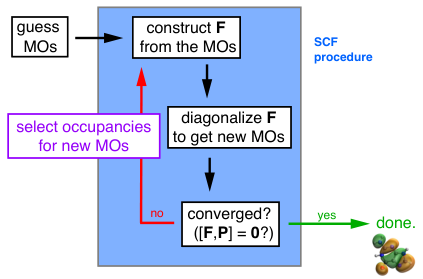
A flowchart of the SCF procedure is illustrated in Fig. 11. At each iteration, the occupied MOs are used to construct the Fock matrix , which is then diagonalized to obtain new MOs. Notably, diagonalization results in MOs and one must decide how to choose the occupied set. Ordinarily, the lowest eigenvalues are selected (aufbau principle), resulting in the ground-state determinant upon SCF convergence. To locate an excited-state SCF solution instead, one seeds the procedure with initial-guess MOs from a ground-state calculation but with non-aufbau occupancies, promoting an electron from HOMO to LUMO, for example. This makes the LUMO into an occupied level and the HOMO into a virtual level, resulting in a “hole”, i.e., a virtual level whose energy lies below that of the highest occupied level. When the Fock matrix is constructed from this new set of occupied MOs and then diagonalized, the question becomes which of the new MOs should be the occupied ones, since energy levels may have shifted. The SCF procedure therefore deviates from the usual one only when it comes to selecting the occupied subset from among the MOs. Several different options have been explored, as discussed in the next section.
Before reviewing algorithms for locating non-aufbau SCF solutions, however, it is important to note some properties of those solutions that are different from ground-state properties. First, because the effective Hamiltonian depends on the MOs themselves, the ground- and excited-state Slater determinants are eigenfunctions of different Hamiltonians and are therefore not orthogonal. One consequence is that the formula for oscillator strengths in terms of transition dipole matrix elements [Eq. (3)] is not strictly valid,349 as that formula is derived using the assumption that the eigenfunctions of the Hamiltonian form a complete orthonormal set.44 In small-molecule tests, however, overlap integrals between ground- and excited-state determinants are found to be .342
Another general concern is that excited states are always open-shell species, even if the ground state is closed-shell, so any single-determinant approximation is certain to be spin-contaminated, perhaps badly so. Indeed, single-determinant approximations for open-shell singlet states are often characterized by (in atomic units of ), which is equal to the average of pure-state singlet and triplet values. A similar phenomenon occurs, for similar reasons, in the case of the spin-unrestricted Hartree-Fock wave function in the separated-atom limit,59 because a spin-pure state with two half-filled orbitals can be described using a minimum of two Slater determinants. The same two determinants (with different relative signs) are needed to describe both singlet spin-coupling (total ) as well as the component of triplet spin-coupling ().
In practice, SCF excitation energies for open-shell singlet excited states are often surprisingly accurate despite significant spin contamination,342, 344, 350 although there are exceptions. One such exception is the 1B1u state of ethylene, whose underestimation by almost 2 eV is attributed to severe spin contamination.342 Yamaguchi and co-workers have developed spin-projection techniques that can be used to recover spin-pure states in such cases,351, 352, 353, 354 and approximate spin purification is often used as a practical workaround in “broken-symmetry” DFT calculations of transition metal complexes.355, 354, 353 For an open-shell singlet, the most common approach is to approximate the singlet energy as
| (66) |
Here, is the energy of the contaminated (mixed-spin or broken-symmetry) state that is obtained in searching for a singlet solution, whereas is the triplet energy for the same system, for which spin contamination is typically less severe. This procedure has a long history,356, 355 and Eq. (66) can be viewed as an approximate form of spin projection, generalizable to cases where the target state has spin .352 The formula in Eq. (66) is sometimes implemented in a self-consistent way, i.e., using Eq. (66) as the ansatz and minimizing with respect to orbital rotations. That method is known as restricted open-shell Kohn-Sham (ROKS) theory,357, 358, 359 and it affords a common set of orbitals for both multiplicites. More often, however, Eq. (66) is used as an a posteriori correction scheme.360, 340, 361, 362, 363, 364, 365, 366 Even then, Eq. (66) can easily be used in geometry optimizations (at the cost of two energy and gradient evaluations per step) and in vibrational frequency calculations.340 For the aforementioned 1B1u state of C2H4, application of Eq. (66) reduces the SCF error (as compared to experiment) from 1.8 eV to 0.3 eV.342
3.1.2 Orbital-Optimized Non-Aufbau SCF Solutions
The simplest means to construct a non-aufbau occupied set is known as the maximum overlap method (MOM).342, 343, 344, 345 Starting from an initial guess corresponding to non-aufbau occupation of the ground-state MOs, this approach uses an overlap criterion to identify the new MOs at each subsequent SCF iteration. To do this, one must compute the projections of the MOs at the th iteration onto a reference set of MOs. The reference set might be the MOs at the previous iteration, in which case
| (67) |
or else it could be the initial set of ground-state MOs, :
| (68) |
The first choice [Eq. (67)] represents the original version of the algorithm,342 whereas Eq. (68) has been called the “initial MOM” (IMOM) algorithm and tends to have better success at converging orbital-relaxed non-aufbau states.344 The signature of success is a “hole below the Fermi level”, i.e., a virtual MO whose energy is lower than the HOMO energy.
The MOM and IMOM algorithms consist simply in replacing the aufbau selection of occupied MOs with a selection based on the largest values of the overlaps . All other aspects of the SCF algorithm remain the same. This approach exhibits the same cost per SCF iteration as the ground-state algorithm and when it succeeds, the rate of convergence (measured in number of SCF cycles) is typically on par with a conventional ground-state calculation. There are certainly cases where MOM and IMOM fail,347, 348 however, typically resulting in variational collapse to the ground-state SCF solution. In such cases, more robust SCF convergence algorithms are required.
One such approach is the “-SCF” method,346 which is based on minimizing the functional
| (69) |
for a specified energy . This idea stems from recognizing that eigenstates satisfy the zero-variance condition . The -SCF approach avoids variational collapse by solving a proper minimization problem, but the appearance of means that four-particle operators are required and the requisite transformations endow this method with scaling.346 This makes the -SCF approach much more expensive than conventional SCF theory.
An alternative approach with the same formal scaling as the ground-state SCF problem is squared-gradient minimization (SGM).347 Here, the idea is to convert an inherently unstable saddle-point optimization into a search for a local minimum by optimizing an objective function equal to the squared gradient of the energy with respect to orbital rotations. A local minimum can always be converged (if slowly), whereas a saddle point can be missed, and this makes SGM more robust as compared to MOM or IMOM. While the cost remains , it is 2–3 times more expensive per SCF iteration as compared to a conventional SCF calculation, due to the cost of constructing the objective function.347 It is also known that the squared gradient of a function may contain minima that do not correspond to stationary points of the original function.367, 368, 369, 370 From the standpoint of trying to locate an orbital-relaxed excited-state Slater determinant, these are spurious solutions.
A middle way between MOM and SGM is state-targeted energy projection (STEP),348 which does not increase the cost per SCF iteration yet shows much more robust convergence behavior as compared to MOM or IMOM. The STEP approach constructs a projection operator onto the virtual space,
| (70) |
where the summation runs over some or all of the virtual MOs. The matrix representation of is , where consists of column vectors corresponding to whichever MOs are included in Eq. (70). The Fock matrix is then modified according to
| (71) |
where is the atomic orbital (AO) overlap matrix. The effect of the additional term is to shift all of the orbitals that are included in Eq. (70) by an energy . By pre-selecting a virtual MO from the ground-state calculation that will be occupied in the first iteration of STEP, one can modify the Fock matrix to shift other virtual orbitals (including a lower-energy one that was occupied in the ground state but whose electron was promoted) to energies above the non-aufbau orbital. For example, upon promotion, the original HOMO is unoccupied and should be included in Eq. (70), whereas the LUMO becomes occupied and should be excluded from . The STEP algorithm is a form of level-shifting that tends to ensure that the SCF algorithm converges to the “closest” stationary point in the space of MO coefficients, which therefore resembles the initial guess.348 Like MOM and IMOM, STEP can be used in conjunction with ground-state gradient technology to perform geometry optimizations and vibrational frequency calculations.
3.1.3 Transition Potential Methods
The methods described in Section 3.1.2 involve state-specific orbital optimization, meaning that the SCF procedure must be iterated to convergence separately for each excited state of interest. This has the advantage of including full orbital relaxation effects (beyond LR theory), but the disadvantage that there is no guarantee that an excited state resembling the one of interest can actually be found. A simpler (if cruder) approach was devised long ago by Slater,371, 372 and forms the basis of several popular techniques for estimating x-ray excitation energies from Kohn-Sham eigenvalues.373, 374, 375, 376, 377
To understand Slater’s method, imagine that is the energy of a single-determinant wave function with orbital occupation numbers , some of which might be fractional. Expanding the energy as a Taylor series around a reference energy , keeping the orbitals fixed, one obtains
| (72) |
According to the Slater-Janak theorem,378 the first derivative is an orbital eigenvalue: . Now consider promotion of one electron from an occupied MO to a virtual MO. It suffices to deal with just a pair of occupancies , in terms of which the transition in question can be abbreviated as . If a fractional-occupancy state with is used for the reference , then using Eq. (72) to compute the excitation energy leads to an estimate
| (73) |
where the approximation neglects terms of order .374 This forms the basis of the Slater transition method (STM), wherein an SCF calculation is carried out for the fractional-occupancy state and then the energy difference affords an estimate of the excitation energy.
Variants of STM have historically been popular for x-ray spectroscopy,373, 374, 375, 376, 377 particularly in the context of periodic DFT calculations where LR-TDDFT with semilocal functionals is problematic.21 In principle this method requires a separate SCF calculation for each excitation of interest, and while it is generally easy to converge the x-ray “edge” in this way (i.e., a core LUMO transition), higher-lying states will require a convergence algorithm that can avoid variational collapse. Moreover, this state-by-state approach leads to nonorthogonal MOs and therefore exhibits the same ambiguities regarding oscillator strengths as the SCF method.349 For these reasons, it is common to omit the electron in the virtual space (with only pragmatic justification), leaving in the core-excited MO. This variant of the procedure has been called the transition potential (TP) method.379, 380, 381, 382, 377 By neglecting to occupy any core-excited virtual states at all, this approach sidesteps the issue of nonorthogonality, at least for a given choice of . Oscillator strengths can be computed in a straightforward way from matrix elements constructed from the orbitals obtained from the fractional-occupancy SCF calculation.
Modifications to the formula in Eq. (73) have also been proposed,383, 384, 377, 385 sometimes involving more than one SCF calculation with differing fractional occupancies, or by combining eigenvalues of both the neutral molecule and its cation or anion.386, 387 These modifications represent attempts to eliminate higher-order errors in Eq. (72). An example is the “generalized STM” (gSTM) method,383, 377 which replaces Eq. (73) with
| (74) |
This is based on an alternative approximation for the integral
| (75) |
The original STM in Eq. (73) corresponds to a midpoint approximation for this integral.383, 377 The gSTM approach requires two separate SCF calculations, one with and the other with .
Variants that set (removing the entirety of the core electron) have also been suggested and are sometimes called “full core hole” (FCH) methods.373, 374, 375, 376, 377 The TP approach is then a “half core hole” (HCH) method. Although the FCH approach deviates significantly from Slater’s original idea, it can be conceptualized as an attempt to restore charge balance, once the 1/2 electron in the virtual space has been abandoned for reasons of convenience. The excited core hole (XCH) approach388 is yet another variant that creates a charge-neutral state (which is important for periodic DFT calculations) by placing the excited electron in the LUMO and using the full virtual spectrum from that calculation:388, 377
| (76) |
Together, these STM- and TP-type procedures are known as occupancy-constrained SCF methods. In that context there has been some discussion of “many-electron” effects on oscillator strengths for x-ray transitions.389, 390 What “many-electron” means in this context is multi-determinant character in the final state, which is of course included automatically in a LR-TDDFT calculation.
3.2 Examples
The primary purpose of this chapter is to survey methods rather than applications but we will highlight a few recent applications of the SCF approach in order demonstrate that it can be an elegant and low-cost alternative in cases where LR-TDDFT performs poorly, such as CT states.391, 338 Whereas LR-TDDFT systematically (and sometimes dramatically) underestimates CT excitation energies, the same excitation energies are systematically overestimated by the uncorrelated CIS method.392 At the CIS level, a long-range excitation uses up the one occupied virtual excitation that is included in the ansatz and leaves no excitations to facilitate orbital relaxation around either the electron or the hole, hence the overestimation. LR-TDDFT and CIS may therefore bracket the correct answer for a CT state but these upper and lower bounds can be several electron volts apart!255 The SCF approach includes full orbital relaxation and is also less sensitive to the asymptotic behavior of the XC potential. There has also been some preliminary work on the description of conical intersections and nonadiabatic dynamics using SCF methods.339, 393

States with double-excitation character represent another categorical failure of LR-TDDFT within the adiabatic approximation,99 with the most famous example being the optically-dark S1(21A) state in carotenoids,395, 396, 397 or the analogous 21A state in butadiene and other conjugated polyenes.398, 399, 400, 401, 402 Doubly-excited states can be captured accurately using SCF methods,347, 348, 338 as shown for a few examples in Fig. 12. For these challenging cases, taken from a benchmark data set of double excitations,394 several mGGA and hybrid functionals prove to be significantly more accurate than the CC3 method, which includes triple excitations and is generally close to CCSD(T) in quality,403 with similar scaling.404 For the full data set from Ref. 394, the hybrid GGA functional B97X-V achieves a mean absolute error (MAE) of 0.6 eV and a maximum error of 1.1 eV, whereas for CC3 the MAE is 1.0 eV and the maximum error is 1.8 eV.348 The mGGA functional B97M-V does even better, with a MAE of 0.15 eV and a maximum error of 0.46 eV.348

The SCF methodology can also be used to compute an electronic absorption spectrum, although this must be done one state at a time by converging a sequence of non-aufbau determinants representing each excited state, and there is no guarantee that some states are not accidentally omitted. A successful example is shown in Fig. 13, reproducing the absorption spectrum of the chlorophyll molecule that was only recently measured in the gas phase.406, 405 Using a STEP-based SCF procedure, the major peaks in that spectrum can be identified with transitions amongst the frontier MOs,348 confirming the basic picture of Gouterman’s four-orbital model.407 LR-TDDFT calculations of the same molecule require twice as many states in order to resolve the spectrum up to 300 nm. Many of these states have near-zero oscillator strengths,405 suggesting possible contamination by spurious CT states.
| Functional | K edgeb | L2,3 edgesc | |||
|---|---|---|---|---|---|
| mean | RMSE | mean | RMSE | ||
| LDA | 4.4 | ||||
| PBE | 0.9 | ||||
| B97M-V | 1.8 | ||||
| SCAN | 0.2 | 0.2 | |||
| PBE0 | 0.6 | ||||
| B97X-V | 0.4 | 0.4 | |||
- •
aData from Ref. 408, using the SGM algorithm and aug-cc-pCVTZ basis set. bData set includes 40 transitions for C, N, O, and F atoms. Error is defined with respect to experiment, with atom-specific scalar relativistic effects included in the calculation. cIncluding spin-orbit effects.
Core–valence excitation energies are fertile ground for SCF techniques. These states appear at photon energies eV and therefore it is not feasible to reach them by iterative solution of an eigenvalue problem starting from the lowest excitation energies. The frozen-valence approximation is one way to reach these states in LR-TDDFT, which is very accurate for K-edge transitions177 but may be questionable for L- or M-edge excitations. Fortunately, core-to-LUMO excitations are relatively easy to locate using MOM.343 Table 1 shows some error statistics for a benchmark set of K- and L-edge transitions.408 Except for the LDA functional, all of the errors are eV and several functionals achieve errors eV, in excitation energies that are hundreds of electron volts. Notably, some of these same functionals also afford accurate L-edge transition energies, if spin-orbit interactions are included in order to describe the splitting of the 2p subshell into 2p1/2 and 2p3/2 states.164 This splitting can be quite large, e.g., eV for Fe(II).409, 410 Errors of eV are also possible for heavier elements using ROKS with relativistic corrections.411
This excellent performance is perhaps somewhat surprising due to the substantially different self-interaction errors in core versus valence orbitals.412, 413 The “optimal tuning” of LRC functionals that was described in Section 2.3.1, in which the range-separation parameter is adjusted to set , can be understood as an attempt to cancel the self-interaction error associated with the HOMO, but that is likely to leave residual self-interaction in the much more compact core orbitals. These errors are exposed in SCF calculations of core-level electron binding energies (for x-ray photoelectron spectroscopy), where many functionals afford errors eV for transition metals.414 Even the SCAN functional, which performs well for core-excited states of second-row atoms (Table 1), affords errors of eV for core-level binding energies.415 In several cases, Hartree-Fock theory proves to be more accurate than standard functionals that include correlation, even upon accounting for relativistic corrections.416, 414 This is consistent with other results indicating that the restricted open-shell (RO-)CIS method is a reasonable level of theory for M- and L-edge spectra of solid-state transition metal oxides, despite its lack of correlation effects, provided that spin-orbit corrections are included.417 Resolution of this apparent paradox remains an open question.
| Method | Functional | Molecule | Errorc | |||
|---|---|---|---|---|---|---|
| HF | CH4 | HF | CH4 | |||
| LR-TDDFT | SCAN | 666.1 | 273.8 | |||
| SCF +ASPb | SCAN | 687.1 | 287.9 | |||
| ROKS | SCAN | 687.0 | 288.0 | |||
| LR-TDDFT | B97X-V | 668.7 | 276.5 | |||
| SCF +ASPb | B97X-V | 687.2 | 288.5 | |||
| ROKS | B97X-V | 687.1 | 288.5 | |||
| Experiment | 687.4 | 288.0 | — | — | ||
For second-row atoms, errors in both core-level IEs343, 416, 418 and also core-level excitation energies343, 408, 348 are comparatively small when using the SCF approach, although even for these elements Hartree-Fock theory is competitive with DFT,418 suggesting that orbital relaxation is much more important than correlation. These rather small errors should be contrasted with much larger ones encountered when LR-TDDFT is applied to the same states using the frozen-valence approximation. Table 2 shows results for two different molecules (HF and CH4) using two different functionals (SCAN and B97X-V) that both perform well in SCF benchmarks. In contrast to the sub-eV errors obtained using the SCF approach, LR-TDDFT calculations exhibit errors in excess of 10 eV for the carbon K-edge transition and eV for the fluorine K-edge transition. For K-edge transitions of Mn(II) at eV, LR-TDDFT errors of eV are obtained using B3LYP, and errors using the GGA functional BP86 are eV.419 Errors are even larger for heavier elements.420 Notably, the sign of the errors in Table 2 points to underestimation of the excitation energy, consistent with too-soft asymptotic decay of the potential for a transition with CT character from a very compact 1s orbital to a radially-diffuse LUMO. LRC functionals perform much better in this capacity.421, 422
That said, the precision of core excitation energies computed using LR-TDDFT is rather good even if the accuracy is not,422 meaning that chemical shifts can be obtained even if absolute excitation energies must be shifted to match experiment. It is the magnitude of the required shifts that is somewhat unnerving. This inspired work on RSH functionals that partition into short-, middle-, and long-range components,211, 212, 213, 214 with the intention to use a larger fraction of exact exchange () at a length scale Å.423 These “short-range corrected” (SRC) functionals work rather well for LR-TDDFT x-ray calculations,213 although they are empirically parameterized specifically for that purpose and may not be good functionals for other applications such as ground-state thermochemistry or valence excitation energies. Furthermore, the SRC functionals are not LRC functionals in the sense of Eq. (48), because they do not go to a limit of 100% HFX as . Proper LRC functionals have been developed to describe core-level excitations.211

As illustrated by the porphyrin spectrum in Fig. 13 and other examples,338 accurate electronic absorption spectra can be computed via SCF calculations that are carried out in a state-by-state manner. However, this does present something of a nuisance as compared to automatic generation of numerous excitation energies in a LR-TDDFT calculation. Some of the TP or occupancy-constrained SCF approaches that were described in Section 3.1.3 bypass this annoyance by using orbital eigenvalues from one or two fractional-occupancy SCF calculations to obtain the entire spectrum of excitation energies. These methods are assessed (versus experiment) in Fig. 14, for a data set of K-edge transitions.377 Following the notation of Ref. 377, these methods are characterized as either “explicit” or “implicit”, with explicit methods involving occupancy constraints that are applied state-by-state, as suggested by the original Slater method, whereas the implicit methods place no electron at all into the virtual space, which makes for a very simple computational scheme. The “neutral implicit” methods follow the paradigm of the XCH approach,388 placing an electron (or a fraction of an electron) into the LUMO only; it is often possible to optimize a core-to-LUMO SCF solution without specialized algorithms. Finally, the “ground state” results in Fig. 14 represent a control experiment in which the ground-state eigenvalue difference is used to approximate the K-edge transition energy. That method fares surprisingly well, or perhaps the other approaches should be said to fare surprisingly poorly. If the user desires to avoid state-by-state optimization of an occupancy-constrained determinant, then the XCH approach would seem to be the best option.
4 Time-Dependent Kohn-Sham Theory: “Real-Time” TDDFT
The cost of the SCF approaches described in Section 3 is typically no more than a few times the cost of ground-state DFT, depending somewhat on the algorithm that is used to converge the non-aufbau SCF solution. With the exception of the -SCF method, the algorithms described in that section each possess the same scaling as the ground-state calculation. However, these methods must be applied in a state-by-state manner, constructing a different initial guess for each state of interest, which limits their applicability to problems where only a small number of states is desired or required. In contrast, using LR-TDDFT it is possible to obtain a large number of states in an automated fashion, at least for medium-sized molecules. For large molecules, the cost of computing a very large number of excited states can become prohibitively expensive, especially in systems where the density of states is large. The appearance of spurious CT states in the spectrum exacerbates the cost, even if their affect on the overall spectral envelope is nil.286, 424 In situations such as these, where proliferation of states (whether real or spurious) makes the iterative diagonalization cost-prohibitive, the TDKS approach may be advantageous. Using this method, a broadband spectrum can be computed from the oscillating dipole moment function obtained from time-dependent electron dynamics.
4.1 Theory
The TDKS approach is also known as “real-time” (RT-)TDDFT,51, 52 to distinguish it from LR-TDDFT. Starting from the ground-state Kohn-Sham determinant, an external electric field is turned on at , either as an impulse or as a continuous wave, and the resulting perturbation creates a time-evolving superposition state whose Fourier components encode the excitation energies. This is analogous to propagation of a non-stationary wave packet according to the time-dependent Schrödinger equation. Similar to that situation, the time-dependent MOs are complex-valued for . Unlike the many-electron time-dependent Schrödinger equation, the effective Hamiltonian in Kohn-Sham theory depends on its own time-evolving eigenfunctions, and does not commute with for . Therefore the time evolution operator
| (77) |
for time-independent Hamiltonian must be generalized to
| (78) |
for TDKS calculations, where is a time-ordering operator. This leads to so-called Magnus expansion that generalizes the time-independent Baker-Campbell-Hausdorff expansion.425, 426, 427
A variety of time-propagation algorithms have been developed for TDKS simulations,428, 429, 430, 431, 427, 52 the simplest of which is a “modified-midpoint” algorithm,429 a type of explicit Euler integration scheme that requires only one Fock matrix construction per time step. Denoting the Fock and density matrices in the orthonormal MO basis as and , respectively, the Fock matrix is first propagated forward in time by a half step, . At each subsequent instant in time, , the matrix representation of the propagator is constructed according to
| (79) |
again in the MO basis.427 The MO density matrix is then propagated from to according to
| (80) |
(Spin indices are omitted as these equations are valid for either spin.) Construction of requires diagonalization of the Fock matrix, which is not a problem in Gaussian basis sets but is not feasible in plane-wave basis sets or on a grid. See Ref. 428 for a discussion of alternatives when is too large to diagonalize. For Gaussian basis calculations, self-consistent propagators based on predictor–corrector algorithms have also been developed.427, 432 These may require more than one Fock build per time step but allow for the use of somewhat larger time steps as well as for automatic detection of time steps that are too long, which is not always obvious from the usual criterion of checking to make sure that fluctuations in the total energy are bounded.427
For the modified-midpoint algorithm that is encapsulated by Eqs. (79) and (80), the cost of a single time step is comparable to the cost of a single SCF cycle of the ground-state calculation. The storage requirement is also modest, amounting to a few complex-valued matrices of dimension . This should be contrasted with the storage requirement for iterative solution of the LR-TDDFT pseudo-eigenvalue problem, which is with a prefactor that reflects the number of iterations and therefore the size of the iterative subspace. The modified-midpoint approach works well provided that the time step is sufficiently small; values ranging from 0.01–0.50 a.u. are typical, where s = 24.2 attoseconds. (The time for one orbit in the Bohr model of the hydrogen atom is times this value, which establishes a timescale for electronic motion.) The maximum acceptable value of is limited not only by stability of the time integration but also by the excitation energies that one desires to access, as discussed below.
Unlike LR-TDDFT, which operates by definition in the limit of a vanishingly weak external field, the TDKS approach is non-perturbative and in principle can be used to simulate electron dynamics in strong laser fields, e.g., to simulate nonlinear optical properties of materials,433 or to make contact with emerging attosecond spectroscopies57 that create electronic wave packets that are out of equilibrium with the nuclei and thus outside of the Born-Oppenheimer approximation.54, 53, 55, 56 In practice, there are various issues related to the use of the adiabatic approximation (Section 2.1.2),434, 435, 290 meaning the use of ground-state functionals with no memory, such that the time dependence is carried solely by the time-evolving density, . On the other hand, within the adiabatic approximation the initial-state dependence vanishes since the XC kernel is fully specified in terms of the instantaneous time-evolving density.436 The topic of strong-field electron dynamics and how it can be described using TDKS calculations is not considered here, except to note that there have been successful TDKS simulations of strong-field photoionization,437, 438, 439, 440, 441, 442, 443, 444, 445, 446, 447, 448 and also of high harmonic generation,449, 450, 451, 452, 453, 454, 455, 456, 457 both in Gaussian-orbital representations of the density. Unlike the grid-based treatments that are common in atomic physics, Gaussian-based methods are scalable to molecules. However, self-interaction error is known to significantly suppress strong-field ionization rates,458 therefore much of the aforementioned work has been performed at the TD-CIS level, where self-interaction is not a concern and the exchange potential has the correct asymptotic form.
This section focuses on the use of TDKS simulations to obtain broadband spectra. Within the electric dipole approximation (which is also invoked in LR-TDDFT insofar as oscillator strengths are proportional to transition dipole matrix elements), the absorption spectrum corresponds to the dipole strength function459, 163
| (81) |
where for example
| (82) |
is an element of the dynamic polarizability tensor, . The quantities and are the Fourier transforms of the time-dependent dipole moment and the external electric field, respectively, although for an impulsive -function pulse the denominator in Eq. (82) can be replaced by the field amplitude while the numerator is replaced by
| (83) |
Here, is a windowing or padding function, as in standard signal processing.52 To obtain a linear absorption spectrum the external field should be weak, impulsive, and off-resonant, and should contain components in all three Cartesian directions in order to excite states of all symmetries, effectively averaging over molecular orientations. With an appropriately chosen integration time step, this procedure reproduces the same spectrum that is obtained using LR-TDDFT, if all of the LR-TDDFT excitations within the energy window of interest are included.459, 427 The TDKS approach affords the entire broadband spectrum from a single Fourier transform [Eq. (83)] following sufficient time propagation, but it is not straightforward to assign the features in the TDKS spectrum to transitions between specific MOs. Techniques to do so have been developed, based on identifying individual Fourier modes in the dipole moment matrix (expressed in the MO basis) at a specific transition frequency.460, 461, 462, 463, 464 This does require some post-processing and some insight regarding the important MOs. Time-dependent generalization of the NTO basis (Section 2.2.4) have also been proposed.465
The cost of the time steps needed to propagate the Kohn-Sham MOs in time, and thus to obtain the time-evolving density and dipole moment function, is comparable to the cost of a single ground-state SCF cycle but many time steps are required. A typical simulation time might be 30 fs to obtain a fully-converged spectrum,427 but with as (1 as = s), this represents time steps. Recently, Padé approximant techniques have been introduced in order to obtain based on a short time series of input data .462, 52 Using this approach, spectra that are well-converged (with respect to LR-TDDFT results) can be obtained in fs of time propagation and rough spectra can be obtained with as little as 3–5 fs.163 The time step dictates the spectral window that can be accessed, via the usual time-energy uncertainty relationship that comes from the Fourier transform. In practice, the spectrum is only reliably converged up the Nyquist frequency , and perhaps only a fraction of that value.427, 163 This implies that especially small time steps are required for x-ray applications. A time step a.u., for example, corresponds to a Nyquist frequency eV, which is well above the K edge for second-row elements (C, N, O, etc.) but not for third-row elements. The K edge for elements Al–Cl lies above 1,500 eV.
4.2 Examples

As an example of a broadband spectrum of interest in materials science, Fig. 15 presents x-ray spectra at the L2,3 edge of -quartz, computed using several different TDDFT methods.467 Starting from the lowest valence excitations, a LR-TDDFT calculation with reproduces the first two features in the experimental spectrum (labeled “A” and “B”) but is unable to resolve the higher-energy features. (The calculations do not include spin-orbit coupling and thus do not reproduce the doublet for peak A, which arises due to the 0.6 eV splitting of the 2p3/2 and 2p1/2 levels.466) Although the most intense feature (peak B) is evident in the RT-TDDFT spectrum, at a peak position that precisely matches the corresponding LR-TDDFT spectrum, the RT-TDDFT spectrum is quite noisy and other features in that spectrum are obscured by this noise.
That noise is actually a basis-set artifact arising from the absence of proper continuum states (or the inability to describe ionization within a finite-basis approximation), which has the effect of artificially trapping metastable excitations that lie above the ionization threshold.468, 467 A solution to this problem is to incorporate phenomenological lifetimes for the unbound MOs, meaning those with . This procedure is described in Ref. 468 and corresponds to a modification in the MO basis, where is a phenomenological lifetime that is modeled as a function of energy, decreasing exponentially above the vacuum level. As seen in Fig. 15, this “” modification removes the noise from the RT-TDDFT spectrum, such that most of the experimental features become evident even at energies far above what can feasibly be reached with LR-TDDFT. This does require some phenomenological modeling, however.

When computing K-edge x-ray spectra using high-quality basis sets, similar artifacts can manifest as spurious pre-edge features that are not seen in compact basis sets where the density of levels is more sparse. In a molecule that contains both nitrogen and oxygen, for example, excitations from N(1s) core orbitals to the highest-energy virtual MOs can manifest as spurious pre-edge features at the oxygen K-edge,163, 469 as shown in Fig. 16. These artifacts appear despite the fact that the nitrogen K-edge lies eV below the oxygen K-edge! These intruder peaks could potentially be mitigated via heuristic lifetime models for the unbound states, as described above, although a simpler fix is to modify the time-dependent dipole moment matrix in the MO basis. That matrix is
| (84) |
for the component. The time-dependent dipole moment function that is needed in Eq. (83) is then
| (85) |
By eliminating the rows and columns of that correspond to occupied MOs other than the ones of interest, prior to computing the Fourier transform in Eq. (83), the undesired resonances can be removed from the spectrum.469 For the oxygen K edge, this means retaining only those rows and columns where and refer to the O(1s) orbitals. This is precisely analogous to the frozen-valence truncation of the LR-TDDFT excitation manifold that is used to obtain core-level spectra (Section 2.2.1), and may have similar limitations for L- and M-edge spectra. For the oxygen K edge, Fig. 16 shows that this procedure affords a spectrum in good agreement with LR-TDDFT, free of contamination by N(1s) excitations. This filtering procedure does require the user to decide in advance which edges are of interest, so that multiple edges can no longer be computed in a single calculation unless the entire trajectory of dipole moment matrices is stored.
The TDKS approach has been extended to compute excited-state absorption spectra,436, 470 using an excited-state density prepared via LR-TDDFT as the initial density at . Because the initial state is non-stationary, this requires that the “field on” simulation be referenced to a time-evolving “field-off” simulation.436 This approach has recently been applied to simulate emerging transient x-ray experiments,471, 472, 473, 474 carried out at free-electron laser facilities using x-ray pulses with femtosecond time resolution. As an example, it is possible to follow metal-to-metal CT dynamics in the mixed-valence compound, which occur on a fs timescale following excitation at 800 nm, using time-resolved x-ray emission spectroscopy at the iron K edge ( transition at 7,114 eV).474
Acknowledgements
The author’s work on excited-state DFT has been supported for many years by the U.S. National Science Foundation, at present under grant no. CHE-1955282.
References
- 1 J. A. Pople, P. M. W. Gill, and B. G. Johnson, “Kohn–Sham density-functional theory within a finite basis set”, Chem. Phys. Lett., 199, 557–560 (1992).
- 2 P. M. W. Gill, B. G. Johnson, J. A. Pople, and M. J. Frisch, “The performance of the Becke–Lee–Yang–Parr (B–LYP) density function theory with various basis sets”, Chem. Phys. Lett., 197, 499–505 (1992).
- 3 B. G. Johnson, P. M. W. Gill, and J. A. Pople, “Preliminary results on the performance of a family of density functional methods”, J. Chem. Phys., 97, 7846–7848 (1992).
- 4 B. G. Johnson, P. M. W. Gill, and J. A. Pople, “The performance of a family of density functional methods”, J. Chem. Phys., 98, 5612–5626 (1993).
- 5 C. W. Murray, G. J. Laming, N. C. Handy, and R. D. Amos, “Kohn–Sham bond lengths and frequencies calculated with accurate quadrature and large basis sets”, Chem. Phys. Lett., 199, 551–556 (1992).
- 6 G. J. Laming, N. C. Handy, and R. D. Amos, “Kohn-Sham calculations on open-shell diatomic molecules”, Mol. Phys., 80, 1121–1134 (1993).
- 7 H. Weiss, R. Ahlrichs, and M. Häser, “A direct algorithm for self-consistent-field linear response theory and application to C60: Excitation energies, oscillator strengths, and frequency-dependent polarizabilities”, J. Chem. Phys., 99, 1262–1270 (1993).
- 8 R. Bauernschmitt and R. Ahlrichs, “Treatment of electronic excitations within the adiabatic approximation of time dependent density functional theory”, Chem. Phys. Lett., 256, 454–464 (1996).
- 9 M. Petersilka, U. J. Gossmann, and E. K. U. Gross, “Excitation energies from time-dependent density-functional theory”, Phys. Rev. Lett., 76, 1212–1215 (1996).
- 10 R. E. Stratmann, G. E. Scuseria, and M. J. Frisch, “An efficient implementation of time-dependent density-functional theory for the calculation of excitation energies of large molecules”, J. Chem. Phys., 109, 8218–8224 (1998).
- 11 S. Hirata and M. Head-Gordon, “Time-dependent density functional theory within the Tamm-Dancoff approximation”, Chem. Phys. Lett., 314, 291–299 (1999).
- 12 T. Grabo, M. Petersilka, and E. K. U. Gross, “Molecular excitation energies from time-dependent density functional theory”, J. Mol. Struct. (Theochem), 501–502, 353–367 (2000).
- 13 M. E. Casida, “Time-dependent density functional response theory for molecules”, in Recent Advances in Density Functional Methods, Part I, D. P. Chong, Ed., Vol. I of Recent Advances in Computational Chemistry; World Scientific: River Edge, NJ, 1995; chapter 5, pages 155–192.
- 14 M. E. Casida, “Time-dependent density functional response theory of molecular systems: Theory, computational methods, and functionals”, in Recent Developments and Applications of Modern Density Functional Theory, J. M. Seminario, Ed., Vol. 4 of Theoretical and Computational Chemistry; Elsevier: Amsterdam, 1996; pages 391–439.
- 15 F. Furche, “On the density matrix based approach to time-dependent density functional response theory”, J. Chem. Phys., 114, 5982–5992 (2001).
- 16 A. McLachlan and M. Ball, “Time-dependent Hartree-Fock theory for molecules”, Rev. Mod. Phys., 36, 844–855 (1964).
- 17 N. T. Maitra, “Perspective: Fundamental aspects of time-dependent density functional theory”, J. Chem. Phys., 144, 220901:1–16 (2016).
- 18 A. D. Laurent and D. Jacquemin, “TD-DFT benchmarks: A review”, Int. J. Quantum Chem., 113, 2019–2039 (2013).
- 19 F. Furche and D. Rappoport, “Density functional methods for excited states: Equilibrium structure and electronic spectra”, in Computational Photochemistry, M. Olivucci, Ed., Vol. 16 of Theoretical and Computational Chemistry; Elsevier: Amsterdam, 2005; chapter 3, pages 93–128.
- 20 S. Hirata, M. Head-Gordon, and R. J. Bartlett, “Configuration interaction singles, time-dependent Hartree–Fock, and time-dependent density functional theory for the electronic excited states of extended systems”, J. Chem. Phys., 111, 10774–10786 (1999).
- 21 M. E. Casida, “Time-dependent density-functional theory for molecules and molecular solids”, J. Mol. Struct. (Theochem), 914, 3–18 (2009).
- 22 C. A. Ullrich and Z.-H. Yang, “Excitons in time-dependent density-functional theory”, in Density-Functional Methods for Excited States, N. Ferré and M. Filatov, Eds., Vol. 368 of Topics in Current Chemistry; Springer International Publishing: Switzerland, 2016; pages 185–218.
- 23 E. Tapavicza, G. D. Bellchambers, J. C. Vincent, and F. Furche, “Ab initio non-adiabatic molecular dynamics”, Phys. Chem. Chem. Phys., 15, 18336–18348 (2013).
- 24 M. Barbatti and R. Crespo-Otero, “Surface hopping dynamics with DFT excited states”, in Density-Functional Methods for Excited States, N. Ferré, M. Filatov, and M. Huix-Rotllant, Eds., Vol. 368 of Topics in Current Chemistry; Springer International Publishing: Switzerland, 2016; pages 415–444.
- 25 S. M. Parker, S. Roy, and F. Furche, “Multistate hybrid time-dependent density functional theory with surface hopping accurately captures ultrafast thymine photodeactivation”, Phys. Chem. Chem. Phys., 21, 18999–19010 (2019).
- 26 X. Zhang and J. M. Herbert, “Nonadiabatic dynamics with spin-flip versus linear-response time-dependent density functional theory: A case study for the protonated Schiff base C5H6NH”, J. Chem. Phys., 155, 124111:1–15 (2021).
- 27 J. M. Herbert and A. Mandal, “Spin-flip TDDFT for photochemistry”, in Time-Dependent Density-Functional Theory: Nonadiabatic Molecular Dynamics, C. Zhu, Ed. (To be published by Jenny Stanford. Preprint available at DOI: 10.26434/chemrxiv-2022-gj75d).
- 28 M. Huix-Rotllant, A. Nikiforov, W. Thiel, and M. Filatov, “Description of conical intersections with density functional methods”, in Density-Functional Methods for Excited States, N. Ferré, M. Filatov, and M. Huix-Rotllant, Eds., Vol. 368 of Topics in Current Chemistry; Springer International Publishing, 2016; pages 445–476.
- 29 S. Gozem, M. Huntress, I. Schapiro, R. Lindh, A. A. Granovsky, C. Angeli, and M. Olivucci, “Dynamic electron correlation effects on the ground state potential energy surface of a retinal chromophore model”, J. Chem. Theory Comput., 8, 4069–4080 (2012).
- 30 S. Gozem, F. Melaccio, R. Lindh, A. I. Krylov, A. A. Granovsky, C. Angeli, and M. Olivucci, “Mapping the excited state potential energy surface of a retinal chromophore with multireference and equation-of-motion coupled-cluster methods”, J. Chem. Theory Comput., 9, 4495–4506 (2013).
- 31 S. Gozem, F. Melaccio, A. Valentini, M. Filatov, M. Huix-Rotllant, N. Ferré, L. M. Frutos, C. Angeli, A. I. Krylov, A. A. Granovsky, R. Lindh, and M. Olivucci, “Shape of multireference, equation-of-motion coupled-cluster, and density functional theory potential energy surfaces at a conical intersection”, J. Chem. Theory Comput., 10, 3074–3084 (2014).
- 32 W. Park, S. Lee, M. Huix-Rotllant, M. Filatov, and C. H. Choi, “Impact of the dynamic electron correlation on the unusually long excited-state lifetime of thymine”, J. Phys. Chem. Lett., 12, 4339–4346 (2021).
- 33 E. Runge and E. K. U. Gross, “Density-functional theory for time-dependent systems”, Phys. Rev. Lett., 52, 997–1000 (1984).
- 34 E. K. U. Gross, C. A. Ullrich, and U. J. Gossmann, “Density functional theory of time-dependent systems”, in Density Functional Theory, E. K. U. Gross and R. M. Dreizler, Eds.; Plenum Press: New York, 1995; pages 149–171.
- 35 R. van Leeuwen, “Mapping from densities to potentials in time-dependent density-functional theory”, Phys. Rev. Lett., 82, 3863–3866 (1999).
- 36 E. K. U. Gross and N. T. Maitra, “Introduction to TDDFT”, in Fundamentals of Time-Dependent Density Functional Theory, M. A. L. Marques, N. T. Maitra, F. M. S. Nogueira, E. K. U. Gross, and A. Rubio, Eds., Vol. 837 of Lecture Notes in Physics; Springer-Verlag: Heidelberg, 2012; chapter 1, pages 53–97.
- 37 M. Ruggenthaler and R. van Leeuwen, “Beyond the Runge–Gross theorem”, in Fundamentals of Time-Dependent Density Functional Theory, M. A. L. Marques, N. T. Maitra, F. M. S. Nogueira, E. K. U. Gross, and A. Rubio, Eds., Vol. 837 of Lecture Notes in Physics; Springer-Verlag: Berlin, 2012; chapter 9, pages 187–210.
- 38 M. Ruggenthaler, M. Penz, and R. van Leeuwen, “Existence, uniqueness, and construction of the density-potential mapping in time-dependent density-functional theory”, J. Phys.: Condens. Matt., 27, 203202:1–41 (2015).
- 39 R. Baer and L. Kronik, “Time-dependent generalized Kohn–Sham theory”, Eur. Phys. J. B, 91, 170:1–9 (2018).
- 40 W. Koch and M. C. Holthausen, A Chemist’s Guide to Density Functional Theory, Wiley-VCH: New York, 2nd ed., 2001.
- 41 E. K. U. Gross and K. Burke, “Basics”, in Time-Dependent Density Functional Theory, M. A. L. Marques, C. A. Ullrich, F. Nogueira, A. Rubio, K. Burke, and E. K. U. Gross, Eds., Vol. 706 of Lecture Notes in Physics; Springer-Verlag, 2006; chapter 1, pages 1–17.
- 42 N. T. Maitra, “Initial-state dependence and memory”, in Time-Dependent Density Functional Theory, M. A. L. Marques, C. A. Ullrich, F. Nogueira, A. Rubio, K. Burke, and E. K. U. Gross, Eds., Vol. 706 of Lecture Notes in Physics; Springer-Verlag, 2006; chapter 4, pages 61–74.
- 43 N. T. Maitra, “Memory: History, initial-state dependence, and double-excitations”, in Fundamentals of Time-Dependent Density Functional Theory, M. A. L. Marques, N. T. Maitra, F. M. S. Nogueira, E. K. U. Gross, and A. Rubio, Eds., Vol. 837 of Lecture Notes in Physics; Springer-Verlag: Berlin, 2012; chapter 8, pages 167–184.
- 44 J. L. McHale, Molecular Spectroscopy, Prentice Hall: Upper Saddle River, NJ, 1999.
- 45 R. K. Moitra and P. K. Mukherjee, “Self consistent calculation of dynamic multipole polarizabilities and excited state wave functions of open shell ions: Li sequence”, Int. J. Quantum Chem., 6, 211–224 (1972).
- 46 H. P. Roy, A. Gupta, and P. K. Mukherjee, “Frequency-dependent polarizability of open-shell atomic systems”, Int. J. Quantum Chem., 9, 75–81 (1975).
- 47 K. Yabana and G. F. Bertsch, “Application of the time-dependent local density approximation to optical activity”, Phys. Rev. A, 60, 1271–1279 (1999).
- 48 K. Yabana, T. Nakatsukasa, J.-I. Iwata, and G. F. Bertsch, “Real-time, real-space implementation of the linear response time-dependent density functional theory”, Phys. Stat. Sol. B, 243, 1121–1138 (2006).
- 49 A. Zangwill and P. Soven, “Density-functional approach to local-field effects in finite systems: Photoabsorbtion in the rare gases”, Phys. Rev. A, 21, 1561–1572 (1980).
- 50 C. A. Ullrich, “Excitation energies in time-dependent (current-) density-functional theory: A simple perspective”, J. Chem. Theory Comput., 5, 859–865 (2009).
- 51 M. R. Provorse and C. M. Isborn, “Electron dynamics with real-time time-dependent density functional theory”, Int. J. Quantum Chem., 116, 739–749 (2016).
- 52 X. Li, N. Govind, C. Isborn, A. E. DePrince III, and K. Lopata, “Real-time time-dependent electronic structure theory”, Chem. Rev., 120, 9951–9993 (2020).
- 53 C. A. Ullrich and A. D. Bandrauk, “Atoms and molecules in strong laser fields”, in Fundamentionals of Time-Dependent Density Functional Theory, M. A. L. Marques, N. T. Maitra, F. M. S. Nogueira, E. K. U. Gross, and A. Rubio, Eds., Vol. 837 of Lecture Notes in Physics; Springer-Verlag: Berlin, 2012; chapter 18, pages 351–371.
- 54 F. Lépine, “Short-pulse physics”, in Fundamentals of Time-Dependent Density Functional Theory, M. A. L. Marques, N. T. Maitra, F. M. S. Nogueira, E. K. U. Gross, and A. Rubio, Eds., Vol. 837 of Lecture Notes in Physics; Springer-Verlag: Berlin, 2012; chapter 1, pages 3–14.
- 55 M. Nisoli, P. Decleva, F. Calegari, A. Palacios, and F. Martín, “Attosecond electron dynamics in molecules”, Chem. Rev., 117, 10760–10825 (2017).
- 56 A. Palacios and F. Martín, “The quantum chemistry of attosecond molecular science”, WIREs Comput. Mol. Sci., 10, e1430:1–28 (2020).
- 57 K. Ramasesha, S. R. Leone, and D. M. Neumark, “Real-time probing of electron dynamics using attosecond time-resolved spectroscopy”, Annu. Rev. Phys. Chem., 67, 41–63 (2016).
- 58 K. Capelle, “A bird’s-eye view of density-functional theory”, Braz. J. Phys., 36, 1318–1343 (2006).
- 59 A. Szabo and N. S. Ostlund, Modern Quantum Chemistry, Macmillan: New York, 1982.
- 60 U. von Barth, “Basic density-functional theory—an overview”, Phys. Scr., T109, 9–39 (2004).
- 61 N. Mardirossian and M. Head-Gordon, “Thirty years of density functional theory in computational chemistry: An overview and extensive assessment of 200 density functionals”, Mol. Phys., 115, 2315–2372 (2017).
- 62 H. Jacobsen and L. Cavallo, “Directions for use of density functional theory: A short instruction manual for chemists”, in Handbook of Computational Chemistry, J. Leszczynski, Ed., Vol. 1; Springer International Publishing: Switzerland, 2017; chapter 6, pages 225–267.
- 63 C. Ullrich, Time-Dependent Density-Functional Theory: Concepts and Applications, Oxford University Press: New York, 2012.
- 64 M. A. L. Marques and E. K. U. Gross, “Time-dependent density functional theory”, in A Primer in Density Functional Theory, C. Fiolhais, F. Nogueira, and M. A. L. Marques, Eds., Vol. 620 of Lecture Notes in Physics; Springer-Verlag: Berlin, 2003; chapter 4, pages 144–184.
- 65 M. A. L. Marques and E. K. U. Gross, “Time-dependent density functional theory”, Annu. Rev. Phys. Chem., 55, 427–455 (2004).
- 66 A. Dreuw and M. Head-Gordon, “Single-reference ab initio methods for the calculation of excited states of large molecules”, Chem. Rev., 105, 4009–4037 (2005).
- 67 P. Elliott, F. Furche, and K. Burke, “Excited states from time-dependent density functional theory”, in Reviews in Computational Chemistry, K. B. Lipkowitz and T. R. Cundari, Eds., Vol. 26; Wiley-VCH: New York, 2009; chapter 3, pages 91–165.
- 68 M. E. Casida and M. Huix-Rotllant, “Progress in time-dependent density-functional theory”, Annu. Rev. Phys. Chem., 63, 287–323 (2012).
- 69 D. Jacquemin, E. A. Perpète, I. Ciofini, and C. Adamo, “Accurate simulation of optical properties in dyes”, Acc. Chem. Res., 42, 326–334 (2009).
- 70 C. Adamo and D. Jacquemin, “The calculations of excited-state properties with time-dependent density functional theory”, Chem. Soc. Rev., 42, 845–856 (2013).
- 71 A. D. Laurent, C. Adamo, and D. Jacquemin, “Dye chemistry with time-dependent density functional theory”, Phys. Chem. Chem. Phys., 16, 14334–14356 (2014).
- 72 D. Jacquemin and C. Adamo, “Computational molecular electronic spectroscopy with TD-DFT”, in Density-Functional Methods for Excited States, N. Ferré and M. Filatov, Eds., Vol. 368 of Topics in Current Chemistry; Springer: Switzerland, 2016; pages 347–376.
- 73 F. Santoro and D. Jacquemin, “Going beyond the vertical approximation with time-dependent density functional theory”, WIREs Comput. Mol. Sci., 6, 460–486 (2016).
- 74 A. Charaf-Eddin, A. Planchat, B. Mennucci, C. Adamo, and D. Jacquemin, “Choosing a functional for computing absorption and fluorescence band shapes with TD-DFT”, J. Chem. Theory Comput., 9, 2749–2760 (2013).
- 75 T. Ziegler, M. Seth, M. Krykunov, J. Autschbach, and F. Wang, “On the relation between time-dependent and variational density functional theory approaches for the deterimination of excitation energies and transition moments”, J. Chem. Phys., 130, 154102:1–8 (2009).
- 76 J. M. Herbert and M. Head-Gordon, “Curvy-steps approach to constraint-free extended-Lagrangian ab initio molecular dynamics, using atom-centered basis functions: Convergence toward Born-Oppenheimer trajectories”, J. Chem. Phys., 121, 11542–11556 (2004).
- 77 D. J. Rowe, “Equations-of-motion method and the extended shell model”, Rev. Mod. Phys., 40, 153–166 (1968).
- 78 J. Oddershede, P. Jørgensen, and D. L. Yeager, “Polarization propagator methods in atomic and molecular calculations”, Comput. Phys. Rep., 2, 33–92 (1984).
- 79 J. Olsen, H. J. A. Jensen, and P. Jørgensen, “Solution of the large matrix equations which occur in response theory”, J. Comput. Phys., 74, 265–282 (1988).
- 80 F. Furche, B. T. Krull, B. D. Nguyen, and J. Kwon, “Accelerating molecular property calculations with nonorthonormal Krylov space methods”, J. Chem. Phys., 144, 174105:1–15 (2016).
- 81 E. Vecharynski, J. Brabec, M. Shao, N. Govind, and C. Yang, “Efficient block precondititioned eigensolvers for linear response time-dependent density functional theory”, Comput. Phys. Commun., 221, 42–52 (2017).
- 82 Z. Zhou and S. M. Parker, “Accelerating molecular property calculations with semiempirical preconditioning”, J. Chem. Phys., 155, 204111:1–21 (2021).
- 83 M. Gao, S. Paul, C. D. Schwieters, Z.-Q. You, H. Shao, J. M. Herbert, J. R. Parquette, and C. P. Jaroniec, “An structural model for a self-assembled nanotube provides insight into its exciton dynamics”, J. Phys. Chem. C, 119, 13948–13956 (2015).
- 84 M. E. Casida, “Jacob’s ladder for time-dependent density-functional theory: Some rungs on the way to photochemical heaven”, in Low-Lying Potential Energy Surfaces, M. R. Hoffmann and K. G. Dyall, Eds., Vol. 828 of ACS Symposium Series; American Chemical Society: Washington DC, 2002; chapter 9, pages 199–220.
- 85 Z.-Q. You and C.-P. Hsu, “Theory and calculation for the electronic coupling in excitation energy transfer”, Int. J. Quantum Chem., 114, 102–115 (2014).
- 86 F. Furche, R. Ahlrichs, C. Wachsmann, E. Weber, A. Sobanski, F. Vögtle, and S. Grimme, “Circular dichroism of helicenes investigated by time-dependent density functional theory”, J. Am. Chem. Soc., 122, 1717–1724 (2000).
- 87 A. V. Luzanov and O. A. Zhikol, “Electron invariants and excited state structural analysis for electronic transitions within CIS, RPA, and TDDFT models”, Int. J. Quantum Chem., 110, 902–924 (2010).
- 88 N. Ullah and D. J. Rowe, “Properties of real RPA matrices and a simple diagonalization procedure”, Nucl. Phys. A, A163, 257–264 (1971).
- 89 C. W. McCurdy and L. C. Cusachs, “Simplification of the RPA secular equation”, J. Chem. Phys., 55, 1994–1995 (1971).
- 90 D. J. Thouless, “Stability conditions and nuclear rotations in the Hartree-Fock theory”, Nucl. Phys., 21, 225–232 (1960).
- 91 J. Čížek and J. Paldus, “Stability conditions for the solutions of the Hartree–Fock equations for atomic and molecular systems. Application to the pi-electron model of cyclic polyenes”, J. Chem. Phys., 47, 3976–3985 (1967).
- 92 M. E. Casida and M. Huix-Rotllant, “Many-body perturbation theory (MBPT) and time-dependent density-functional theory (TD-DFT): MBPT insights about what is missing in, and corrections to, the TD-DFT adiabatic approximation”, in Density-Functional Methods for Excited States, Vol. 368 of Topics in Current Chemistry; Springer International Publishing: Switzerland, 2016; pages 1–60.
- 93 J. Authier and P.-F. Loos, “Dynamical kernels for optical excitations”, J. Chem. Phys., 153, 184105:1–10 (2020).
- 94 J. V. Ortiz, “Interpreting bonding and spectra with correlated, one-electron concepts from electron propagator theory”, Annu. Rep. Comput. Chem., 13, 139–182 (2017).
- 95 N. T. Maitra, F. Zhang, R. J. Cave, and K. Burke, “Double excitations within time-dependent density functional theory linear response”, J. Chem. Phys., 120, 5932–5937 (2004).
- 96 K. Burke, J. Werschnik, and E. K. U. Gross, “Time-dependent density functional theory: Past, present, and future”, J. Chem. Phys., 123, 062206:1–9 (2005).
- 97 D. J. Tozer and N. C. Handy, “On the determination of excitation energies using density functional theory”, Phys. Chem. Chem. Phys., 2, 2117–2121 (2000).
- 98 M. Thiele and S. Kümmel, “Photoabsorption spectra from adiabatically exact time-dependent density-functional theory in real time”, Phys. Chem. Chem. Phys., 11, 4631–4639 (2009).
- 99 P. Elliott, S. Goldson, C. Canahui, and N. T. Maitra, “Perspective on double-excitations in TDDFT”, Chem. Phys., 391, 110–119 (2011).
- 100 J. B. Foresman, M. Head-Gordon, J. A. Pople, and M. J. Frisch, “Toward a systematic molecular orbital theory for excited states”, J. Phys. Chem., 96, 135–149 (1992).
- 101 M. E. Casida, C. Jamorski, F. Bohr, J. Guan, and D. R. Salahub, “Optical properties from density-functional theory”, in Nonlinear Optical Materials, S. P. Karna and A. T. Yeates, Eds., Vol. 628 of ACS Symposium Series; American Chemical Society, 1996; chapter 8, pages 145–163.
- 102 C. Jamorski, M. E. Casida, and D. R. Salahub, “Dynamic polarizabilities and excitation spectra from a molecular implementation of time-dependent density-functional response theory: N2 as a case study”, J. Chem. Phys., 104, 5134–5147 (1996).
- 103 G. E. Scuseria, T. M. Henderson, and D. C. Sorensen, “The ground state correlation energy of the random phase approximation from a ring coupled cluster doubles approach”, J. Chem. Phys., 129, 231101:1–4 (2008).
- 104 G. Jansen, R.-F. Liu, and J. G. Ángyán, “On the equivalence of ring-coupled cluster and adiabatic connection fluctuation-dissipation theorem random phase approximation correlation energy expressions”, J. Chem. Phys., 133, 154106:1–5 (2010).
- 105 A. Heßelmann and A. Görling, “Random-phase approximation correlation methods for molecules and solids”, Mol. Phys., 109, 2473–2500 (2011).
- 106 X. Ren, P. Rinke, C. Joas, and M. Scheffler, “Random-phase approximation and its applications in computational chemistry and materials science”, J. Mater. Sci., 47, 7447–7471 (2012).
- 107 H. Eshuis, J. E. Bates, and F. Furche, “Electron correlation methods based on the random phase approximation”, Theor. Chem. Acc., 131, 1084:1–18 (2012).
- 108 G. E. Scuseria, T. M. Henderson, and I. W. Bulik, “Particle-particle and quasiparticle random phase approximations: Connections to coupled cluster theory”, J. Chem. Phys., 139, 104113:1–13 (2013).
- 109 G. P. Chen, V. K. Voora, M. M. Agee, S. G. Balasubramani, and F. Furche, “Random-phase approximation methods”, Annu. Rev. Phys. Chem., 68, 421–445 (2017).
- 110 T. C. Berkelbach, “Communication: Random-phase approximation excitation energies from approximate equation-of-motion coupled-cluster doubles”, J. Chem. Phys., 149, 041103:1–6 (2018).
- 111 R. A. Harris, “Oscillator strengths and rotational strengths in Hartree–Fock theory”, J. Chem. Phys., 50, 3947–3951 (1969).
- 112 J. M. Herbert and L. D. Jacobson, “Structure of the aqueous electron: Assessment of one-electron pseudopotential models in comparison to experimental data and time-dependent density functional theory”, J. Phys. Chem. A, 115, 14470–14483 (2011).
- 113 A. Chantzis, A. D. Laurent, C. Adamo, and D. Jacquemin, “Is the Tamm-Dancoff approximation reliable for the calculation of absorption and fluorescence band shapes?”, J. Chem. Theory Comput., 9, 4517–4525 (2013).
- 114 Z.-L. Cai and J. R. Reimers, “Application of time-dependent density-functional theory to the first excited state of H2”, J. Chem. Phys., 112, 527–530 (2000).
- 115 M. E. Casida, F. Gutierrez, J. Guan, F.-X. Gadea, D. Salahub, and J.-P. Daudey, “Charge-transfer correction for improved time-dependent local density approximation excited-state potential energy curves: Analysis within the two-level model with illustration for H2 and LiH”, J. Chem. Phys., 114, 7062–7071 (2000).
- 116 H. Myneni and M. E. Casida, “On the calculation of for electronic excitations in time-dependent density-functional theory”, Comput. Phys. Commun., 213, 72–91 (2017).
- 117 D. Hait, A. Rettig, and M. Head-Gordon, “Beyond the Coulson–Fischer point: Characterizing single excitation CI and TDDFT for excited states in single bond dissociations”, Phys. Chem. Chem. Phys., 21, 21761–21775 (2019).
- 118 M. A. Ball and A. D. McLachlan, “Time-dependent Hartree-Fock theory. II. The electron-pair bond”, Mol. Phys., 7, 501–513 (1964).
- 119 J. Koutecký, “Unrestricted Hartree–Fock solutions for closed-shell molecules”, J. Chem. Phys., 46, 2443–2445 (1967).
- 120 T. H. Dunning Jr. and V. McKoy, “Nonempirical calculations on excited states: The formaldehyde molecule”, J. Chem. Phys., 48, 5263–5270 (1968).
- 121 K. D. Jordan, “Use of unrestricted Hartree-Fock wave functions in RPA calculations”, Int. J. Quantum Chem. Symp., 7, 491–504 (1973).
- 122 O. Matsuoka and H. Ito, “Random-phase-approximation calculations on triplet spectra of conjugated molecules”, Theor. Chem. Acc., 39, 111–118 (1975).
- 123 R. G. Niyogi and A. B. Sannigrahi, “On the triplet instability in semiempirical RPA calculations of conjugated hydrocarbons”, Int. J. Quantum Chem., 14, 337–340 (1978).
- 124 G. Chambaud, B. Levy, and P. Millie, “Ab initio Hartree-Fock instabilities in closed-shell molecular systems”, Theor. Chem. Acc., 48, 103–118 (1978).
- 125 F. Furche and R. Ahlrichs, “Adiabatic time-dependent density functional methods for excited state properties”, J. Chem. Phys., 117, 7433–7447 (2002). Erratum: J. Chem. Phys., 121, 12772–12773 (2004).
- 126 R. Bauernschmitt and R. Ahlrichs, “Stability analysis for solutions of the closed shell Kohn–Sham equation”, J. Chem. Phys., 104, 9047–9052 (1996).
- 127 J. D. Goddard and G. Orlova, “Density functional theory with fractionally occupied frontier orbitals and the instabilities of the Kohn–Sham solutions for defining radical transition states: Ring-opening reactions”, J. Chem. Phys., 111, 7705–7712 (1999).
- 128 G. Orlova and J. D. Goddard, “Singularities in the behavior of density functionals in predictions of singlet biradicals: The 1,2-dichalcogenins”, J. Chem. Phys., 112, 10085–10094 (2000).
- 129 G. Orlova and J. D. Goddard, “Is density functional theory free of spatial symmetry breaking? The case of the linear carbon radical cations: C, C, C, and C”, Chem. Phys. Lett., 363, 486–491 (2002).
- 130 G. Orlova and J. D. Goddard, “Practical failures from the inclusion of exact exchange: How much exact exchange is appropriate?”, Mol. Phys., 100, 483–497 (2002).
- 131 O. B. Lutnæs, T. Helgaker, and M. Jaszuński, “Spin–spin coupling constants and triplet instabilities in Kohn–Sham theory”, Mol. Phys., 108, 2579–2590 (2010).
- 132 G. Cui and W. Yang, “Challenges with range-separated exchange-correlation functionals in time-dependent density functional theory calculations”, Mol. Phys., 108, 2745–2750 (2010).
- 133 J. S. Sears, T. Koerzdoerfer, C.-R. Zhang, and J.-L. Brédas, “Communication: Orbital instabilities and triplet states from time-dependent density functional theory and long-range corrected functionals”, J. Chem. Phys., 135, 151103:1–4 (2011).
- 134 M. J. G. Peach, M. J. Williamson, and D. J. Tozer, “Influence of triplet instabilities in TDDFT”, J. Chem. Theory Comput., 7, 3578–3585 (2011).
- 135 M. J. G. Peach and D. J. Tozer, “Overcoming low orbital overlap and triplet instability problems in TDDFT”, J. Phys. Chem. A, 116, 9783–9789 (2012).
- 136 M. J. G. Peach, N. Warner, and D. J. Tozer, “On the triplet instability in TDDFT”, Mol. Phys., 111, 1271–1274 (2013).
- 137 O. S. Bokareva, G. Grell, S. I. Bokarev, and O. Kühn, “Tuning range-separated density functional theory for photocatalytic water splitting systems”, J. Chem. Theory Comput., 11, 1700–1709 (2015).
- 138 M. E. Casida, A. Ipatov, and F. Cordova, “Linear-response time-dependent density functional theory for open-shell molecules”, in Time-Dependent Density Functional Theory, Vol. 706 of Springer Lecture Notes in Physics; Springer-Verlag, 2006; chapter 16, pages 243–257.
- 139 F. Cordova, L. J. Doriol, A. Ipatov, M. E. Casida, C. Filippi, and A. Vela, “Troubleshooting time-dependent density-functional theory for photochemical applications: Oxirane”, J. Chem. Phys., 127, 164111:1–18 (2007).
- 140 E. Tapavicza, I. Tavernelli, U. Rothlisberger, C. Filippi, and M. E. Casida, “Mixed time-dependent density-functional theory/classical trajectory surface hopping study of oxirane photochemistry”, J. Chem. Phys., 129, 124108:1–19 (2008).
- 141 S. M. Parker and F. Furche, “Response theory and molecular properties”, in Frontiers in Quantum Chemistry, M. J. Wójcik, H. Nakatsuji, B. Kirtman, and Y. Ozaki, Eds.; Springer: Singapore, 2018; chapter 4, pages 69–86.
- 142 C. Van Caillie and R. D. Amos, “Geometric derivatives of excitation energies using SCF and DFT”, Chem. Phys. Lett., 308, 249–255 (1999).
- 143 C. Van Caillie and R. D. Amos, “Geometric derivatives of density functional theory excitation energies using gradient-corrected functionals”, Chem. Phys. Lett., 317, 159–164 (2000).
- 144 F. Liu, Z. Gan, Y. Shao, C.-P. Hsu, A. Dreuw, M. Head-Gordon, B. T. Miller, B. R. Brooks, J.-G. Yu, T. R. Furlani, and J. Kong, “A parallel implementation of the analytic nuclear gradient for time-dependent density functional theory within the Tamm–Dancoff approximation”, Mol. Phys., 108, 2791—2800 (2010).
- 145 D. Rappoport and J. Hutter, “Excited-state properties and dynamics”, in Fundamentals of Time-Dependent Density Functional Theory, M. A. L. Marques, N. T. Maitra, F. M. S. Nogueira, E. K. U. Gross, and A. Rubio, Eds., Vol. 837 of Lecture Notes in Physics; Springer-Verlag: Berlin, 2012; chapter 16, pages 317–336.
- 146 J. M. Herbert, X. Zhang, A. F. Morrison, and J. Liu, “Beyond time-dependent density functional theory using only single excitations: Methods for computational studies of excited states in complex systems”, Acc. Chem. Res., 49, 931–941 (2016).
- 147 X. Zhang and J. M. Herbert, “Analytic derivative couplings for spin-flip configuration interaction singles and spin-flip time-dependent density functional theory”, J. Chem. Phys., 141, 064104:1–9 (2014).
- 148 X. Zhang and J. M. Herbert, “Analytic derivative couplings in time-dependent density functional theory: Quadratic response theory versus pseudo-wavefunction approach”, J. Chem. Phys., 142, 064109:1–12 (2015).
- 149 Z. Li and W. Liu, “First-order nonadiabatic coupling matrix elements between excited states: A Lagrangian formulation at the CIS, RPA, TD-HF, and TD-DFT levels”, J. Chem. Phys., 141, 014110:1–10 (2014).
- 150 Q. Ou, S. Fatehi, E. Alguire, Y. Shao, and J. E. Subotnik, “Derivative couplings between TD-DFT excited states obtained by direct differentiation in the Tamm-Dancoff approximation”, J. Chem. Phys., 141, 024114:1–13 (2014).
- 151 Q. Ou, G. D. Bellchambers, F. Furche, and J. E. Subotnik, “First-order derivative couplings between excited states from adiabatic TDDFT response theory”, J. Chem. Phys., 142, 064114:1–14 (2015).
- 152 E. C. Alguire, Q. Ou, and J. E. Subotnik, “Calculating derivative couplings between time-dependent Hartree-Fock excited states with pseudo-wavefunctions”, J. Phys. Chem. B, 119, 7140–7149 (2015).
- 153 Q. Ou, E. C. Alguire, and J. E. Subotnik, “Derivative couplings between time-dependent density functional theory excited states in the random-phase approximation based on pseudo-wavefunctions: Behavior around conical intersections”, J. Phys. Chem. B, 119, 7150–7161 (2015).
- 154 Z. Wang, C. Wu, and W. Liu, “NAC-TDDFT: Time-dependent density functional theory for nonadiabatic couplings”, Acc. Chem. Res., 54, 3288–3297 (2021).
- 155 A. Ipatov, F. Cordova, L. J. Doriol, and M. E. Casida, “Excited-state spin-contamination in time-dependent density-functional theory for molecules with open-shell ground states”, J. Mol. Struct. (Theochem), 914, 60–73 (2009).
- 156 D. Chen, J. Liu, H. Ma, Q. Zeng, and W. Liang, “Analytical derivative techniques for TDDFT excited-state properties: Theory and application”, Sci. China Chem., 57, 48–57 (2014).
- 157 N. C. Handy and H. F. Schaefer III, “On the evaluation of analytic energy derivatives for correlated wave functions”, J. Chem. Phys., 81, 5031–5033 (1984).
- 158 E. Ronca, C. Angeli, L. Belpassi, F. De Angelis, F. Tarantelli, and M. Pastore, “Density relaxation in time-dependent density functional theory: Combining relaxed density natural orbitals and multireference perturbation theories for an improved description of excited states”, J. Chem. Theory Comput., 10, 4014–4024 (2014).
- 159 F. Maschietto, M. Campetella, M. J. Frisch, G. Scalmani, C. Adamo, and I. Ciofini, “How are the charge transfer descriptors affected by the quality of the underpinning electronic density?”, J. Comput. Chem., 39, 735–742 (2018).
- 160 D. Jacquemin, A. Planchat, C. Adamo, and B. Mennucci, “TD-DFT assessment of functionals for optical 0–0 transitions in solvated dyes”, J. Chem. Theory Comput., 8, 2359–2372 (2012).
- 161 M. W. D. Hanson-Heine, M. W. George, and N. A. Besley, “Assessment of time-dependent density functional theory calculations with the restricted space approximation for excited state calculations of large systems”, Mol. Phys., 116, 1452–1459 (2018).
- 162 N. A. Besley, “Fast time-dependent density functional theory calculations of the x-ray absorption spectroscopy of large systems”, J. Chem. Theory Comput., 12, 5018–5025 (2016).
- 163 Y. Zhu, B. Alam, and J. M. Herbert, “Broadband x-ray absorption spectra from time-dependent Kohn-Sham calculations” (DOI: 10.26434/chemrxiv.14766960.v1).
- 164 J. M. Kasper, T. F. Stetina, A. J. Jenkins, and X. Li, “Ab initio methods for L-edge x-ray absorption spectroscopy”, Chem. Phys. Rev., 1, 011304 (2020).
- 165 N. A. Besley, “Modeling of the spectroscopy of core electrons with density functional theory”, WIREs Comput. Mol. Sci., 12, e1527:1–22 (2021).
- 166 P. Norman and A. Dreuw, “Simulating x-ray spectroscopies and calculating core-excited states of molecules”, Chem. Rev., 118, 7208–7248 (2018).
- 167 N. A. Besley, “Density functional theory based methods for the calculation of x-ray spectroscopy”, Acc. Chem. Res., 53, 1306–1315 (2020).
- 168 S. I. Bokarev and O. Kühn, “Theoretical x-ray spectroscopy of transition metal compounds”, WIREs Comput. Mol. Sci., 10, e1433:1–36 (2020).
- 169 C. D. Rankine and T. J. Penfold, “Progress in the theory of x-ray spectroscopy: From quantum chemistry to machine learning and ultrafast dynamics”, J. Phys. Chem. A, 125, 4276–4293 (2021).
- 170 A. Depresseux, E. Oliva, J. Gautier, F. Tissandier, J. Nejdl, M. Kozlova, G. Maynard, J. P. Goddet, A. Tafzi, A. Lifschitz, H. T. Kim, S. Jacquemot, V. Malka, K. T. Phuoc, C. Thaury, P. Rousseau, G. Iaquaniello, T. Lefrou, A. Flacco, B. Vodungbo, G. Lambert, A. Rousse, P. Zeitoun, and S. Sebban, “Table-top femtosecond x-ray laser by collisional ionization gating”, Nat. Photonics, 9, 817–822 (2015).
- 171 C. Kleine, M. Ekimova, G. Goldsztejn, S. Raabe, C. Strüber, J. Ludwig, S. Yarlagadda, S. Eisebitt, M. J. J. Vrakking, T. Elsaesser, E. T. J. Nibbering, and A. Rouzée, “Soft x-ray absorption spectroscopy of aqueous solutions using a table-top femtosecond soft x-ray source”, J. Phys. Chem. Lett., 10, 52–58 (2019).
- 172 R. Schoenlein, T. Elsaesser, K. Holidack, Z. Huang, H. Kapteyn, M. Murnane, and M. Woerner, “Recent advances in ultrafast x-ray sources”, Phil. Trans. R. Soc. A, 377, 20180384:1–37 (2019).
- 173 R. Geneaux, H. J. B. Marroux, A. Guggenmos, D. M. Neumark, and S. R. Leone, “Transient absorption spectroscopy using high harmonic generation: A review of ultrafast x-ray dynamics in molecules and solids”, Phil. Trans. R. Soc. A, 377, 20170463:1–27 (2019).
- 174 A. D. Smith, T. Balčiūnas, Y.-P. Chang, C. Schmidt, K. Zinchenko, F. B. Nunes, E. Rossi, V. Svoboda, Z. Yin, J.-P. Wolf, and H. J. Wörner, “Femtosecond soft-x-ray absorption spectroscopy of liquids with a water-window high-harmonic source”, J. Phys. Chem. Lett., 11, 1981–1988 (2020).
- 175 L. S. Cederbaum, W. Domcke, and J. Schirmer, “Many-body theory of core holes”, Phys. Rev. A, 22, 206–222 (1980).
- 176 A. Barth and L. S. Cederbaum, “Many-body theory of core-valence excitations”, Phys. Rev. A, 23, 1038–1061 (1981).
- 177 M. F. Herbst and T. Fransson, “Quantifying the error of the core–valence separation approximation”, J. Chem. Phys., 153, 054114:1–11 (2020).
- 178 W. Liang, S. A. Fischer, M. J. Frisch, and X. Li, “Energy-specific linear response TDHF/TDDFT for calculating high-energy excited states”, J. Chem. Theory Comput., 7, 3540–3547 (2011).
- 179 J. P. Perdew and K. Schmidt, “Jacob’s ladder of density functional approximations for the exchange-correlation energy”, in Density Functional Theory and Its Applications to Materials, V. Van Doren, C. Van Alsenoy, and P. Geerlings, Eds., Vol. 577 of AIP Conf. Proc.; American Institute of Physics, 2001; pages 1–20.
- 180 J. P. Perdew, A. Ruzsinszky, J. Tao, V. N. Staroverov, G. E. Scuseria, and G. I. Csonka, “Prescription for the design and selection of density functional approximations: More constraint satisfaction with fewer fits”, J. Chem. Phys., 123, 062201:1–9 (2005).
- 181 J. P. Perdew, “Climbing the ladder of density functional approximations”, MRS Bull., 38, 743–750 (2013).
- 182 L. Goerigk, A. Hansen, C. Bauer, S. Ehrlich, A. Najibi, and S. Grimme, “A look at the density functional theory zoo with the advanced GMTKN55 database for general main group thermochemistry kinetics, and noncovalent interactions”, Phys. Chem. Chem. Phys., 19, 32184–32215 (2017).
- 183 M. Ernzerhof and G. E. Scuseria, “Assessment of the Perdew–Burke–Ernzerhof exchange-correlation functional”, J. Chem. Phys., 110, 5029–5036 (1999).
- 184 A. D. Becke and K. E. Edgecombe, “A simple measure of electron localization in atomic and molecular systems”, J. Chem. Phys., 92, 5397–5403 (1990).
- 185 J. P. Perdew and L. A. Constantin, “Laplacian-level density functionals for the kinetic energy density and exchange-correlation energy”, Phys. Rev. B, 75, 155109:1–9 (2007).
- 186 N. Mardirossian and M. Head-Gordon, “Characterizing and understanding the remarkably slow basis set convergence of several Minnesota density functionals for intermolecular interaction energies”, J. Chem. Theory Comput., 9, 4453–4461 (2013).
- 187 L. Goerigk, “Testing London-dispersion effects with the latest Minnesota density functionals: Problems and possible solutions”, J. Phys. Chem. Lett., 6, 3891–3896 (2015).
- 188 N. Mardirossian and M. Head-Gordon, “How accurate are the Minnesota density functionals for noncovalent interactions, isomerization energies, thermochemistry, and barrier heights involving molecules composed of main-group elements?”, J. Chem. Theory Comput., 12, 4303–4325 (2016).
- 189 S. Dasgupta and J. M. Herbert, “Standard grids for high-precision integration of modern density functionals: SG-2 and SG-3”, J. Comput. Chem., 38, 869–882 (2017).
- 190 J. P. Perdew, V. N. Staroverov, J. Tao, and G. E. Scuseria, “Density functional with full exact exchange, balanced nonlocality of correlation, and constraint satisfaction”, Phys. Rev. A, 78, 052513:1–13 (2008).
- 191 R. Haunschild, M. M. Odashima, G. E. Scuseria, J. P. Perdew, and K. Capelle, “Hyper-generalized-gradient functionals constructed from the Lieb-Oxford bound: Implementation via local hybrids and thermochemical assessment”, J. Chem. Phys., 136, 184102:1–7 (2012).
- 192 L. Goerigk and S. Grimme, “Double-hybrid density functionals”, WIREs Comput. Mol. Sci., 4, 576–600 (2014).
- 193 S. Grimme and F. Neese, “Double-hybrid density functional theory for excited electronic states of molecules”, J. Chem. Phys., 127, 154116:1–18 (2007).
- 194 M. Head-Gordon, R. J. Rico, M. Oumi, and T. J. Lee, “A doubles correction to electronic excited states from configuration interaction in the space of single substitutions”, Chem. Phys. Lett., 219, 21–29 (1994).
- 195 M. Head-Gordon, M. Oumi, and D. Maurice, “Quasidegenerate second-order perturbation corrections to single-excitation configuration interaction”, Mol. Phys., 96, 593–602 (1999).
- 196 D. Casanova, Y. M. Rhee, and M. Head-Gordon, “Quasidegenerate scaled opposite spin second order perturbation theory corrections to single excitation configuration interaction”, J. Chem. Phys., 128, 164106:1–11 (2008).
- 197 L. Kronik and S. Kümmel, “Dielectric screening meets optimally tuned density functionals”, Adv. Mater., 30, 1706560:1–14 (2018).
- 198 A. K. Manna, A. Refaely-Abramson, A. M. Reilly, A. Tkatchenko, J. B. Neaton, and L. Kronik, “Quantitative prediction of optical absorption in molecular solids from an optimally tuned screened range-separated hybrid functional”, J. Chem. Theory Comput., 14, 2919–2929 (2018).
- 199 S. Bhandari, M. Cheung, E. Geva, L. Kronik, and B. D. Duneitz, “Fundamental gaps of condensed-phase organic semiconductors from single-molecule calculations using polarization-consistent optimally tuned screened range-separated hybrid functionals”, J. Chem. Theory Comput., 14, 6287–6294 (2018).
- 200 H. Iikura, T. Tsuneda, T. Yanai, and K. Hirao, “A long-range correction scheme for generalized-gradient-approximation exchange functionals”, J. Chem. Phys., 115, 3540–3544 (2001).
- 201 Y. Tawada, T. Tsuneda, S. Yanagisawa, T. Yanai, and K. Hirao, “A long-range corrected time-dependent density functional theory”, J. Chem. Phys., 120, 8425–8433 (2004).
- 202 J.-W. Song, T. Hirosawa, T. Tsuneda, and K. Hirao, “Long-range corrected density functional calculations of chemical reactions: Redetermination of parameter”, J. Chem. Phys., 126, 154105:1–7 (2007).
- 203 A. Dreuw, J. L. Weisman, and M. Head-Gordon, “Long-range charge-transfer excited states in time-dependent density functional theory require non-local exchange”, J. Chem. Phys., 119, 2943–2946 (2003).
- 204 R. Baer and D. Neuhauser, “Density functional theory with correct long-range asymptotic behavior”, Phys. Rev. Lett., 94, 043002:1–4 (2005).
- 205 J.-W. Song, S. Tokura, T. Sato, M. A. Watson, and K. Hirao, “An improved long-range corrected hybrid exchange-correlation functional including a short-range Gaussian attenuation (LCgau-BOP)”, J. Chem. Phys., 127, 154109:1–6 (2007).
- 206 Y. Akinaga and S. Ten-no, “Range-separation by the Yukawa potential in long-range corrected density functional theory with Gaussian-type basis functions”, Chem. Phys. Lett., 462, 348–351 (2008).
- 207 J.-D. Chai and M. Head-Gordon, “Optimal operators for Hartree–Fock exchange from long-range corrected hybrid density functionals”, Chem. Phys. Lett., 467, 176–178 (2008).
- 208 J.-W. Song, K. Yamashita, and K. Hirao, “Communication: A new hybrid exchange correlation functional for band-gap calculations using a short-range Gaussian attenuation (Gaussian-Perdue-Burke-Ernzerhof)”, J. Chem. Phys., 135, 071103:1–4 (2011).
- 209 J.-W. Song, K. Yamashita, and K. Hirao, “Gaussian attenuation hybrid scheme applied to the Ernzerhof-Perdew exchange hole model (Gau-PBEh)”, J. Chem. Phys., 137, 244105:1–7 (2012).
- 210 T. M. Henderson, A. F. Izmaylov, G. E. Scuseria, and A. Savin, “The importance of middle-range Hartree-Fock-type exchange for hybrid density functionals”, J. Chem. Phys., 127, 221103:1–4 (2007).
- 211 J.-W. Song, M. A. Watson, A. Nakata, and K. Hirao, “Core-excitation energy calculations with a long-range corrected hybrid exchange-correlation functional including a short-range Gaussian attenuation (LCgau-BOP)”, J. Chem. Phys., 129, 184113:1–9 (2008).
- 212 J.-W. Song, M. A. Watson, and K. Hirao, “An improved long-range corrected hybrid functional with vanishing Hartree–Fock exchange at zero interelectronic distance (LC2gau-BOP)”, J. Chem. Phys., 131, 144108:1–9 (2009).
- 213 N. A. Besley, M. J. G. Peach, and D. J. Tozer, “Time-dependent density functional theory calculations of near-edge x-ray absorption fine structure with short-range corrected functionals”, Phys. Chem. Chem. Phys., 11, 10350–10358 (2009).
- 214 N. A. Besley and F. A. Asmuruf, “Time-dependent density functional theory calculations of the spectroscopy of core electrons”, Phys. Chem. Chem. Phys., 12, 12024–12039 (2010).
- 215 B. Chan, Y. Kawashima, and K. Hirao, “The reHISS three-range exchange functional with an optimal variation of Hartree–Fock and its use in the reHISSB-D density functional theory method”, J. Comput. Chem., 40, 29–38 (2018).
- 216 J.-D. Chai and M. Head-Gordon, “Long-range corrected hybrid density functionals with damped atom–atom dispersion corrections”, Phys. Chem. Chem. Phys., 10, 6615–6620 (2008).
- 217 J.-D. Chai and M. Head-Gordon, “Long-range corrected double-hybrid density functionals”, J. Chem. Phys., 131, 174105:1–13 (2009).
- 218 N. Mardirossian and M. Head-Gordon, “B97X-V: A 10-parameter, range-separated hybrid, generalized gradient approximation density functional with nonlocal correlation, designed by a survival-of-the-fittest strategy”, Phys. Chem. Chem. Phys., 16, 9904–9924 (2014).
- 219 N. Mardirossian and M. Head-Gordon, “B97M-V: A combinatorially optimized, range-separated hybrid, meta-GGA density functional with VV10 nonlocal correlation”, J. Chem. Phys., 144, 214110:1–23 (2016).
- 220 N. Mardirossian and M. Head-Gordon, “Survival of the most transferable at the top of Jacob’s ladder: Defining and testing the B97M(2) double hybrid density functional”, J. Phys. Chem., 148, 241736:1–14 (2018).
- 221 R. Peverati and D. G. Truhlar, “Improving the accuracy of hybrid meta-GGA density functionals by range separation”, J. Phys. Chem. Lett., 2, 2810–2817 (2011).
- 222 P. Verma, Y. Wang, S. Ghosh, X. He, and D. G. Truhlar, “Revised M11 exchange-correlation functional for electronic excitation energies and ground-state properties”, J. Phys. Chem. A, 123, 2966–2990 (2019).
- 223 Y.-S. Lin, C.-W. Tsai, G.-D. Li, and J.-D. Chai, “Long-range corrected hybrid meta-generalized-gradient approximations with dispersion corrections”, J. Chem. Phys., 136, 154109:1–12 (2012).
- 224 Y.-S. Lin, G.-D. Li, S.-P. Mao, and J.-D. Chai, “Long-range corrected hybrid density functionals with improved dispersion corrections”, J. Chem. Theory Comput., 9, 263–272 (2013).
- 225 T. Yanai, D. P. Tew, and N. C. Handy, “A new hybrid exchange-correlation functional using the Coulomb-attenuating method (CAM-B3LYP)”, Chem. Phys. Lett., 393, 51–57 (2004).
- 226 M. A. Rohrdanz and J. M. Herbert, “Simultaneous benchmarking of ground- and excited-state properties with long-range-corrected density functional theory”, J. Chem. Phys., 129, 034107:1–9 (2008).
- 227 A. W. Lange, M. A. Rohrdanz, and J. M. Herbert, “Charge-transfer excited states in a -stacked adenine dimer, as predicted using long-range-corrected time-dependent density functional theory”, J. Phys. Chem. B, 112, 6304–6308 (2008). Erratum: J. Phys. Chem. B, 112, 7345 (2008).
- 228 M. A. Rohrdanz, K. M. Martins, and J. M. Herbert, “A long-range-corrected density functional that performs well for both ground-state properties and time-dependent density functional theory excitation energies, including charge-transfer excited states”, J. Chem. Phys., 130, 054112:1–8 (2009).
- 229 P. M. W. Gill and R. D. Adamson, “A family of attenuated Coulomb operators”, Chem. Phys. Lett., 261, 105–110 (1996).
- 230 R. M. Richard and J. M. Herbert, “Time-dependent density-functional description of the 1La state in polycyclic aromatic hydrocarbons: Charge-transfer character in disguise?”, J. Chem. Theory Comput., 7, 1296–1306 (2011).
- 231 B. Alam, A. F. Morrison, and J. M. Herbert, “Charge separation and charge transfer in the low-lying excited states of pentacene”, J. Phys. Chem. C, 124, 24653–24666 (2020).
- 232 M. Ernzerhof and J. P. Perdew, “Generalized gradient approximation to the angle- and system-averaged exchange hole”, J. Chem. Phys., 109, 3313–3320 (1998).
- 233 T. M. Henderson, B. G. Janesko, and G. E. Scuseria, “Generalized gradient approximation model exchange holes for range-separated hybrids”, J. Chem. Phys., 128, 194105:1–9 (2008).
- 234 J. Heyd, G. E. Scuseria, and M. Ernzerhof, “Hybrid functionals based on a screened Coulomb potential”, J. Chem. Phys., 118, 8207–8215 (2003). Erratum: J. Chem. Phys., 124, 219906 (2006).
- 235 A. V. Krukau, O. A. Vydrov, A. F. Izmaylov, and G. E. Scuseria, “Influence of the exchange screening parameter on the performance of screened hybrid functionals”, J. Chem. Phys., 125, 224106:1–5 (2006).
- 236 Y. Shao, Y. Mei, D. Sundholm, and V. R. I. Kaila, “Benchmarking the performance of time-dependent density functional theory methods on biochromophores”, J. Chem. Theory Comput., 16, 587–600 (2020).
- 237 J. Kim, K. Hong, S.-Y. Hwang, S. Ryu, S. Choi, and W. Y. Kim, “Effects of the locality of a potential derived from hybrid density functionals on Kohn–Sham orbitals and excited states”, Phys. Chem. Chem. Phys., 19, 10177–10186 (2017).
- 238 M. R. Silva-Junior, M. Schreiber, S. P. A. Sauer, and W. Thiel, “Benchmarks of electronically excited states: Basis set effects on CASPT2 results”, J. Chem. Phys., 133, 174318:1–13 (2010).
- 239 D. Jacquemin, V. Wathelet, E. A. Perpéte, and C. Adamo, “Extensive TD-DFT benchmark: Singlet-excited states of organic molecules”, J. Chem. Theory Comput., 5, 2420–2435 (2009).
- 240 D. Jacquemin, E. A. Perpète, I. Ciofini, and C. Adamo, “Assessment of functionals for TD-DFT calculations of singlet–triplet transitions”, J. Chem. Theory Comput., 6, 1532–1537 (2010).
- 241 M. Caricato, G. W. Trucks, M. J. Frisch, and K. B. Wiberg, “Electronic transition energies: A study of the performance of a large range of single reference density functional and wave function methods on valence and Rydberg states compared to experiment”, J. Chem. Theory Comput., 6, 370–383 (2010).
- 242 J. Fabian, “TDDFT-calculations of vis/NIR absorbing compounds”, Dyes Pigm., 84, 36–53 (2010).
- 243 S. S. Leang, F. Zahariev, and M. S. Gordon, “Benchmarking the performance of time-dependent density functional methods”, J. Chem. Phys., 136, 104101:1–13 (2012).
- 244 Y. Wang, X. Jin, H. S. Yu, D. G. Truhlar, and X. He, “Revised M06-L functional for improved accuracy on chemical reaction barrier heights, noncovalent interactions, and solid-state physics”, Proc. Natl. Acad. Sci. USA, 114, 8487–8492 (2017).
- 245 P.-F. Loos and D. Jacquemin, “Evaluating 0–0 energies with theoretical tools: A short review”, ChemPhotoChem, 3, 684–696 (2019).
- 246 Y. Zhao and D. G. Truhlar, “Density functionals with broad applicability in chemistry”, Acc. Chem. Res., 41, 157–167 (2008).
- 247 D. J. Tozer, R. D. Amos, N. C. Handy, B. O. Roos, and L. Serrano-Andrés, “Does density functional theory contribute to the understanding of excited states of unsaturated organic compounds?”, Mol. Phys., 97, 859–868 (1999).
- 248 Y. Zhao and D. G. Truhlar, “The M06 suite of density functionals for main group thermochemistry, thermochemical kinetics, noncovalent interactions, excited states, and transition elements: Two new functionals and systematic testing of four M06-class functionals and 12 other functionals”, Theor. Chem. Acc., 120, 215–241 (2008). Erratum: Theor. Chem. Acc., 119, 525 (2008).
- 249 C. Adamo and V. Barone, “Toward reliable density functional methods without adjustable parameters: The PBE0 model”, J. Chem. Phys., 110, 6158–6170 (1999).
- 250 A. D. Becke, “A new mixing of Hartree–Fock and local density-functional theories”, J. Chem. Phys., 98, 1372–1377 (1993).
- 251 J. M. Herbert, “Dielectric continuum methods for quantum chemistry”, WIREs Comput. Mol. Sci., 11, e1519:1–73 (2021).
- 252 A. D. Boese and J. M. L. Martin, “Development of density functionals for thermochemical kinetics”, J. Chem. Phys., 121, 3405–3416 (2004).
- 253 Y. Zhao, N. E. Schultz, and D. G. Truhlar, “Design of density functionals by combining the method of constraint satisfaction with parameterization for thermochemistry, thermochemical kinetics, and noncovalent interactions”, J. Chem. Theory Comput., 2, 364–382 (2006).
- 254 O. A. Vydrov and G. E. Scuseria, “Assessment of a long-range corrected hybrid functional”, J. Chem. Phys., 125, 234109:1–9 (2006).
- 255 A. W. Lange and J. M. Herbert, “Both intra- and interstrand charge-transfer excited states in B-DNA are present at energies comparable to, or just above, the excitonic bright states”, J. Am. Chem. Soc., 131, 3913–3922 (2009).
- 256 J. M. Herbert, “The quantum chemistry of loosely-bound electrons”, in Reviews in Computational Chemistry, A. L. Parill and K. Lipkowitz, Eds., Vol. 28; Wiley-VCH: Hoboken, NJ, 2015; chapter 8, pages 391–517.
- 257 E. J. Baerends, O. V. Gritsenko, and R. van Meer, “The Kohn–Sham gap, the fundamental gap and the optical gap: The physical meaning of occupied and virtual Kohn–Sham orbital energies”, Phys. Chem. Chem. Phys., 15, 16408–16425 (2013).
- 258 S. Refaely-Abramson, S. Sharifzadeh, N. Govind, J. Autschbach, J. B. Neaton, R. Baer, and L. Kronik, “Quasiparticle spectra from a nonempirical optimally tuned range-separated hybrid density functional”, Phys. Rev. Lett., 109, 226405:1–6 (2012).
- 259 R. van Meer, O. V. Gritsenko, and E. J. Baerends, “Physical meaning of virtual Kohn–Sham orbitals and orbital energies: An ideal basis for the description of molecular excitations”, J. Chem. Theory Comput., 10, 4432–4441 (2014).
- 260 A. V. Luzanov, A. A. Sukhorukov, and V. E. Umanskii, “Application of transition density matrix for analysis of excited states”, Theor. Exp. Chem., 10, 354–361 (1974).
- 261 R. L. Martin, “Natural transition orbitals”, J. Chem. Phys., 118, 4775–4777 (2003).
- 262 I. Mayer, “Using singular value decomposition for a compact presentation and improved interpretation of the CIS wave functions”, Chem. Phys. Lett., 437, 284–286 (2007).
- 263 P. R. Surján, “Natural orbitals in CIS and singular-value decomposition”, Chem. Phys. Lett., 439, 393–394 (2007).
- 264 M. Head-Gordon, A. M. Graña, D. Maurice, and C. A. White, “Analysis of electronic transitions as the difference of electron attachment and detachment densities”, J. Phys. Chem., 99, 14261–14270 (1995).
- 265 T. Etienne, X. Assfeld, and A. Monari, “Toward a quantitative assessment of electron transitions’ charge-transfer character”, J. Chem. Theory Comput., 10, 3896–3905 (2014).
- 266 T. Etienne, “Theoretical insights into the topology of molecular excitons from single-reference excited states calculation methods”, in Excitons, S. L. Pyshkin, Ed.; IntechOpen, 2018; chapter 3, pages 31–54.
- 267 F. Plasser, M. Wormit, and A. Dreuw, “New tools for the systematic analysis and visualization of electronic excitations. I. Formalism”, J. Chem. Phys., 140, 024106:1–13 (2014).
- 268 R. van Leeuwen and E. J. Baerends, “Exchange-correlation potential with correct asymptotic behavior”, Phys. Rev. A, 49, 2421–2431 (1994).
- 269 D. J. Tozer and N. C. Handy, “Improving virtual Kohn–Sham orbitals and eigenvalues: Application to excitation energies and static polarizabilities”, J. Chem. Phys., 109, 10180–10189 (1998).
- 270 P. R. T. Schipper, O. V. Gritsenko, S. J. A. van Gisbergen, and E. J. Baerends, “Molecular calculations of excitation energies and (hyper)polarizabilities with a statistical average of orbital model potentials”, J. Chem. Phys., 112, 1344–1352 (2000).
- 271 M. Grüning, O. V. Gritsenko, S. J. A. van Gisbergen, and E. J. Baerends, “Shape corrections to exchange-correlation potentials by gradient-regulated seamless connection of model potentials for inner and outer region”, J. Chem. Phys., 114, 652–660 (2001).
- 272 M. Levy, J. P. Perdew, and V. Sahni, “Exact differential equation for the density and ionization energy of a many-particle system”, Phys. Rev. A, 30, 2745–2748 (1984).
- 273 C.-O. Almbladh and A. C. Pedroza, “Density-functional exchange-correlation potentials and orbital eigenvalues for light atoms”, Phys. Rev. A, 29, 2322–2330 (1984).
- 274 C.-O. Almbladh and U. von Barth, “Exact results for the charge and spin densities, exchange-correlation potentials, and density-functional eigenvalues”, Phys. Rev. B, 31, 3231–3244 (1985).
- 275 H. Chermette, A. Lembarki, H. Razafinjanahary, and F. Rogemond, “Gradient-corrected exchange potential functional with the correct asymptotic behaviour”, Adv. Quantum Chem., 33, 105–130 (1999).
- 276 J. P. Perdew and S. Kurth, “Density functionals for non-relativistic Coulomb systems in the new century”, in Primer in Density Functional Theory, C. Fiolhais, F. Nogueira, and M. A. L. Marques, Eds., Vol. 620 of Lecture Notes in Physics; Springer-Verlag, 2003; pages 1–55.
- 277 C. O. Almbladh and U. von Barth, “Density-functional theory and excitation energies”, in Density Functional Methods in Physics, R. M. Dreizler and J. da Providência, Eds., Vol. 123 of NATO Advanced Science Institutes Series; Springer, 1985; pages 209–232.
- 278 R. S. Mulliken, “Molecular compounds and their spectra. II”, J. Am. Chem. Soc., 74, 811–824 (1952).
- 279 O. Gritsenko and E. J. Baerends, “Asymptotic correction of the exchange–correlation kernel of time-dependent density functional theory for long-range charge-transfer excitations”, J. Chem. Phys., 121, 655–660 (2004).
- 280 L. Bernasconi, M. Sprik, and J. Hutter, “Time dependent density functional theory study of charge-transfer and intramolecular electronic excitations in acetone–water systems”, J. Chem. Phys., 119, 12417–12431 (2003).
- 281 L. Bernasconi, M. Sprik, and J. Hutter, “Hartree-Fock exchange in time dependent density functional theory: Application to charge transfer excitations in solvated molecular systems”, Chem. Phys. Lett., 394, 141–146 (2004).
- 282 N. A. Besley, “Calculation of the electronic spectra of molecules in solution and on surfaces”, Chem. Phys. Lett., 390, 124–129 (2004).
- 283 J. Neugebauer, M. J. Louwerse, E. J. Baerends, and T. A. Wesołowski, “The merits of the frozen-density embedding scheme to model solvatochromatic shifts”, J. Chem. Phys., 122, 094115:1–13 (2005).
- 284 L. Bernasconi and M. Sprik, “Time-dependent density functional theory description of on-site electron repulsion an ligand field effects in the optical spectrum of hexaaquoruthenium(II) in solution”, J. Phys. Chem. B, 109, 12222–12226 (2005).
- 285 J. Neugebauer, O. Gritsenko, and E. J. Baerends, “Assessment of a simple correction for the long-range charge-transfer problem in time-dependent density functional theory”, J. Chem. Phys., 124, 214102:1–11 (2006).
- 286 A. Lange and J. M. Herbert, “Simple methods to reduce charge-transfer contamination in time-dependent density-functional calculations of clusters and liquids”, J. Chem. Theory Comput., 3, 1680–1690 (2007).
- 287 C. M. Isborn, B. D. Mar, B. F. E. Curchod, I. Tavernelli, and T. J. Martínez, “The charge transfer problem in density functional theory calculations of aqueously solvated molecules”, J. Phys. Chem. B, 117, 12189–12201 (2013).
- 288 A. Dreuw and M. Head-Gordon, “Failure of time-dependent density functional theory for long-range charge-transfer excited-states: The zincbacteriochlorin–bacteriochlorin and bacteriochlorophyll–spheroidene complexes”, J. Am. Chem. Soc., 126, 4007–4016 (2004).
- 289 R. J. Magyar and S. Tretiak, “Dependence of spurious charge-transfer excited states on orbital exchange in TDDFT: Large molecules and clusters”, J. Chem. Theory Comput., 3, 976–987 (2007).
- 290 N. T. Maitra, “Charge-transfer in time-dependent density functional theory”, J. Phys.: Condens. Matt., 29, 423001:1–17 (2017).
- 291 K. I. Igumenshchev, S. Tretiak, and V. Y. Chernyak, “Excitonic effects in a time-dependent density functional theory”, J. Chem. Phys., 127, 114902:1–9 (2007).
- 292 S. A. Mewes, F. Plasser, and A. Dreuw, “Universal exciton size in organic polymers is determined by nonlocal orbital exchange in time-dependent density functional theory”, J. Phys. Chem. Lett., 8, 1205–1210 (2017).
- 293 M. J. G. Peach, P. Benfield, T. Helgaker, and D. J. Tozer, “Excitation energies in density functional theory: An evaluation and a diagnostic test”, J. Chem. Phys., 128, 044118:1–18 (2008).
- 294 C. A. Guido, P. Cortona, B. Mennucci, and C. Adamo, “On the metric of charge transfer molecular excitations: A simple chemical descriptor”, J. Chem. Theory Comput., 9, 3118–3126 (2013).
- 295 C. A. Guido, P. Cortona, and C. Adamo, “Effective electron displacements: A tool for time-dependent density functional theory computational spectroscopy”, J. Chem. Phys., 140, 104101:1–9 (2014).
- 296 J. Plötner, D. J. Tozer, and A. Dreuw, “Dependence of excited state potential energy surfaces on the spatial overlap of the Kohn–Sham orbitals and the amount of nonlocal Hartree–Fock exchange in time-dependent density functional theory”, J. Chem. Theory Comput., 6, 2315–2324 (2010).
- 297 B. Moore, II, H. Sun, N. Govind, K. Kowalski, and J. Autschbach, “Charge-transfer versus charge-transfer-like excitations revisited”, J. Chem. Theory Comput., 11, 3305–3320 (2015).
- 298 R. D. Marshburn, D. C. Ashley, G. M. Curtin, N. Sultana, C. Liu, N. R. Vinueza, E. A. Ison, and E. Jakubikova, “Are all charge-transfer parameters created equally? A study of functional dependence and excited-state charge-transfer quantification across two dye families”, Phys. Chem. Chem. Phys., 23, 20583–20597 (2021).
- 299 T. Le Bahers, C. Adamo, and I. Ciofini, “A qualitative index of spatial extent in charge-transfer excitations”, J. Chem. Theory Comput., 7, 2498–2506 (2011).
- 300 D. Jacquemin, T. Le Bahers, C. Adamo, and I. Ciofini, “What is the “best” atomic charge model to describe through-space charge-transfer excitations?”, Phys. Chem. Chem. Phys., 14, 5383–5388 (2012).
- 301 M. Ehara, R. Fukuda, C. Adamo, and I. CIofini, “Chemically intuitive indices for charge-transfer excitation based on SAC-CI and TD-DFT calculations”, J. Comput. Chem., 34, 2498–2501 (2013).
- 302 M. Savarese, C. A. Guido, E. Brémond, I. Ciofini, and C. Adamo, “Metrics for molecular electronic excitations: A comparison between orbital- and density-based descriptors”, J. Phys. Chem. A, 121, 7543–7549 (2017).
- 303 M. Campetella, F. Maschietto, M. J. Frisch, G. Scalmani, I. Ciofini, and C. Adamo, “Charge transfer excitations in TDDFT: A ghost-hunter index”, J. Comput. Chem., 38, 2151–2156 (2017).
- 304 J. S. García, F. Maschietto, M. Campetella, and I. Ciofini, “Using density based indexes and wave function methods for the description of excited states: Excited state proton transfer reactions as a test case”, J. Phys. Chem. A, 122, 375–382 (2018).
- 305 M. Campetella, A. Perfetto, and I. Ciofini, “Quantifying partial hole-particle distance at the excited state: A revised version of the index”, Chem. Phys. Lett., 714, 81–86 (2019).
- 306 F. Plasser, B. Thomitzni, S. A. Bäppler, J. Wenzel, D. R. Rehn, M. Wormit, and A. Dreuw, “Statistical analysis of electronic excitation processes: Spatial location, compactness, charge transfer, and electron-hole correlation”, J. Comput. Chem., 36, 1609–1620 (2015).
- 307 S. A. Mewes and A. Dreuw, “Density-based descriptors and exciton analyses for visualizing and understanding the electronic structure of excited states”, Phys. Chem. Chem. Phys., 21, 2843–2856 (2019).
- 308 D. Mester and M. Kállay, “Charge-transfer excitations within density functional theory: How accurate are the most recommended approaches?”, J. Chem. Theory Comput., 18, 1646–1662 (2022).
- 309 M. Casanova-Páez and L. Goerigk, “Global double hybrids to not work for charge transfer: A comment on “Double hybriids and time-dependent density functional theory: An implementation and benchmark on charge transfer excited states””, J. Comput. Chem., 42, 528–533 (2021).
- 310 M. Casanova-Páez, M. B. Dardis, and L. Goerigk, “B2PLYP and B2GPPLYP: The first two double-hybrid density functionals with long-range correction optimized for excitation energies”, J. Chem. Theory Comput., 15, 4735–4744 (2019).
- 311 T. Stein, L. Kronik, and R. Baer, “Reliable prediction of charge transfer excitations in molecular complexes using time-dependent density functional theory”, J. Am. Chem. Soc., 131, 2818–2820 (2009).
- 312 T. Stein, L. Kronik, and R. Baer, “Prediction of charge-transfer excitations in coumarin-based dyes using a range-separated functional tuned from first principles”, J. Chem. Phys., 131, 244119:1–5 (2009).
- 313 R. Baer, E. Livshits, and U. Salzner, “Tuned range-separated hybrids in density functional theory”, Annu. Rev. Phys. Chem., 61, 85–109 (2010).
- 314 S. Kümmel, “Charge-transfer excitations: A challenge for time-dependent density functional theory that has been met”, Adv. Energy Mater., 7, 1700440:1–6 (2017).
- 315 J. P. Perdew, R. G. Parr, M. Levy, and J. L. Balduz, Jr., “Density-functional theory for fractional particle number: Derivative discontinuities of the energy”, Phys. Rev. Lett., 49, 1691–1694 (1982).
- 316 Y. Zhang and W. Yang, “Perspective on “Density-functional theory for fractional particle number: Derivative discontinuities of the energy””, Theor. Chem. Acc., 103, 346–348 (2000).
- 317 S. Refaely-Abramson, R. Baer, and L. Kronik, “Fundamental and excitation gaps in molecules of relevance for organic photovoltaics from an optimally tuned range-separated hybrid functional”, Phys. Rev. B, 84, 075144:1–8 (2011).
- 318 L. Kronik, T. Stein, S. Refaely-Abramson, and R. Baer, “Excitation gaps of finite-sized systems from optimally-tuned range-separated hybrid functionals”, J. Chem. Theory Comput., 8, 1515–1531 (2012).
- 319 T. Körzdörfer, J. S. Sears, C. Sutton, and J.-L. Brédas, “Long-range corrected hybrid functionals for -conjugated systems: Dependence of the range-separation parameter on conjugation length”, J. Chem. Phys., 135, 204107:1–6 (2011).
- 320 T. Körzdörfer and J.-L. Brédas, “Organic electronic materials: Recent advances in the DFT description of the ground and excited states using tuned range-separated hybrid functionals”, Acc. Chem. Res., 47, 3284–3291 (2014).
- 321 F. Uhlig, J. M. Herbert, M. P. Coons, and P. Jungwirth, “Optical spectroscopy of the bulk and interfacial hydrated electron from ab initio calculations”, J. Phys. Chem. A, 118, 7507–7515 (2014).
- 322 M. Gray and J. M. Herbert, “Simplified tuning of long-range corrected density functionals for symmetry-adapted perturbation theory”, J. Chem. Phys., 155, 034103:1–8 (2021).
- 323 M. Modrzejewski, Ł. Rajchel, G. Chalasinski, and M. M. Szczesniak, “Density-dependent onset of the long-range exchange: A key to donor–acceptor properties”, J. Phys. Chem. A, 117, 11580–11586 (2013).
- 324 K. U. Lao and J. M. Herbert, “Atomic orbital implementation of extended symmetry-adapted perturbation theory (XSAPT) and benchmark calculations for large supramolecular complexes”, J. Chem. Theory Comput., 14, 2955–2978 (2018).
- 325 B. G. Levine, C. Ko, J. Quenneville, and T. J. Martínez, “Conical intersections and double excitations in time-dependent density functional theory”, Mol. Phys., 104, 1039–1051 (2006).
- 326 L. Yue, Y. Liu, and C. Zhu, “Performance of TDDFT with and without spin-flip in trajectory surface hopping dynamics: cis–trans azobenzene photoisomerization”, Phys. Chem. Chem. Phys., 20, 24123–24139 (2018).
- 327 Y. Shao, M. Head-Gordon, and A. I. Krylov, “The spin-flip approach within time-dependent density functional theory: Theory and applications to diradicals”, J. Chem. Phys., 118, 4807–4818 (2003).
- 328 M. Huix-Rotllant, B. Natarajan, A. Ipatov, C. M. Wawire, T. Deutsch, and M. E. Casida, “Assessment of noncollinear spin-flip Tamm–Dancoff approximation time-dependent density-functional theory for the photochemical ring-opening of oxirane”, Phys. Chem. Chem. Phys., 12, 12811–12825 (2010).
- 329 X. Zhang and J. M. Herbert, “Spin-flip, tensor equation-of-motion configuration interaction with a density-functional correction: A spin-complete method for exploring excited-state potential energy surfaces”, J. Chem. Phys., 143, 234107:1–10 (2015).
- 330 Y. Harabuchi, K. Keipert, F. Zahariev, T. Taketsugu, and M. S. Gordon, “Dynamics simulations with spin-flip time-dependent density functional theory: Photoisomerization and photocyclization mechanisms of cis-stilbene in states”, J. Phys. Chem. A, 118, 11987–11998 (2014).
- 331 S. Lee, M. Filatov, S. Lee, and C. H. Choi, “Eliminating spin-contamination of spin-flip time dependent density functional theory within linear response formalism by the use of zeroth-order mixed-reference (MR) reduced density matrix”, J. Chem. Phys., 149, 104101:1–11 (2018).
- 332 S. Lee, S. Shostak, M. Filatov, and C. H. Choi, “Conical intersections in organic molecules: Benchmarking mixed-reference spin–flip time-dependent DFT (MSRF-TD-DFT) vs spin–flip TD-DFT”, J. Phys. Chem. A, 123, 6455–6462 (2019).
- 333 Y. Horbatenko, S. Lee, M. Filatov, and C. H. Choi, “Performance analysis and optimization of mixed-reference spin-flip time-dependent density functional theory (MRSF-TDDFT) for vertical excitation energies and singlet–triplet energy gaps”, J. Phys. Chem. A, 123, 7991–8000 (2019).
- 334 S. Lee, E. E. Kim, H. Nakata, S. Lee, and C. H. Choi, “Efficient implementations of analytic energy gradient for mixed-reference spin-flip time-dependent density functional theory (MRSF-TDDFT)”, J. Chem. Phys., 150, 184111:1–11 (2019).
- 335 S. Lee, Y. Horbatenko, M. Filatov, and C. H. Choi, “Fast and accurate computation of nonadiabatic coupling matrix elements using the truncated Leibniz formula and mixed-reference spin-flip time-dependent density functional theory”, J. Phys. Chem. Lett., 12, 4722–4728 (2021).
- 336 Y. Horbatenko, S. Sadiq, S. Lee, M. Filatov, and C. H. Choi, “Mixed-reference spin-flip time-dependent density functional theory (MRSF-TDDFT) as a simple yet accurate method for diradicals and diradicaloids”, J. Chem. Theory Comput., 17, 848–859 (2021).
- 337 S. Tretiak, K. Igumenshchev, and V. Chernyak, “Exciton sizes of conducting polymers predicted by time-dependent density functional theory”, Phys. Rev. B, 71, 033201:1–4 (2005).
- 338 D. Hait and M. Head-Gordon, “Orbital optimized density functional theory for electronic excited states”, J. Phys. Chem. Lett., 12, 4517–4529 (2021).
- 339 E. Vandaele, M. Mališ, and S. Luber, “The SCF method for non-adiabatic dynamics of systems in the liquid phase”, J. Chem. Phys., 156, 130901:1–15 (2022).
- 340 M. W. D. Hanson-Heine, M. W. George, and N. A. Besley, “Calculating excited state properties using Kohn-Sham density functional theory”, J. Chem. Phys., 138, 064101:1–8 (2013).
- 341 R. C. Morrison, “Electron correlation and noninteracting -representability in density functional theory: The Be isoelectronic series”, J. Chem. Phys., 117, 10506–10511 (2002).
- 342 A. T. B. Gilbert, N. A. Besley, and P. M. W. Gill, “Self-consistent field calculations of excited states using the maximum overlap method (MOM)”, J. Phys. Chem. A, 112, 13164–13171 (2008).
- 343 N. A. Besley, A. T. B. Gilbert, and P. M. W. Gill, “Self-consistent-field calculations of core excited states”, J. Chem. Phys., 130, 124308:1–7 (2009).
- 344 G. M. J. Barca, A. T. B. Gilbert, and P. M. W. Gill, “Simple models for difficult electronic excitations”, J. Chem. Theory Comput., 14, 1501–1509 (2018).
- 345 H. H. Corzo, A. A. Taka, A. Pribam-Jones, and H. P. Hratchian, “Using projection operators with maximum overlap methods to simplify challenging self-consistent field optimization”, J. Comput. Chem., 43, 382–390 (2022).
- 346 H.-Z. Ye, M. Welborn, N. D. Ricke, and T. Van Voorhis, “-SCF: A direct energy-targeting method to mean-field excited states”, J. Chem. Phys., 147, 214104:1–10 (2017).
- 347 D. Hait and M. Head-Gordon, “Excited state orbital optimization via minimizing the square of the gradient: General approach and application to singly and doubly excited states via density functional theory”, J. Chem. Theory Comput., 16, 1699–1710 (2020).
- 348 K. Carter-Fenk and J. M. Herbert, “State-targeted energy projection: A simple and robust approach to orbital relaxation of non-Aufbau self-consistent field solutions”, J. Chem. Theory Comput., 16, 5067–5082 (2020).
- 349 L. D. Jacobson and J. M. Herbert, “A simple algorithm for determining orthogonal, self-consistent excited-state wave functions for a state-specific Hamiltonian: Application to the optical spectrum of the aqueous electron”, J. Chem. Theory Comput., 7, 2085–2093 (2011).
- 350 G. M. J. Barca, A. T. B. Gilbert, and P. M. W. Gill, “Excitation number: Characterizing multiply excited states”, J. Chem. Theory Comput., 14, 9–13 (2018).
- 351 Y. Kitagawa, T. Saito, M. Ito, M. Shoji, K. Koizumi, S. Yamanaka, T. Kawakami, M. Okumura, and K. Yamaguchi, “Approximately spin-projected geometry optimization method and its application to di-chromium systems”, Chem. Phys. Lett., 442, 445–450 (2007).
- 352 L. M. Thompson and H. P. Hratchian, “On approximate projection models”, Mol. Phys., 117, 1421–1429 (2019).
- 353 Y. Kitagawa, T. Saito, and K. Yamaguchi, “Approximate spin projection for broken-symmetry method and its application”, in Symmetry (Group Theory) and Mathematical Treatment in Chemistry, T. Akitsu, Ed.; IntechOpen, 2018; chapter 7, pages 121–139.
- 354 N. N. Nair, E. Schreiner, R. Pollet, V. Staemmler, and D. Marx, “Magnetostructural dynamics with the extended broken symmetry formalism: Antiferromagnetic [2Fe-2S] complexes”, J. Chem. Theory Comput., 4, 1174–1188 (2008).
- 355 C. Daul, “Density functional theory applied to the excited states of coordination compounds”, Int. J. Quantum Chem., 52, 867–877 (1994).
- 356 T. Ziegler, A. Rauk, and E. J. Baerends, “On the calculation of multiplet energies by the Hartree-Fock-Slater method”, Theor. Chem. Acc., 43, 261–271 (1977).
- 357 I. Frank, J. Hutter, D. Marx, and M. Parrinello, “Molecular dynamics in low-spin excited states”, J. Chem. Phys., 108, 4060–4069 (1998).
- 358 M. Filatov and S. Shaik, “A spin-restricted ensemble-references Kohn-Sham method and its application to diradicaloid situations”, Chem. Phys. Lett., 304, 429–437 (1999).
- 359 T. Kowalczyk, T. Tsuchimochi, P.-T. Chen, L. Top, and T. Van Voorhis, “Excitation energies and Stokes shifts from a restricted open-shell Kohn-Sham approach”, J. Chem. Phys., 138, 164101:1–8 (2013).
- 360 T. Kowalczyk, S. R. Yost, and T. Van Voorhis, “Assessment of the SCF density functional theory approach for electronic excitations in organic dyes”, J. Chem. Phys., 134, 054128 (2011).
- 361 N. A. Besley, “Theoretical study of electronically excited states”, AIP Conf. Proc., 1618, 576–584 (2014).
- 362 E. A. Briggs, N. A. Besley, and D. Robinson, “QM/MM excited state molecular dynamics and fluorescence spectroscopy of BODIPY”, J. Phys. Chem. A, 117, 2644–2650 (2013).
- 363 E. A. Briggs and N. A. Besley, “Density functional theory based analysis of photoinduced electron transfer in a triazacryptand based K+ sensor”, J. Phys. Chem. A, 119, 2902–2907 (2015).
- 364 M. W. D. Hanson-Heine, A. Wriglesworth, M. Uroos, J. A. Calladine, T. S. Murphy, M. Hamilton, I. P. Clark, M. Towrie, J. Dowden, N. A. Besley, and M. W. George, “Calculating singlet excited states: Comparison with fast time-resolved infrared spectroscopy of coumarins”, J. Chem. Phys., 142, 154119:1–7 (2015).
- 365 L. Jiao, C. Yu, J. Wang, E. A. Briggs, N. A. Besley, D. Robinson, M. J. Ruedas-Rama, A. Orte, L. Crovetto, E. M. Talavera, J. M. Alvarez-Pez, M. Van der Auweraer, and N. Boens, “Unusual spectroscopic and photophysical properties of meso-tert-butylBODIPY in comparison to related alkylated BODIPY dyes”, RSC Adv., 5, 89375–89388 (2015).
- 366 T. Kowalczyk, K. Le, and S. Irle, “Self-consistent optimization of excited states within density-functional tight-binding”, J. Chem. Theory Comput., 12, 313–323 (2016).
- 367 L. Angelani, R. Di Leonardo, G. Ruocco, A. Scala, and F. Sciortino, “Saddles in the energy landscape probed by supercooled liquids”, Phys. Rev. Lett., 85, 5356–5359 (2000).
- 368 L. Angelani, R. Di Leonardo, G. Ruocco, A. Scala, and F. Sciortino, “Quasisaddles as relevant points of the potential energy surface in dynamics of supercooled liquids”, J. Chem. Phys., 116, 10297–10306 (2002).
- 369 J. P. K. Doye and D. J. Wales, “Saddle points and dynamics of Lennard-Jones clusters, solids, and supercooled liquids”, J. Chem. Phys., 116, 3777–3788 (2002).
- 370 J. P. K. Doye and D. J. Wales, “Comment on “Quasisaddles as relevant points of the potential energy surface in the dynamics of supercooled liquids””, J. Chem. Phys., 118, 5263–5264 (2003).
- 371 J. C. Slater and J. H. Wood, “Statistical exchange and the total energy of a crystal”, Int. J. Quantum Chem., 5, 3–34 (1971).
- 372 J. C. Slater, “Statistical exchange-correlation in the self-consistent field”, Adv. Quantum Chem., 6, 1–92 (1972).
- 373 M. Cavalleri, M. Odelius, D. Nordlund, A. Nilsson, and L. G. M. Pettersson, “Half or full core hole in density functional theory x-ray absorption spectrum calculations of water?”, Phys. Chem. Chem. Phys., 7, 2854–2858 (2005).
- 374 M. Leetmaa, M. P. Ljungberg, A. Lyubartsev, A. Nilsson, and L. G. M. Pettersson, “Theoretical approximations to x-ray absorption spectroscopy of liquid water and ice”, J. Electron Spectrosc., 177, 135–157 (2010).
- 375 T. Fransson, I. Zhotobriukh, S. Coriani, K. T. Wikfeldt, P. Norman, and L. G. M. Pettersson, “Requirements of first-principles calculations of x-ray absorption spectra of liquid water”, Phys. Chem. Chem. Phys., 18, 566–583 (2016).
- 376 Y. Zhang, W. Hua, K. Bennett, and S. Mukamel, “Nonlinear spectroscopy of core and valence excitations using short x-ray pulses: Simulation challenges”, in Density-Functional Methods for Excited States, N. Ferré, M. Filatov, and M. Huix-Rotllant, Eds., Vol. 368 of Topics in Current Chemistry; Springer International Publishing: Cham, Switzerland, 2016; pages 273–346.
- 377 G. S. Michelitsch and K. Reuter, “Efficient simulation of near-edge x-ray absorption fine structure (NEXAFS) in density-functional theory: Comparison of core-level constraining approaches”, J. Chem. Phys., 150, 074104:1–12 (2019).
- 378 J. F. Janak, “Proof that in density-functional theory”, Phys. Rev. B, 18, 7165–7168 (1978).
- 379 M. Stener, A. Lisini, and P. Decleva, “Density functional calculations of excitation energies and oscillator strengths for C1s and O1s excitations and ionization potentials in carbonyl containing molecules”, Chem. Phys., 191, 141–154 (1995).
- 380 C.-H. Hu and D. P. Chong, “Density functional computations for inner-shell excitation spectroscopy”, Chem. Phys. Lett., 262, 729–732 (1996).
- 381 L. Triguero, L. G. M. Pettersson, and H. Ågren, “Calculations of near-edge x-ray-absorption spectra of gas-phase and chemisorbed molecules by means of density-functional and transition-potential theory”, Phys. Rev. B, 58, 8097–8110 (1998).
- 382 L. Triguero, L. G. M. Pettersson, and H. Ågren, “Calculations of x-ray emission spectra of molecules and surface adsorbates by means of density functional theory”, J. Phys. Chem. A, 102, 10599–10607 (1998).
- 383 A. R. Williams, R. A. deGroot, and C. B. Sommers, “Generalization of Slater’s transition state concept”, J. Chem. Phys., 63, 628–631 (1975).
- 384 D. P. Chong, “Accurate calculation of core–electron binding energies by the density-functional method”, Chem. Phys. Lett., 232, 486–490 (1995).
- 385 K. Hirao, T. Nakajima, and B. Chan, “An improved Slater’s transition state approximation”, J. Chem. Phys., 155, 034101:1–9 (2021).
- 386 K. Hirao, B. Chan, J.-W. Song, K. Bhattarai, and S. Tewary, “Excitation energies expressed as orbital energies of Kohn–Sham density functional theory with long-range corrected functionals”, J. Comput. Chem., 41, 1368–1383 (2020).
- 387 B. Chan, W. Dawson, T. Nakajima, and K. Hirao, “Taking advantage of a systematic energy non-linearity error in density functional theory for the calculation of electronic energy levels”, J. Phys. Chem. A, 125, 10507–10513 (2022).
- 388 D. Prendergast and G. Galli, “X-ray absorption spectra of water from first principles calculations”, Phys. Rev. Lett., 96, 215502:1–4 (2006).
- 389 Y. Liang, J. Vinson, S. Pemmaraju, W. S. Drisdell, E. L. Shirley, and D. Prendergast, “Accurate x-ray spectral predictions: An advanced self-consistent-field approach inspired by many-body perturbation theory”, Phys. Rev. Lett., 118, 096402:1–7 (2017).
- 390 Y. Liang and D. Prendergast, “Taming convergence in the determinant approach for x-ray excitation spectra”, Phys. Rev. B, 100, 075121:1–12 (2019).
- 391 J. Liu, Y. Zhang, P. Bao, and Y. Yi, “Evaluating electronic couplings for excited state charge transfer based on maximum occupation method SCF quasi-adiabatic states”, J. Chem. Theory Comput., 13, 843–851 (2017).
- 392 J. E. Subotnik, “Configuration interaction singles has a large systematic bias against charge-transfer states”, J. Chem. Phys., 135, 071104:1–4 (2011).
- 393 C. Kumar and S. Luber, “Robust SCF calculations with direct functional minimization methods and STEP for molecules and materials”, J. Chem. Phys., 156, 154104:1–10 (2022).
- 394 P.-F. Loos, M. Boggio-Pasqua, A. Scemama, M. Caffarel, and D. Jacquemin, “Reference energies for double excitations”, J. Chem. Theory Comput., 15, 1939–1956 (2019).
- 395 V. Balevičius, Jr., D. Abramavicius, T. Polívka, A. G. Pour, and J. Hauer, “A unified picture of S∗ in carotenoids”, J. Phys. Chem. Lett., 7, 3347–3352 (2016).
- 396 M. J. Llansola-Portoles, A. A. Pascal, and B. Robert, “Electronic and vibrational properties of carotenoids: From in vitro to in vivo”, J. R. Soc. Interface, 14, 20170504:1–12 (2017).
- 397 H. Hashimoto, C. Uragami, N. Yukihira, A. T. Gardiner, and R. J. Cogdell, “Understanding/unravelling carotenoid excited singlet states”, J. R. Soc. Interface, 15, 20180026:1–15 (2018).
- 398 L. Serrano-Andrés, M. Merchán, I. Nebot-Gil, R. Lindh, and B. O. Roos, “Towards an accurate molecular orbital theory for excited states: Ethene, butadiene, and hexatriene”, J. Chem. Phys., 98, 3151–3162 (1993).
- 399 K. Nakayama, H. Nakano, and K. Hirao, “Theoretical study of the excited states of linear polyenes: The energy gap between 1 and 2 states and their character”, Int. J. Quantum Chem., 66, 157–175 (1998).
- 400 R. J. Cave, F. Zhang, N. T. Maitra, and K. Burke, “A dressed TDDFT treatment of the 2 states of butadiene and hexatriene”, Chem. Phys. Lett., 389, 39–42 (2004).
- 401 J. H. Starcke, M. Wormit, J. Schirmer, and A. Dreuw, “How much double excitation character do the lowest excited states of linear polyenes have?”, Chem. Phys., 329, 39–49 (2006).
- 402 M. A. Watson and G. K.-L. Chan, “Excited states of butadiene to chemical accuracy: Reconciling theory and experiment”, J. Chem. Theory Comput., 8, 4013–4018 (2012).
- 403 H. Koch, O. Christiansen, P. Jørgensen, A. M. Sanchez de Merás, and T. Helgaker, “The CC3 model: An iterative coupled cluster approach including connected triples”, J. Chem. Phys., 106, 1808–1818 (1997).
- 404 A. C. Paul, R. H. Myhre, and H. Koch, “New and efficient implementataion of CC3”, J. Chem. Theory Comput., 17, 117–126 (2021).
- 405 M. H. Stockett, L. Musbat, C. Kjær, J. Houmøller, Y. Toker, A. Rubio, B. F. Milne, and S. B. Nielsen, “The Soret absorption band of isolated chlorophyll and tagged with quaternary ammonium ions”, Phys. Chem. Chem. Phys., 17, 25793–25798 (2015).
- 406 B. F. Milne, Y. Toker, A. Rubio, and S. B. Nielsen, “Unraveling the intrinsic color of chlorophyll”, Angew. Chem. Int. Ed. Engl., 54, 2170–2173 (2015).
- 407 M. Gouterman, G. H. Wagnière, and L. C. Snyder, “Spectra of porphyrins: Part II. Four orbital model”, J. Mol. Spectrosc., 11, 108–127 (1963).
- 408 D. Hait and M. Head-Gordon, “Highly accurate prediction of core spectra of molecules at density functional theory cost: Attaining sub-electronvolt error from a restricted open-shell Kohn–Sham approach”, J. Phys. Chem. Lett., 11, 775–786 (2020).
- 409 R. P. Gupta and S. K. Sen, “Calculation of multiplet structure of core -vacancy levels. II”, Phys. Rev. B, 12, 15–19 (1975).
- 410 T. Yamashita and P. Hayes, “Analysis of XPS spectra of Fe2+ and Fe3+ ions in oxide materials”, Appl. Surf. Sci., 254, 2441–2449 (2008).
- 411 L. A. Cunha, D. Hait, R. Kang, Y. Mao, and M. Head-Gordon, “Relativistic orbital-optimized density functional theory for accurate core-level spectroscopy”, J. Phys. Chem. Lett., 13, 3438–3449 (2022).
- 412 Y. Imamura and H. Nakai, “Analysis of self-interaction correction for describing core excited states”, Int. J. Quantum Chem., 107, 23–29 (2007).
- 413 Y. Imamura and H. Nakai, “Description of core-ionized and core-excited states by density functional theory and time-dependent density functional theory”, in Quantum Systems in Chemistry and Physics, K. Nishikawa, J. Maruani, E. J. Brändas, G. Delgado-Barrio, and P. Piecuch, Eds., Vol. 26 of Progress in Theoretical Chemistry and Physics; Spring Science+Business Media: Dordrecht, 2012; chapter 14, pages 275–308.
- 414 J. V. Jorstad, T. Xie, and C. M. Morales, “-SCF calculations of core electron binding energies in first-row transition metal atoms”, Int. J. Quantum Chem., 122, e26881:1–10 (2022).
- 415 J. M. Kahk and J. Lischner, “Predicting core electron binding energies in elements of the first transition series using the -self-consistent-field method”, Faraday Discuss. (in press; DOI: 10.1039/D1FD00103E).
- 416 N. P. Bellafont, P. S. Bagus, and F. Illas, “Prediction of core level binding energies in density functional theory: Rigorous definition of initial and final state contributions and implications on the physical meaning of Kohn-Sham energies”, J. Chem. Phys., 142, 214102:1–11 (2015).
- 417 A. Kubas, M. Verkamp, J. Vura-Weis, F. Neese, and D. Maganas, “Restricted open-shell configuration interaction singles study on M- and L-edge x-ray absorption spectroscopy of solid chemical systems”, J. Chem. Theory Comput., 14, 4320–4334 (2018).
- 418 N. P. Bellafont, G. A. Saiz, F. Viñes, and F. Illas, “Performance of Minnesota functionals on predicting core-level binding energies of molecules containing main-group elements”, Theor. Chem. Acc., 135, 35:1–9 (2016).
- 419 M. Roemelt, M. A. Beckwith, C. Duboc, M.-N. Collomb, F. Neese, and S. DeBeer, “Manganese K-edge x-ray absorption spectroscopy as a probe of metal–ligand interactions in coordination compounds”, Inorg. Chem., 51, 680–687 (2012).
- 420 A. Chantzis, J. K. Kowalska, D. Maganas, S. DeBeer, and F. Neese, “Ab initio wave function-based determination of element specific shifts for the efficient calculation of x-ray absorption spectra of main group elements and first row transition metals”, J. Chem. Theory Comput., 14, 3686–3702 (2018).
- 421 P. C. do Couto, D. Hollas, and P. Slavíček, “On the performance of optimally tuned range-separated hybrid functionals for x-ray absorption modeling”, J. Chem. Theory Comput., 11, 3234–3244 (2015).
- 422 T. Fransson, I. E. Brumboiu, M. L. Vidal, P. Norman, S. Coriani, and A. Dreuw, “XABOOM: An x-ray absorption benchmark of organic molecules based on carbon, nitrogen, and oxygen transitions”, J. Chem. Theory Comput., 17, 1618–1637 (2021).
- 423 G. Capano, T. J. Penfold, N. A. Besley, C. J. Milne, M. Reinhard, H. Rittmann-Frank, P. Glatzel, R. Abela, U. Rothlisberger, M. Chergui, and I. Tavernelli, “The role of Hartree–Fock exchange in the simulation of x-ray absorption spectra: A study of photoexcited [Fe(bpy)3]2+”, Chem. Phys. Lett., 580, 179–184 (2013).
- 424 K. Carter-Fenk, C. J. Mundy, and J. M. Herbert, “Natural charge-transfer analysis: Eliminating spurious charge-transfer states in time-dependent density functional theory via diabatization, with application to projection-based embedding”, J. Chem. Theory Comput., 17, 4195–4210 (2021).
- 425 F. Casas and A. Iserles, “Explicit Magnus expansions for nonlinear equations”, J. Phys. A: Math. Gen., 39, 5445 (2006).
- 426 S. Blanes, F. Casas, J. A. Oteo, and J. Ros, “The Magnus expansion and some of its applications”, Phys. Rep., 470, 151–238 (2009).
- 427 Y. Zhu and J. M. Herbert, “Self-consistent predictor/corrector algorithms for stable and efficient integration of the time-dependent Kohn-Sham equation”, J. Chem. Phys., 148, 044117:1–18 (2018).
- 428 A. Castro, M. A. L. Marques, and A. Rubio, “Propagators for the time-dependent Kohn–Sham equations”, J. Chem. Phys., 121, 3425–3433 (2004).
- 429 X. Li, S. M. Smith, A. N. Markevitch, D. A. Romanov, R. J. Levis, and H. B. Schlegel, “A time-dependent Hartree–Fock approach for studying the electronic optical response of molecules in intense fields”, Phys. Chem. Chem. Phys., 7, 233–239 (2005).
- 430 D. Williams-Young, J. J. Goings, and X. Li, “Accelerating real-time time-dependent density functional theory with a nonrecursive Chebyshev expansion of the quantum propagator”, J. Chem. Theory Comput., 12, 5333–5338 (2016).
- 431 A. G. Pueyo, M. A. L. Marques, A. Rubio, and A. Castro, “Propagators for the time-dependent Kohn–Sham equations: Multistep, Runge–Kutta, exponential Runge–Kutta, and commutator free Magnus method”, J. Chem. Theory Comput., 14, 3040–3052 (2018).
- 432 L. Ye, H. Wang, Y. Zhang, and W. Liu, “Self-adaptive real-time time-dependent density functional theory for core excitations” (preprint; DOI: 10.48550/arXiv.2202.06064).
- 433 K. Yabana, T. Sugiyama, Y. Shinohara, T. Otobe, and G. F. Bertsch, “Time-dependent density functional theory for strong electromagnetic fields in crystalline solids”, Phys. Rev. B, 85, 045134:1–11 (2012).
- 434 J. I. Fuks, P. Elliott, A. Rubio, and N. T. Maitra, “Dynamics of charge-transfer processes with time-dependent density functional theory”, J. Phys. Chem. Lett., 4, 735–739 (2013).
- 435 K. Luo, J. I. Fuks, and N. T. Maitra, “Studies of spuriously shifting resonances in time-dependent density functional theory”, J. Chem. Phys., 145, 044101:1–14 (2016).
- 436 S. A. Fischer, C. J. Cramer, and N. Govind, “Excited state absorption from real-time time-dependent density functional theory”, J. Chem. Theory Comput., 11, 4294–4303 (2015).
- 437 S. Klinkusch, P. Saalfrank, and T. Klamroth, “Laser-induced electron dynamics including photoionization: A heuristic model within time-dependent configuration interaction theory”, J. Chem. Phys., 131, 114304:1–8 (2009).
- 438 A. Karamatskou, S. Pabst, Y.-J. Chen, and R. Santra, “Calculation of photoelectron spectra within the time-dependent configuration-interaction singles scheme”, Phys. Rev. A, 89, 033415:1–10 (2014).
- 439 P. Krause and H. B. Schlegel, “Strong field ionization rates of linear polyenes simulated with time-dependent configuration interaction and an absorbing potential”, J. Chem. Phys., 141, 174104:1–7 (2014).
- 440 P. Krause, J. A. Sonk, and H. B. Schlegel, “Strong field ionization rates simulated with time-dependent configuration interaction and an absorbing potential”, J. Chem. Phys., 140, 174113:1–7 (2014).
- 441 P. Krause and H. B. Schlegel, “Angle-dependent ionization of small molecules by time-dependent configuration interaction and an absorbing potential”, J. Phys. Chem. Lett., 6, 2140–2146 (2015).
- 442 P. Krause and H. B. Schlegel, “Angle-dependent ionization of hydrides AHn calculated by time-dependent configuration interaction with an absorbing potential”, J. Phys. Chem. A, 119, 10212–10220 (2015).
- 443 P. Hoerner and H. B. Schlegel, “Angular dependence of strong field ionization of CH3X (X = F, Cl, Br, or I) using time-dependent configuration interaction with an absorbing potential”, J. Phys. Chem. A, 121, 5940–5946 (2017).
- 444 P. Hoerner and H. B. Schlegel, “Angular dependence of ionization by circularly polarized light calculated with time-dependent configuration interaction with an absorbing potential”, J. Phys. Chem. A, 121, 1336–1343 (2017).
- 445 P. Hoerner and H. B. Schlegel, “Angular dependence of strong field ionization of haloacetylenes HCCX (X = F, Cl, Br, I) using time-dependent configuration interaction with an absorbing potential”, J. Phys. Chem. C, 122, 13751–13757 (2018).
- 446 P. Hoerner, W. Li, and H. B. Schlegel, “Angular dependence of strong field ionization of 2-phenylethyl-,-dimethylamine (PENNA) using time-dependent configuration interaction with an absorbing potential”, J. Phys. Chem. A, 124, 4777–4781 (2020).
- 447 M. K. Lee, P. Hoerner, W. Li, and H. B. Schlegel, “Effect of spin–orbit coupling on strong field ionization simulated with time-dependent configuration interaction”, J. Chem. Phys., 153, 244109:1–10 (2020).
- 448 P. Hoerner, W. Li, and H. B. Schlegel, “Sequential double ionization of molecules by strong laser fields simulated with time-dependent configuration interaction”, J. Chem. Phys., 155, 114103:1–8 (2021).
- 449 E. Luppi and M. Head-Gordon, “The role of Rydberg and continuum levels in computing high harmonic generation spectra of the hydrogen atom using time-dependent configuration interaction”, J. Chem. Phys., 139, 164121:1–9 (2013).
- 450 A. F. White, C. J. Heide, P. Saalfrank, M. Head-Gordon, and E. Luppi, “Computation of high-harmonic generation spectra of the hydrogen molecule using time-dependent configuration-interaction”, Mol. Phys., 114, 947–956 (2016).
- 451 E. Coccia, B. Mussard, M. Labeye, J. Caillet, R. Taïeb, J. Toulouse, and E. Luppi, “Gaussian continuum basis functions for calculating high-harmonic generation spectra”, Int. J. Quantum Chem., 116, 1120–1131 (2016).
- 452 M. Labeye, F. Zapata, E. Coccia, V. Véniard, J. Toulouse, J. Caillat, R. Taïeb, and E. Luppi, “Optimal basis set for electron dynamics in strong laser fields: The case of molecular ion H”, J. Chem. Theory Comput., 14, 5846–5858 (2018).
- 453 E. Coccia and E. Luppi, “Detecting the minimum in argon high-harmonic generation using Gaussian basis sets”, Theor. Chem. Acc., 138, 96:1–5 (2019).
- 454 C. F. Pauletti, E. Coccia, and E. Luppi, “Role of exchange and correlation in high-harmonic generation spectra of H2, N2, and CO2: Real-time time-dependent electronic structure approaches”, J. Chem. Phys., 154, 014101:1–13 (2021).
- 455 C. Witzorky, G. Paramonov, F. Bouakline, R. Jaquet, P. Saalfrank, and T. Klamroth, “Gaussian-type orbital calculations for high harmonic generation in vibrating molecules: Benchmarks for H”, J. Chem. Theory Comput., 17, 7353–7365 (2021).
- 456 E. Coccia and E. Luppi, “Time-dependent ab initio approaches for high-harmonic generation spectroscopy”, J. Phys.: Condens. Matt., 34, 073001:1–17 (2022).
- 457 Y. Zhu and J. M. Herbert, “High harmonic spectra computed using time-dependent Kohn-Sham theory with Gaussian orbitals and a complex absorbing potential” (preprint; DOI: 10.26434/chemrxiv-2021-nwd05).
- 458 Y. Kawashita, T. Nakatsukasa, and K. Yabana, “Time-dependent density-functional theory simulation for electron-ion dynamics in molecules under intense laser pulses”, J. Phys.: Condens. Matt., 21, 064222:1–5 (2009).
- 459 S. Tussupbayev, N. Govind, K. Lopata, and C. J. Cramer, “Comparison of real-time and linear-response time-dependent density functional theories for molecular chromophores ranging from sparse to high densities of states”, J. Chem. Theory Comput., 11, 1102–1109 (2015).
- 460 M. Repisky, L. Konecny, M. Kadek, S. Komorovsky, O. L. Malkin, V. G. Malkin, and K. Ruud, “Excitation energies from real-time propagation of the four-component Dirac-Kohn-Sham equation”, J. Chem. Theory Comput., 11, 980–991 (2015).
- 461 M. Kaduk, L. Konecny, B. Gao, M. Repisky, and K. Ruud, “X-ray absorption resonances near L2,3-edges from real-time propagation of the Dirac–Kohn–Sham density matrix”, Phys. Chem. Chem. Phys., 17, 22566–22570 (2015).
- 462 A. Bruner, D. LaMaster, and K. Lopata, “Accelerated broadband spectra using transition dipole decomposition and Padé approximants”, J. Chem. Theory Comput., 12, 3741–3750 (2016).
- 463 T. P. Rossi, M. Kuisma, M. J. Puska, R. M. Nieminen, and P. Erhart, “Kohn-Sham decomposition in real-time time-dependent density-functional theory: An efficient tool for analyzing plasmonic excitations”, J. Chem. Theory Comput., 13, 4779–4790 (2017).
- 464 R. Sinha-Roy, P. García-González, X. L. Lozano, R. L. Whetten, and H.-C. Weissker, “Identifying electronic modes by Fourier transform from -kick time-evolution TDDFT calculations”, J. Chem. Theory Comput., 14, 6417–6426 (2018).
- 465 R. Zhou and Y. Kanai, “Dynamical transition orbitals: A particle–hole description in real-time TDDFT dynamics”, J. Chem. Phys., 154, 054107:1–15 (2021).
- 466 D. Li, G. M. Bancroft, M. Kasrai, M. E. Fleet, R. A. Secco, X. H. Feng, K. H. Tan, and B. X. Yang, “X-ray absorption spectroscopy of silicon dioxide (SiO2) polymorphs: The structural characterization of opal”, Am. Mineral., 79, 622–632 (1994).
- 467 R. G. Fernando, M. C. Balhoff, and K. Lopata, “X-ray absorption in insulators with non-Hermitian real-time time-dependent density functional theory”, J. Chem. Theory Comput., 11, 646–654 (2015).
- 468 K. Lopata and N. Govind, “Near and above ionization electronic excitations with non-Hermitian real-time time-dependent density functional theory”, J. Chem. Theory Comput., 9, 4939–4946 (2013).
- 469 M. Yang, A. Sissay, M. Chen, and K. Lopata, “Intruder peak-free transient inner-shell spectra using real-time simulations”, J. Chem. Theory Comput., 18, 992–1002 (2022).
- 470 S. A. Fischer, C. J. Cramer, and N. Govind, “Excited-state absorption from real-time time-dependent density functional theory: Optical limiting in zinc phthalocyanine”, J. Phys. Chem. Lett., 7, 1387–1391 (2016).
- 471 S. M. Cavaletto, D. R. Nascimento, Y. Zhang, N. Govind, and S. Mukamel, “Resonant stimulated x-ray Raman spectroscopy of mixed-valence manganese complexes”, J. Phys. Chem. Lett., 12, 5925–5931 (2021).
- 472 C. E. Liekhus-Schmaltz, P. J. Ho, R. B. Weakly, A. Aquila, R. W. Schoelein, M. Khalil, and N. Govind, “Ultrafast x-ray pump x-ray probe transient absorption spectroscopy: A computational study and proposed experiment probing core–valence electronic correlations in solvated complexes”, J. Chem. Phys., 154, 214107:1–9 (2021).
- 473 C. M. Loe, C. Liekhus-Schmaltz, N. Govind, and M. Khalil, “Spectral signatures of ultrafast excited-state intramolecular proton transfer from computational multi-edge transient x-ray absorption spectroscopy”, J. Phys. Chem. Lett., 12, 9840–9847 (2021).
- 474 C. Liekhus-Schmaltz, Z. W. Fox, A. Andersen, K. S. Kjaer, R. Alonso-Mori, E. Biasin, J. Carlstad, M. Chollet, J. D. Gaynor, J. M. Glownia, K. Hong, T. Kroll, J. H. Lee, B. I. Poulter, M. Reinhard, D. Sokaras, Y. Zhang, G. Doumy, A. M. March, S. H. Southworth, S. Mukamel, A. A. Cordones, R. W. Schoelein, N. Govind, and M. Khalil, “Femtosecond x-ray spectroscopy directly quantities transient excited-state mixed-valency”, J. Phys. Chem. Lett., 13, 378–386 (2022).