Emerging Fermi liquids from regulated Quantum Electron Stars

From the action we obtain the Maxwell equation and two convenient linear combinations of the $tt$ and $zz$ components of the Einstein equations. With the ansatz that only $A_{t}\neq 0$, and that all functions only depend on $z$, compatible with homogeneity and isotropy, they reduce to

	$\displaystyle A_{t}^{\prime\prime}(z)-\dfrac{h^{\prime}(z)}{2h(z)}A_{t}^{\prime}(z)$	$\displaystyle=~\sqrt{h(z)}n(z)~,$		(6)
	$\displaystyle 1+\dfrac{z}{3}f^{\prime}(z)-f(z)$	$\displaystyle=~\dfrac{z^{2}}{3f(z)h(z)}\rho(z)+\dfrac{z^{4}}{12h(z)}A_{t}^{\prime}(z)^{2}~,$
	$\displaystyle h^{\prime}(z)$	$\displaystyle=~-zh(z)p(z)-\dfrac{z}{f(z)^{2}}\rho(z)~.$

Compatible with the symmetries the current vanishes $J^{i}=0$, the charge density $J^{0}$ is denoted as $J^{0}=n(z)/\sqrt{-g}=z^{4}n(z)/\sqrt{h(z)}$, and the stress tensor is parametrized as

$$(T_{f})_{\mu\nu}=\mathrm{diag}(\rho(z),p_{\perp}(z),p_{\perp}(z),p(z)),$$

(7)

where $p_{\perp}(z)$ is the pressure in the transverse $x,y$ directions.

The $ii$ components of the Einstein equations are both equal to

	$\displaystyle zh(z)\left[-z^{3}A_{t}^{\prime}(z)^{2}+\left(3zf^{\prime}(z)-4f(z)\right)h^{\prime}(z)+2zf(z)h^{\prime\prime}(z)\right]+$
	$\displaystyle+2h(z)^{2}\left[z\left(zf^{\prime\prime}(z)-4f^{\prime}(z)-2\beta zp_{\perp}(z)\right)+6f(z)-6\right]-z^{2}f(z)h^{\prime}(z)^{2}$	$\displaystyle=0~.$

They are not independent, however. Denoting the Einstein field equations as $E_{\mu\nu}\equiv G_{\mu\nu}-T_{\mu\nu}$ and the Maxwell equation as $E_{M}\equiv\nabla_{\mu}F^{\mu\nu}-J^{\nu}$, one can show that²² 2 This is essentially $\nabla_{\mu}G^{\mu\nu}=\nabla_{\mu}T^{\mu\nu}$.

$$E_{xx}=\hat{L}\cdot E-\dfrac{1}{2z}\nabla_{\mu}T^{\mu\nu}~,$$

(8)

where $\hat{L}\cdot E\equiv A_{1}\partial_{z}E_{tt}+A_{2}\partial_{z}E_{zz}+A_{3}E_{M}+A_{4}f^{\prime}(z)E_{tt}+E_{zz}\left(A_{5}f^{\prime}(z)+A_{6}h^{\prime}(z)+A_{7}\right)$ is a linear combination of both $\{E_{tt},E_{zz},E_{M}\}$ and their derivatives and $T^{\mu\nu}$ is the total stress-energy tensor associated with the matter content of the theory. The stress-tensor is covariantly conserved if the matter sector is on-shell, i.e. obeys its equations of motion. Thus

$$E^{\mathrm{on-shell}}_{xx}=\nabla_{\mu}T^{\mu\nu}=0$$

(9)

It is therefore sufficient to solve the three equations (6) together with the matter sector.

The charge, energy and pressure densities $n(z),\rho(z),p(z)$ are determined by the occupied fermionic states in the AdS bulk space. Importantly, we will compute them solely from microscopic considerations: we do not assume anything like a fluid limit or a specific form of the equation of state. We compute them from the Dirac Lagrangian, within the one-loop Hartree correction to the background. This is discussed in detail in the next subsection.

We will now proceed to derive the equation of motion for the Dirac field. From (2), the equation reads:

$$e^{\mu}_{A}\Gamma^{A}\left(\partial_{\mu}+\frac{1}{4}\omega_{\mu}^{BC}\Gamma_{BC}-iqA_{\mu}\right)\Psi=\left(m+\hat{M}(z)\Phi\right)\Psi~.$$

(10)

It is known that the spin connection in this type of metric can be eliminated by rescaling the fermion Vegh:2009; Iizuka:2011hg:

$$\Psi=\left(-g^{zz}\det g_{\mu\nu}\right)^{-\frac{1}{4}}\tilde{\psi}=\left(\frac{f(z)h(z)}{z^{2d}}\right)^{-\frac{1}{4}}\tilde{\psi}\equiv a(z)\tilde{\psi}.$$

(11)

In addition, it is convenient to eliminate any singular terms from the fermionic wavefunction. Since our solutions are smooth in the interior as we shall see, the only singularity is the branch cut in the UV behaving as $z^{m}$. We thus rescale one more time

$$\tilde{\psi}=z^{m}\psi\equiv b(z)\psi.$$

(12)

In most cases we will use the rescaled form and write the equations for $\psi$. So far this is all independent of the gamma matrix representation. In order to simplify the equations of motion, we now employ the representation

$$\Gamma^{\mu}=\left(\begin{matrix}0&\gamma^{\mu}\\ \gamma^{\mu}&0\end{matrix}\right),~~\Gamma^{3}=\left(\begin{matrix}1&0\\ 0&-1\end{matrix}\right),$$

(13)

with $\mu\in\{0,1,2\}$, $\gamma^{0}=i\sigma^{2},\gamma^{1}=\sigma^{1},\gamma^{2}=\sigma^{3}$ and $\sigma^{1,2,3}$ are the usual Pauli matrices. Homogeneity and isotropy along the $t,x,y$ directions allow us to take the energy $\omega$ and momentum $k\equiv k_{x}$ as good quantum numbers, so the Dirac bispinor is expressed as

$$\psi=e^{-i\omega t+ikx}\left(\psi_{1}(z),\chi_{1}(z),-i\chi_{2}(z),i\psi_{2}(z)\right)^{T}.$$

(14)

As in Sachdev; Iizuka:2011hg, this yields two (equivalent) decoupled systems for the two independent components, for $\psi_{1,2}$ and $\chi_{1,2}$, corresponding to the spin degeneracy of our system. We will focus on the $\psi_{i}$ components for which the Dirac equation reads

	$\displaystyle\left[\partial_{z}+\varepsilon_{+}\Phi+\dfrac{m}{z}\left(1-\frac{1}{\sqrt{f(z)}}\right)\right]\psi_{1}(z)-\left[\dfrac{k}{\sqrt{f(z)}}+\dfrac{\omega+qA_{t}}{f(z)\sqrt{h(z)}}\right]\psi_{2}(z)$	$\displaystyle=0$		(15)
	$\displaystyle\left[\partial_{z}+\varepsilon_{-}\Phi+\dfrac{m}{z}\left(1+\frac{1}{\sqrt{f(z)}}\right)\right]\psi_{2}(z)+\left[\dfrac{\omega+qA_{t}}{f(z)\sqrt{h(z)}}-\dfrac{k}{\sqrt{f(z)}}\right]\psi_{1}(z)$	$\displaystyle=0\,.$

where $\varepsilon_{+}=\varepsilon_{-}=1$ corresponds to the chiral-preserving potential and $\varepsilon_{+}=-\varepsilon_{-}=-1/\sqrt{f(z)}$ corresponds to the chiral-breaking potential.

The fermionic densities and pressures are obtained microscopically, from the Dirac Lagrangian (2):

	$\displaystyle\rho$	$\displaystyle=$	$\displaystyle\langle\Psi^{\dagger}e_{0}^{t}\Gamma^{0}(-i\omega-iqA_{t})\Psi\rangle~,$
	$\displaystyle n$	$\displaystyle=$	$\displaystyle-\langle\Psi^{\dagger}\Psi\rangle~.$		(16)

The components of the pressure $p_{\perp},p$ are likewise formally equal to

	$\displaystyle p_{\perp}$	$\displaystyle=\langle\bar{\Psi}ie_{1}^{x}k_{x}\Gamma^{1}\Psi\rangle,$
	$\displaystyle p$	$\displaystyle=\langle\bar{\Psi}e_{3}^{z}\Gamma^{3}\partial_{z}\Psi\rangle.$			(17)

The expectation value $\langle\ldots\rangle$ in (16-2.2) is the quantum-mechanical expectation value, i.e. one solves the Dirac equation with appropriate boundary conditions (see below) and sums over the quantum numbers in the appropriate range. The quantum numbers are the radial modes $\ell$, and momenta $k_{x},k_{y}$ in the $x,y$-directions which determine the on-shell energy in terms of a dispersion relation $\omega=E_{\ell}(k)$. The role of the confining potential is essential here: it quantizes the radial number $\ell$. Each discrete radial mode corresponds to a separate Fermi surface Vegh:2009; Leiden:2009; Faulkner:2009; Hartnoll:2011; Leiden:2011; Sachdev. As emphasized in the Introduction, we seek a state where only a single Fermi surface is occupied. This must be the lowest radial mode. Note that despite occupying a single mode, this mode still contains a thermodynamically large number of states counted by the $x,y$-momenta. Each radial mode is thus a fluid of fermions.

We will ignore the subtleties of the zero-point energy and the Dirac sea; in principle these are absorbed in a renormalization of the cosmological constant and the AdS radius; see however McGreevy:2012; McGreevy:2013 for a more detailed treatment. Then, in terms of the solutions to the Dirac equation, formally the expressions for the density are

	$\displaystyle n(z)$	$\displaystyle=\dfrac{2q}{z^{3}\sqrt{f(z)}}\,a(z)^{2}b(z)^{2}\sum_{k,\ell}\Theta\left(-E_{\ell}(k)\right)~\left(\psi_{1;\ell,k}^{\dagger}(z)\psi_{1;\ell,k}(z)+\psi_{2;\ell,k}^{\dagger}(z)\psi_{2;\ell,k}(z)\right)$
	$\displaystyle\rho(z)$	$\displaystyle=a(z)^{2}b(z)^{2}e^{t}_{0}(z)\left(-i\omega-iqA_{t}(z)\right)\sum_{k,\ell}\Theta\left(-E_{\ell}(k)\right)\left(\psi_{1;\ell,k}^{\dagger}(z)\psi_{1;\ell,k}(z)+\psi_{2;\ell,k}^{\dagger}(z)\psi_{2;\ell,k}(z)\right)$
	$\displaystyle p(z)$	$\displaystyle=a(z)^{2}b(z)^{2}e^{z}_{3}(z)\sum_{k,\ell}\Theta\left(-E_{\ell}(k)\right)\left(\psi^{\dagger}_{1;\ell,k}\partial_{z}\psi_{2;\ell,k}-~\psi^{\dagger}_{2;\ell,k}\partial_{z}\psi_{1;\ell,k}\right)\,$		(18)

where the step-function $\Theta(x)$ selects the positive energy states. Note that due to the antisymmetry of the two spin components, the derivatives of the scaling factors $a(z),b(z)$ cancel out in the expression for $p$.

The Einstein-Maxwell equations (6) require four boundary conditions in total (two for $A_{t}(z)$ and one for each of the metric functions $f(z),h(z)$). The UV boundary conditions are

	$\displaystyle A_{t}(z_{\mathrm{UV}})$	$\displaystyle=\mu~,$		$\displaystyle\textrm{the chemical potential.}$		(19)
	$\displaystyle f(z_{\mathrm{UV}})$	$\displaystyle=h(z_{\mathrm{UV}})=1~,$		$\displaystyle\textrm{AdS${}_{4}$ asymptotics}.$

The fourth boundary condition we impose is given by our demand that we seek a state where all the charge is contained in occupied fermionic states.⁴⁴ 4 There could be interpolating solutions with both a charged horizon and a charge in occupied fermionic states. We will not seek for those here as the presence of the charged Reissner-Nordstrom like horizons should imply the continued presence of log-oscillatory instabilities. The confining potential ensures that the fermionic wavefunctions are localized at a finite value in the radial direction. Thus by construction the charge density will vanish in the deep AdS interior. From this follows that the fourth boundary condition is $\partial_{z}A_{t}(z_{\text{IR}})=0$. Formally $z_{\text{IR}}=\infty$; in our numerical computation it will be finite but large, and we have checked that our results do not depend on its value.

In practice, we solve the boundary value problem by shooting from the IR. We impose directly the condition $\partial_{z}A_{t}(z_{\mathrm{IR}})=0$ as well as the condition $\partial_{z}f(z_{\mathrm{IR}})=0$. The latter indirectly encodes our demand that we seek a $T=0$ solution; recall that for a black hole solution $\partial_{z}f(z_{\text{horizon}})\sim T$. Then we use the free value $A_{t}(z_{\mathrm{IR}})$ and $h(z_{\mathrm{IR}})$ to shoot for $A_{t}(z_{\mathrm{UV}})=\mu,~h(z_{\mathrm{UV}})=1$ at the boundary. From the equation of motion for $f(z)$ one obtains automatically that $f(z_{\mathrm{IR}})=1$ once we fall on the right branch; for the same reason one can also use $f(z_{\mathrm{IR}})=1$ as an IR boundary condition if one demands in addition that there is no energy density or electric field in the deep interior.

The UV boundary conditions for the appropriate solutions to the Dirac equation are straightforward. Near the AdS boundary the rescaled field behaves as

	$\displaystyle\psi_{1}(z\to 0)$	$\displaystyle\sim A_{\ell}(\omega,k)\frac{\omega-k-\mu q}{2m-1}z^{1-2m}+B_{\ell}(\omega,k)+\ldots,$		(20)
	$\displaystyle\psi_{2}(z\to 0)$	$\displaystyle\sim A_{\ell}(\omega,k)~z^{-2m}+B_{\ell}(\omega,k)\frac{\omega+k-\mu q}{2m+1}z+\ldots~.$

On-shell solutions are normalizable, i.e. $A_{\ell}(\omega,k)=0$. This agrees with the AdS/CFT dictionary, where a finite $A_{\ell}(\omega,k)$ would imply an external source for the fermions for a specific band $\ell$ and energy $\omega,k$. Demanding normalizability $A_{\ell}(\omega,k)=0$ instead, implicitly translates in a dispersion relation $\omega(k)=E_{\ell}(k)$.

The IR boundary conditions for the fermions require a more detailed discussion. Firstly, for the fermionic wavefunctions, the amplitude is set by normalization of each wavefunction to unity. For each radial mode $\ell$ this implies

$$\int dz\sqrt{-g}|\psi_{i;\ell,k}(z)|^{2}<\infty.$$

(21)

For finite temperature backgrounds this is usually not an issue as the horizon is parametrically at finite distance and finite IR boundary conditions, together with the UV-condition that the un-normalizable fall-off vanish, guarantees a finite integral. For the $T=0$ background we consider here, the interior is parametrically at infinite distance and finiteness of the integral can only follow from bounded behavior of the wavefunction. Since the spin components are not independent, it is sufficient to demand $\psi_{1;\ell}(z\to\infty)\to 0$, i.e., the leading component should vanish in the interior.

It is well known in AdS/CFT that it is then the simultaneous requirement of a UV and an IR boundary condition that determines the spectrum of the small excitations. This spectrum can still be continuous or discrete; we address this directly below. Formally, however, the normalization together with two boundary conditions make the system overconstrained and one must search for accidental solutions. We again do so by shooting from the interior to search for parameters where the UV conditions are also satisfied.

The shooting condition we use is the ratio $\psi_{2}/\psi_{1}$, which still leaves the freedom to normalize the norm (21) to unity, and which we do after the solution is found.

For a large $q/m$ ratio we expect that the quantum electron star at a given chemical potential $\mu$ is the thermodynamically preferred solution over the extremal Reissner-Nordström solution. In order to study the thermodynamics of the regulated quantum electron star, we need to compute its free energy. It consists of two parts. There is a direct saddle point contribution from the regularized Euclidean action:

$$S_{E}=\int\differential^{4}x\sqrt{g_{E}}\left[\dfrac{1}{2\kappa^{2}}\left(R+6\right)-\dfrac{1}{4}F^{2}\right]+\oint_{z=\epsilon}\differential^{3}x\sqrt{h}(-2K+2\gamma)~,$$

(32)

where $g_{E}$ is the Euclidean metric, $h$ is the induced metric on a hypersurface normal to a radial ($z$) slice, pointing outwards, $K$ is the trace of the extrinsic curvature and $\gamma=2$ is required to make the AdS free energy vanish. The imaginary time at temperature $T$ is compactified with the radius $\beta=1/T$, the integral in the $x$–$y$ plane produces the (infinite) volume $\mathrm{Vol}_{2}$, and the radial integration is performed to some UV cutoff $\epsilon$, yielding

$$S_{E}=\beta\mathrm{Vol}_{2}\int\differential z\sqrt{g_{E}}\left[\dfrac{1}{2\kappa^{2}}\left(R+6\right)-\dfrac{1}{4}F^{2}\right]+\beta\mathrm{Vol}_{2}\sqrt{h(\epsilon)}(-2K(\epsilon)+2\gamma)~.$$

(33)

This accounts for the contribution of the bosonic fields. The Dirac action vanishes on-shell and therefore does not contribute to this part. It does have a one-loop contribution to the free energy density

$$f\equiv\dfrac{S_{E}}{\beta\mathrm{Vol}_{2}}+f_{\mathrm{Dirac}}~.$$

(34)

Here $f_{\mathrm{Dirac}}$ represents the fermionic contribution. Following Sachdev; Denef:2009yy; Iizuka:2011hg; Hashimoto:2012ti, at $T=0$ we can simply sum the energies along the filled band of fermions (above the Dirac sea). This is the internal energy shifted by the chemical potential. For our normal modes, this leads to the expression

$$f_{\mathrm{Dirac}}=\sum_{\ell}\int\dfrac{k\differential k}{2\pi}~\Theta(-E_{\ell}(k)){\Theta(E_{\ell}(k)-\mu q)}E_{\ell}(k)=\int\dfrac{k\differential k}{2\pi}~\Theta(-E_{1}(k))E_{1}(k)$$

where in the last line we have made explicit that we choose our chemical potential such that only states of the lowest electronic radial mode $E_{\ell=1}$ will be occupied. One must first choose the potential strength $\lambda$ such that the Schrödinger potential supports at least one normalizable mode. At the same time, it is only these normalizable modes that can be populated. If there is only one band in the window of existence of normalizable modes $[\omega_{-}(k),\omega_{+}(k)]$, i.e.,$E_{\ell=1}(k)<\omega_{+}(k)<E_{\ell=2}(k)$, then increasing the chemical potential beyond that upper limit will not populate further normalizable modes. Our rQES is in this sense not plagued by the usual large-$N$ Fermi surfaces artifact.

It is furthermore quite easy to show that both before and after accounting for backreaction the band structure follows a similar form as in pure AdS₄ Sachdev

$$E_{\ell}(k)=-E_{0}+\sqrt{k^{2}+k_{0}^{2}}~,$$

(35)

where $k_{F}\equiv\sqrt{E_{0}^{2}-k_{0}^{2}}$ and the parameters $E_{0}$, $k_{0}$ are most easily found by fitting from the numerical dispersion curves, as in Figure 6.

Note that $f_{\text{Dirac}}$ is negative semi-definite. This does not mean, however, that the occupied state is automatically thermodynamically preferred. The backreaction also changes the bosonic saddle point contribution compared to its original AdS₄ value $f(\text{AdS}_{4})=0$. Adding both contributions we compare to the RN free energy

$$f\left(\mathrm{RN}\right)=-\dfrac{4+z_{h}^{2}\mu^{2}}{4z_{h}^{3}}=-\dfrac{\mu^{3}}{6\sqrt{3}}\text{ at }T=0~.$$

(36)

Because the regulator does not act on the background sector, the Reissner-Nordström free energy is unaffected by it.

Figure 7shows the free energy of the rQES as a function of the charge $\mu q$ for a fixed mass $m$ and confining potential strength $\lambda$. As $q$ increases, the rQES grows, so we need to compute more and more modes. This becomes more and more time consuming. By constructing an interpolating curve based on low $q$ rQES solutions (using the points until $\mu q\simeq 1.2$), we can estimate where the solution becomes thermodynamically preferred and verify this with a fewer number of large $q$ datapoints ($\mu q=1.4$ and $\mu q=1.58$). We see that at $\mu q=\mu q_{c}\simeq 1.56$, the rQES becomes thermodynamically preferable over the RN background.

In 8(a), we show that this transition point evolves linearly with the fermion mass $m$ for fixed $q$ and $\lambda$. Based on this finding, we can sketch a thermodynamic phase diagram for our model in 8(b). The critical charge satisfies an approximate relation $q_{c}(m;\lambda)\approx c_{0}(\lambda)+c_{1}(\lambda)\frac{m}{\mu}$ with $c_{0}$ and $c_{1}$ dependent on $\lambda$. It is tempting to compare this to the confounding phase diagram based on RN holography alone. For pure RN holography it is surmised Liu:2011 that the superradiant instability of the RN black hole toward an electron star (seen in the spectrum as log-periodic oscillations) sets in at $q=\sqrt{3}m$. This should correspond to the limit $\lambda\rightarrow 0$. As $\lambda$ decreases we therefore expect the phase-boundary to pivot anti-clockwise. This comparison should be done with care, because the smaller $\lambda$ becomes, the harder it is to observe bands that can be occupied — see the section on removing the regulator below. Another way to see this is that the effective Schrödinger potential in the extremal RN black hole for $\omega=k=0$ (the onset of instability) has no linear term in $m$: $V_{\text{RN}}\sim-4q^{2}+2m^{2}$. Hence we cannot extrapolate freely to $\lambda=0$.

To confirm our results, we consider the fermionic spectral function on rQES backgrounds. As a reminder, the spectral function is defined as the trace of the imaginary part of the retarded propagator: $A(\omega,k)=\imaginary\Tr G_{R}(\omega,k)$. In holography the type of propagator is defined by the boundary conditions in the interior. Therefore the only difference with computing the normalizable Dirac solutions is the choice of appropriate boundary conditions.

Considering that we have an emergent AdS₄ geometry in the IR, we can use the known prescription for infalling boundary conditions in pure AdS, i.e. the presence of a Poincaré horizon Iqbal:2009fd. Accounting for the confining potential, these are

$$\psi_{1}(z\to\infty)=\begin{cases}e^{-z\sqrt{\bm{k}_{\mathrm{IR}}^{2}}}~,&\text{ if }\omega_{\mathrm{IR}}^{2}<k_{\mathrm{IR}}^{2}+\lambda_{\mathrm{IR}}^{2}~,\\ e^{iz\sqrt{-\bm{k}_{\mathrm{IR}}^{2}}}~,&\text{ if }\operatorname{Re}[\omega_{\mathrm{IR}}]>\sqrt{k_{\mathrm{IR}}^{2}+\lambda_{\mathrm{IR}}^{2}}~,\\ e^{-iz\sqrt{-\bm{k}_{\mathrm{IR}}^{2}}}~,&\text{ if }\operatorname{Re}[\omega_{\mathrm{IR}}]<-\sqrt{k_{\mathrm{IR}}^{2}+\lambda_{\mathrm{IR}}^{2}}~,\\ \end{cases}$$

(37)

where $\omega_{\mathrm{IR}},k_{\mathrm{IR}},\lambda_{\mathrm{IR}}$ were defined by (25), $\bm{k}_{\mathrm{IR}}=(\omega_{\mathrm{IR}},\sqrt{k_{\mathrm{IR}}^{2}+\lambda_{\mathrm{IR}}^{2}},0)$ and $\bm{k}_{\mathrm{IR}}^{2}=-\omega_{\mathrm{IR}}^{2}+k_{\mathrm{IR}}^{2}+\lambda_{\mathrm{IR}}^{2}=V_{\mathrm{IR}}$. As we saw with the normal modes, the IR boundary condition for $\psi_{2}$ can be obtained using the Dirac equation and the boundary condition for $\psi_{1}$. After imposing these boundary conditions, the retarded propagator is then computed as

$$G_{R}(\omega,k)=B/A=\lim_{z\to 0}z^{-2m}\dfrac{\psi_{1}(z)}{\psi_{2}(z)}~,$$

(38)

where $A$ and $B$ are the coefficients in the UV expansion of the spinor (20).

Inside the gap ($\omega_{\mathrm{IR}}^{2}<k_{\mathrm{IR}}^{2}+\lambda_{\mathrm{IR}}^{2}$) the IR boundary conditions are the same for the probe fermions as for the bulk normalizable modes – the wavefunction should fall off for $z\to\infty$, which yields $A=0$ for the normal mode frequencies $\omega=E_{\ell}(k)$. Therefore, the propagator will present a pole along the bands of the background. Moreover, since the fermionic wavefunctions and thus also the Green’s functions are real inside the domain where bound states exist, the spectral function will vanish there. Thus, we expect to see $\imaginary G_{R}(\omega,k)=0$ for $\omega\in\left[\omega_{-}\left(k\right),\omega_{+}\left(k\right)\right]$, except when $\omega=E_{\ell}(k)$ where a pole should appear.

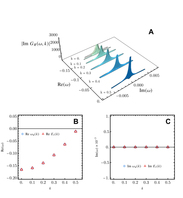
This general structure of the spectral function including the gap for $\omega_{-}\leq\omega\leq\omega_{+}$ can be seen in Figure 9. The data here and in the remainder of this section is computed for $\{\mu,q,m,\lambda\}=\{3/4,1.2,1/10,1\}$. Inside the gap (white area), the spectral weight of excitations is indeed zero to numerical accuracy except at the positions of the normal modes of the background fermions. The latter are computed directly from the solution of the background Dirac equation (green lines in Figure 9), as they cannot be seen numerically in the spectral function because they are infinitely long-living modes which show in the spectrum as Dirac delta peaks. Being infinitely narrow on the real axis, they can only be detected in the complex-$\omega$ plane. Representing schematically the normal mode located at $\omega_{\star}$ by Im$G(\omega=\text{Re}(\omega))=Z\delta(\omega-\omega_{\star})$ where $Z$ is the peak weight (wavefunction renormalization), we have, for complex $\omega$:

$$\imaginary G_{R}(\omega,k)=-Z\dfrac{\imaginary\omega-\imaginary\omega_{\star}}{\left(\real\omega-\real\omega_{\star}\right)^{2}+\left(\imaginary\omega-\imaginary\omega_{\star}\right)^{2}}~.$$

(39)

When $\real\omega=\real\omega_{\star}$, this simplifies to

$$\imaginary G_{R}(\omega,k)=-\dfrac{Z}{\imaginary\omega-\imaginary\omega_{\star}}~.$$

(40)

We check this picture against the numerics first in Figure 10 (A), where the absolute value of the spectral function in complex frequency plane shows the typical structure of a string of poles (for various momentum values) lying on the real axis. The relation (40) is then used to identify the dispersion relation of the pole $\omega_{\star}(k)$ by fitting $\imaginary G_{R}(\omega,k)$. We find, with no big surprise, a perfect agreement with the normal mode excitations $E_{1}(k)$ corresponding to the first electron band, as seen in Figure 10 (C) and (D). A similar picture is found for the first hole band $E_{-1}(k)$ and this yields the spectrum inside the gap, plotted in Figure 9.

In Figure 11 we compare the spectral function at finite $\mu$ for our regulated quantum electron star (blue data points) to the fermionic spectral function in a pure AdS₄ background with finite chemical potential, either with (green line) and without (red line) regulation by the confining scalar. The comparison is given at $k=0$ (left) and $k=1$ (right). The Dirac spectrum in AdS₄ is well-known Iqbal:2009fd:

$$G_{R}(\omega,k)=\begin{cases}\dfrac{2}{\omega^{2}-k^{2}}\dfrac{\Gamma(1/2-m)}{\Gamma(1/2+m)}\left[-\dfrac{i}{2}\left(\omega^{2}-k^{2}\right)\right]^{2m+1}\left[\omega\gamma^{0}-k\gamma^{1}\right]&\text{ if }\omega>k~,\\ \dfrac{2}{\omega^{2}-k^{2}}\dfrac{\Gamma(1/2-m)}{\Gamma(1/2+m)}\left[\dfrac{i}{2}\left(\omega^{2}-k^{2}\right)\right]^{2m+1}\left[\omega\gamma^{0}-k\gamma^{1}\right]&\text{ if }\omega<-k~.\\ \end{cases}$$

(41)

It has a conformal branch-cut at $\omega=k$ and a gap for $\omega^{2}<k^{2}$. For AdS₄ with finite electrostatic potential, one merely needs to replace $\omega\to\omega+\mu q$ in the previous expression. Adding confining potential by turning on the chirality-breaking flat scalar widens the gap to $(\omega+\mu q)^{2}<k^{2}+\lambda^{2}$; in particular the gap is open also at $k=0$. The rQES solution outside the gap exhibits qualitatively the same spectral function as that of the confined Dirac spectrum in pure AdS₄ but for renormalized IR values $\omega_{\mathrm{IR}},k_{\mathrm{IR}},\lambda_{\mathrm{IR}}$ given in (25). It is important to emphasize that none of the modes in this continuum are normalizable and thus do not contribute when building the bulk rQES, even when $\mu q$ is large enough that $\omega_{+}(k)<0$. This is guaranteed by our choice of UV boundary conditions.

By construction the confinement in our setup gives an AdS₄-to-AdS₄ solution. With the fully backreacted solution in hand we can also understand what the field theory dual describes. The confining regulator scale $\lambda$ gaps the field theory fermion spectral function. Considering then the RG flow from the IR emergent conformal field theory towards the UV, this means that as one increases the energy scale it takes a finite distance for occupiable fermion states to be encountered. This can also be seen in the band structure of Figure 6. At this scale the theory deforms away from the strict conformal theory up to the scale $\mu$ beyond which it is no longer energetically favorable to occupy more states. The flow up the RG then continues towards the UV AdS₄ fixed point.

In the more usual flow from the UV to the IR this is not a natural RG trajectory. The generic IR will not be a non-trivial conformal field theory. Nevertheless, within holography such AdS₄-to-AdS₄ domain walls are well-known. Especially in the search for the holographic dual of the holographic superconductor ground state, Horowitz and Roberts and independently Gubser and Rocha have found AdS₄-to-AdS₄ domain walls (in some cases with logarithmic corrections) in a finite parameter range HorowitzRob; Gubser:2008wz; the other solution found is the Lifshitz geometry. It was later understood that Lifshitz rather than an AdS₄ IR is the generic holographic superconductor ground state Gubser:2008wz; GubserNellore, but this is only seen with the inclusion of a stabilizing quartic potential.

In detail of course the solutions are different. The Horowitz-Roberts-Gubser-Rocha holographic superconductor ground states do not need an additional confining scalar. They can also be obtained classically without the need for a one-loop Hartree mean field. This is due to the fact that the bosonic field already couples quadratically to the electrostatic potential $A_{t}$. A fermion only couples linearly, but its one-loop contribution can couple at all orders. This is why for fermionic systems one needs to go to one-loop.

Given that the Horowitz-Roberts-Gubser-Rocha AdS₄-to-AdS₄ solutions do not need a confining potential, and that the more generic holographic superconductor Lifshitz solutions are known, it is a natural question why we do not try to remove the soft-confining regulator alltogether. There was in fact a concerted effort to do so several years ago Hartnoll:es; Leiden:2011; Leiden:2013, culminating in the QES model of McGreevy:2012; McGreevy:2013. The latter two articles show in detail how the presence of the gap and the discretized spectrum are crucial to construct any type of quantum fermionic backreacted solution, i.e. where one or a small finite number of radial modes are occupied. Any attempt to remove the confining potential results in a uncontrolled continuum spectrum.

It is precisely this insight that was the starting point for our confining potential. What we have furthermore shown, is that even then there are several severe technical hurdles to overcome to construct a converging fully backreacted confined quantum electron star solution. At the same time the general insight still holds. Our infrared boundary conditions crucially depend on the coupling to the scalar $\Phi(z)$ to extend the domain of existence of normalizable modes of AdS₄ all the way to $k=0$. The parameter $\lambda$, as we previously noted, acts as a momentum shift in this domain such that a mode at $k=0$ will behave as a mode at $k_{\mathrm{eff}}=\lambda$ and therefore normalizable modes with $|\omega+\mu q|<\lambda$ will be found. These can be populated and will condense in the bulk. Turning off the potential, even slowly, will invariably lead to a lack of normalizable modes at the lowest momenta and will bring us back to a situation similar to that of AdS₄.

References

- [1] Liza Huijse and Subir Sachdev. Fermi surfaces and gauge-gravity duality. Phys. Rev. D, 84:026001, 2011.
- [2] Hong Liu, John McGreevy, and David Vegh. Non-Fermi liquids from holography. Phys. Rev. D, 83:065029, 2011.
- [3] Mihailo Čubrović, Jan Zaanen, and Koenraad Schalm. String Theory, Quantum Phase Transitions and the Emergent Fermi-Liquid. Science, 325:439–444, 2009.
- [4] Thomas Faulkner, Hong Liu, John McGreevy, and David Vegh. Emergent quantum criticality, Fermi surfaces, and AdS(2). Phys. Rev. D, 83:125002, 2011.
- [5] Sean A. Hartnoll and Alireza Tavanfar. Electron stars for holographic metallic criticality. Phys. Rev. D, 83:046003, 2011.
- [6] V. Giangreco M. Puletti, S. Nowling, L. Thorlacius, and T. Zingg. Holographic metals at finite temperature. JHEP, 01:117, 2011.
- [7] Sean A. Hartnoll and Pavel Petrov. Electron star birth: A continuous phase transition at nonzero density. Phys. Rev. Lett., 106:121601, 2011.
- [8] Sean A. Hartnoll, Diego M. Hofman, and David Vegh. Stellar spectroscopy: Fermions and holographic Lifshitz criticality. JHEP, 08:096, 2011.
- [9] Mihailo Čubrović, Yan Liu, Koenraad Schalm, Ya-Wen Sun, and Jan Zaanen. Spectral probes of the holographic Fermi groundstate: dialing between the electron star and AdS Dirac hair. Phys. Rev. D, 84:086002, 2011.
- [10] Jan Zaanen, Ya-Wen Sun, Yan Liu, and Koenraad Schalm. Holographic Duality in Condensed Matter Physics. Cambridge Univ. Press, 2015.
- [11] Sean A. Hartnoll, Andrew Lucas, and Subir Sachdev. Holographic quantum matter. 12 2016.
- [12] Mariya V. Medvedyeva, Elena Gubankova, Mihailo Čubrović, Koenraad Schalm, and Jan Zaanen. Quantum corrected phase diagram of holographic fermions. JHEP, 12:025, 2013.
- [13] Subir Sachdev. A model of a Fermi liquid using gauge-gravity duality. Phys. Rev. D, 84:066009, 2011.
- [14] Andrea Allais, John McGreevy, and S. Josephine Suh. A quantum electron star. Phys. Rev. Lett., 108:231602, 2012.
- [15] Andrea Allais and John McGreevy. How to construct a gravitating quantum electron star. Phys. Rev. D, 88(6):066006, 2013.
- [16] Gary T. Horowitz and Matthew M. Roberts. Zero Temperature Limit of Holographic Superconductors. JHEP, 11:015, 2009.
- [17] Steven S. Gubser and Fabio D. Rocha. The gravity dual to a quantum critical point with spontaneous symmetry breaking. Phys. Rev. Lett., 102:061601, 2009.
- [18] Steven S. Gubser and Abhinav Nellore. Ground states of holographic superconductors. Phys. Rev. D, 80:105007, 2009.
- [19] Sean A. Hartnoll and Liza Huijse. Fractionalization of holographic Fermi surfaces. Class. Quant. Grav., 29:194001, 2012.
- [20] Christopher P. Herzog. A Holographic Prediction of the Deconfinement Temperature. Phys. Rev. Lett., 98:091601, 2007.
- [21] Guy F. de Teramond and Stanley J. Brodsky. Excited Baryons in Holographic QCD. AIP Conf. Proc., 1432(1):168–175, 2012.
- [22] Andreas Karch, Emanuel Katz, Dam T. Son, and Mikhail A. Stephanov. Linear confinement and AdS/QCD. Phys. Rev. D, 74:015005, 2006.
- [23] Zhen Fang, Danning Li, and Yue-Liang Wu. IR-improved Soft-wall AdS/QCD Model for Baryons. Phys. Lett. B, 754:343–348, 2016.
- [24] Norihiro Iizuka, Nilay Kundu, Prithvi Narayan, and Sandip P. Trivedi. Holographic Fermi and Non-Fermi Liquids with Transitions in Dilaton Gravity. JHEP, 01:094, 2012.
- [25] Lev Davidovich Landau and Evgeny Mikhailovich Lifshitz. Statistical Physics, Part 2: Theory of the Condensed State. Fizmatlit, 2004.
- [26] Steven S. Gubser, Fabio D. Rocha, and P. Talavera. Normalizable fermion modes in a holographic superconductor. JHEP, 10:087, 2010.
- [27] Frederik Denef, Sean A. Hartnoll, and Subir Sachdev. Quantum oscillations and black hole ringing. Phys. Rev. D, 80:126016, 2009.
- [28] Koji Hashimoto and Norihiro Iizuka. A Comment on Holographic Luttinger Theorem. JHEP, 07:064, 2012.
- [29] Nabil Iqbal, Hong Liu, and Mark Mezei. Semi-local quantum liquids. JHEP, 04:086, 2012.
- [30] Nabil Iqbal and Hong Liu. Real-time response in AdS/CFT with application to spinors. Fortsch. Phys., 57:367–384, 2009.
- [31] Gary Horowitz, Albion Lawrence, and Eva Silverstein. Insightful D-branes. JHEP, 07:057, 2009.