A novel formulation for the evolution of relativistic rotating stars 2022A novel formulation for the evolution of relativistic rotating stars–E

Hirotada Okawa Kotaro Fujisawa Thanks: E-mail: h.okawa@aoni.waseda.jp (WIAS) Affiliation: Waseda Institute for Advanced Study(WIAS), 1-21-1 Nishi-Waseda, Tokyo 169-0051, Japan Nobutoshi Yasutake Affiliation: Department of Physics, Graduate School of Science, University of Tokyo, Bunkyo-ku, Tokyo 113-0033, Japan Misa Ogata Affiliation: Physics Department, Chiba Institute of Technology, Chiba 275-0023, Japan Affiliation: Advanced Science Research Center, Japan Atomic Energy Agency, Tokai, Ibaraki 319-1195, Japan Yu Yamamoto Affiliation: Research Institute for Science and Engineering, Waseda University, Tokyo 169-8555, Japan Affiliation: Research Institute for Science and Engineering, Waseda University, Tokyo 169-8555, Japan Shoichi Yamada Affiliation: Research Institute for Science and Engineering, Waseda University, Tokyo 169-8555, Japan

Accepted XXX. Received YYY; in original form ZZZ

Abstract

We present a new formulation to construct numerically equilibrium configurations of rotating stars in general relativity. Having in mind the application to their quasi static evolutions, we adopt a Lagrangian formulation of our own devising, in which we solve force balance equations to seek for the positions of fluid elements assigned to the grid points, instead of the ordinary Eulerian formulation. Unlike previous works in the literature, we do not employ the first integral of the Euler equation, which is not obtained by an analytic integration in general. We assign a mass, specific angular momentum and entropy to each fluid element in contrast to the previous methods, in which the spatial distribution of the angular velocity or angular momentum is specified. Those distributions are determined after the positions of all fluid elements (or grid points) are derived in our formulation. We solve the large system of algebraic nonlinear equations that are obtained by discretizing the time-independent Euler and Einstein equations in the finite-elements method by using our new multi-dimensional root-finding scheme, named the W4 method. To demonstrate the capability of our new formulation, we construct some rotational configurations both barotropic and baroclinic. We also solve three evolutionary sequences that mimic the cooling, mass-loss, and mass-accretion as simple toy models.

Keywords:

stars: evolution – stars: rotation – stars: neutron – methods: numerical

1 Introduction

Neutron stars are promising compact objects to obtain the information on the equation of state of dense matter and investigate physics of strong gravity. The direct detections of gravitational waves from merging compact objects opened up a new window to access such information through the observation (Abbott et al. 2016; Abbott et al. 2017; Abbott et al. 2021). The neutron star is born in core-collapse supernova (for a review see, Janka et al. 2012; Burrows & Vartanyan 2021). A successful explosion leaves a proto-neutron star (PNS) in its supernova remnant, being decoupled from the expanding ejecta. At its birth, the PNS is initially hot and proton-rich (that is why it is called the proto-neutron star) and has a radius a few times larger than the typical size, $10\mathrm{km}$ , of neutron stars. Neutrinos and gravitational waves carry away energy from the PNS and cool it down to the neutron star on a diffusion timescale (a few tens of seconds) much longer than the dynamical timescale (Prakash et al. 1997).

It is quite numerically costly and impossible to follow the whole evolution of the PNS cooling by a dynamical simulation in multi-dimensions. Even recent core-collapse supernova simulations covered only the first $10$ seconds at most (Müller et al. 2019; Nakamura et al. 2019; Burrows et al. 2020; Nagakura et al. 2018). Thanks to the large separation of the two timescales, this long, quasi-static evolution of the PNS cooling may be approximated in a sequence of equilibrium configurations with gradually changing thermal and lepton contents. In fact, this was the common strategy in the past (Burrows & Lattimer 1986; Keil et al. 1996; Pons et al. 1999). Note that this was made possible by the fact that the Lagrangian formulation is easily employed in spherical symmetry.

It is not a trivial task, however, to adopt the same strategy in multi-dimensions for rotating stars. One of the big issues to be resolved is to devise a Lagrangian formulation that enables us to construct the equilibrium configurations of rotating stars. To the best of our knowledge, there has been no such method so far except for our own previous attempt in Newtonian gravity (Yasutake et al. 2015; Yasutake et al. 2016), in which we employ a triangular Lagrangian grid. It turns out, unfortunately, this scheme was neither robust nor very efficient. We hence need to build a new numerical scheme that is suitable for the study of the secular evolution of relativistic rotating stars such as PNSs to construct stationary rotating stars and solve two major issues: (i) to conceive a Lagrangian formulation in general relativity and (ii) its robust and efficient implementation¹¹ 1 A relativistic smoothed-particle-hydrodynamics formulation has been recently considered as dynamical problems in Rosswog & Diener 2021; Diener et al. 2022, whereas the Lagrange formulation as boundary value problems is not investigated in general relativity so far.. The latter is rather technical but turns out to be crucial as we explain later in detail.

The equilibrium configurations of relativistic rotating stars have been extensively investigated in the Eulerian formulation so far (see Paschalidis & Stergioulas 2017 for review): Rotating solutions in general relativity were discussed by Hartle 1967 and Butterworth & Ipser 1976, differentially rotating stars were successfully constructed by Komatsu et al. 1989b; Cook et al. 1992 ²² 2 This scheme was implemented in the RNS code by Stergioulas & Friedman 1995 which is now put in the public domain.; higher accuracy was attained by a spectral solver in Bonazzola et al. 1993 and Ansorg et al. 2002. More recent progresses now allow triaxial stars and magnetized stars (Uryu & Tsokaros 2012; Zhou et al. 2018; Uryu et al. 2019). Note, however, that all these works made two assumptions a priori: (i) the barotropic condition, i.e., the pressure depends only on the density and (ii) the rotation law that assumes a functional relation between specific angular momentum and angular velocity, i.e., $F=F(\Omega)$ (Komatsu et al. 1989b) or $\Omega=\Omega(F)$ (Uryu et al. 2017). Under these assumptions, one can analytically integrate the Euler equation and the main task is to solve the Einstein equations. Non-barotropic stars in general relativity have been also built, though. In general relativity, for example, Camelio et al. 2019 proposed a restrictive formulation by introducing $p-\Omega$ coordinates whereas there has been more works in the Newtonian gravity (Uryu & Eriguchi 1994; Uryu & Eriguchi 1995; Roxburgh 2006; Espinosa Lara & Rieutord 2007; Espinosa Lara & Rieutord 2013; Yasutake et al. 2015; Yasutake et al. 2016; Fujisawa 2015).

Based on the above Eulerian formulation of rotating stars, many authors have attempted to describe rotating PNSs (Goussard et al. 1997; Goussard et al. 1998; Sumiyoshi et al. 1999; Strobel et al. 1999; Villain et al. 2004; Camelio et al. 2016). Thanks to sophistication of numerical relativity with the rapid increase in computational power, on the other hand, some groups have started to use dynamical simulations (Camelio et al. 2019; Zhou et al. 2021; Fujibayashi et al. 2021) although they are limited to rather short periods. The dynamical simulations are put aside and the Eulerian formulation faces a difficulty when applied to the evolution of rotating stars: the angular momentum distribution in space is not known a priori (see assumption (ii) above) as a function of time even if there is no angular momentum transfer in the star. This is because in such a situation the specific angular momentum is conserved for the individual fluid element but the angular momentum distribution in space changes in time. This problem is automatically solved if one employs a Lagrangian formulation although it is highly nontrivial. That is our core idea in this paper.

The organization of the paper is as follows. In Sec. 2, we present this Lagrangian formulation of our devising. We then explain rather in detail how this formulation is implemented as a numerical scheme, since this part is actually crucial. We describe the models constructed in this paper to demonstrate the capability of our new method in Sec. 3 and show the results in Sec. 4. Finally, we summarize our findings and give future prospects in Sec. 5. Throughout this paper, geometrized units, i.e., $c=G=1$ are used unless otherwise noted.

2 Method

We start with a brief review of the ordinary numerical construction of axisymmetric rotating stars in general relativitic gravity in e.g. Komatsu et al. 1989a; Cook et al. 1992; Cook et al. 1994. Under axisymmetry and stationarity without circulation flows³³ 3 The metric ansatz for the case with circulation flows is discussed in Birkl et al. 2011. In this case, there are eight metric functions instead of four. the line element is given in general as

{\rm d}s^{2}=-N^{2}{\rm d}t^{2}+A^{-2}\left({\rm d}r^{2}+r^{2}{\rm d}\theta^{2}\right)+B^{-2}r^{2}\sin^{2}\theta\left({\rm d}\varphi-\omega{\rm d}t\right)^{2},\\

where $N(r,\theta),A(r,\theta),B(r,\theta),$ and $\omega(r,\theta)$ are functions of the radius and the zenith angle. Note that the metric components are not written in the exponential form (Komatsu et al. 1989b) but in the $3+1$ style in Bonazzola et al. 1993. The matter is assumed to be a perfect fluid and its energy momentum tensor is given as

\displaystyle T_{\mu\nu}=\left(\varepsilon+P\right)u_{\mu}u_{\nu}+Pg_{\mu\nu},

(1)

where $u^{\mu}$ is the 4-velocity and $\varepsilon\equiv\rho+\rho_{th}$ is the energy composed of the rest mass density $\rho$ and the internal energy density $\rho_{th}$ . The four-velocity is given as

\displaystyle u^{\mu}=\left(\frac{1}{N\sqrt{1-v^{2}}},0,0,\frac{\Omega}{N\sqrt{1-v^{2}}}\right)^{T},

(2)

where $v=\left(\Omega-\omega\right)N^{-1}B^{-1}r\sin\theta$ and $u^{\mu}u_{\mu}=-1$ . The angular velocity observed by the Zero Angular Momentum Observer (ZAMO) is denoted by $\Omega(r,\theta)$ .

Four metric functions $N(r,\theta),A(r,\theta),B(r,\theta)$ and $\omega(r,\theta)$ are determined by solving the Einstein equation $\displaystyle G_{\mu\nu}=8\pi T_{\mu\nu}$ . The energy-momentum conservation equation or the relativistic Euler equation is given by $\nabla_{\nu}T_{\mu}^{\ \nu}=0$ . The explicit differential forms of all these equations are presented in App. A. If the matter is barotropic, i.e., its pressure depends only on the density $P=P(\rho)$ , the equation of state (EOS) closes the system equation. If the matter is baroclinic, i.e., the pressure depends on another thermodynamic quantity, say the specific entropy $s$ as $P=P(\rho,s)$ ⁴⁴ 4 More generally, the pressure may depend on yet another thermodynamic quantity such as the electron fraction: $P=P(\rho,s,Y_{e})$ ., then the equation is augmented with the equation for energy. One often needs to solve the radiation transport equation as well (Pons et al. 1999).

There is a successful strategy common to the methods proposed in the literatures to numerically construct general relativistic rotating stars (see Paschalidis & Stergioulas 2017 for a recent review): (i) the Einstein equation is first solved for a given matter configuration; fixing the metric so obtained, we solve the Euler equation for density; replacing the matter configuration employed in the first step with the density distribution obtained in the second step, we iterate these two steps until the convergence is achieved as the self-consistent field method for Newtonian rotating stars in Hachisu 1986; (ii) the Euler equation is analytically integrated in advance, which is actually possible for the barotropic case: $\varepsilon=\varepsilon(P)$ or $P=P(\varepsilon)$ with $F(\Omega)=u^{t}u_{\varphi}$ where $F(\Omega)$ is an arbitrary function. In fact, the Euler equation under those assumptions:

\displaystyle\frac{1}{\varepsilon+P}{\rm d}P-{\rm d}\ln u^{t}+u^{t}u_{\varphi}{\rm d}\Omega=0,

(3)

leads to the first integral as follows:

\displaystyle\mathcal{H}(P)-\ln u^{t}+\mathcal{F}(\Omega)=\mathcal{C},

(4)

where $\mathcal{H}$ and $\mathcal{F}$ are given as

\displaystyle\mathcal{H}(P)\equiv\int^{P}\frac{{\rm d}P^{\prime}}{\varepsilon(P^{\prime})+P^{\prime}},\quad\mathcal{F}(\Omega)\equiv\int^{\Omega}F(\Omega^{\prime}){\rm d}\Omega^{\prime},

(5)

and $\mathcal{C}$ is an integration constant and may be determined at the pole. Although the methods based on this strategy have been successful in the numerical construction of a rotational configuration for a given functional form of angular velocity $F(\Omega)$ , they are not suited for the study of secular evolutions of rotating stars. There are two problems in fact: firstly, these methods are in principle applicable only to the barotropic case; secondly, the angular velocity distribution should be given in advance, which is normally impossible. The latter point will be understood if one considers the secular thermal evolution with the specific angular momentum being conserved in each fluid element. In fact, the spatial distribution of the angular velocity changes in time in this case even though there is no angular momentum transfer. This last point motivated us to develop a Lagrangian method in this paper, with which such a change of the angular velocity distribution can be automatically solved. Note also that it is not necessary to use the first integral in our formulation (see 34 and 35).

2.1 Lagrangian method

In the Eulerian formulation, one first introduces the coordinates rather arbitrarily according to the convenience in their applications; once chosen, they are unchanged; we then solve the density(or pressure) and the metric functions of the coordinates so that they should satisfy the Euler equation and the Einstein equation, respectively. As mentioned earlier, the angular velocity profile, or equivalently the angular momentum distribution should be given as input normally. It is also mentioned that the mass and angular momentum that characterizes a rotational star are normally obtained only after the solution is obtained.

In sharp contrast, in the Lagrangian formulation we solve the Euler equation to obrain the coordinates, which are attached to fluid elements. More specifically, assigning the mass, specific angular momentum and specific entropy to each fluid element⁵⁵ 5 The specific angular momentum and specific entropy hence regarded as functions of fluid elements. We may also give the electron fraction $Y_{e}$ ., we will look for the positions of fluid elements that satisfy the Euler equation. In so doing, the density is a functional of the coordinate configurations. The pressure at each fluid element is derived with the equation of state once the density is known there as the specific entropy is also known a priori. The spatial distribution of the angular velocity, or equivalently the angular momentum, is obtained once the coordinate configuration is determined. It should be apparent that the mass and angular momentum are automatically conserved in this formulation. In the following we will explain more in detail how these procedures are realized and implemented in the numerical construction of rotating stars.

2.1.1 Density in a Finite Element

Refer to caption — Figure 1: Schematic picture of finite elements. The circles denote the Lagrange nodes and the evaluation point for the Euler equation. Other physical variables are defined at the crosses and the Einstein equation is solved there.

In our brand new Lagrangian formulation of axisymmetric stars in permanent rotation, the starting point is to express the density in terms of the coordinates configuration. For its numerical realization on the finite-elements (FEs), we approximate each fluid element in the meridian section by a quadrilateral FE and assign mass $\Delta m$ , specific angular momentum $\Delta j$ , specific entropy $\Delta s$ , and electron fraction $\Delta Y_{e}$ , etc. The configuration of FE is specified by the coordinates $(x_{jk},y_{jk})$ , or specifically $(r_{jk},\theta_{jk})$ in axisymmetric stars, of its four corners as shown in Fig. 1 and its area may be calculated conveniently with the isoparametric formulation as follows (see, e.g., Bathe 2006). In this formulation, we introduce the natural coordinates $(\alpha,\beta)$ , $-1\geq\alpha,\beta\geq 1$ , which specify an arbitrary point in the FE as

	$\displaystyle x(\alpha,\beta)$	$\displaystyle=$	$\displaystyle\sum_{j=1}^{2}\sum_{k=1}^{2}\hat{N}_{j}(\alpha)\hat{N}_{k}(\beta)x_{jk},$
	$\displaystyle y(\alpha,\beta)$	$\displaystyle=$	$\displaystyle\sum_{j=1}^{2}\sum_{k=1}^{2}\hat{N}_{j}(\alpha)\hat{N}_{k}(\beta)y_{jk},$		(6)

where $\hat{N}_{j}(j=1,2)$ are called the shape function; $x_{jk}$ and $y_{jk}$ are the original coordinates at the four corners. Equation (6) is actually an interpolation formula and the linear shape functions are given as

\displaystyle\hat{N}_{1}(\alpha)=\frac{1-\alpha}{2},\quad\hat{N}_{2}(\alpha)=\frac{1+\alpha}{2}.

(7)

In App. B, we explain the basic idea underlying this formulation. The coordinate transformation from $(x,y)$ to $(\alpha,\beta)$ is characterized by the Jacobian matrix

\displaystyle J=\begin{pmatrix}\displaystyle\frac{\partial x}{\partial\alpha}&\displaystyle\frac{\partial y}{\partial\alpha}\\ &\\ \displaystyle\frac{\partial x}{\partial\beta}&\displaystyle\frac{\partial y}{\partial\beta}\end{pmatrix}.

(8)

For instance, the elements of which are given as

\displaystyle\frac{\partial x}{\partial\alpha}=\sum_{j=1}^{2}\sum_{k=1}^{2}\frac{{\rm d}\hat{N}_{j}}{{\rm d}\alpha}(\alpha)\hat{N}_{k}(\beta)x_{jk}.

(9)

Adopting $x_{jk}=r_{jk}^{3}/3$ and $y_{jk}=\cos\theta_{jk}$ in the current case, we define the volume of the FE in the flat space as

\displaystyle\Delta V=2\pi|\det J|.

(10)

By accounting for the curvature of the space, the baryonic density for the FE is given by

\displaystyle\bar{\rho}=\frac{\Delta m}{\sqrt{-g}\Delta V},

(11)

where the $g$ is the determinant of the spacetime metric. Since we evaluate the Einstein equation at each cell boundary as marked with crosses in Fig. 1, we need the densities at these boundaries. In this paper, they are given as a simple arithmetic mean of the densities for the adjascent FEs as $\rho_{jk}\equiv\left(\bar{\rho}_{jk}+\bar{\rho}_{jk-1}\right)/2$ . Note again that the density itself is the variable to be solved in the Eulerian formulation, whereas the coordinates are to be solved in the Lagrangian formulation.

2.1.2 Isoparametric interpolation and differentiation

In order to solve the Einstein and Euler equations in their differential forms, Eqs. (34)-(39), in the Lagrangian formulation, we need to evaluate not only the values of variables but also their derivatives at an arbitrary position. It is not a difficult task in the FE description. Since we need to evaluate second-order derivatives in the Einstein equation, we employ the second-order interpolation, in which we use quadratic shape functions and not the values of four but nine nearby points. Then the coordinates are expressed in terms of the natural coordinates $\alpha$ and $\beta$ as

	$\displaystyle x(\alpha,\beta)$	$\displaystyle=$	$\displaystyle\sum_{j=1}^{3}\sum_{k=1}^{3}\hat{M}_{j}(\alpha)\hat{M}_{k}(\beta)x_{jk},$		(12)
	$\displaystyle y(\alpha,\beta)$	$\displaystyle=$	$\displaystyle\sum_{j=1}^{3}\sum_{k=1}^{3}\hat{M}_{j}(\alpha)\hat{M}_{k}(\beta)y_{jk},\$		(13)

where the shape functions are given by

$\displaystyle\hat{M}_{1}(\alpha)$	$\displaystyle=$	$\displaystyle-\frac{\alpha}{2}(1-\alpha),$
$\displaystyle\hat{M}_{2}(\alpha)$	$\displaystyle=$	$\displaystyle(1+\alpha)(1-\alpha),$
$\displaystyle\hat{M}_{3}(\alpha)$	$\displaystyle=$	$\displaystyle\frac{\alpha}{2}(1+\alpha).$	(14)

We expand any function $\phi(x(\alpha,\beta),y(\alpha,\beta))$ with the same shape functions as

\displaystyle\phi(\alpha,\beta)

\displaystyle=

\displaystyle\sum_{j=1}^{3}\sum_{k=1}^{3}\hat{M}_{j}(\alpha)\hat{M}_{k}(\beta)\phi_{jk}.

(15)

It is straightforward to evaluate the derivatives of such a function with the derivatives of the shape functions:

$\displaystyle\frac{{\rm d}\hat{M}_{1}}{{\rm d}\alpha}(\alpha)$	$\displaystyle=$	$\displaystyle-\frac{1}{2}+\alpha,$
$\displaystyle\frac{{\rm d}\hat{M}_{2}}{{\rm d}\alpha}(\alpha)$	$\displaystyle=$	$\displaystyle-2\alpha,$
$\displaystyle\frac{{\rm d}\hat{M}_{3}}{{\rm d}\alpha}(\alpha)$	$\displaystyle=$	$\displaystyle\frac{1}{2}+\alpha.$	(16)

For instance, the first derivative with respect to $x$ can be obtained at any point as

\displaystyle\frac{\partial\phi}{\partial x}

\displaystyle=

\displaystyle\sum_{j,k=1}^{3}\left\{\frac{\partial\alpha}{\partial x}\frac{{\rm d}\hat{M}_{j}}{{\rm d}\alpha}\hat{M}_{k}+\frac{\partial\beta}{\partial x}\hat{M}_{j}\frac{{\rm d}\hat{M}_{k}}{{\rm d}\beta}\right\}\phi_{jk},

(17)

where the coefficients $\displaystyle\frac{\partial\alpha}{\partial x}$ and $\displaystyle\frac{\partial\beta}{\partial x}$ are computed straightforwardly from Eq. (12) as the coefficients of the inverse of the Jacobian matrix:

\displaystyle J^{-1}=\begin{pmatrix}\displaystyle\frac{\partial\alpha}{\partial x}&\displaystyle\frac{\partial\beta}{\partial x}\\ &\\ \displaystyle\frac{\partial\beta}{\partial y}&\displaystyle\frac{\partial\alpha}{\partial y}\end{pmatrix}=\frac{1}{\det J}\begin{pmatrix}\displaystyle\frac{\partial y}{\partial\beta}&\displaystyle-\frac{\partial y}{\partial\alpha}\\ &\\ \displaystyle-\frac{\partial x}{\partial\beta}&\displaystyle\frac{\partial x}{\partial\alpha}\end{pmatrix}.

(18)

2.1.3 Angular momentum

There are different definitions of specific angular momentum employed in the literature. For example, in the stationary and axisymmetric spacetime, the following specific angular momentum $\ell$ is introduced:

\displaystyle\ell=-\frac{u_{\varphi}}{u_{t}}=\frac{\left(\Omega-\omega\right)r^{2}\sin^{2}\theta}{N^{2}B^{2}+\omega\left(\Omega-\omega\right)r^{2}\sin^{2}\theta},

(19)

which is conserved along a stream line (Birkl et al. 2011). EoM, which can be written as

$\displaystyle\nabla^{\nu}T_{\mu\nu}$	$\displaystyle=$	$\displaystyle u^{\nu}\nabla_{\nu}\left[\left(\varepsilon+P\right)u_{\mu}\right]+\left(\varepsilon+P\right)u_{\mu}\nabla_{\nu}u^{\nu}+\nabla_{\mu}P$	(20)
	$\displaystyle=$	$\displaystyle u^{\nu}\nabla_{\nu}\left[\frac{\left(\varepsilon+P\right)}{\rho}u_{\mu}\rho\right]-\frac{\left(\varepsilon+P\right)}{\rho}u_{\mu}u^{\nu}\nabla_{\nu}\rho+\nabla_{\mu}P$
	$\displaystyle=$	$\displaystyle\rho u^{\nu}\nabla_{\nu}\left[\frac{\left(\varepsilon+P\right)}{\rho}u_{\mu}\right]+\nabla_{\mu}P=0,$

where the continuity equation is substituted, i.e. $\rho\nabla_{\nu}u^{\nu}=-u^{\nu}\nabla_{\nu}\rho$ , one finds for the spacetime with the asymptotically timelike and axial Killing vectors there are actually two quantities conserved along each stream line:

\displaystyle j_{t}=\frac{\varepsilon+P}{\rho}u_{t}\quad\mathrm{and}\quad j_{\varphi}=\frac{\varepsilon+P}{\rho}u_{\varphi}.

(21)

The specific angular momentum defined in Eq. (19) is nothing but the ratio of these two: $\ell=-j_{\varphi}/j_{t}$ Since we are interested in the formulation that can be applied to the evolution of rotating stars, the existence of the timeline Killing vector cannot be assumed. It should be noted that $j_{\varphi}$ is still conserved along the stream line even in this case as long as the spacetime is axisymmetric. We will hence employ this specific angular momentum and assume that it is conserved for each fluid element unless some mechanism to exchange angular momenta between fluid elements is in operation. Note, however, that the specific angular momentum $\ell$ is still very convenient from numerical point of view. In fact, it is simple to convert $\ell$ to the angular velocity $\Omega$

\displaystyle F\left(\Omega\right)=u^{t}u_{\varphi}=\frac{\ell}{1-\Omega\ell},

(22)

where $u_{\mu}u^{\mu}=-1$ and $u^{\varphi}=\Omega u^{t}$ .

2.2 Diagnostics

The following global quantities are useful for characterizing rotational equilibria. Following (Cook et al. 1992; Nozawa et al. 1998; Paschalidis & Stergioulas 2017), we define the baryon mass, proper mass and gravitational mass, respectively, as

$\displaystyle M_{b}$	$\displaystyle=$	$\displaystyle 2\pi\int\frac{\rho}{A^{2}B\sqrt{1-v^{2}}}r^{2}\sin\theta{\rm d}r{\rm d}\theta,$	(23)
$\displaystyle M_{p}$	$\displaystyle=$	$\displaystyle 2\pi\int\frac{\epsilon}{A^{2}B\sqrt{1-v^{2}}}r^{2}\sin\theta{\rm d}r{\rm d}\theta,$	(24)
$\displaystyle M$	$\displaystyle=$	$\displaystyle 2\pi\int\frac{1}{A^{2}B^{2}}\left[NB\left\{\frac{\left(\epsilon+P\right)\left(1+v^{2}\right)}{\left(1-v^{2}\right)}+2P\right\}\right.$	(25)
		$\displaystyle\left.\quad\quad\quad\quad\quad+2rv\omega\sin\theta\frac{\left(\epsilon+P\right)}{1-v^{2}}\right]r^{2}\sin\theta{\rm d}r{\rm d}\theta.$	(25)

On the other hand, the quantities employed to measure how fast the rotation is are the total angular momentum, rotational energy and gravitational energy, respectively, as

$\displaystyle J$	$\displaystyle=$	$\displaystyle 2\pi\int\frac{\left(\epsilon+P\right)v}{A^{2}B^{2}\left(1-v^{2}\right)}r^{3}\sin^{2}\theta{\rm d}r{\rm d}\theta,$	(26)
$\displaystyle T$	$\displaystyle=$	$\displaystyle 2\pi\int\frac{\left(\epsilon+P\right)v\Omega}{A^{2}B^{2}\left(1-v^{2}\right)}r^{3}\sin^{2}\theta{\rm d}r{\rm d}\theta,$	(27)
$\displaystyle W$	$\displaystyle=$	$\displaystyle M_{p}+T-M.$	(28)

2.2.1 Isoparametric integration

The integrations above are evaluated in each FE and summed as follows:

$\displaystyle S$	$\displaystyle\equiv$	$\displaystyle\int\!\!\!\!\int\!\!\!\phi(x,y){\rm d}x{\rm d}y=\int\!\!\!\!\int\!\!\!\phi\left(x(\alpha,\beta),y(\alpha,\beta)\right)\|\det J\|{\rm d}\alpha{\rm d}\beta$
	$\displaystyle=$	$\displaystyle\int\!\!\!\!\int\!\!\!\phi\left\|\frac{\partial x}{\partial\alpha}\frac{\partial y}{\partial\beta}-\frac{\partial x}{\partial\beta}\frac{\partial y}{\partial\alpha}\right\|{\rm d}\alpha{\rm d}\beta$
	$\displaystyle=$	$\displaystyle\sum_{i,j,k,l,m,n}^{2}\!\!\!\!\!\!\frac{\phi_{ij}x_{kl}y_{mn}}{4}\left\|(-1)^{k+n}\mathcal{N}_{im}\mathcal{N}_{jl}-(-1)^{m+l}\mathcal{N}_{ik}\mathcal{N}_{jn}\right\|,$

where the shape functions are analytically integrated over the ranges $-1\leq\alpha\leq 1$ and $-1\leq\beta\leq 1$ in advance as

\displaystyle\mathcal{N}_{ij}=\frac{1}{6}\begin{pmatrix}1&2\\ 2&1\end{pmatrix}.

(30)

2.3 Strategy to solve the system

To solve the whole system, we adopt the traditional iterative scheme (Hachisu 1986; Komatsu et al. 1989a). Specifically, it consists of two parts: (i) solving the Einstein equation, Eqs. (36)-(39), with the matter quantities unchanged and (ii) solving the Euler equation, Eqs. (34) and (35), with the metric functions fixed. Both equations in their differential forms are discretized on the FE grid and the resultant nonlinear algebraic equations are solved alternately until the changes in the solutions for both equations become smaller than certain values. As may be understood from the fact that many efforts have been made to choose a nice set of equations even in the Eulerian formulation, these nonlinear equations are difficult to solve and, it turns out, the original Newton-Raphson method does not work for our equations.

In order to tackle this problem, we deploy two new schemes of our own devising: (i) for the Einstein equation, the W4IX method is applied; as described in App. C, it is an extension of the original W4 method and requires only $\mathcal{O}(N^{2})$ calculations to obtain a solution, in contrast to $\mathcal{O}(N^{3})$ operations in the original W4 method with either the UL or LH decomposition (see Okawa et al. 2018; Fujisawa et al. 2019 for details); (ii) for the Euler equation on the other hand, we find that a particular iteration scheme dubbed the slice shooting is very powerful to obtain convergence; as demonstrated in App. D, the Jacobian matrix for the nonlinear force-balance equations in the $\theta$ -direction is especially ill-conditioned as the size of the matrix becomes bigger; we find it better to solve a single radial slice at a time with all the other slices fixed; we repeat this for all the slices, starting from the axis, proceeding to the equator and going back to the axis; this cycle is repeated until the convergence is obtained globally.

These two schemes turn out to be very successful. They are robust and also efficient and actually the key ingredients of our new formulation.

3 Models

In this section, we describe some models we employ in this paper to demonstrate the capability of our new method. As explained already, in this formulation we first assign the mass and specific angular momentum to the grid points and find their configuration that satisfies the Euler equation, or force-balance equations, as well as the spacetime metric that is consistent with the matter distribution by solving the Einstein equation. The spatial profiles of the density and angular velocity, respectively, are obtained from Eqs. (11) and (19), respectively, after the equilibrium configurations of the matter and spacetime are derived. Having an application to PNSs in mind, we also allocate the electron fraction to the Lagrange grid points.

The ultimate goal of this project is to study secular evolutions of relativistic rotating stars. The models are hence divided into two groups:

•

Stationary rotating stars constructed either with a barotropic EOS or with a baroclinic EOS and their accuracies investigated closely with a couple of diagnostic quantities; a comparison made with an Eulerian code,
•

mock evolutionary sequences of rotating stars considered for some scenarios: cooling, mass-loss, and mass-accretion; they are meant for demonstrations.

Each model is described more in detail below.

3.1 Stationary models

Here we adopt the so-called $j-$ const law (Komatsu et al. 1989b). This is actually the easiest case for our formulation, in which the specific angular momentum is assigned to the grid points and fixed. Then the angular velocity profile is derived after the equilibrium configuration is obtained. We begin with a barotropic EOS. In this case, as mentioned in introduction, we analytically obtain a first integral of the Euler equation, which gives for the present case the relation that the angular velocity should satisfy as

	$\displaystyle F(\Omega)$	$\displaystyle\equiv$	$\displaystyle u^{t}u_{\varphi}$
		$\displaystyle=$	$\displaystyle A_{c}^{2}(\Omega_{c}-\Omega)=\frac{(\Omega-\omega)r^{2}\sin^{2}\theta}{N^{2}B^{2}-(\Omega-\omega)^{2}r^{2}\sin^{2}\theta},$

where $A_{c}$ and $\Omega_{c}$ are constants. Once the metric functions are obtained, we can derive the angular velocity as a function of $r$ and $\theta$ , which should be compared with the profile derived directly from the equilibrium configuration. Note that this relation is reduced to a cylindrical rotation law in the non-relativistic limit.

As mentioned repeatedly, our new formulation can accommodate any EOS, which may depend not only on density and entropy but also on other quantities such as electron fraction and mass fractions of various nuclei. In this paper, we employ a polytropic type of EOS for simplicity:

\displaystyle P(\rho,s(r,\theta))=K(r,\theta)\rho^{1+\frac{1}{N}},

(32)

where $N$ is the polytropic index; note that $K$ , which is normally a constant and is a function of entropy, is assumed here to be a function of $r$ and $\theta$ as

\displaystyle K(r,\theta)\equiv\hat{K}\left(K_{0}+\epsilon_{1}\frac{r^{2}}{R_{e}^{2}}\sin^{2}\theta+\epsilon_{2}\frac{r^{2}}{R_{e}^{2}}\cos^{2}\theta+\epsilon_{3}\frac{r^{2}-R_{e}^{2}}{R_{e}^{2}}\right),

(33)

where $R_{e}$ is the equatorial surface radius of the star; $K_{0},\epsilon_{1},\epsilon_{2},\epsilon_{3}$ are constants. The polytropic index is set to $N=1$ in the following. For the stationary models, we set $K_{0}=1$ as well. Note that we use the geometrical unit $c=G=1$ and put $\hat{K}=1$ in actual calculations following (Cook et al. 1992).

It should be apparent that the baroclinicity is introduced by the non-constancy of $K$ in this EOS. In fact we set all $\epsilon$ ’s to $0$ for the barotropic case above. In the baroclinic case, we solve the Einstein and Euler equations keeping the specific angular momentum attached to grid points the same as that of the reference model. We have to update the value of $K$ at each grid point according to its current position and Eq. (32).

Code	$N_{r}\times N_{\theta}$	$\rho_{c}$	$r_{p}/r_{e}$	$M$	$M_{b}$
our code	$32\times 17$	$0.0562$	$0.874$	$0.0958$	$0.100$
RNS code	$65\times 129$	$0.0562$	$0.870$	$0.0967$	$0.101$

Table 1: Parameters for comparison with the public RNS code by Stergioulas & Friedman 1995.

3.2 Evolutionary models

In its real evolution, the PNS cools down through neutrino emissions and experiences a sequence of quasi-equilibrium during a period of about a minute. If it rotates as normally expected, these are rotational equilibria with different thermal and lepton contents but with the same specific angular momentum if the angular momentum transfer is negligible. To understand such secular evolutions of PNS, it is necessary to construct a series of configurations of rotational equilibria and to compute the neutrino transfer on top of them. The main aim of this paper is to provide a new numerical tool to treat the first step, i.e., the building of a sequence of rotational equilibria that are supposed to represent the secular evolution of the rotating PNS. The purpose of the models considered here is to demonstrate the capability of our new Lagrangian formulation in full general relativity with some mock evolutions. The application of the method to more realistic evolutions is currently underway and will be presented elsewhere in the near future.

For the mock evolutions, we consider the following three scenarios. We stress that in our formulation we need to give an angular velocity distribution only at the beginning of each sequence and it is automatically derived thereafter during the evolution⁶⁶ 6 We need to specify the specific angular momentum of accreting matter in scenario (iii)..

1.

Cooling model: The first model is intended to mimic a cooling evolution by the neutrino emission, in which the PNS shrinks as the thermal energy is carried away by neutrinos. In realistic simulations (Pons et al. 1999; Villain et al. 2004), we need to calculate the entropy (and electron fraction) evolution with the neutrino transfer. For the demonstrative purpose here, it suffices to prescribe the time-dependence of $K$ in the Polytropic EOS by hand so that it should mimic the cooling.
2.

Wind model: The second model is to mimic the evolution of a rotating star via the mass-loss from the surface as a wind. The neutrino-driven wind from the PNS has been considered in Meyer et al. 1992; Witti et al. 1992; Woosley et al. 1994; Otsuki et al. 2000; Sumiyoshi et al. 2000; Terasawa et al. 2001; Wanajo et al. 2001; Panov & Janka 2009. Such a stellar wind carries not only mass but also angular momentum. In this toy model, we emulate the mass-loss process by taking a certain fraction of mass and angular momentum away from the grid points near the stellar surface at a certain rate.
3.

Accretion model: In the third model, we consider the evolution induced by the accretion of matter, the process opposite to the one in model (ii). Recent core-collapse supernova simulations (e.g. Müller et al. 2019; Burrows et al. 2019; Nakamura et al. 2019; Janka et al. 2021) indicate that asymmetric accretion flows continue to exist for a few seconds after the revival of a stalled shock wave and may affect the angular momentum of PNS (Blondin & Mezzacappa 2007; Fernández 2010; Wongwathanarat et al. 2013; Guilet & Fernández 2014; Kazeroni et al. 2017). In this model, we simply increase the masses and angular momenta of the grid points near the surface at a certain rate, to consider the spin-up evolution of PNS.

Model	Number of Grids( $N_{r}\times N_{\theta}$ )	$R_{p}/R_{e}$	$M_{b}$	$M$	$J$	$T/\|W\|$	GRV
Reference	$32\times 17$	$0.893$	$0.0999$	$0.0961$	$3.91\times 10^{-3}$	$6.02\times 10^{-2}$	$0.976\times 10^{-3}$
Middle-Resolution	$16\times 9$	$0.891$	$0.0999$	$0.0958$	$3.77\times 10^{-3}$	$5.61\times 10^{-2}$	$4.51\times 10^{-2}$
Low-Resolution	$8\times 5$	$0.885$	$0.0986$	$0.0950$	$1.93\times 10^{-3}$	$3.66\times 10^{-2}$	$1.22\times 10^{-1}$
EOS-a	$32\times 17$	$0.874$	$0.0994$	$0.0946$	$3.95\times 10^{-3}$	$5.14\times 10^{-2}$	$2.07\times 10^{-3}$
EOS-b	$32\times 17$	$0.911$	$0.100$	$0.0956$	$3.87\times 10^{-3}$	$5.34\times 10^{-2}$	$3.78\times 10^{-3}$
EOS-c	$32\times 17$	$0.894$	$0.0999$	$0.0954$	$3.91\times 10^{-3}$	$5.32\times 10^{-2}$	$2.91\times 10^{-3}$
Middle-Rotation	$32\times 17$	$0.812$	$0.0997$	$0.0951$	$5.79\times 10^{-3}$	$9.88\times 10^{-2}$	$6.75\times 10^{-3}$
Cooling	$32\times 17$	$0.895$	$0.0989$	$0.0955$	$3.85\times 10^{-3}$	$6.47\times 10^{-2}$	$8.02\times 10^{-3}$
Wind	$32\times 17$	$0.890$	$0.0980$	$0.0943$	$3.80\times 10^{-3}$	$5.90\times 10^{-2}$	$7.27\times 10^{-3}$
Accretion	$32\times 17$	$0.895$	$0.102$	$0.0981$	$4.22\times 10^{-3}$	$6.71\times 10^{-2}$	$4.74\times 10^{-3}$

Table 2: List of models: The first column shows the model name. The second corresponds to the number of grid points, followed by the ratio of the polar radius to the equatorial radius of the star, the baryon mass, the gravitational mass, the total angular momentum,

T/|W|

, and relativistic Virial relation (GRV2) in Nozawa et al. 1998.

4 Results

In this section, starting from the comparison of our solution with that by the public RNS code, we show barotropic stationary models and baroclinic stationary models, followed by the three mock evolutionary models, namely, cooling, wind, and accretion models.

4.1 Uniformly rotating stars

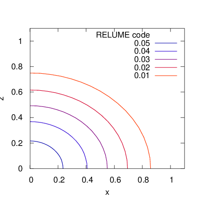
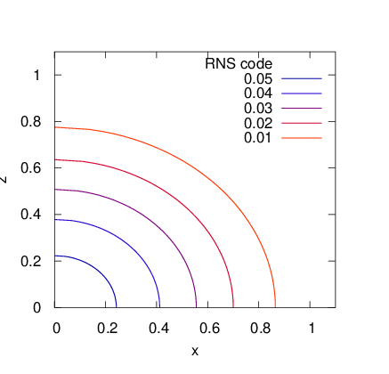
Fortunately, it is possible to directly compare our result in the Lagrange formulation with the solution given by the well-known public RNS code for uniformly-rotating stars (Stergioulas & Friedman 1995). In Fig. 2, we show the density contour of a uniformly rotating star (a) by our new code in the Lagrangian formulation and (b) by the RNS code in the literature. Since the input parameters to construct equilibrium configurations are different in the Eurelian and Lagrangian formulations, we finetune those parameters to obtain almost the same rotating star as possible as we can, which the global quantities are compared in Table 1. Note also that the relativistic Virial relation of our solution is $8.94\times 10^{-3}$ , which indicates the accuracy of solutions (Nozawa et al. 1998).

4.2 Stationary models with barotropic EOS

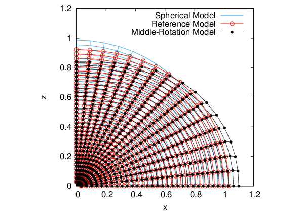
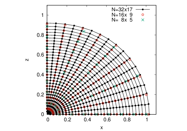
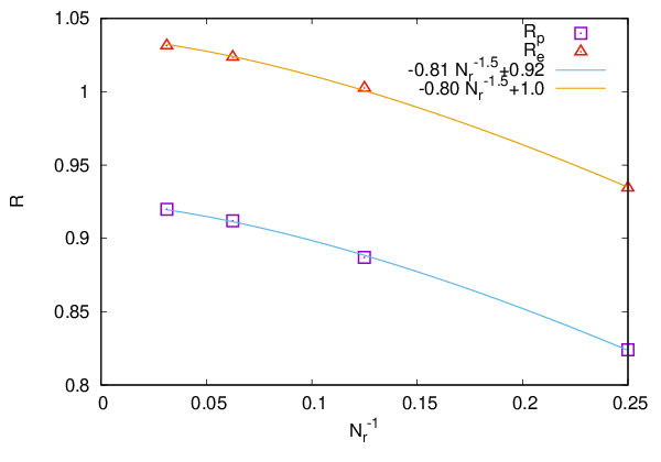
We first focus on the barotropic rotating stars with $\epsilon_{1}=\epsilon_{2}=\epsilon_{3}=0$ and the EOS described in Eq. (32). As the angular velocity is faster, the star is oblater. In Fig. 3, the spherical and middle-rotation models are compared with the reference model. Furthermore, the resolution dependence is investigated in Fig. 4. The solution converges as the resolution increases. As shown in Fig. 4 (b), the convergence order is 1.5, which is expected because we employ the first-order FE scheme to calculate the baryon density while we use the second-order FE scheme to evaluate the derivatives. In this work, we adopt the model with $N_{r}\times N_{\theta}=32\times 17$ as the reference model for other computations. Note that our solutions with the resolution $(N_{r}\times N_{\theta}=32\times 17)$ typically has the Virial relation of $\mathcal{O}(10^{-3})$ in Table 2.

4.3 Stationary models with baroclinic EOS

Next, we investigate the effect of the baroclinicity on the equilibrium configuration of rotating stars. In Fig. 5, we observe the baroclinic feature, which is the misalignment between the pressure and density gradients as Figs. 5 (b), (d) and (f). To clearly see the difference between the barotropic and baroclinic models, we show the angular velocity as a function of the specific angular momentum in Figs. 5 (a), (c) and (e) as shown in Camelio et al. 2019. Isentropic rotating stars in general relativity satisfy the condition that is expressed as the black solid line by $\ell=\ell(\Omega)$ from Eqs. (22) and (). Although a type of shellular rotation has been considered as the initial rotation in core-collapse supernova simulations (e.g. Yamada & Sato 1994; Harada et al. 2019; Iwakami et al. 2021), the self-consistent stationary solutions with baroclinicity have been obtained only in the Newtonian gravity so far (Roxburgh 2006; Fujisawa 2015). We first obtain such a self-consistent stationary solution with baroclinicity in general relativity in Fig. 5 (d). Since the model (EOS-c) does not satisfy the Høiland criterion in the Newtonian limit and may be dynamically unstable (Tassoul 1978), we leave the detailed investigation on the dynamical stability for baroclinic rotating stars in the future study.

4.4 Cooling of rotating stars

As an evolution test by cooling, we vary the polytropic constant $K_{0}$ keeping the other parameters constant. In Fig. 6 (a), we compare the cooling model ( $K_{0}=0.95$ ) with the reference model ( $K_{0}=1$ ). Rotating stars shrink for nonlinear balance equations between the pressure and the gravity to be satisfied. We emphasize that we do not impose any rotational law explicitly but keep the specific angular momentum $j_{\varphi}$ of each FE. As mentioned, barotropic rotating stars satisfy the condition $\ell=\ell(\Omega)$ between $\ell$ and $\Omega$ for any equilibria configurations. In fact, Fig. 6 (b) shows that the angular velocity of the cooling model as a function of the specific angular momentum is still expressed as the line, which is highly non-trivial in this Lagrangian formulation.

4.5 Wind and accretion models

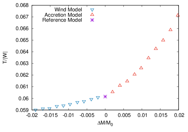
For the wind model, we assume the mass-loss from the outer layer of rotating stars. Specifically, we decrease the specific masses of the outer two layers by hand as a toy model and compute a new equilibrium configuration. For the accretion model, on the other hand, we assume the accreting matter that is composed of both the $5\%$ mass and angular momentum of outer layers of rotating stars for simplicity. By the mass-loss or accretion, the total mass and total angular momentum are expected to change accordingly. In Fig. 7, we show $T/|W|$ as a function of the mass change.

5 Conclusions

We have proposed a new scheme to construct the equilibrium configuration of general relativistic rotating stars in the Lagrangian formulation, which maintains the mass and angular momentum automatically when no angular momentum transfer exists, in contrast to the Eulerian formulation. We employed the traditional iterative scheme (Hachisu 1986) to solve the whole system derived from discretizing the Einstein and Euler equations on the finite-elements grid, which consists of two new schemes of our own devising: for the Einstein equation, the W4IX method in App. C is applied and for the Euler equation, the slice-shooting scheme is adopted in App. D.

Our formulation does need an angular velocity profile only at initial and employ any equation of state. It enables us to find the evolutionary sequence by keeping the mass, specific angular momentum, specific entropy, electron fraction and mass fraction of various nuclei. In order to demonstrate the capability of our new formulation, we first compare our result of uniformly-rotating stars with that given by the public RNS code (Stergioulas & Friedman 1995). Next, we present the stationary rotating stars with the barotropic and baroclinic equations of state. Finally, we consider the mock evolutionary sequences for cooling, wind and accretion as toy models and show those results.

In this paper, we adopt simple models for finding the evolutionary sequence, since our focus is on the way of constructing the equilibrium configuration in the Lagrangian formulation. The application of our new method to more realistic situations is currently underway and will be presented in the near future.

Acknowledgements

We would like to thank K-i. Maeda for helpful comments. This work was supported by JSPS KAKENHI Grant Number 20K03951, 20K03953, 20K14512, 20H04728, 20H04742, and by Waseda University Grant for Special Research Projects(Project Number: 2019C-640).

Data Availability

The data underlying this paper will be available from the corresponding author on reasonable request.

References

Abbott et al. (2016) Abbott B. P., et al., 2016, Phys. Rev. Lett., 116, 061102
Abbott et al. (2017) Abbott B. P., et al., 2017, Phys. Rev. Lett., 119, 161101
Abbott et al. (2021) Abbott R., et al., 2021, The Astrophysical Journal Letters, 915, L5
Ansorg et al. (2002) Ansorg M., Kleinwächter A., Meinel R., 2002, A&A, 381, L49
Bathe (2006) Bathe K.-J., 2006, Finite element procedures. Klaus-Jurgen Bathe
Birkl et al. (2011) Birkl R., Stergioulas N., Muller E., 2011, Phys. Rev. D, 84, 023003
Blondin & Mezzacappa (2007) Blondin J. M., Mezzacappa A., 2007, Nature, 445, 58
Bonazzola et al. (1993) Bonazzola S., Gourgoulhon E., Salgado M., Marck J. A., 1993, A&A, 278, 421
Burrows & Lattimer (1986) Burrows A., Lattimer J. M., 1986, Astrophys. J., 307, 178
Burrows & Vartanyan (2021) Burrows A., Vartanyan D., 2021, Nature, 589, 29
Burrows et al. (2019) Burrows A., Radice D., Vartanyan D., Nagakura H., Skinner M. A., Dolence J. C., 2019, Monthly Notices of the Royal Astronomical Society, 491, 2715
Burrows et al. (2020) Burrows A., Radice D., Vartanyan D., Nagakura H., Skinner M. A., Dolence J., 2020, Mon. Not. Roy. Astron. Soc., 491, 2715
Butterworth & Ipser (1976) Butterworth E. M., Ipser J. R., 1976, ApJ, 204, 200
Camelio et al. (2016) Camelio G., Gualtieri L., Pons J. A., Ferrari V., 2016, Phys. Rev. D, 94, 024008
Camelio et al. (2019) Camelio G., Dietrich T., Marques M., Rosswog S., 2019, Phys. Rev. D, 100, 123001
Cook et al. (1992) Cook G. B., Shapiro S. L., Teukolsky S. A., 1992, ApJ, 398, 203
Cook et al. (1994) Cook G. B., Shapiro S. L., Teukolsky S. A., 1994, Astrophys. J., 422, 227
Diener et al. (2022) Diener P., Rosswog S., Torsello F., 2022
Espinosa Lara & Rieutord (2007) Espinosa Lara F., Rieutord M., 2007, A&A, 470, 1013
Espinosa Lara & Rieutord (2013) Espinosa Lara F., Rieutord M., 2013, A&A, 552, A35
Fernández (2010) Fernández R., 2010, ApJ, 725, 1563
Fujibayashi et al. (2021) Fujibayashi S., Takahashi K., Sekiguchi Y., Shibata M., 2021, ] 10.3847/1538-4357/ac10cb
Fujisawa (2015) Fujisawa K., 2015, MNRAS, 454, 3060
Fujisawa et al. (2019) Fujisawa K., Okawa H., Yamamoto Y., Yamada S., 2019, Astrophys. J., 872, 155
Gourgoulhon et al. (2015) Gourgoulhon E., Bejger M., Mancini M., 2015, Journal of Physics: Conference Series, 600, 012002
Goussard et al. (1997) Goussard J.-O., Haensel P., Zdunik J. L., 1997, Astron. Astrophys., 321, 822
Goussard et al. (1998) Goussard J. O., Haensel P., Zdunik J. L., 1998, Astron. Astrophys., 330, 1005
Guilet & Fernández (2014) Guilet J., Fernández R., 2014, Mon. Not. Roy. Astron. Soc., 441, 2782
Hachisu (1986) Hachisu I., 1986, ApJS, 61, 479
Harada et al. (2019) Harada A., Nagakura H., Iwakami W., Okawa H., Furusawa S., Matsufuru H., Sumiyoshi K., Yamada S., 2019, Astrophys. J., 872, 181
Hartle (1967) Hartle J. B., 1967, ApJ, 150, 1005
Hirai et al. (2016) Hirai R., Nagakura H., Okawa H., Fujisawa K., 2016, Phys. Rev. D, 93, 083006
Iwakami et al. (2021) Iwakami W., et al., 2021
Janka et al. (2012) Janka H.-T., Hanke F., Hüdepohl L., Marek A., Müller B., Obergaulinger M., 2012, Progress of Theoretical and Experimental Physics, 2012
Janka et al. (2021) Janka H.-T., Wongwathanarat A., Kramer M., 2021
Kazeroni et al. (2017) Kazeroni R., Guilet J., Foglizzo T., 2017, Mon. Not. Roy. Astron. Soc., 471, 914
Keil et al. (1996) Keil W., Janka H. T., Muller E., 1996, Astrophys. J. Lett., 473, L111
Komatsu et al. (1989a) Komatsu H., Eriguchi Y., Hachisu I., 1989a, MNRAS, 237, 355
Komatsu et al. (1989b) Komatsu H., Eriguchi Y., Hachisu I., 1989b, MNRAS, 239, 153
Meyer et al. (1992) Meyer B. S., Mathews G. J., Howard W. M., Woosley S. E., Hoffman R. D., 1992, Astrophys. J., 399, 656
Müller et al. (2019) Müller B., et al., 2019, Mon. Not. Roy. Astron. Soc., 484, 3307
Nagakura et al. (2018) Nagakura H., et al., 2018, Astrophys. J., 854, 136
Nakamura et al. (2019) Nakamura K., Takiwaki T., Kotake K., 2019, Publ. Astron. Soc. Jap., 71, Publications of the Astronomical Society of Japan, Volume 71, Issue 5, October 2019, 98, https://doi.org/10.1093/pasj/psz080
Nozawa et al. (1998) Nozawa T., Stergioulas N., Gourgoulhon E., Eriguchi Y., 1998, Suppl
Okawa et al. (2018) Okawa H., Fujisawa K., Yamamoto Y., Hirai R., Yasutake N., Nagakura H., Yamada S., 2018
Otsuki et al. (2000) Otsuki K., Tagoshi H., Kajino T., Wanajo S.-y., 2000, Astrophys. J., 533, 424
Panov & Janka (2009) Panov I. V., Janka H. T., 2009, Astron. Astrophys., 494, 829
Paschalidis & Stergioulas (2017) Paschalidis V., Stergioulas N., 2017, Living Rev. Rel., 20, 7
Pons et al. (1999) Pons J. A., Reddy S., Prakash M., Lattimer J. M., Miralles J. A., 1999, Astrophys. J., 513, 780
Prakash et al. (1997) Prakash M., Bombaci I., Prakash M., Ellis P. J., Lattimer J. M., Knorren R., 1997, Phys. Rept., 280, 1
Press et al. (1992) Press W. H., Teukolsky S. A., Vetterling W. T., Flannery B. P., 1992, Numerical Recipes in FORTRAN: The Art of Scientific Computing
Rosswog & Diener (2021) Rosswog S., Diener P., 2021, Class. Quant. Grav., 38, 115002
Roxburgh (2006) Roxburgh I. W., 2006, A&A, 454, 883
Stergioulas & Friedman (1995) Stergioulas N., Friedman J. L., 1995, ApJ, 444, 306
Strobel et al. (1999) Strobel K., Schaab C., Weigel M. K., 1999, Astron. Astrophys., 350, 497
Sumiyoshi et al. (1999) Sumiyoshi K., Ibáñez J. M., Romero J. V., 1999, A&AS, 134, 39
Sumiyoshi et al. (2000) Sumiyoshi K., Suzuki H., Otsuki K., Terasawa M., Yamada S., 2000, Publ. Astron. Soc. Jap., 52, 601
Tassoul (1978) Tassoul J.-L., 1978, Theory of rotating stars
Terasawa et al. (2001) Terasawa M., Sumiyoshi K., Kajino T., Mathews G. J., Tanihata I., 2001, Astrophys. J., 562, 470
The Sage Developers (2019) The Sage Developers 2019, SageMath, the Sage Mathematics Software System (Version 8.6.0)
Uryu & Eriguchi (1994) Uryu K., Eriguchi Y., 1994, MNRAS, 269, 24
Uryu & Eriguchi (1995) Uryu K., Eriguchi Y., 1995, MNRAS, 277, 1411
Uryu & Tsokaros (2012) Uryu K., Tsokaros A., 2012, Phys. Rev. D, 85, 064014
Uryu et al. (2017) Uryu K., Tsokaros A., Baiotti L., Galeazzi F., Taniguchi K., Yoshida S., 2017, Phys. Rev. D, 96, 103011
Uryu et al. (2019) Uryu K., Yoshida S., Gourgoulhon E., Markakis C., Fujisawa K., Tsokaros A., Taniguchi K., Eriguchi Y., 2019, Phys. Rev. D, 100, 123019
Villain et al. (2004) Villain L., Pons J. A., Cerda-Duran P., Gourgoulhon E., 2004, Astron. Astrophys., 418, 283
Wanajo et al. (2001) Wanajo S., Kajino T., Mathews G. J., Otsuki K., 2001, Astrophys. J., 554, 578
Witti et al. (1992) Witti J., Janka H. T., Takahashi K., Hillebrandt W., 1992.
Wongwathanarat et al. (2013) Wongwathanarat A., Janka H. T., Mueller E., 2013, Astron. Astrophys., 552, A126
Woosley et al. (1994) Woosley S. E., Wilson J. R., Mathews G. J., Hoffman R. D., Meyer B. S., 1994, Astrophys. J., 433, 229
Yamada & Sato (1994) Yamada S., Sato K., 1994, ApJ, 434, 268
Yasutake et al. (2015) Yasutake N., Fujisawa K., Yamada S., 2015, MNRAS, 446, L56
Yasutake et al. (2016) Yasutake N., Fujisawa K., Yamada S., 2016, Mon. Not. Roy. Astron. Soc., 463, 3705
Zhou et al. (2018) Zhou E., Tsokaros A., Rezzolla L., Xu R., Uryū K., 2018, Phys. Rev. D, 97, 023013
Zhou et al. (2021) Zhou E., Kiuchi K., Shibata M., Tsokaros A., Uryu K., 2021, Phys. Rev. D, 103, 123011

Appendix A Explicit differential forms of Euler and Einstein equations

In this appendix, we describe the equations that we solve in our formulation. To obtain the field equations below, we use SageMath by The Sage Developers 2019 and SageManifolds packages by Gourgoulhon et al. 2015. The first order differential equations in the radial and polar angle directions from the Euler equation yield

	$\displaystyle 0=F_{r}$	$\displaystyle\equiv$	$\displaystyle\frac{(\Omega-\omega)^{2}r^{2}\sin^{2}\theta-N^{2}B^{2}}{P+\varepsilon}\frac{\partial P}{\partial r}-NB^{2}\frac{\partial N}{\partial r}-\frac{(\Omega-\omega)^{2}r^{2}\sin^{2}\theta}{B}\frac{\partial B}{\partial r}-\frac{(\Omega-\omega)r^{2}\sin^{2}\theta}{B}\frac{\partial\omega}{\partial r}+(\Omega-\omega)^{2}r\sin^{2}\theta,$		(34)
	$\displaystyle 0=F_{\theta}$	$\displaystyle\equiv$	$\displaystyle\frac{(\Omega-\omega)^{2}r^{2}\sin^{2}\theta-N^{2}B^{2}}{P+\varepsilon}\frac{\partial P}{\partial\theta}-NB^{2}\frac{\partial N}{\partial\theta}-\frac{(\Omega-\omega)^{2}r^{2}\sin^{2}\theta}{B}\frac{\partial B}{\partial\theta}-\frac{(\Omega-\omega)r^{2}\sin^{2}\theta}{B}\frac{\partial\omega}{\partial\theta}+(\Omega-\omega)^{2}r^{2}\sin\theta\cos\theta.$		(35)

As for the Einstein equation, among non-trivial components, we choose the following four second-order differential equations:

$\displaystyle E_{tt}$	$\displaystyle\equiv$	$\displaystyle G_{tt}-\frac{8\pi G}{c^{4}}T_{tt}$	(36)
	$\displaystyle=$	$\displaystyle\frac{A^{2}\omega^{2}\sin^{2}\theta}{NB^{2}}\left(r^{2}\frac{\partial^{2}N}{\partial r^{2}}+\frac{\partial^{2}N}{\partial\theta^{2}}\right)+\left(\frac{N^{2}A}{r^{2}}-\frac{A\omega^{2}\sin^{2}\theta}{B^{2}}\right)\left(r^{2}\frac{\partial^{2}A}{\partial r^{2}}+\frac{\partial^{2}A}{\partial\theta^{2}}\right)+\frac{N^{2}A^{2}}{r^{2}B^{2}}\left(r^{2}\frac{\partial^{2}B}{\partial r^{2}}+\frac{\partial^{2}B}{\partial\theta^{2}}\right)$
		$\displaystyle-\frac{A^{2}\omega\sin^{2}\theta}{B^{2}}\left(r^{2}\frac{\partial^{2}\omega}{\partial r^{2}}+\frac{\partial^{2}\omega}{\partial\theta^{2}}\right)+\frac{A^{2}\omega\sin^{2}\theta}{NB^{2}}\left(r^{2}\frac{\partial N}{\partial r}\frac{\partial\omega}{\partial r}+\frac{\partial N}{\partial\theta}\frac{\partial\omega}{\partial\theta}\right)+\frac{3A^{2}\omega\sin^{2}\theta}{B^{3}}\left(r^{2}\frac{\partial B}{\partial r}\frac{\partial\omega}{\partial r}+\frac{\partial B}{\partial\theta}\frac{\partial\omega}{\partial\theta}\right)$
		$\displaystyle-\left(\frac{N^{2}}{r^{2}}-\frac{\omega^{2}\sin^{2}\theta}{B^{2}}\right)\left\{r^{2}\left(\frac{\partial A}{\partial r}\right)^{2}+\left(\frac{\partial A}{\partial\theta}\right)^{2}\right\}-\frac{2N^{2}A^{2}}{r^{2}B^{2}}\left\{r^{2}\left(\frac{\partial B}{\partial r}\right)^{2}+\left(\frac{\partial B}{\partial\theta}\right)^{2}\right\}-\left(\frac{A^{2}\sin^{2}\theta}{4B^{2}}+\frac{3r^{2}\omega^{2}\sin^{4}\theta}{4N^{2}B^{4}}\right)\left\{r^{2}\left(\frac{\partial\omega}{\partial r}\right)^{2}+\left(\frac{\partial\omega}{\partial\theta}\right)^{2}\right\}$
		$\displaystyle+\frac{rA^{2}\omega^{2}\sin^{2}\theta}{NB^{2}}\frac{\partial N}{\partial r}+\left(\frac{N^{2}A}{r}-\frac{rA\omega^{2}\sin^{2}\theta}{B^{2}}\right)\frac{\partial A}{\partial r}+\frac{2N^{2}A^{2}}{rB}\frac{\partial B}{\partial r}-\frac{4rA^{2}\omega\sin^{2}\theta}{B^{2}}\frac{\partial\omega}{\partial r}+\frac{2N^{2}A^{2}\cos\theta}{r^{2}B\sin\theta}\frac{\partial B}{\partial\theta}-\frac{3A^{2}\omega\sin\theta\cos\theta}{N^{2}}\frac{\partial\omega}{\partial\theta}$
		$\displaystyle-\frac{8\pi G}{c^{4}}\left[\left(\Omega-\omega\right)^{2}\varepsilon\omega^{2}r^{4}\sin^{4}\theta+\left(\Omega^{2}P+2\Omega\omega\varepsilon-2\omega^{2}\varepsilon\right)N^{2}B^{2}r^{2}\sin^{2}\theta+\varepsilon N^{4}B^{4}\right],$
$\displaystyle E_{\theta\theta}$	$\displaystyle\equiv$	$\displaystyle G_{\theta\theta}-\frac{8\pi G}{c^{4}}T_{\theta\theta}$	(37)
	$\displaystyle=$	$\displaystyle\frac{r^{2}}{N}\frac{\partial^{2}N}{\partial r^{2}}-\frac{r^{2}}{B}\frac{\partial^{2}B}{\partial r^{2}}+\frac{1}{NA}\left(r^{2}\frac{\partial N}{\partial r}\frac{\partial A}{\partial r}+\frac{\partial N}{\partial\theta}\frac{\partial A}{\partial\theta}\right)-\frac{1}{AB}\left(r^{2}\frac{\partial A}{\partial r}\frac{\partial B}{\partial r}+\frac{\partial A}{\partial\theta}\frac{\partial B}{\partial\theta}\right)-\frac{1}{BN}\left(r^{2}\frac{\partial B}{\partial r}\frac{\partial N}{\partial r}+\frac{\partial B}{\partial\theta}\frac{\partial N}{\partial\theta}\right)+\frac{r}{N}\frac{\partial N}{\partial r}$
		$\displaystyle+\frac{r}{A}\frac{\partial A}{\partial r}-\frac{2r}{B}\frac{\partial B}{\partial r}+\frac{\cos\theta}{N\sin\theta}\frac{\partial N}{\partial\theta}-\frac{\cos\theta}{A\sin\theta}\frac{\partial A}{\partial\theta}+\frac{2r^{2}}{B^{2}}\left(\frac{\partial B}{\partial r}\right)^{2}-\frac{r^{4}\sin^{2}\theta}{4N^{2}B^{2}}\left(\frac{\partial\omega}{\partial r}\right)^{2}+\frac{r^{2}\sin^{2}\theta}{4N^{2}B^{2}}\left(\frac{\partial\omega}{\partial\theta}\right)^{2}-\frac{8\pi G}{c^{4}}r^{2}P,$
$\displaystyle E_{\varphi\varphi}$	$\displaystyle\equiv$	$\displaystyle G_{\varphi\varphi}-\frac{8\pi G}{c^{4}}T_{\varphi\varphi}$	(38)
	$\displaystyle=$	$\displaystyle\frac{A^{2}\sin^{2}\theta}{NB^{2}}\left(r^{2}\frac{\partial^{2}N}{\partial r^{2}}+\frac{\partial^{2}N}{\partial\theta^{2}}\right)-\frac{A\sin^{2}\theta}{B^{2}}\left(r^{2}\frac{\partial^{2}A}{\partial r^{2}}+\frac{\partial^{2}A}{\partial\theta^{2}}\right)+\frac{\sin^{2}\theta}{B^{2}}\left\{r^{2}\left(\frac{\partial A}{\partial r}\right)^{2}+\left(\frac{\partial A}{\partial\theta}\right)^{2}\right\}$
		$\displaystyle-\frac{3A^{2}r^{2}\sin^{2}\theta}{4N^{2}B^{4}}\left\{r^{2}\left(\frac{\partial\omega}{\partial r}\right)^{2}+\left(\frac{\partial\omega}{\partial\theta}\right)^{2}\right\}+\frac{rA^{2}\sin^{2}\theta}{NB^{2}}\frac{\partial N}{\partial r}-\frac{rA\sin^{2}\theta}{B^{2}}\frac{\partial A}{\partial r}-\frac{8\pi G}{c^{4}}\frac{PN^{2}B^{2}r^{2}\sin^{2}\theta+\varepsilon\left(\Omega-\omega\right)^{2}r^{4}\sin^{4}\theta}{N^{2}B^{4}-B^{2}\left(\Omega-\omega\right)^{2}r^{2}\sin^{2}\theta},$
$\displaystyle E_{t\varphi}$	$\displaystyle\equiv$	$\displaystyle G_{t\varphi}-\frac{8\pi G}{c^{4}}T_{t\varphi}$	(39)
	$\displaystyle=$	$\displaystyle-\frac{A^{2}\omega\sin^{2}\theta}{NB^{2}}\left(r^{2}\frac{\partial^{2}N}{\partial r^{2}}+\frac{\partial^{2}N}{\partial\theta^{2}}\right)+\frac{A\omega\sin^{2}\theta}{B^{2}}\left(r^{2}\frac{\partial^{2}A}{\partial r^{2}}+\frac{\partial^{2}A}{\partial\theta^{2}}\right)+\frac{A^{2}\sin^{2}\theta}{2B^{2}}\left(r^{2}\frac{\partial^{2}\omega}{\partial r^{2}}+\frac{\partial^{2}\omega}{\partial\theta^{2}}\right)$
		$\displaystyle-\frac{A^{2}\sin^{2}\theta}{2NB^{2}}\left(r^{2}\frac{\partial N}{\partial r}\frac{\partial\omega}{\partial r}+\frac{\partial N}{\partial\theta}\frac{\partial\omega}{\partial\theta}\right)-\frac{3A^{2}\sin^{2}\theta}{2B^{3}}\left(r^{2}\frac{\partial B}{\partial r}\frac{\partial\omega}{\partial r}+\frac{\partial B}{\partial\theta}\frac{\partial\omega}{\partial\theta}\right)$
		$\displaystyle-\frac{\omega\sin^{2}\theta}{B^{2}}\left\{r^{2}\left(\frac{\partial A}{\partial r}\right)^{2}+\left(\frac{\partial A}{\partial\theta}\right)^{2}\right\}+\frac{3A^{2}\omega r^{2}\sin^{4}\theta}{4N^{2}B^{4}}\left\{r^{2}\left(\frac{\partial\omega}{\partial r}\right)^{2}+\left(\frac{\partial\omega}{\partial\theta}\right)^{2}\right\}$
		$\displaystyle-\frac{rA^{2}\omega\sin^{2}\theta}{NB^{2}}\frac{\partial N}{\partial r}+\frac{rA\omega\sin^{2}\theta}{B^{2}}\frac{\partial A}{\partial r}+\frac{2rA^{2}\sin^{2}\theta}{B^{2}}\frac{\partial\omega}{\partial r}+\frac{3A^{2}\sin\theta\cos\theta}{2B^{2}}\frac{\partial\omega}{\partial\theta}$
		$\displaystyle-\frac{8\pi G}{c^{4}}\left[\frac{(\Omega-\omega)^{2}\varepsilon\omega r^{4}\sin^{4}\theta+\left\{\Omega P+\varepsilon\left(\Omega-\omega\right)\right\}N^{2}B^{2}}{\left(\Omega-\omega\right)^{2}B^{2}r^{2}\sin^{2}\theta-N^{2}B^{4}}\right].$

Note that the other non-trivial components of the Einstein equation are automatically satisfied through the Bianchi identity.

To solve the outside geometry of rotating stars as well, we use a compactifed coordinate

\displaystyle s=\frac{r}{r+R_{e}}

(40)

where $R_{e}$ is the surface radius in the equator and $s=1$ corresponds to the spatial infinity (Cook et al. 1992; Stergioulas & Friedman 1995). The asymptotic flat condition is imposed as the boundary condition for the metric functions at the spatial infinity, that is,

\displaystyle N=A=B=1,\omega=0.

(41)

Neumann boundary condition is imposed at the origin $s=0$ ,

\displaystyle\frac{\partial N}{\partial r}=\frac{\partial A}{\partial r}=\frac{\partial B}{\partial r}=\frac{\partial\omega}{\partial r}=0.

(42)

Appendix B Isoparametric Finite-Element

B.1 One-dimensional interpolation by a quadratic function

In Fig. 8, we define a linear map from (a) $x$ coordinate ( $x_{1}\leq x\leq x_{2}$ ) in the real space and (b) $\alpha$ coordinate ( $-1\leq\alpha\leq 1$ ) in the computational space by

\displaystyle x\left(\alpha\right)=a+b\alpha.

(43)

The coefficients $a$ and $b$ are determined by the values of two end points in the real space:

\displaystyle\left\{\begin{array}[]{lcl}x_{1}&=&\displaystyle a+b,\\[11.38109pt] x_{2}&=&\displaystyle a-b,\end{array}\right.\quad\longrightarrow\quad\left\{\begin{array}[]{lcl}a&=&\displaystyle\frac{x_{1}+x_{2}}{2},\\[11.38109pt] b&=&\displaystyle\frac{x_{1}-x_{2}}{2},\end{array}\right.

yielding

\displaystyle x

\displaystyle=

\displaystyle\frac{1}{2}\left(1+\alpha\right)x_{1}+\frac{1}{2}\left(1-\alpha\right)x_{2}\equiv\sum_{i=1}^{2}\hat{N}_{i}\left(\alpha\right)x_{i},

(49)

where the so-called shape functions are given

\displaystyle\hat{N}_{1}\left(\alpha\right)=\frac{1}{2}\left(1+\alpha\right),\quad\hat{N}_{2}\left(\alpha\right)=\frac{1}{2}\left(1-\alpha\right).

(50)

Any function $\phi\left(x\right)$ can be expanded by the same shape functions as

\displaystyle\phi\left(x\right)

\displaystyle=

\displaystyle\sum_{i=1}^{2}\hat{N}_{i}\left(\alpha\right)\phi_{i},

(51)

where $\phi_{i}$ are values at $x=x_{i}$ . The derivatives with respect to the coordinate $x$ are evaluated in terms of the derivatives with respect to $\alpha$ by

\displaystyle\frac{{\rm d}\phi}{{\rm d}x}

\displaystyle=

\displaystyle\frac{{\rm d}\alpha}{{\rm d}x}\sum_{i=1}^{2}\frac{{\rm d}\hat{N}_{i}}{{\rm d}\alpha}\phi_{i}=\left(\frac{{\rm d}x}{{\rm d}\alpha}\right)^{-1}\sum_{i=1}^{2}\frac{{\rm d}\hat{N}_{i}}{{\rm d}\alpha}\phi_{i},

(52)

where

\displaystyle\left(\frac{{\rm d}x}{{\rm d}\alpha}\right)^{-1}=\frac{1}{\sum_{i=1}^{2}\frac{{\rm d}\hat{N}_{i}}{{\rm d}\alpha}x_{i}}.

(53)

Therefore the first derivative in the finite-element (FE) is

\displaystyle\frac{{\rm d}\phi}{{\rm d}x}=\frac{\phi_{2}-\phi_{1}}{x_{2}-x_{1}},

(54)

which exactly coincides with the derivative of the first-order finite-difference.

The function $\phi$ is integrated in the computational grid as follows.

\displaystyle\int_{x_{1}}^{x_{2}}\phi{\rm d}x=\int_{-1}^{1}\phi(x(\alpha))\frac{{\rm d}x}{{\rm d}\alpha}{\rm d}\alpha=\sum_{i,j}^{2}x_{i}\phi_{j}\int_{-1}^{1}\hat{N}_{j}\frac{{\rm d}\hat{N}_{i}}{{\rm d}\alpha}{\rm d}\alpha=\sum_{i,j}^{2}x_{i}\phi_{j}\frac{(-1)^{i}}{2}\int_{-1}^{1}\hat{N}_{j}{\rm d}\alpha=\sum_{i,j}^{2}x_{i}\phi_{j}\frac{(-1)^{i}}{2}=\frac{\phi_{1}+\phi_{2}}{2}\left(x_{2}-x_{1}\right),

(55)

which is the same result as the integration by the trapezoidal rule.

B.2 One-dimensional interpolation with a cubic function

In Fig. 9, we define a higher-order map from (a) $x$ coordinate ( $x_{1}\leq x\leq x_{3}$ ) in the real space and (b) $\alpha$ coordinate ( $-1\leq\alpha\leq 1$ ) in the computational space by

\displaystyle x\left(\alpha\right)=a+b\alpha+c\alpha^{2}.

(56)

The coefficients ( $a,b,c$ ) are determined by taking three points in the real space ( $x_{1},x_{2},x_{3}$ ):

\displaystyle\left\{\begin{array}[]{lcl}x_{1}&=&\displaystyle a-b+c,\\[11.38109pt] x_{2}&=&\displaystyle a,\\[11.38109pt] x_{3}&=&\displaystyle a+b+c,\end{array}\right.\quad\longrightarrow\quad\left\{\begin{array}[]{lcl}a&=&\displaystyle x_{2},\\[11.38109pt] b&=&\displaystyle\frac{x_{3}-x_{1}}{2},\\[11.38109pt] c&=&\displaystyle\frac{x_{3}-2x_{2}+x_{1}}{2},\end{array}\right.

yielding

\displaystyle x

\displaystyle=

\displaystyle-\frac{\alpha}{2}\left(1-\alpha\right)x_{1}+\left(1+\alpha\right)\left(1-\alpha\right)x_{2}+\frac{\alpha}{2}\left(1+\alpha\right)x_{3}\equiv\sum_{i=1}^{3}\hat{N}_{i}\left(\alpha\right)x_{i},

(64)

where the shape functions are given

\displaystyle\left\{\begin{array}[]{lcl}\hat{N}_{1}\left(\alpha\right)&=&\displaystyle-\frac{\alpha}{2}\left(1-\alpha\right),\\[11.38109pt] \hat{N}_{2}\left(\alpha\right)&=&\displaystyle\left(1+\alpha\right)\left(1-\alpha\right),\\[11.38109pt] \hat{N}_{3}\left(\alpha\right)&=&\displaystyle\frac{\alpha}{2}\left(1+\alpha\right).\end{array}\right.

Any function $\phi$ is expanded using the shape functions as bases:

\displaystyle\phi\left(x\right)

\displaystyle=

\displaystyle\sum_{i=1}^{3}\hat{N}_{i}\left(\alpha\right)\phi_{i},

(69)

where $\phi_{i}$ are values at $x=x_{i}$ . The first and second spatial derivatives are calculated by

	$\displaystyle\frac{{\rm d}\phi}{{\rm d}x}$	$\displaystyle=$	$\displaystyle\frac{{\rm d}\alpha}{{\rm d}x}\sum_{i=1}^{3}\frac{{\rm d}\hat{N}_{i}}{{\rm d}\alpha}\phi_{i}=\left(\frac{{\rm d}x}{{\rm d}\alpha}\right)^{-1}\sum_{i=1}^{3}\frac{{\rm d}\hat{N}_{i}}{{\rm d}\alpha}\phi_{i},$		(70)
	$\displaystyle\frac{{\rm d}^{2}\phi}{{\rm d}x^{2}}$	$\displaystyle=$	$\displaystyle-\left(\frac{{\rm d}x}{{\rm d}\alpha}\right)^{-3}\frac{{\rm d}^{2}x}{{\rm d}\alpha^{2}}\sum_{i=1}^{3}\frac{{\rm d}\hat{N}_{i}}{{\rm d}\alpha}\phi_{i}+\left(\frac{{\rm d}x}{{\rm d}\alpha}\right)^{-2}\sum_{i=1}^{3}\frac{{\rm d}^{2}\hat{N}_{i}}{{\rm d}\alpha^{2}}\phi_{i},$		(71)

where the derivatives of the shape functions are

\displaystyle\left\{\begin{array}[]{lcl}\displaystyle\frac{\partial\hat{N}_{1}}{\partial\alpha}\left(\alpha\right)&=&\displaystyle-\frac{1}{2}+\alpha,\\[11.38109pt] \displaystyle\frac{\partial\hat{N}_{2}}{\partial\alpha}\left(\alpha\right)&=&\displaystyle-2\alpha,\\[11.38109pt] \displaystyle\frac{\partial\hat{N}_{3}}{\partial\alpha}\left(\alpha\right)&=&\displaystyle\frac{1}{2}+\alpha,\end{array}\right.\hskip 56.9055pt\left\{\begin{array}[]{lcl}\displaystyle\frac{\partial^{2}\hat{N}_{1}}{\partial\alpha^{2}}\left(\alpha\right)&=&\displaystyle 1,\\[11.38109pt] \displaystyle\frac{\partial^{2}\hat{N}_{2}}{\partial\alpha^{2}}\left(\alpha\right)&=&\displaystyle-2,\\[11.38109pt] \displaystyle\frac{\partial^{2}\hat{N}_{3}}{\partial\alpha^{2}}\left(\alpha\right)&=&\displaystyle 1.\end{array}\right.

Appendix C W4IX Method

We incorporate finite-element derivatives into the Einstein equation (36)-(39) and obtain the system of nonlinear equations. can be It is usually solved by a nonlinear root-finding scheme like the Newton-Raphson(NR) method, which guarantees to find the solution when an initial guess sufficiently close to the solution is provided. We proposed a new root-finding scheme, the W4 method, to greatly improve the initial guess dependence (Okawa et al. 2018; Fujisawa et al. 2019), We briefly describe below the W4 method used for solving the metric functions. A root-finder solves $N$ variables ( $x_{i}$ ) given $N$ equations( $F_{i}$ ),

\displaystyle F_{i}(x_{1},x_{2},\cdots,x_{N})=0,

(79)

where $i$ runs from $1$ to $N$ . Iterative methods such as the NR method find a better approximate solution from the current approximate solution. The damped Newton or line-search method is a simple extension of the NR method:

\displaystyle x_{j}^{n+1}

\displaystyle=

\displaystyle x_{j}^{n}-\Delta\tau\sum_{i=1}^{N}J^{-1}_{ij}F_{i},

(80)

where $0<\Delta\tau<1$ , the superscript $n$ denotes the iterative step and $J^{-1}_{ij}$ is the inverse of the Jacobian matrix whose component is defined by

\displaystyle J_{ij}

\displaystyle=

\displaystyle\frac{\partial F_{i}}{\partial x_{j}}.

(81)

Note that it reverts to the NR method when $\Delta\tau=1$ . For visibility, we express the damped Newton method as the differential equation in the matrix form replacing $(x_{n+1}-x_{n})/\Delta\tau$ with $\dot{x}$ by

\displaystyle\dot{\mathbf{x}}=-J^{-1}\mathbf{F}.

(82)

By contrast, in the W4 method, we introduces the second derivative with respect to the time coordinate $\tau$ as done for the Poisson solver in Hirai et al. 2016 and solve instead the following system:

\displaystyle\dot{\mathbf{x}}=X\mathbf{p},\quad\dot{\mathbf{p}}=-2\mathbf{p}-Y\mathbf{F},

(83)

where $\mathbf{p}$ is an auxiliary variable and $X,Y$ are the matrices related to the Jacobian matrix. In the W4 method with the UL decomposition that divides the Jacobian matrix into an upper matrix and a lower matrix $J=UL$ , we assign them to the W4 matrices as $X=L^{-1}$ and $Y=U^{-1}$ . The factorization needs $\mathcal{O}(N^{3})$ calculations as the original NR method does. In what follows, we explain the outline of a new method, W4IX method, to safely reduce the number of calculations. An important fact is that the Jacobian matrix for our system of nonlinear equations is a sparse matrix. With this situation, we employ the incomplete UL factorization in the same procedure as that of the incomplete LU factorization (e.g. Press et al. 1992). The incomplete LU or UL decomposition helps to reduce the condition number of the Jacobian matrix in the linear system. Usually, the system of linear equations including an ill-conditioned matrix, $A\mathbf{x}=\mathbf{b}$ , is transformed into $MA\mathbf{x}=M\mathbf{b}$ by multiplying a pre-conditioning matrix $M$ whose condition number is smaller than that of the original one. Since the cost to approximately factorize the sparse matrix is $\mathcal{O}(N^{2})$ calculations only, we approximately decompose the Jacobian matrix into $\hat{U}$ and $\hat{L}$ matirices, which assumes the same pattern of non-zero components in the lower and upper matrices as that in the original Jacobian matrix. The difference between the original Jacobian matrix and the product of matrices $\hat{U}$ and $\hat{L}$ is defined by

\displaystyle R

\displaystyle=

\displaystyle\hat{U}\hat{L}-J.

(84)

We adopt one of the W4 matrices by $Y\equiv\hat{L}^{-1}\hat{U}^{-1}$ . To compute $Y\mathbf{F}=\hat{L}^{-1}\hat{U}^{-1}\mathbf{F}$ , we also pay $\mathcal{O}(N^{2})$ calculation cost, because $\mathbf{z}=\hat{L}^{-1}\mathbf{y}$ and $\mathbf{y}=\hat{U}^{-1}\mathbf{F}$ are solved by the forward and backward substitutions, respectively. The W4 method guarantees the local convergence when the other W4 matrix $X$ satisfies the condition $YJX=E$ (Okawa et al. 2018):

\displaystyle X=\left[YJ\right]^{-1}=\left[\hat{L}^{-1}\hat{U}^{-1}J\right]^{-1}=\left[E-\hat{L}^{-1}\hat{U}^{-1}R\right]^{-1}.

(85)

If the product of matrices $\hat{U}$ and $\hat{L}$ sufficiently reproduces the original Jacobian matrix, the part $\hat{L}^{-1}\hat{U}^{-1}R$ is small compared to the identity matrix $E$ and thus the W4 matrix $X$ is expressed by the geometric series

\displaystyle X=\left[E-\hat{L}^{-1}\hat{U}^{-1}R\right]^{-1}=E+\sum_{m=1}^{\infty}\left[\hat{L}^{-1}\hat{U}^{-1}R\right]^{m}.

(86)

Our concern is the numerical cost of the W4 iteration. The right hand side of the evolution equation for $\mathbf{x}$ in Eq. (83) yields

\displaystyle X\mathbf{p}

\displaystyle=

\displaystyle\mathbf{p}+\sum_{m=1}^{M}\left[\hat{L}^{-1}\hat{U}^{-1}R\right]^{m}\mathbf{p}=\mathbf{p}+\sum_{m=1}^{M}\left[E-\hat{L}^{-1}\hat{U}^{-1}J\right]^{m}\mathbf{p},

(87)

where we truncate the series at a finite number $M$ . Therefore, the calculation cost is $\mathcal{O}(MN^{2})$ for the matrix-vector product. Finally, we summarize the W4 evolution equation for solving the metric components in the stationary Einstein equation:

	$\displaystyle\dot{\mathbf{x}}$	$\displaystyle=$	$\displaystyle\mathbf{p}+\sum_{m=1}^{M}\left[\hat{L}^{-1}\hat{U}^{-1}R\right]^{m}\mathbf{p},$		(88)
	$\displaystyle\dot{\mathbf{p}}$	$\displaystyle=$	$\displaystyle-2\mathbf{p}-\hat{L}^{-1}\hat{U}^{-1}\mathbf{F}.$		(89)

As a concrete application of the W4IX method to the metric functions of rotating stars described in App. A, we consider the low-resolution model corresponding to the stellar mesh $N_{r}\times N_{\theta}=8\times 5$ . The outside of stars is also divided by the same number of meshes as that of the inside. Schematically, the associated Jacobian matrix is described by $16$ matrices as

\displaystyle J=\begin{pmatrix}\frac{\partial\mathbf{E}_{tt}}{\partial\mathbf{N}}&\frac{\partial\mathbf{E}_{tt}}{\partial\mathbf{A}}&\frac{\partial\mathbf{E}_{tt}}{\partial\mathbf{B}}&\frac{\partial\mathbf{E}_{tt}}{\partial\mathbf{\omega}}\\[8.53581pt] \frac{\partial\mathbf{E}_{\theta\theta}}{\partial\mathbf{N}}&\frac{\partial\mathbf{E}_{\theta\theta}}{\partial\mathbf{A}}&\frac{\partial\mathbf{E}_{\theta\theta}}{\partial\mathbf{B}}&\frac{\partial\mathbf{E}_{\theta\theta}}{\partial\mathbf{\omega}}\\[8.53581pt] \frac{\partial\mathbf{E}_{\varphi\varphi}}{\partial\mathbf{N}}&\frac{\partial\mathbf{E}_{\varphi\varphi}}{\partial\mathbf{A}}&\frac{\partial\mathbf{E}_{\varphi\varphi}}{\partial\mathbf{B}}&\frac{\partial\mathbf{E}_{\varphi\varphi}}{\partial\mathbf{\omega}}\\[8.53581pt] \frac{\partial\mathbf{E}_{t\varphi}}{\partial\mathbf{N}}&\frac{\partial\mathbf{E}_{t\varphi}}{\partial\mathbf{A}}&\frac{\partial\mathbf{E}_{t\varphi}}{\partial\mathbf{B}}&\frac{\partial\mathbf{E}_{t\varphi}}{\partial\mathbf{\omega}}\end{pmatrix},

(90)

where each block is a $80\times 80$ matrix. Fig. 10 (a) shows the non-zero components of the typical Jacobian matrix computed numerically. They are normalized by the maximum value among them. While the Jacobian matrix is sparse, non-diagonal components are not small, which makes the problem difficult. In fact, we confirm that the standard NR method does not work when the initial condition is slightly far from the solution but the W4 method including the new W4IX method works well. In Fig. 10 (b), we exemplify the metric functions of a slowly rotating star, which the boundary conditions are actually satisfied at $s_{x}=s_{z}=1$ corresponding to $r=\infty$ .

Appendix D Slice-Shooting Scheme

In this section, we describe how to solve the Euler equation in the differential form. As mentioned in Sec. 2, we solve the polar coordinates $r$ and $\theta$ themselves, which is displayed in Fig. 11 (a) for the low-resolution model $N_{r}\times N_{\theta}=8\times 5$ . the variables are the coordinates shown with marks. Since the angles at the rotational axis denoted by $k=1$ and at the equator denoted by $k=5$ can be explicitly given by $\theta=0$ and $\theta=\pi/2$ respectively, the number of variables for the radial coordinate $r$ is $8\times 5=40$ while that for the polar angle coordinate $\theta$ is $8\times(5-2)=24$ . The total number depending on the resolution is shown in Table 3. In contrast to the Einstein equation, the Jacobian matrix associated with the discretized Euler equation by the finite-element is rather dense as Fig. 11 (b):

\displaystyle J=\begin{pmatrix}\frac{\partial\mathbf{F}_{r}}{\partial\mathbf{r}}&\frac{\partial\mathbf{F}_{r}}{\partial\mathbf{\theta}}\\[8.53581pt] \frac{\partial\mathbf{F}_{\theta}}{\partial\mathbf{r}}&\frac{\partial\mathbf{F}_{\theta}}{\partial\mathbf{\theta}}\end{pmatrix}.

(91)

In Table 3, we show the condition-number of the Jacobian matrix with each resolution⁷⁷ 7 The condition-number depends on the initial condition of iteration schemes. In this case, we evaluate it when solving a differentially rotating solution from the initial condition which is given by the spherically symmetric solution., which is defined by the ratio of the maximum to minimum eigenvalues of the matrix. A huge condition-number often causes either the extreme slowdown or the failure of iterative schemes.

Reducing the size of the Jacobian matrix generally helps to reduce not only the condition-number of the matrix but also the computational cost of iterative schemes⁸⁸ 8 This does not guarantee that the total computational cost is reduced, because another iteration is needed until the whole convergence is achieved.. The whole variables, the polar coordinates $r$ and $\theta$ , are divided into several subgroups. We explain our new scheme, the slice-shooting scheme, by th low-resolution model $N_{r}\times N_{\theta}=8\times 5$ . In Fig. 11 (a), we divide the whole into the $5$ slices along the radial direction denoted by the same marks and solve the variables in each slice with those in the other slices fixed. In other words, we first solve only the radial coordinates in the slice denoted by the crosses ( $k=1$ ) keeping the other coordinates fixed. In this particular turn, we solve $8$ variables of the radial coordinates $r_{j1}$ at the rotational axis by the $8$ radial equations of the Euler equation, which gives the $8\times 8$ Jacobian matrix. Next, we consider the slice shown by the pluses ( $k=2$ ) to solve both coordinates $r_{j2}$ and $\theta_{j2}$ by the $8$ radial and $8$ angle equations leading to the $16\times 16$ Jacobian matrix. The radial and polar angle coordinates at the square points ( $k=3$ ) follow them at the plus points ( $k=2$ ) and so forth. As such, the original $64\times 64$ Jacobian matrix is reduced to $8\times 8,16\times 16,16\times 16,16\times 16$ and $8\times 8$ Jacobian matrices. After solving the radial coordinates $r_{j5}$ in the slice in the equator with the circles ( $k=5$ ), we again solve the variables in the slice from the triangles ( $k=4$ ), to the crosses ( $k=1$ ), which corresponds to one cycle in the slice-shooting scheme. Until the whole convergence is achived, the iteration will continue.

In Fig. 12 (a), we show the maximum error in the Euler equation evaluated at each iteration step starting from the initial guess of the spherically symmetric solution. Three phases are observed globally: (i) Rapidly decreasing phase up to around $100$ iteration steps, (ii) Slowly decreasing phase up to around $700$ iteration steps, (iii) Converged phase up to $\sim 830$ iteration steps. In the phase (ii), the error gradually decreases except for the burst-like increase at around $360$ iterations. In Fig. 12 (b), we show not only the maximum error in the Euler equation but also that in the Einstein equation shown by the black circles. Once all iterations in the matter section converge in Fig. 12 (a), the iteration in the metric section also starts with the first black circle in Fig. 12 (b). Note that the convergence in each slice is achieved at most by six iteration steps, while the whole convergence needs around $800$ steps in the matter section. Fig. 12 (b) shows the errors both in the Einstein and Euler equations successfully decrease by the slice-shooting scheme.

Model	$N_{r}$	$N_{\theta}$	Total Number of Variables	Condition Number $\rho_{J}$
$4\times 3$	$12$	$4$	$16$	$\sim 10^{2}$
$8\times 5$	$40$	$24$	$64$	$\sim 10^{5}$
$16\times 9$	$144$	$112$	$256$	$\sim 10^{7}$

Table 3: Dependence of the condition number on the size of problem. The model indicates the number of grid points and the total number of variables for the W4 iteration is given by the numbers of the radial position

r_{jk}

and the polar angle

\theta_{jk}

Appendix E Rezoning

In the Lagrangian formulation, we solve the coordinates $r$ and $\theta$ with a given mass inside a finite-element fixed. As a result, we may obtain a jagged configuration expressed as the red crosses in Fig. 13 (a). The density distribution computed through Eq. (11)given a certain mass distribution satisfies the Einstein and Euler equations. In principle, it is possible to find the mass distribution that gives the equally-spaced spherical coordinates showing the same density distribution. Thus, we find the mass distribution as follows.

1.

The surface of the star at equally-spaced angle $\theta^{\prime}$ is interpolated using the three nearby elements from Eqs. (64) and (69).
2.

Based on the above surface-fitted curve, the stellar interior is equally divided by new coordinates $r^{\prime}$ and $\theta^{\prime}$ .
3.

The energy density distribution at the coordinates $\varepsilon(r^{\prime},\theta^{\prime})$ is computed by the isoparameteric interpolation, i.e., Eqs. (12), (13) and (15), from the jagged solution.
4.

The volume $\Delta V^{\prime}$ and the density $\rho^{\prime}$ in the new coordinates $r^{\prime}$ and $\theta^{\prime}$ are computed provided a new mass distribution $\Delta m^{\prime}$ .

By comparing the energy density $\varepsilon^{\prime}(r^{\prime},\theta^{\prime})$ directly from $\rho^{\prime}$ with the interpolated energy density $\varepsilon(r^{\prime},\theta^{\prime})$ , a set of nonlinear equations for the new mass distribution $\Delta m^{\prime}$ is obtained:

\displaystyle\varepsilon^{\prime}_{jk}(\Delta m^{\prime}_{11},\cdots,\Delta m^{\prime}_{lm},\cdots,\Delta m^{\prime}_{N_{r}N_{\theta}})=\varepsilon_{jk},

(92)

where ( $j,l$ ) and ( $k,m$ ) denote the indeces for radial and polar angle directions, respectively.

6.

$\Delta m_{jk}^{\prime}$ are solved by the W4 method with the LH decomposition, which slightly changes the total baryon mass by this process. To keep the total baryon mass, $\Delta m_{jk}^{\prime}$ is rescaled as $\Delta m_{jk}^{\prime}\times M/M^{\prime}$ where $\displaystyle M\equiv\sum_{j,k}\Delta m_{jk}$ and $\displaystyle M^{\prime}\equiv\sum_{j,k}\Delta m_{jk}^{\prime}$ .
7.

The specific angular momenta are obtained by the interpolation from the distribution before rezoning. They are also rescaled to keep the total angular momentum as done in finding the mass distribution.
8.

Using the new mass distribution $\Delta m_{jk}^{\prime}$ , the coordinates are solved to satisfy the Euler and Einstein equations. The rezoning will be repeated if the obtained coordinates are deviated from the equally-spaced spherical coordinates because of the nonlinearity.

In Fig. 13 (a), the red-crosses show the initially jagged configuration before rezoning. The first rezoning gives the green-pluses and the second one gives the black-circles. By a few rezonings, it settles down to the equally-spaced configuration as expected. In general, the rezoning mixes the matter inside the star at the above procedure (v). Fig. 13 (b) displays the normalized mass difference $(\Delta m_{jk}^{\prime}-\Delta m_{jk})/(\Delta m_{jk}^{\prime}+\Delta m_{jk})$ in between initial and final configurations, which indicates that such a mass transfer indeed makes the grid equally-spaced.


(a) $\Omega$ and $\ell$ of the model EOS-a	(b) Model EOS-a. (Left) Contours of pressure and density and (Right) color map of $K$ and contour of $\Omega$

(c) $\Omega$ and $\ell$ of the model EOS-b	(d) Model EOS-b. (Left) Contours of pressure and density and (Right) color map of $K$ and contour of $\Omega$

(e) $\Omega$ and $\ell$ of the model EOS-c	(f) Model EOS-c (Left) Contours of pressure and density and (Right) color map of $K$ and contour of $\Omega$