Performance of the X-Calibur Hard X-Ray Polarimetry Mission during its 2018/19 Long-Duration Balloon FlightJournal: Astroparticle Physics

X-Calibur is a scattering polarimeter in the focal spot of a focusing X-ray mirror. X-rays are focused onto a beryllium cylinder, in which they scatter with a probability of $65\text{\,}\mathrm{\%}$ at $18\text{\,}\mathrm{k}\mathrm{e}\mathrm{V}$ and $>85\text{\,}\mathrm{\%}$ at $3060\text{\,}\mathrm{k}\mathrm{e}\mathrm{V}$. The scattered X-rays are then detected by CdZnTe (CZT) detectors surrounding the scattering element on four sides with an efficiency of $\sim 83\text{\,}\mathrm{\%}$ above $20\text{\,}\mathrm{k}\mathrm{e}\mathrm{V}$, which is almost entirely determined by the geometry of the arrangement [18]. X-rays that do not interact with the scattering element or scatter in a forward direction are detected by an imaging CZT detector facing the mirror. The polarimeter is described in more detail in Section 2.2.

The mirror with a focal length of $8\text{\,}\mathrm{m}$ was developed for the InFOCµS hard X-ray imaging telescope [22]. It consists of a pair of 255 nested Al shells with between 25 and 65 Pt-C multilayer coating pairs in order to achieve an effective area of $93\text{\,}{\mathrm{cm}}^{2}$ at $20\text{\,}\mathrm{k}\mathrm{e}\mathrm{V}$ and $30\text{\,}{\mathrm{cm}}^{2}$ at $40\text{\,}\mathrm{k}\mathrm{e}\mathrm{V}$. The mirror has a field of view of $10\text{\,}\mathrm{a}\mathrm{r}\mathrm{c}\mathrm{m}\mathrm{i}\mathrm{n}$ FWHM and an angular resolution of $2.5\text{\,}\mathrm{a}\mathrm{r}\mathrm{c}\mathrm{m}\mathrm{i}\mathrm{n}$ Half Power Diameter (HPD) [23, 24, 25] resulting in a diameter of the point spread function of $5.8\text{\,}\mathrm{m}\mathrm{m}$ in the focal plane.

Mirror and detector are supported by an $8\text{\,}\mathrm{m}$-long optical bench (Section 2.3 and Ref. [20]) pointed with arcsecond stability by the Wallops Arc-Second Pointer (WASP, Section 2.4 and Ref. [26]). The Camera Attitude and Reference Determination System (CARDS) star tracker acting in concert with the LN251 inertial navigation system provides absolute pointing information with a precision of $0.4$ arc seconds ($3\sigma$).

Table 1 summarizes X-Calibur payload characteristics and performance.

The polarimeter [19, 18] shown in Fig. 3 consists of a cylindrical, $8\text{\,}\mathrm{c}\mathrm{m}$ long beryllium scattering element with a diameter of $1.2\text{\,}\mathrm{c}\mathrm{m}$ surrounded by 16 Cadmium-Zinc-Telluride (CZT) detectors with a size of $2\text{\times}2\text{\times}0.2\text{\,}\mathrm{cm}$. The Be element is aligned with the optical axis of the X-ray mirror, at the focal point. Due to the low atomic number of Be, X-rays preferentially scatter and are then detected by the CZT detectors¹¹ 1 An earlier version of X-Calibur used an active scintillator scattering element. However, a detailed trade study found a better senstivity when using a passive Be element [18].. A 17^th CZT detector facing the X-ray mirror is mounted behind the scattering element to detect photons that have not scattered in order to verify the alignment of the detector with the X-ray optics. Signals in the 64 pixels of each detector are read out by two 32-channel NCIASIC2 ASICs (application specific integrated circuits, [27, 28]). The detector is surrounded by a CsI(Na) anti-coincidence detector for background rejection. During the flight, the polarimeter assembly rotated at 3 rpm in order to reduce systematic errors due to azimuthal asymmetries of the detector performance. The performance of the polarimeter will be described in more detail in Section 3.

The anti-coincidence shield consists of two parts (Fig. 3, right). The bottom part is bucket-shaped with a CsI thickness of $27\text{\,}\mathrm{m}\mathrm{m}$ on the side and $50\text{\,}\mathrm{m}\mathrm{m}$ on the rear. This part of the CsI shield is read out by four Hamamatsu R6233-100 PMTs with a diameter of $3\text{\,}\mathrm{i}\mathrm{n}$. The cable opening is covered by a small, $6.4\text{\,}\mathrm{m}\mathrm{m}$ thick tungsten shield. The top part of the shield is made of $50\text{\,}\mathrm{m}\mathrm{m}$ thick CsI and is additionally covered by an $8\text{\,}\mathrm{m}\mathrm{m}$ thick tungsten plate with an attached tungsten collimator around the X-ray entrance window. The top part of the active shield is read out by four Hamamatsu R1924A, $1\text{\,}\mathrm{i}\mathrm{n}$ diameter PMTs. Signals in the four PMTs of each shield part are summed and threshold discriminators generate a veto signal for each of the shield parts. This signal is extended digitally to a programmable duration set to $6.4\text{\,}\mathrm{\SIUnitSymbolMicro s}$ based on a study of correlations between PMT and CZT signals. The detector volume was light-tightened, with a $12.7\text{\,}\mathrm{\SIUnitSymbolMicro m}$ thick aluminum foil covering the entrance window, because we found that sunlight can increase the noise in the CZT detectors due to increased leakage current. The performance of the shield is described in Section 3.4.

The CZT detectors are read out by a total of $34$ ASICs. Each channel of an NCIASIC2 consists of a charge-sensitive pre-amplifier, operated during the X-Calibur flight at a nominal gain of $57\text{\,}\mathrm{mV}$, a 5th order shaping amplifier operated with a time constant of $1\text{\,}\mathrm{\SIUnitSymbolMicro s}$, a peak amplitude detector with analog memory, and a threshold discriminator. The circuit boards carrying individual ASICs are plugged into four front-end boards with FPGAs that control the readout and digitization of signals from the ASICs. These boards are connected to a PC/104 computer outside the anti-coincidence shield using low-voltage differential signalling (LVDS). In order to minimize noise pickup, all digital signals are suspended during data acquisition. After a trigger in any ASIC, data acquisition remains active for $2\text{\,}\mathrm{\SIUnitSymbolMicro s}$, after which all ASICs are disabled, and the readout clock is enabled after an additional $5\text{\,}\mathrm{\SIUnitSymbolMicro s}$ delay. The peak voltage in up to three triggered channels per ASIC is digitized with 12-bit precision and the result is transmitted to the PC/104 computer. Data acquisition is re-enabled $17.2\text{\,}\mathrm{\SIUnitSymbolMicro s}$ after completion of the readout. This delay is necessary because we found unacceptable noise picked up by the ASIC front-end when enabling acquisition immediately after the last clock cycle. Altogether, readout of a single-pixel event results in a detector dead time of $43.6\text{\,}\mathrm{\SIUnitSymbolMicro s}$, with an additional $20\text{\,}\mathrm{\SIUnitSymbolMicro s}$ per pixel within the same ASIC. At most 3 channels are read out per ASIC, and the longest possible dead time per ASIC is $83.8\text{\,}\mathrm{\SIUnitSymbolMicro s}$. The four front-end boards read out ASICs and transmit data in parallel.

Reading data from the PC/104 into memory on the data acquisition computer takes roughly $4060\text{\,}\mathrm{\SIUnitSymbolMicro s}$ per event. On the PC/104 board, one FIFO buffer per front-end board allows buffering data from up to two ASICs, which can be part of the same event or from separate events. Absolute timing is provided by the WASP GPS receiver. A pulse-per-second signal from this receiver resets a local $1.28\text{\,}\mathrm{\SIUnitSymbolMicro s}$ counter on the PC/104 board every second and a second counter counts these pulses. Both counters are latched into registers for subsequent software readout every time data from an ASIC are received by the PC/104 board. The two parts of the anti-coincidence shield each produce a veto flag with a duration of $6\text{\,}\mathrm{\SIUnitSymbolMicro s}$, whose values are stored in the input buffer when data from an ASIC are received. Finally, an optical encoder registers the rotation angle of the polarimeter with $1°$ precision. Further details of the data acquisition, and the dead time during flight are discussed in Section 3.3.

In order to reduce dead time and data rate, we implemented a “sparse” mode. In this mode, readout and digitization are cancelled if an event is vetoed by a signal in the anti-coincidence shield. This reduces the dead time to $\sim 27\text{\,}\mathrm{\SIUnitSymbolMicro s}$ per event. During most of the flight, the full data were archived and the sparse mode was not used.

The InFOCµS X-ray optics and the polarimeter are supported by an $8\text{\,}\mathrm{m}$ long optical bench [20] (typically referred to as telescope truss). This truss consists of two sections made of carbon-fiber tubes glued to machined aluminum joints. The two sections are bolted to a welded aluminum center frame. Aluminum honeycomb panels holding equipment are bolted to the ends of the truss. The entire truss structure is painted white and wrapped in Dacron mesh and aluminized Mylar for thermal control.

The goal of the design is to minimize thermal and mechanical deformations, ensuring that the focal point of the X-ray mirror remains close to the center of the Be scattering slab. Measurements and calculations have shown that the systematic error on the polarization fraction will be $<1\text{\,}\mathrm{\%}$ if the focal spot is within $1\text{\,}\mathrm{m}\mathrm{m}$ of the center of the scattering element. If deflections are $<3\text{\,}\mathrm{m}\mathrm{m}$, corrections can be applied to reduce the systematic error to $<1\text{\,}\mathrm{\%}$ [19]. During the flight, we monitored the location of the focal spot with a camera mounted in the center bore hole of the mirror observing a pattern of LEDs mounted to the detector [20]. An image is captured automatically every $20\text{\,}\mathrm{s}$ and analyzed on the payload in order to extract the location of the focal point relative to the detector. This information is transmitted to the ground as part of the regular housekeeping data. We also have the ability to transmit complete images for diagnostic purposes.

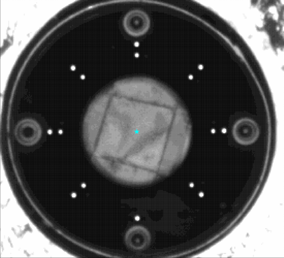
Figure 4 shows an example of an image taken during flight. The camera is equipped with a $100\text{\,}\mathrm{m}\mathrm{m}$ lens and records images with a resolution of $1360\text{\times}1024$ pixels. For transmission and storage, images are cropped to a region of interest around the LED pattern, but the image analysis considers the entire image. The LEDs are mounted to a disk-shaped circuit board painted black and shaded from the sun with the help of a baffle. The image analysis begins by finding this circuit board as an annulus of dark pixels on the bright background. The bright region at the center of the image is the entrance window to the polarimeter, covered in thin aluminum foil and kapton tape. Within the annulus, LEDs are detected as clusters of bright pixels. The known pattern of LEDs is then fitted to the distribution of these clusters by shifting, rotating, and scaling the pattern in order to minimize the distances between LED positions in the pattern and clusters in the image.

Through the entirety of the flight, we found an RMS spread of the focal spot location of $0.63\text{\,}\mathrm{m}\mathrm{m}$ horizontally and $0.28\text{\,}\mathrm{m}\mathrm{m}$ vertically (see Fig. 5). All alignment measurements were $<3\text{\,}\mathrm{m}\mathrm{m}$ from the center of the scattering element, and the focal point was within $1\text{\,}\mathrm{m}\mathrm{m}$ of the center $73\text{\,}\mathrm{\%}$ of the time. We also observe a significant correlation between horizontal alignment offset and pointing elevation, and the horizontal RMS spread during the GX 301-2 and Vela X-1 observations is $0.47\text{\,}\mathrm{m}\mathrm{m}$ and $0.30\text{\,}\mathrm{m}\mathrm{m}$, respectively. The fact that changes in pointing elevation result in a horizontal instead of vertical offset has been observed in pre-flight tests of the truss structure and we attribute it to torsional deformations. Since the truss structure has been cut during the recovery of the polarimeter after the flight, we do not have the ability to verify this hypothesis.

Figure 6 shows the temperature of each of the 12 aluminum joints throughout the flight. After the launch, joint temperatures reflect the decreasing air temperature until the balloon crosses the tropopause. Temperatures start diverging after the balloon reached the floating altitude of $130true000\text{\,}\mathrm{f}\mathrm{t}$ due to the low air density. At this altitude temperature is determined by solar illumination and exposure of each joint to the ground or cold cloud cover. The two joints that hold the latch bar show greater variation because the latch bar was not wrapped in aluminized mylar as safety precaution. Mylar could interfere with the latch, if were to come lose during launch. The latch bar holds the mechanical assembly that arrests the truss in its stowed position during ascent and decent.

During the design phase the anticipated truss configuration was analyzed in Thermal Desktop, RadCAD, and SINDA [20]. Two cases were analyzed: a hot case with an environment representative of the conditions near the December solstice and a cold case representing the conditions at the end of January. Since the entire flight took place close to the solstice, only the hot case is shown in Fig. 6. Disregarding the extremes due to the exposed latch bar, which was not modelled, and data towards the end of the flight when the balloon was at a very low altitude, three main observations can be made: (1) most joint temperatures were higher than predicted; (2) the large spread of temperatures between individual joints of about $20\text{\,}\mathrm{\SIUnitSymbolCelsius}$ between the warmest and coldest joints was not anticipated; (3) the model underestimates the observed diurnal variation. These facts indicate that the performance of the insulating layers on the truss was overestimated in the model. However, despite this, the telescope achieved the required alignment performance.

The Wallops Arc Second Pointer (WASP) was utilized to provide attitude control for the 8-m truss-mounted instrument. The WASP is a balloon-borne fine-pointing system designed to point telescopes and other instruments on balloon gondolas at targets with arc-second accuracy and stability [26]. The WASP system points an instrument using a gondola-mounted pitch/yaw articulated gimbal. The range of motion of the yaw-gimbal is purposely minimized to reduce kinematic coupling during fine pointing. Thus, the gondola itself is suspended beneath a standard NASA Rotator to provide large angle azimuth targeting and coarse azimuth stabilization.

Instrument attitude is computed by integrating incremental angles (delta-Theta) output from an LN251 system. Quaternion solutions from a Camera Attitude and Reference Determination System (CARDS) star tracker are augmented by the integrated attitude solution utilizing a 6-state Extended Kalman Filter. The CARDS was developed as a WASP subsystem to be robust in the face of significant bright-sky background, typical of daytime balloon flight operations.

This flight was the 7^th flight of the WASP system and was the second flight with the X-Calibur payload. However, the Antarctica flight provided a number of firsts for WASP. It was the first multi-day flight of WASP. It was first the time WASP performed an in-flight alignment between the star tracker, inertial measurement unit, and a science instrument. It was the first flight of WASP integrated with the improved rotator electronics system. It was the first attempt at fully autonomous control system operations.

The in-flight alignment of the star tracker with the instrument was achieved by comparing the star tracker image to a forward-looking camera mounted to the central borehole of the X-ray mirror. The alignment between this on-axis camera and the X-ray mirror had been calibrated in the lab.

The primary science requirement levied on the WASP was to hold the X-ray mirror axis to within 30 arc seconds (3$\sigma$) of the source during each observation. 30 arc seconds correspond to 1.16 mm in the focal plane of the telescope. During the flight, WASP maneuvered to and acquired multiple X-ray sources and provided pointing stability between 1.0 and 3.6 arc seconds (3$\sigma$) while on the source.

WASP pointing was spent primarily on two targets: GX 301-2 and Vela X-1. The targets were complementary in that there were no times when both sources violated a lower or upper look elevation constraint. There was always one target available for observation. Pointing at each target followed a “nodding” program where the control system cycled the instrument between time on source and time on background at varying locations relative to the source (pitch up/down, yaw right/left, see Fig. 7). The frequency of this nodding pattern was adjusted to the observed sources. For the pulsars Vela X-1 and GX 301-2, it was chosen such that each on-source observation would be longer than one pulsar period ($\sim 10\text{\,}\mathrm{m}\mathrm{i}\mathrm{n}$ and $\sim 15\text{\,}\mathrm{m}\mathrm{i}\mathrm{n}$, respectively). Frequent off-source observations are necessary to measure the background, which may change with pointing elevation, balloon altitude and time.

Figure 8 (top) shows the pointing error experienced by the control system during the first observation of GX 301-2 as the system cycled on and off of the source. The range of pointing performance experienced during this observation was typical for that of the flight. While on source, the yaw error was generally kept within 1.5 arc seconds. The pitch error performance varied between 1 and 1.5 arc seconds for most of the observation. At the higher elevations experienced toward the end of the observation, pitch error and pitch torques increased (see Fig. 8, bottom). We interpret this as an indication, that the system picked up some mechanical interference between one of the wire cable loops and a gimbal. Even still, pointing stability was maintained well within the experiment requirements.

To verify in the field that the mirror is aligned with the polarimeter, we developed a portable system that attaches to the front of the telescope. It consists of a $14\text{\,}\mathrm{i}\mathrm{n}\mathrm{c}\mathrm{h}$-diameter Celestron off-the-shelf Schmidt-Cassegrain telescope operated as a light collimator rather than collector: at the focal point, we position the end of an optical fiber pigtailed to a Thorlabs $637.4\text{\,}\mathrm{n}\mathrm{m}$ Class 3R laser.

The laser is bright enough that the focal spot can be observed without darkening the room, and the telescope is large enough that when mounted in front of the X-ray mirror it illuminates a significant fraction of the mirror. As the optical telescope does not illuminate the entire X-ray mirror, the image of the light source in the detector plane does not fully correspond to the image of a celestial source, and the position may be offset slightly. The offset will be smaller than the angular resolution of the mirror. We coarsely collimate the light from the telescope by adjusting the telescope focus so that at some large distance the beam is still $\sim 14\text{\,}\mathrm{i}\mathrm{n}\mathrm{c}\mathrm{h}\mathrm{e}\mathrm{s}$ in diameter. Then, after mounting the telescope to the front bulkhead, we finely adjust the focus to optimize the point spread function seen by the forward looking camera. The telescope is mounted on top of tilt and rotation stages to adjust the position of the light source in the forward looking camera to match its position during calibration in the X-ray optics lab at Goddard Space Flight Center. By then comparing the position of the focal spot on the detector in the back-looking camera to its calibration, we can verify that the X-ray mirror is aligned with the detector. Using this technique, we verified that the X-ray mirror was aligned within $0.39\text{\,}\mathrm{m}\mathrm{m}$ of the center of the Be scattering element.

In order to allow projection of measured polarization angles onto the sky, the roll angle of the polarimeter was calibrated with respect to the pointing system’s bank angle as follows. With the truss oriented in a stow position (with a truss elevation at 6^∘), the polarimeter was rotated such that one of the detector segments was oriented approximately vertically. Two angles were measured simultaneously: the offset of the pointing system’s roll angle from the direction to the center of the earth (reading out the LN 251), and the offset of the polarimeter’s side from the direction of to the center of the earth (measured with the help of an engineer’s spirit level and the back looking camera taking images of the detector and the level). These two measurements allowed us to reference the polarimeter’s roll angle relative to the pointing system’s roll angle. During the flight, the pointing system then reports the roll angle offset to the celestial north pole, and the polarimeter reports its roll angle. Together with the ground calibration results, the angle between the celestial north and the detector orientation can be determined. For each detected event, we can thus infer the angle $\chi$ between the scattering direction and the celestial north pole.

The data acquisition CPU is part of the continuously rotating polarimeter assembly. A second CPU mounted on the pointed optical bench communicates with the data acquisition CPU via a custom four-wire protocol with a bitrate of $6.25\text{\,}\mathrm{M}\mathrm{b}\mathrm{i}\mathrm{t}\mathrm{/}\mathrm{s}$ through an 8-pin rotating connector that also carries power and the pulse-per-second signal from the GPS for event time tagging. Finally, a third CPU connected to the truss-mounted CPU via Ethernet is responsible for telemetry to the ground. X-Calibur communicated via several channels provided provided by Columbia Scientific Balloon Facility’s Support Instrumentation Package (SIP), as well as a line-of-sight downlink via a $150\text{\,}\mathrm{k}\mathrm{b}\mathrm{i}\mathrm{t}$ digital L-band transmitter while the payload was within about $300$ miles of the launch site. Over-the-horizon downlink was available via two Tracking and Data Relay Satellite System (TDRSS) antennas with varying bandwidth between $3\text{\,}\mathrm{k}\mathrm{b}\mathrm{i}\mathrm{t}\mathrm{/}\mathrm{s}$ and $83\text{\,}\mathrm{k}\mathrm{b}\mathrm{i}\mathrm{t}\mathrm{/}\mathrm{s}$, respectively, an IP-based Iridium Pilot system²² 2 Allocation for detector operations and polarimeter data downlink. Additional bandwidth on the Iridium Pilot system was used by the WASP pointing system. at $40\text{\,}\mathrm{k}\mathrm{b}\mathrm{i}\mathrm{t}\mathrm{/}\mathrm{s}$, and low-rate housekeeping data via Iridium short-burst data (SBD) and dial-up if needed. Data downlinks were used in a redundant fashion, and all except the line-of-sight transmitter were shared between detector operations and the WASP. Configurable data prioritization and filtering was used to adapt to changing available bandwidth during the flight. Command uplink was provided by a line-of-sight antenna from McMurdo, as well as via Iridium Pilot, short-burst data, and dial-up. A TDRSS uplink was established once a day for higher-rate commanding, in particular with the intent to upload new observation schedules to WASP. After landing, the payload still functioned, solar panels still provided power, and due to the unexpectedly short flight, we were able to download all data directly from the truss-mounted CPU via Iridium Pilot, recovering all data that may have been lost in downlink. All data presented in this paper were obtained in this way. Note, however, that we still suffered some data loss due to the connection between the rotating readout CPU and the truss-mounted CPU as discussed in Section 3.3.

In order to achieve the best possible detector performance, we characterized $83$ ASICs and 19 CZT detectors available at Washington University in St. Louis, from which we assembled the 17 CZT/ASIC assemblies used in X-Calibur. We started by evaluating each ASIC without connecting a CZT detector. Using an oscilloscope connected to the analog output pin of the ASIC and the ASIC’s internal $200\text{\,}\mathrm{f}\mathrm{F}$ test pulse capacitor, we measured the gain of each channel, operating at the nominal setting of $57\text{\,}\mathrm{m}\mathrm{V}\mathrm{/}\mathrm{f}\mathrm{C}$, and the baseline RMS noise voltage. Using the measured gain, we converted the RMS noise into equivalent noise charge (ENC). Typical ENC for a good channel is $<200\text{\,}\mathrm{e}^{-}$, with the best channels reaching $~150\text{\,}\mathrm{e}^{-}$. We also tested the linearity of the front end and recorded a sample of waveforms, which we inspected visually. CZT detector crystals were generally found to be of good quality, and their selection had little impact on detector performance.

Based on these results, we assembled units of CZT detectors with two ASICs each using the ASICs with the lowest noise and largest number of working channels, that did not exhibit any strong nonlinearities or unusual pulse shapes. Each CZT detector is bonded to a ceramic circuit board using a flip-chip process and the circuit board is plugged into the ASIC boards using two 32-pin connectors. These packages are then plugged into the digital front-end boards using another set of connectors on the ASIC board. This modular structure allows replacement of individual ASIC boards and CZT detectors even after assembly. All of these CZT/ASIC assemblies were then tested individually by obtaining spectra with a ${}^{152}\text{Eu}$ source to verify their performance, and in order to test the CZT detectors themselves. Key criteria were the number of working channels, energy threshold, and energy resolution of the assembly. Poorly contacted pixels can lead to additional inoperable channels, and leakage currents can result in increased noise, which often required deactivation of additional channels. A small number of CZTs were found to suffer from these problems and were replaced. Thus, we systematically assembled the 17 best-performing packages, which we subsequently used when assembling the four front-end boards.

The X-Calibur CZT detectors were calibrated at Washington University in St. Louis using an $0.2\text{\,}\text{$\mu$}\mathrm{C}\mathrm{i}$ ${}^{152}\text{Eu}$ calibration source. The isotope with a half life of about 13 years emits several gamma-ray lines in the energy range of interest: a line complex consisting of the ${}^{152}\text{Sm}_{\text{K\textalpha}}$ and ${}^{152}\text{Sm}_{\text{K\textbeta}}$ X-ray lines around $40\text{\,}\mathrm{k}\mathrm{e}\mathrm{V}45\text{\,}\mathrm{k}\mathrm{e}\mathrm{V}$ and a γ-ray line at $121.782\text{\,}\mathrm{k}\mathrm{e}\mathrm{V}$ [29]. The count rate due to the source exceeded background rates by about three orders of magnitude.

The $3946\text{\,}\mathrm{k}\mathrm{e}\mathrm{V}$ line complex and the $121\text{\,}\mathrm{k}\mathrm{e}\mathrm{V}$ line were jointly fit by the following two functions:

where the line energies $E_{i}$ and relative strengths $a_{i}$ in (1) are given in Table 2, $E_{121}=$121.7817\text{\,}\mathrm{k}\mathrm{e}\mathrm{V}$$, the energy is related to ADC counts using the linear relation $E=(\mathrm{ADC}-b)/m$, and $b$, $m$, $C_{40}$, $A_{40}$, $\sigma_{40}$, $y_{40}$, $C_{121}$, $A_{121}$, $\sigma_{121}$, and $y_{121}$ are fit parameters. In both functions, the onset of the Compton continuum due to scattering in the detector is approximated by the smooth ramp function with scales $y_{40}$ and $y_{121}$. Each fit is performed twice, and during the second iteration, the fit ranges are set to $E_{2}-4\sigma_{40}$ to $E_{4}+4\sigma_{40}$ for $f_{40}$ and to $E_{121}\pm 4\sigma_{121}$ for $f_{121}$, where $\sigma_{40}$ and $\sigma_{121}$ are obtained from the first iteration. An example fit is shown in Fig. 12. Typical values are $b\approx$415\text{\,}\mathrm{A}\mathrm{D}\mathrm{C}$$ and $m\approx$2.9\text{\,}\mathrm{A}\mathrm{D}\mathrm{C}\mathrm{/}\mathrm{k}\mathrm{e}\mathrm{V}$$. Figure 11 shows the distribution of energy resolutions at $\sim 40\text{\,}\mathrm{k}\mathrm{e}\mathrm{V}$ and $121\text{\,}\mathrm{k}\mathrm{e}\mathrm{V}$ of all active channels. We find a median FWHM resolution of $3.35\text{\,}\mathrm{k}\mathrm{e}\mathrm{V}$ and $3.60\text{\,}\mathrm{k}\mathrm{e}\mathrm{V}$, respectively.

Excessively noisy and non-operational channels were deactivated. During the flight $949$ of the 1088 channels ($87\text{\,}\mathrm{\%}$) were working. This number fell slightly short of the target of $90\text{\,}\mathrm{\%}$ working channels, and was accepted in order to achieve a stable detector operation. Using the calibration data, we also determined the energy threshold of each channel. Due to the hysteresis of the threshold discriminator in the ASIC, there is no sharp threshold. Hence, we empirically defined the threshold as the $0.25$^th percentile of all events. The distribution of energy thresholds is shown in Fig. 13.

Figure 14 shows the time difference between consecutive events in X-Calibur throughout the entire flight. From an exponential fit we find a rate of $333\text{\,}\mathrm{H}\mathrm{z}$ for all triggers, and $39\text{\,}\mathrm{H}\mathrm{z}$ for events not vetoed by the anti-coincidence shield.

As described in Section 2.2, the readout dead time for a single-pixel event is $43.6\text{\,}\mathrm{\SIUnitSymbolMicro s}$. From the multiplicity distribution shown in Fig. 15, we estimate an average dead time of $52\text{\,}\mathrm{\SIUnitSymbolMicro s}$. During this dead time, no events will be recorded. Given the trigger rate at float, this corresponds to $1.8\text{\,}\mathrm{\%}$ of events. However, due to the inability of the firmware to distinguish between multiple ASICs read as part of the same trigger or of consecutive triggers, we decided to discard all events with a time difference less than $55\text{\,}\mathrm{\SIUnitSymbolMicro s}$, resulting in an artificial dead time of $1.9\text{\,}\mathrm{\%}$. This artificial dead time can be seen in the inset of Fig. 14 and does not add to the detector readout dead time. The spike at $65\text{\,}\mathrm{\SIUnitSymbolMicro s}$ is currently not fully understood, but likely due to the way subsequent events are time-tagged after being transmitted from the front-end readout to the CPU.

The broad bump at $$0.05\text{\,}\mathrm{s}$<\Delta T<$0.15\text{\,}\mathrm{s}$$ in the distribution of all events in Fig. 14 is due to individual lost data packets. These packets have been lost during transmission through the rotating connector. We are implementing improvements to this link to prevent such data loss during the follow-up mission XL-Calibur.

The anti-coincidence shield performance was tested after the flight with a ${}^{137}\text{Cs}$ radioactive source, which emits $662\text{\,}\mathrm{k}\mathrm{e}\mathrm{V}$ gamma-rays. Since the flight readout board does not have a pulse-height digitization capability, we used an external pre-amplifier (CANBERRA 2005), shaping amplifier (ORTEC 485) and multi-channel analyzer (Amptek 8500D) for the spectral and gain studies. During the flight, we set the PMT high-voltage to $750\text{\,}\mathrm{V}$ for all PMTs and the veto threshold to $30$ and $300$ channels for the PMTs connected to the top and bottom part of the shield, respectively. For the bottom part, we were able to set the threshold as low as $30$ channel, but increased to $300$ due to the high rate of cosmic-rays during the flight, which would have resulted in an unacceptably large dead time.

With the flight operation high-voltage of $750\text{\,}\mathrm{V}$, we obtained ${}^{137}\text{Cs}$ spectra for each PMT and confirmed that the gain is consistent within a factor of $\sim 1.5$ within each shield part. In order to measure the trigger threshold, the signal from one PMT is input to the external spectral measurement, and a trigger signal is generated from the other three PMTs using the flight electronics. The spectra of both top and bottom parts are obtained with (red) and without (blue) the trigger from the flight board and shown in Fig. 16. For the bottom, the flight board spectrum shows a cut-off around $1200$ channel which corresponds to $\sim 1.4\text{\,}\mathrm{M}\mathrm{e}\mathrm{V}$. Since the veto comparator checks the signal after summing all 4 PMTs (we use only 3 PMT signals for the trigger in this measurement), we estimate the flight veto threshold for the 2018/19 flight at $$1.4\text{\,}\mathrm{M}\mathrm{e}\mathrm{V}$/(4/3)\sim$1.1\text{\,}\mathrm{M}\mathrm{e}\mathrm{V}$$. In case of the top part, the cut-off appears at $\sim 400$ channel corresponding to $\sim 200\text{\,}\mathrm{k}\mathrm{e}\mathrm{V}$, an estimated flight veto threshold of $\sim 150\text{\,}\mathrm{k}\mathrm{e}\mathrm{V}$. The high threshold of the bottom shield was necessary in order to keep the dead time below $5\text{\,}\mathrm{\%}$ (see Section 4 and Fig. 24).

These measurements show that it will be possible to significantly reduce the threshold of the bottom part of the CsI shield. The $6.4\text{\,}\mathrm{\SIUnitSymbolMicro s}$ duration of the veto signal was necessitated by the time constant of the amplifier. For future flights of XL-Calibur, we will modify the analog circuit of the readout board to reduce the time constant of the amplifier. Furthermore, we will tune the duration and timing of the digital anti-coincidence flag in order to reduce the dead time and maximize veto efficiency. Finally, the XL-Calibur shield will be made of BGO, which enables a more compact geometry due to its higher stopping power and inherently provides faster scintillation signals [30].

References

- [1] H. Krawczynski, A. Garson, Q. Guo et al., Scientific prospects for hard X-ray polarimetry, Astropart. Phys. 34 (2011) 550–567. arXiv:1012.0321.
- [2] M. C. Weisskopf, E. H. Silver, H. L. Kestenbaum, K. S. Long, R. Novick, A precision measurement of the X-ray polarization of the Crab Nebula without pulsar contamination., Astrophys. J. Lett. 220 (1978) L117–L121. doi:10.1086/182648.
- [3] M. Chauvin, H. G. Florén, M. Friis et al., Shedding new light on the Crab with polarized X-rays, Sci. Rep. 7 (2017) 7816. arXiv:1706.09203.
- [4] H.-C. Li, N. Produit, S.-N. Zhang et al., Gamma-Ray Polarimetry of the Crab Pulsar Observed by POLAR, arXiv e-prints (2022) arXiv:2202.10877arXiv:2202.10877.
- [5] F. Aharonian, H. Akamatsu, F. Akimoto et al., Detection of polarized gamma-ray emission from the Crab nebula with the Hitomi Soft Gamma-ray Detector, Pub. Astron. Soc. Japan 70 (2018) 113. arXiv:1810.00704.
- [6] H. Feng, H. Li, X. Long et al., Re-detection and a possible time variation of soft X-ray polarization from the Crab, Nature Astron. 4 (2020) 511–516. arXiv:2011.05487.
- [7] S. V. Vadawale, T. Chattopadhyay, N. P. S. Mithun et al., Phase-resolved X-ray polarimetry of the Crab pulsar with the AstroSat CZT Imager, Nature Astronomy 2 (2018) 50–55. doi:10.1038/s41550-017-0293-z.
- [8] M. Forot, P. Laurent, I. A. Grenier, C. Gouiffès, F. Lebrun, Polarization of the Crab Pulsar and Nebula as Observed by the INTEGRAL/IBIS Telescope, Astrophys. J. Lett. 688 (2008) L29. arXiv:0809.1292.
- [9] A. J. Dean, D. J. Clark, J. B. Stephen et al., Polarized Gamma-Ray Emission from the Crab, Science 321 (2008) 1183. doi:10.1126/science.1149056.
- [10] M. Chauvin, J. P. Roques, D. J. Clark, E. Jourdain, Polarimetry in the Hard X-Ray Domain with INTEGRAL SPI, Astrophys. J. 769 (2013) 137. arXiv:1305.0802.
- [11] E. Jourdain, J. P. Roques, 2003-2018 Monitoring of the Crab Nebula Polarization in Hard X-Rays with INTEGRAL SPI, Astrophys. J. 882 (2019) 129. arXiv:1907.09341.
- [12] M. C. Weisskopf, E. H. Silver, H. L. Kestenbaum et al., Search for X-ray polarization in Cygnus X-1., Astrophys. J. Lett. 215 (1977) L65–L68. doi:10.1086/182479.
- [13] M. C. Weisskopf, H. L. Kestenbaum, K. S. Long, R. Novick, E. H. Silver, An upper limit to the linear X-ray polarization of Scorpius X-1., Astrophys. J. Lett. 221 (1978) L13–L16. doi:10.1086/182655.
- [14] K. S. Long, G. A. Chanan, W. H. M. Ku, R. Novick, The linear X-ray polarization of Scorpius X-1., Astrophys. J. Lett. 232 (1979) L107–L110. doi:10.1086/183045.
- [15] K. S. Long, G. A. Chanan, R. Novick, The X-ray polarization of the CYG sources., Astrophys. J. 238 (1980) 710–716. doi:10.1086/158027.
- [16] M. Chauvin, H. G. Florén, M. Friis et al., Accretion geometry of the black-hole binary Cygnus X-1 from X-ray polarimetry, Nature Astronomy 2 (2018) 652–655. arXiv:1812.09907.
- [17] Q. Guo, M. Beilicke, A. Garson et al., Optimization of the design of the hard X-ray polarimeter X-Calibur, Astropart. Phys. 41 (2013) 63–72. arXiv:1212.4509.
- [18] F. Kislat, Q. Abarr, B. Beheshtipour et al., Optimization of the design of X-Calibur for a long-duration balloon flight and results from a one-day test flight, J. Astron. Telesc. Instrum. Syst. 4 (2018) 011004. doi:10.1117/1.JATIS.4.1.011004.
- [19] M. Beilicke, F. Kislat, A. Zajczyk et al., Design and Performance of the X-ray Polarimeter X-Calibur, J. Astron. Instrum. 3 (2014) 1440008. arXiv:1412.6457.
- [20] F. Kislat, B. Beheshtipour, P. Dowkontt et al., Design of the Telescope Truss and Gondola for the Balloon-Borne X-ray Polarimeter X-Calibur, J. Astron. Instrum. 6 (2017) 1740003. arXiv:1701.04536.
- [21] Q. Abarr, M. Baring, B. Beheshtipour et al., Observations of a GX 301-2 Apastron Flare with the X-Calibur Hard X-Ray Polarimeter Supported by NICER, the Swift XRT and BAT, and Fermi GBM, Astrophys. J. 891 (2020) 70. arXiv:2001.03581.
- [22] J. Tueller, H. A. Krimm, T. Okajima et al., InFOCS Hard X-ray Imaging Telescope, Exp. Astron. 20 (2005) 121–129. doi:10.1007/s10686-006-9028-3.
- [23] T. Okajima, K. Tamura, Y. Ogasaka et al., Characterization of the supermirror hard-x-ray telescope for the InFOCS balloon experiment, Appl. Optics 41 (2002) 5417–5426. doi:10.1364/AO.41.005417.
- [24] F. Berendse, S. M. Owens, P. J. Serlemitsos et al., Production and Performance of the InFOCS 20-40-keV Graded Multilayer Mirror, Appl. Optics 42 (2003) 1856–1866. doi:10.1364/AO.42.001856.
- [25] Y. Ogasaka, K. Tamura, R. Shibata et al., Characterization of a Hard X-ray Telescope at Synchrotron Facility SPring-8, Jpn. J. Appl. Phys. 47 (2008) 5743. doi:10.1143/JJAP.47.5743.
- [26] D. W. Stuchlik, The Wallops Arc Second Pointer – A Balloon Borne Fine Pointing System, in: AIAA Balloon Systems Conference, Proc. AIAA AVIATION Forum, 2015. doi:10.2514/6.2015-3039.
- [27] E. A. Wulf, B. F. Phlips, W. Neil Johnson et al., Compton imager for detection of special nuclear material, Nucl. Instrum. Meth. Phys. Res. A 579 (2007) 371–374. doi:10.1016/j.nima.2007.04.085.
- [28] G. de Geronimo, J. Fried, E. Frost et al., Front-End ASIC for a Silicon Compton Telescope, IEEE Trans. Nucl. Sci. 55 (2008) 2323–2328. doi:10.1109/TNS.2008.2001410.
- [29] M.-M. Bé, V. Chisté, C. Dulieu et al., Table of Radionuclides, Vol. 2 of Monographie BIPM-5, Bureau International des Poids et Mesures, Pavillon de Breteuil, F-92310 Sèvres, France, 2004. URL http://www.bipm.org/utils/common/pdf/monographieRI/Monographie_BIPM-5_Tables_Vol2.pdf
- [30] Q. Abarr, H. Awaki, M. G. Baring et al., XL-Calibur - a second-generation balloon-borne hard X-ray polarimetry mission, Astropart. Phys. 126 (2021) 102529. arXiv:2010.10608.
- [31] S. Agostinelli, J. Allison, K. Amako et al., GEANT4—a simulation toolkit, Nucl. Instrum. Meth. Phys. Res. A 506 (2003) 250–303. doi:10.1016/S0168-9002(03)01368-8.
- [32] J. Allison, K. Amako, J. Apostolakis et al., Geant4 developments and applications, IEEE Trans. Nucl. Sci. 53 (2006) 270–278. doi:10.1109/TNS.2006.869826.
- [33] J. Allison, K. Amako, J. Apostolakis et al., Recent developments in GEANT4, Nucl. Instrum. Meth. Phys. Res. A 835 (2016) 186–225. doi:10.1016/j.nima.2016.06.125.
- [34] F. Lei, A. Hands, S. Clucas, C. Dyer, P. Truscott, Improvement to and Validations of the QinetiQ Atmospheric Radiation Model (QARM), IEEE Transactions on Nuclear Science 53 (2006) 1851–1858. doi:10.1109/TNS.2006.880567.
- [35] F. Kislat, M. Beilicke, Q. Guo, A. Zajczyk, H. Krawczynski, An unfolding method for X-ray spectro-polarimetry, Astropart. Phys. 64 (2015) 40–48. arXiv:1411.5037.
- [36] M. C. Weisskopf, B. Ramsey, S. O’Dell et al., The Imaging X-ray Polarimetry Explorer (IXPE), in: Proc. SPIE, Vol. 9905 of Society of Photo-Optical Instrumentation Engineers (SPIE) Conference Series, 2016, p. 990517. doi:10.1117/12.2235240.
- [37] M. C. Weisskopf, B. Ramsey, S. L. O’Dell et al., The Imaging X-ray Polarimetry Explorer (IXPE), Res. Phys. 6 (2016) 1179–1180. doi:10.1016/j.rinp.2016.10.021.
- [38] M. Weisskopf, An Overview of X-Ray Polarimetry of Astronomical Sources, Galaxies 6 (2018) 33. doi:10.3390/galaxies6010033.
- [39] H. S. Krawczynski, D. Stern, F. A. Harrison et al., X-ray polarimetry with the Polarization Spectroscopic Telescope Array (PolSTAR), Astropart. Phys. 75 (2016) 8–28. arXiv:1510.08358.
- [40] H. L. Marshall, H. M. Günther, R. K. Heilmann et al., Design of a broadband soft x-ray polarimeter, J. Astron. Telescopes Instrum. Syst. 4 (2018) 011005. doi:10.1117/1.JATIS.4.1.011005.
- [41] W. B. Iwakiri, J. K. Black, R. Cole et al., Performance of the PRAXyS X-ray polarimeter, Nucl. Instrum. Meth. Phys. Res. A 838 (2016) 89–95. arXiv:1610.06677.
- [42] H. Krawczynski, G. Matt, A. R. Ingram et al., Using X-Ray Polarimetry to Probe the Physics of Black Holes and Neutron Stars, Bulletin of the American Astronomical Society 51 (2019) 150. arXiv:1904.09313.
- [43] K. Jahoda, H. Krawczynski, F. Kislat, H. Marshall, T. Okajima, The X-ray Polarization Probe mission concept, Bulletin of the American Astronomical Society 51 (2019) 181. arXiv:1907.10190.