A framework for topological music analysis (TMA)
Abstract
In the present article we describe and discuss a framework for applying different topological data analysis (TDA) techniques to a music fragment given as a score in traditional Western notation. We first consider different sets of points in Euclidean spaces of different dimensions that correspond to musical events in the score, and obtain their persistent homology features. Then we introduce two families of simplicial complexes that can be associated with chord sequences, and leverage homology to compute their salient features. Finally, we show the results of applying the described methods to the analysis and stylistic comparison of fragments from three Brandenburg Concertos by J.S. Bach and two Graffiti by Mexican composer Armando Luna.
keywords
topological data analysis (TDA); simplicial complexes; persistent homology; music analysis2020 Mathematics Subject Classification: 00A65; 55N31
Introduction.
In this work we present several ways of treating data extracted from a digital music score, and discuss the results of applying some tools and techniques from algebraic topology (mainly simplicial homology) to music analysis. Our motivation is to incorporate new scopes and computational tools to music analysis, hoping they will contribute in establishing a theoretical and practical framework suitable for analyzing music in a wide variety of languages and styles (ideally, in any language or style).
Usually, music is analyzed through the lens of a very specific framework, such as the traditional Western tonal theory, the jazz modal harmonic setting, the dodecaphonic technique, the classical Indian music tradition, etc. Of course all of these provide valuable and useful analytical techniques and terms to deal with the elements and processes which occur in their respective musical systems. Nevertheless, when trying to describe, within a single framework, musical objects and phenomena found in a diversity of repertoire or musical cultures, musicians and musicologists often find less complete and consistent methodological resources. Thus, for certain analytical and musicological purposes, it is desirable to work in a more general framework within which to speak about many types and styles of music, in equal terms, though this might necessarily lead to losing some of the fine details given by more particular analytical scopes.
In recent years, there has been a wide range of works pointing in this direction, especially coming from applied mathematics, introducing general theoretical and methodological frameworks that include the use ofconcepts and tools from very different mathematical areas (see, for example: Beran and Mazzola 1999; Mazzola 2012; Tymoczko 2010; Andreatta 2003; Szeto and Wong 2006; Agustín-Aquino et al. 2009; Pareyón 2011; Estrada 2011; Bergomi 2015; Padilla et al. 2017 ). In search of contributing to this task, we focus on some mathematical models and tools that seem pertinent to describe data codified (or codable) in musical scores (computationally we will constrain ourselves to working with fragments written in traditional Western music notation, though this does not restrict us to Western music tradition or repertoire exclusively). Of particular interest to us is the idea of applying techniques of data analysis to musical information, and for the present article we work with techniques from topological data analysis (TDA). The application of algebraic topology concepts and techniques to describe harmonic structure in music has been treated in several works, for example: Bigo, Giavitto, and Spicher 2011; Sethares and Budney 2014; Bigo et al. 2013; Bigo and Andreatta 2016; Giavitto and Spicher 2016; Bergomi 2015; Bigo and Andreatta 2019; Bergomi and Baratè 2020; Sassone et al. 2022; Jen-Yu, Shyh-Kang, and Yi-Hsuan 2016.
Through the application of these techniques, we seek to deal directly with the events noted in a score, without assuming any given system of relations between pitches or pitch class sets. In contrast with the classical harmonic or Schenkerian analysis, there is no assumption of a particular or pre-established hierarchical harmonic nor formal system. Also, we may state that our scope differs from other methodologies which include some “geometrization” of musical data, such as the Tonnetz and its generalizations. Unlike these models, we do not assume any fixed structure of chords, and do not deal with voice-leading or chord-generation processes. We do not properly deal with chords as defined in traditional music theory. Instead, we part from vertical events, that is, sets of pitches sounding simultaneously (as encoded in the score), which may actually incorporate two or more chords overlapping (as seen under a particular analytical framework). These vertical events are determined by the appearance, disappearance or prolongation of notes in the score.
On one hand, we study the persistent homology (for a presentation on the subject, the reader may refer to the Appendix of this paper) of different sets of points formed from pitch and time data in a score. We consider vertical events both with and without their rhythm and onset in the score. Next, we propose and explore two different ways of constructing sequences of simplicial complexes from chord sequences. One of these constructions coincides with similar scopes in the way of looking at a chord as a simplex on vertices corresponding to pitches or pitch classes (see, for example, Bigo et al. 2013), modeling chords consisting of pitch classes as simplices on vertices. Yet a novelty introduced in this article is another way to construct a simplicial complex that encodes not only pitch but also interval information. Simplicial complexes associated with sequences of chords have been treated in previous works, such as Bergomi 2015; Bergomi and Baratè 2020. We plot as barcodes and persistence diagrams (see the Appendix) the homological features of all such simplicial complexes associated to fragments of different scores, and compare the results, using the bottleneck distance (see the Appendix). Finally, we summarize our results in several dendrograms, and present our conclusions.
For the sake of space, we assume the reader is familiar with the basic post-tonal theory concepts (pitch and interval classes; normal form or order, and interval vector of a chord; see, for example Straus 2016). We present the basics of simplicial and persistent homology at the end of the paper, in the Appendix. For a deeper treatment of homology (homology groups, Betti numbers, Euler characteristic) the reader can refer to, for example, the classic books of Hatcher 2002; Rotman 2013. Persistent homology concepts and methods (Vietoris-Rips complexes, barcodes and persistence diagrams, bottleneck distance) may be consulted in the survey by Edelsbrunner, Harer et al. 2008.
1 Definitions and methods.
We consider music scores written in traditional Western notation. We define vertical events in a music score as tuples containing information of synchronous sounds, usually pitches or pitch classes, possibly together with some other features, such as its onset, duration (rhythm), dynamics (loudness) or timbre (instrumentation). In this work we focus on events given as tuples of pitch classes, with or without their duration and onset.
A vertical event given only by pitch information will be called a chord, and a chord formed by different pitch classes will be referred to as an chord. A music fragment is a (usually assumed finite) sequence (ordered set) of vertical events. Given a fragment , the interval of events is the sequence .
This segmentation of events in the score does not take into account any other information other than their sequential order. In the case of “continuous” (smooth) music passages or textures, one could identify starting points without the need of counting beats, and smooth fade-in/fade-out elements by a gradual discrete approximation. In any case, a digital measurable score is not absolutely necessary to apply the present model (though it actually could be produced). One may directly define the sequence of events
Working on sequences of events indexed by their order of occurrence allows us to easily focus merely in harmonic changes, and, when necessary, take into account time information (duration and onset, encoded as separate coordinates of an event). This implies that there may be chords appearing more than once in , when they occur at different times (except in cases such as the example below, when a distinguished coordinate such as the onset is included). We will always take into account the index of a chord or event in the sequence being considered. Thus, technically we should write . However, when there may be no confusion we will write only as to lighten notation. This notation also attempts to show the possible time-dependence of the consecutive occurrence of two or more chords, and helps us grasp harmonic progressions independently of the rhythmic values involved. Simplices corresponding to repeated chords will only appear once in the complex of cumulative events. Also, in the embedding of chords (without rhythm/onset) in , repeated chords are mapped to the same point in
Given a music fragment , we define as the sequence (ordered set) whose term is the chord corresponding to the th vertical event of , . Chords in the set may be expressed in different ways: by their common name (C Major, d minor, F\musSharp diminished, etc.), as a tuple of pitch classes (for example, in ascending order, or following the normal form of the chord), or as a tuple of intervals or interval classes (for example each chord may be expressed as a sequence of intervals starting at the lowest pitch (as in figured bass notation), or as an interval vector as defined in classic post-tonal theory).
For now we restrict ourselves to the setting of pitches within the twelve tone equal temperament and more specifically, their corresponding pitch classes represented as elements of the set of integers modulo , . This assumption allows us to show how these techniques can work in a fairly standard setting. Yet, the same methods can be applied in any other tempered, non-tempered or microtonal setting, making the proper straightforward adjustments to definitions dependant on the number of pitches or pitch classes considered (for example, the mappings defined in 1.2). We may think of our particular setting as a projection of the one considering all cents in one octave. It is also worth mentioning that the possibility of dealing with microvalues of pitch and duration implies that the methodology described may be useful to analyze continuous music, including electronic music, as we could analyze discrete, measurable transcriptions of continuous musical textures.
We point out that the current algorithm used to parse digital scores does not capture certain musical notations, such as grace notes, slurs (prolongation and phrasing), glissandi (unless explicitly written), tempo, metre, measure, and in general all text indications such as dynamics, playing mode, expressive marks, etc.
In order to conduct our harmonic analysis, we remove from the analyzed scores all staves containing unpitched percussion instruments11 1 In general, notes representing unpitched sounds could be included in the analysis, for instance assigning a numerical “pitch” value sufficiently distant from the ones representing actual pitches.. Time durations and positions will be expressed (with decimal values) in quarter notes (e.g., one eight rhythm , etc.). We point out this does not imply restricting ourselves to notes with onsets on integer quarter beats. The quarter note value is only taken as time unit; we could well establish the use of miliseconds, for instance. It is pertinent to point out that the specific measure units chosen either for time or pitch will determine the point clouds and simplicial complexes associated to musical events. Nevertheless, homeomorphic data encodings (change of units) lead to similar shape features under TDA analyses, being homology a topological invariant.
Let us exemplify these definitions:
Example 1.1.
Let us consider the first two measures (see figure 1) of Mexican composer Armando Luna22 2 Armando Luna Ponce (1964-2015). Mexican composer born in the city of Chihuahua. He studied at the National Conservatory of Music of Mexico (where he later taught composition and music analysis) and the Carnegie Mellon University in the U.S.A.. He mainly produced chamber and symphonic music for acoustic instruments, in what he came to name a ludic-eclectic-neorampageous style. Many of his pieces take the suite structure of brief movements as a model, incorporating Renaissance and Baroque dances from the European traidition as well as many other genres from both academic and folk origins. Also, a considerable amount of his works are hommages dedicated to different composers of the Western academic music pantheon, whose language and style are synthesized and reinterpreted.’s Graffiti Hommage to Franz Joseph Haydn (G.H. to F.J.H.), belonging to his Graffiti, a series of miniatures written for ensemble in 2006 as musical hommages dedicated to different composers. Each Graffiti is built upon the motif corresponding to the musical translation of the name of the composer to whom it is dedicated, according to the following letter equivalences:
A=la, B=si\musFlat, C=do, D=re, E=mi, F=fa, G=sol, H=si, S=mi\musFlat. 33 3 The equivalences of letters A,B,…,H correspond to the usual German letter system for the notes of the diatonic scale. The equivalence S=mi\musFlat also comes from the German ’Es’, which stands for E\musFlat and is pronounced like the letter ’s’. It was used for example by Shostakovich to musically encode his name as the motif re-mi-do-si (D-S-C-H). See, for example DSCH motif in Wikipedia.
These pieces incorporate some of the most characteristic elements
in the styles of composers Johann Sebastian Bach, Franz Joseph Haydn,
Bela Bartók, Dave Brubeck, and seven others, as seen and condensed
by Luna through his own language. You may listen to the recording
of Graffiti by the Present Music ensemble here.

Below we present the sequence of the events of the music fragment corresponding to the first two measures of Luna’s G.H. to F.J.H, given as triads of the form
That is, from score in figure 1 we get the following music fragment:
Of course we may get several music fragments for the same score, as events may be described in several different ways, for example as chords only, or adding some other relevant information found in the digital score. Observe that an event is generated every time there is a change in the notes sounding simultaneously according to the score. Vertical events are taken as notes with the same rhythmic value. Articulation (namely staccato) does not affect the duration of notes. If pitches last longer than the vertical event’s associated rhythmic value, some pitch classes will appear in the subsequent events in order to fill their actual duration according to the score. Note for example that events and , respectively starting at time positions and , show the fact that chord , where pitch class has rhythmic value (a sixteenth note) in the score while the others last for quarters, is followed by , with a rhythmic value of . Besides that, grace notes are considered as part of the chord they precede. We point out that the chord is the only repeated chord in this sequence, and it appears twice: at the and then at the positions. Periodic decimal temporal values have been truncated.
Now from the above fragment , we get
Throughout the rest of the text, we will be ommiting subindices of chords and events.
In this work we deal with given events from different perspectives, encoding them in different ways, for example
Throughout this paper, we consider that events are given as tuples of the form
or simply as vectors representing chords (without duration and onset). To deal with tuples constructed through a particular encoding of events, all those representing chords must belong to the same . In this article we describe several ways of encoding chords as tuples in different Euclidean spaces.
1.1 General strategy.
Given a music score, we extract its vertical events as tuples containing the pitch classes in normal form, together with the duration and onset in the score (both in quarter notes) of each event. We also consider similar tuples in which chords are encoded as interval vectors (as defined in post-tonal theory). We point out that any of these representations of chords are a useful abstract standard for dealing with harmony in general (that is, outside the tonal context), but imply some loss of information, such as voicings and inversions of chords, as well as voice leading. To take into account such aspects, we need to consider some particular representation that encoded them, for instance modeling chord connections rather than chords themselves. This leads to other embeddings and associated spaces, such as the connection simplicial complex mentioned in the Conclusions and future work. section. All such events will be analyzed both with and without time values (duration and onset); that is to say, we will be analyzing chords with and without their rhythm and position in time.
One part of our analysis proposal involves classic TDA: musical events are encoded as points in some Euclidean space by means of different embeddings (which we describe in the next subsection), to later calculate their persistent homology under the Euclidean metric (using the Vietoris-Rips filtration; see Appendix). On the other hand, we compute the homology of simplicial complexes directly associated with event intervals, without considering a metric among data points. We exhibit some cases in which these simplicial complexes actually form a filtration (though not associated with a metric).
All computations presented here were done in Python. To parse and extract data from digital symbolic music files we use the Music21 library. For constructing simplicial complexes, obtaining their homologies and generating their barcodes, persistence diagrams and the bottleneck distance between them, we use algorithms from MoguTDA, Ripser and Persim (the latter two are incorporated as modules of the Scikit-TDA library). Also we made use of some standard libraries for Mathematics and plotting, namely NumPy, SciPy and Matplotlib. The scripts used for computations in this paper may be consulted in this github project.
We work with digital symbolic music files corresponding to musical scores. The filetypes acceptable are those supported by Music21 and include MIDI, .XML and .MXL files (Music21 supports many other formats). These digital scores are parsed in Python, after which different lists of meaningful musical data are generated for a given fragment. Each of these lists defines a musical data mapping. In our case, we obtain lists of vertical events given as tuples consisting of the normal form or interval vector of their corresponding chords, posssibly including their duration (given in quarter notes) and offset (position in time from the beginning of the score, also given in quarter notes). These lists are the raw data analyzed by the persistent homology algorithms. We generate and plot the corresponding persistence diagrams for different mappings of data. As we said before, besides calculating the persistent homology of the Vietoris-Rips filtration constructed from a point cloud in some , we also compute and plot the homological features of two families of simplicial complexes associated with chord sequences in the score.
1.2 Persistent homology on various musical data mappings.
In this section we describe several sets of data points (in different Euclidean spaces) associated with a given music fragment . Concretely, we distinguish six different ways of generating tuples in Euclidean spaces of different dimensions, from vertical events in . We refer to these sets of tuples as data mappings (as not to confuse them with data sets, which usually would mean the possible sets of scores or fragments analyzed), and number them from I through VI. The first two mappings we consider (I and II) consist of points that stand for vertical events in a fragment and incorporate temporal data: each event is translated as a tuple of pitch or interval classes, together with a rhythmic (duration) value and a onset in time, both measured in quarter notes (see example 1.1). The rest of the mappings (III, IV, V, and VI) contain only pitch and/or interval information from each event, that is, they focus only on harmonic aspects of . After generating the data points of each mapping, we run upon each a persistent homology analysis, and plot the resulting persitence diagrams or barcodes. Then we compare persistence diagrams coming from different scores in each mapping by using the bottleneck distance, which is a standard tool for such task. Thus, we are able to depict in dendrograms these distances among corresponding data mappings from such examples. This lets us establish a certain notion of closeness between pieces and styles. It is important to note that the persistent homology of all mappings except I and V remains invariant under transposition of the score by any interval; that is, the bottleneck distance between persistence diagrams of a fragment and its transpositions is in all other mappings (II, III, IV and VI). So data mappings I and V are the ones actually measuring the “tonality”, “tonic” or current transposition of the score in question.
To illustrate the persistence diagrams obtained for each mapping, we take the same fragment treated in example 1.1, corresponding to the two measures shown in figure 1. Colors in persistence diagrams correspond to different dimensions (computed here up to dimension , due to computational time 44 4 For some tests including higher dimensions in homology, ran over -bar samples ( event-points), there were overflow problems in the execution of the script. As said in the documentation of the Ripser library: “[In] It [sic] practice, anything above is very slow.”). For barcode plots we use two different colors: teal for data mappings which include time information (mappings I and II), and dark purple for the rest of mappings.
- •
Data mapping I: We begin considering a set of points or vectors in whose first twelve coordinates correspond to pitch classes, followed by a rhythmic and an onset values expressed in quarter notes. In these vectors, coordinates representing pitch classes of a chord are represented by the integers , according to their ordering in the chord’s normal form. We choose these representatives for each pitch class so we are able to embed any -chord, with . The remaining two coordinates (rhythm and onset) are given as a decimal value representing length and onset in quarter notes. For example, the first three events of the score in figure 1 yield the following associated tuples in :
Applying this mapping to the -event fragment in figure 1 (mm. 1-2 from Luna’s Graffiti Hommage to F.J.H.), we obtain the persistence and barcode diagrams shown in figure 2.


Figure 2: Persistence and barcode diagrams from data mapping I for mm. 1–2 of Luna’s Graffiti Hommage to F.J.H.. Picturing events as pitch-rhythm-onset vectors, this mapping lets us get a notion of their general distribution over time, as well as identify the presence of distinguished harmonic regions. This way, together with an overview of the score, we can have a general impression of the harmonic-rhythmic texture of the fragment in question.
- •
Data mapping II: Similarly, we consider each event as a point in whose first six coordinates are the integers forming the interval vector of its corresponding chord, followed by its duration and onset in time. This mapping reflects similarity in the chord structures present in each event, together with their distribution in time and rhythm. In this case, for the same three events as above, we get:
The resulting diagrams for example 1.1 are shown in figure 3.


Figure 3: Persistence and barcode diagrams from data mapping II for mm. 1–2 of Luna’s Graffiti Hommage to F.J.H.. This data mapping, together with mapping III focus on the types of chords or different chord structures present in the fragment analyzed, as they deal with interval vectors rather than the chords themselves.
Parallel to the above, we also work on sets obtained only from pitch data. That is, we focus especially on harmony, by considering data points containing only pitches in vertical events, forgetting about their distribution along a timeline, their duration, etc. The points generated for this analysis consist of tuples of pitch classes or interval classes. We propose several ways of analyzing the same data, by generating from a given fragment the following sets of points, upon which we run a persistent homology analysis algorithm (under the Euclidean distance):
- •
Data mapping III: Projection of data mapping II on its first six components. That is, we get vectors with integer coordinates in , corresponding to interval vectors of chords. Following example 1.1, in this case we get the ordered set
In figure 4 we can see the persistence and barcode diagrams for the set . In this case, they give us a hint of the sample’s harmonic diversity.
This representation of events is the coarsest we consider. It is based purely on interval content modulo inversions (without duration or onset). This implies a simpler shape of the point cloud, and so, less homological features present in its associated simplicial complex. Hence, persitence diagrams and barcodes for this mapping display less elements. Somehow they summarize diagrams obtained from all other mappings, as images of events under any of them can be “projected” onto the set of their interval vectors.


Figure 4: Persistence and barcode diagrams from data mapping III for mm. 1–2 of Luna’s Graffiti Hommage to F.J.H.. - •
Data mapping IV: Chords mapped as vectors in , where , as follows:
Given a chord in normal form, we define as:
for and , the set of pitch classes represented by the smallest possible nonnegative integers. For example, for the first chord of the score treated in example 1.1, (F Major vectorized following its normal form), we have
This association yields the sequence
upon which we perform a persitent homology analysis, getting the plots shown in figure 5 for our particular example.


Figure 5: Persistence and barcode diagrams from data mapping IV for mm. 1–2 of Luna’s Graffiti Hommage to F.J.H.. In this setting, each dimension corresponds to a pitch class, and so the images of two events are close exactly when they share most of their pitches. More precisely, a given chord contains different pitch classes if and only if . Furthermore, for chords we have if and only if and differ in exactly pitch classes. This way, from the diagrams we can measure how close chords are among themselves, in terms of common/distinct pitches.
This mapping yields homological features in higher dimensions (up to ) than mappings III, V and VI. Also, these features persist only during specific intervals, determined by the square roots of integers. Thus, bars in barcodes appear to form “blocks”. More generally, we may take chords without octave equivalence of pitches. In this case, we may codify each chord as a vector with integer coordinates in taking this time
Note that mapping IV es the result of projecting the image of mapping VI onto the unit hypercube , which explains the different shapes of their corresponding diagrams and barcodes.
- •
Data mapping V: Projection of data mapping I on its first twelve components. In this case we get tuples of pitch classes as vectors in : for , chords are mapped to tuples with non-zero integer values between and in the first entries, and in all the rest. As a consequence, a chord is an chord () if and only if its associated vector belongs to the subspace spanned by the first canonical basis vectors of , . Thus, through this mapping, samples produce similar diagrams if and only if their events are similar in pitch and number of harmonic voices. For example, all triads belong to the dimensional linear space spanned by the first three standard basis vectors in :
To associate such a tuple to a chord , we choose integers as representatives of pitch classes , and set each coordinate following the order given by the chord’s normal form, adding the necessary s after the last pitch class. This way, to chord we associate the tuple
We point out that in this mapping, chords are embedded into as the vectors obtained from those in mapping I, without their last two (time) coordinates.


Figure 6: Persistence and barcode diagrams from data mapping V for mm. 1–2 of Luna’s Graffiti Hommage to F.J.H.. This mapping is one of the only two (the other one being mapping I, of which mapping V is a projection) that is sensitive to transposition of the fragment in question by a given interval, that is, the bottleneck distance between persistence diagrams for this data mapping of a fragment and its transpositions is not always .
Through this mapping, we capture closeness of vertical events in terms of pitch content. As we said before, this mapping is sensitive to transpositions, due to the embedding of chords with pitch classes in the subspace generated by the first canonical basis vectors.
- •
Data mapping VI: Finally, we codify not only the pitches in a chord, but also the intervals between two consecutive pitch classes in a chord’s normal form (or following some other order for pitches). To do this, we propose the association , where stands for the interval class () between pitch class and the next pitch class in the normal form of , if belongs to , and otherwise. That is,
In this case, we have, for chord , vector . Under this mapping, points are close to each other if and only if their corresponding events involve similar intervals over the same pitches.


Figure 7: Persistence and barcode diagrams from data mapping VI for mm. 1–2 of Luna’s Graffiti Hommage to F.J.H.. Persistent homology analysis of data under this mapping usually shows non trivial homology cycles in higher dimensions than mappings III or V, sometimes agreeing with the dimensions of features detected by using mapping IV.
In contrast with mappings III and IV, bars in barcodes corresponding to mappings V and VI are more scattered. Thus, instead of forming “blocks”, persistent features appear staggered.
Mappings IV, V and VI are different encodings of the normal form of chords. They are related to each other, since we may recover the pitch classes of a vertical event from any of them (and thus obtain their normal form). Nevertheless, they yield diagrams with different levels of detail and varying homological features. We hope that these variations let us have a more complete perspective on the harmonic data.
As we said before, we will use the resulting homological features of our data mappings as stylistic descriptors. For instance, in the case of the fragment we have chosen to illustrate our analysis proposal (see example 1.1), we identify by sight a certain general pattern in the shapes of all the six pairs of diagrams and barcodes: one or two connected components ( / values) that are present in most of Vietoris-Rips complexes (see, for instance Edelsbrunner, Harer et al. 2008) associated with the corresponding cloud of data points, and a few briefly present hollowed circles ( / values).
Following a standard TDA procedure, after calculating the persitent homology of these six sets of points for different examples, we compute the bottleneck distance (again, refer to Edelsbrunner, Harer et al. 2008) between their corresponding diagrams, and plot a dendrogram showing distances between them. We focus on diagrams, as only for a few samples and data mappings we obtained diagrams in higher dimensions (nevertheless we include dendrograms for diagrams when available). For this discussion, see section 2.
1.3 Two harmonic simplicial complexes.
We propose the construction of two different families of simplicial complexes to describe the harmonic structure and evolution of a music fragment. In a subsequent paper we will also develop the construction of a familiy of simplicial complexes describing harmonic connections. These two constructions do not consider data to be embedded in some metric space, but result from assigning a simplicial complex to each vertical event in the score. The simplicial complexes described here are formed of simplices or simplicial complexes representing individual chords, which are then combined into a bigger simplicial complex which somehow captures the harmonic structure of the given interval of events. From all the tests run so far55 5 So far, we have run the present methods on over 100 fragments, from 13 classical, baroque, renaissance composers, as well as from traditional Indian and Mexican music., we can remark that for similar score samples, the associated complexes introduced here have similar Betti numbers. This will become more clear from the examples developed below. Thus, these mathematical objects may be useful for musical style identification and classification.
1.3.1 Simplicial complexes of cumulative chords by pitch.
This representation captures the pitches of chords as vertices of simplices which are “added” together as events occur through the score.
Given an chord with normal form vector , we define its associated simplex as . This association coincides with the one presented for example in Bigo, Giavitto, and Spicher 2011; Bigo et al. 2013; Bigo and Andreatta 2016, though it is treated differently. Given a music fragment , we consider its sequence of chords , which yields the sequence
of associated simplices. For any integers , we define the simplicial complex of cumulative chords by pitch in the interval of chords , denoted by , as the simplicial complex on simplices , together with all their faces. This is easily seen to comply with the definition of a simplicial complex. Somehow, codifies the “shape” of the harmonic sequence or path from chord to . Nevertheless, this codification is not sensitive to the order of appearance of chords. To take into account this order, we propose the study of the following sequence of complexes , and some of its subsequences:
We have defined simplices and simplicial complexes from ordered sets of pitch classes as non-oriented objects. The order we have chosen on pitch class sets is given their normal form. However, this choice does not have an effect on the simplex by pitch associated to a chord: no matter the ordering, we get the abstract (non-oriented) simplex on the same set of pitch classes taken as vertices. However, the structure of the simplicial complex by pitches and intervals associated with a chord (defined below), will vary according to the order of pitches, thus yielding a different topological encoding of the same data. This could become useful when trying to preserve information of the actual intervals appearing in the score (chord voicing). In that case it may be congruent to drop the octave-equivalence hypothesis and work directly with pitches rather than pitch classes. On the other hand, we emphasize that each of the simplices and simplicial complexes associated with vertical events do not represent a sequence of notes, but a set of notes vertically coincident in the score. Oriented simplices and simplicial complexes associated to vertical events could be considered in this framework, being interpreted as encoding the position (voicing) of chords, from lowest to highest, for example.
For now, we work with the main homological descriptors of each : its Betti numbers and Euler characteristic (refer to the Appendix). Since in our context we are considering chords consisting of up to equally tempered pitch classes, the maximum dimension of the associated simplices and thus of the complexes is , and so it suffices to compute their first twelve Betti numbers . We focus on the sequence of simplicial complexes , which cover the full fragment, to get a picture of the change in the topology of these accumulated successive harmonic events. Note that with every step in this sequence, we add a simplicial complex to the one we have so far built, namely in step we merge complex with .
We now give an example to show how this simplicial complexes are built:
Example 1.2.
Consider the fragment treated in example 1.1. Let us show how we build , and from simplices on vertices in the set of pitch classes . The first three chords (according to their normal form) in this fragment are
is just the simplex , which is the simplex on the three vertices , together with all its and faces. That is,
To visualize an abstract simplicial complex of any dimension (particularly ), we may draw a graph whose vertices are its faces (also called vertices) and whose edges are its faces. faces will then be represented as closed paths, faces as closed paths, and so on, though not every closed path in the graph will correspond to a simplex (we use the term closed path instead of cycle to avoid confusion between homology cycles and cycles in a graph). As an example, for the simplex described above we get the graph shown in figure 8. It is important to note that since this graph represents a simplex together with its faces, it must be interpreted as a full triangle, i.e. vertices, perimeter, and area. We could get the same graph for the sequence of chords , but in such a case we would have to picture it as the vertices and perimeter only, without the triangle’s inscribed area. So it is always important to keep in mind what the picture of the graph is actually representing. Another disadvantage of this graphic representation is that sometimes when adding new simplices and their faces we may get cycles which are actually voids in the simplicial complex, and not faces (see figure 10). Nevertheless, since simplices are grouped properly in the plot, we still get a very good picture of our simplicial complexes.

is the simplicial complex whose simplices are the simplices of together with simplex and its fifteen faces. So we get the following simplicial complex on the six vertices :
This complex has simplices: the seven simplices from , together with the fifteen faces of , out of which one is already in (the face ). We get a picture of simplicial complex , corresponding to the sequence of chords in figure 9. In this case, we can clearly see the simplicial complex , which stands for chord (see figure 8), and the new added simplices forming simplicial complex , associated with chord , which again we must picture as a full tetrahedron containing all its vertices, edges, faces, and volume. Both of these simplicial complexes are joined together by pitch class , which is the only one common to both chords.

is in this case the simplicial complex formed by all simplices in , together with all faces of simplex (that accounts for five faces, ten faces, ten faces, five faces and one face). From these, two have already appeared in , namely the two faces and . So actually consists of simplices: nine simplices, nineteen simplices, fifteen simplices, six simplices, and one simplex.

We point out that in figure 10 we get a cycle, the one formed by vertices labeled , which does not correspond to a simplex in , as it is not a face a simplex associated with any of the chords considered. So actually this simplicial complex has a circular (dimensional) void given by this cycle.

Simplicial complexes of cumulative events of radius .
As a special case of the above, given an integer and a sequence of chords , we consider the complex , corresponding to the interval
We call the complex the simplicial complex of events of radius around in . These complexes give us local information about harmonic sequences. Note that the resulting simplicial complexes for a fixed radius are not contained into one another. Thus, this sequence of simplicial complexes does not define a filtration of the complete complex , but only a cover of it. As a consequence of this, we cannot strictly speak of persistent homology, and so the corresponding barcodes depict the values of Betti numbers of a sequence of simplicial complexes, without representing persitent homology cycles. Focusing on the subsequence of cumulative events of varying radii around a fixed event ,
we obtain an actual filtration. As an example, from the score in figure 1 we get the barcode plot shown in figure 12,showing the Betti numbers of complexes of cumulative events of radius , .

In a subsequent work we will focus on studying the results of calculating these homological descriptors for all possible radii . Note that all simplicial complexes (including ) contain information about pitch classes common to chords as well as the number of pitch classes that constitue them. However, they do not capture intervals in chords, which is a crucial stylistic feature. In order to catch intervals in building simplicial complexes from chords in a music fragment, we propose the construction described in the next subsection.
1.3.2 Simplicial complexes of cumulative events by pitch and interval.
We also consider another family of simplicial complexes on subsets of pitch classes in the twelve tone equally tempered system. We associate to a given chord with normal form vector , the simplicial complex whose simplices are , together with their faces, where pitch classes are always assumed to be represented by the smallest possible nonnegative integer. Given a sequence of chords , we denote the simplicial complex associated in this form to chord by , and proceed to define for similarly to how we defined (see the previous section). Thus, from this construction we get a sequence of simplicial complexes representing the harmonic subsequences of , upon which we can run a homology analysis.
To illustrate this construction, take again chord for example. With this construction we get a simplicial complex made up from simplices and , which represent the major third interval between pitch classes and , and the minor third between and , respectively, together with all their faces. Considering this chord is the beginning of fragment from example 1.1, we get for that score (see figure 13).

2 Results.
To test our proposal as a way of describing and comparing musical data, we analyzed the persistence diagrams corresponding to the different data mappings associated with four fragments taken from different musical examples sharing some common stylistic elements. Such fragments belong to the following pieces: another one of Armando Luna’s Graffiti (see first paragraph of example 1.1), the one dedicated to J.S. Bach (G.H. to J.S.B.), and three actual pieces by J.S. Bach: Brandenburg Concertos nos. 1-3 BWV 1046-1048 (B.C. 1-3). For this test we consider only the first four measures of each piece. We compare the harmonic data (with and without temporal data) contained in these examples by using the bottleneck distance calculated between their and diagrams for all six data mappings (see tables 1 and 2). Diagrams for homology in dimensions greater than () appear jointly only for some mappings and some pairs of samples66 6 diagrams are necessarily non empty, as a finite data set is a bounded set in some , and so in the successive construction of Vietoris-Rips complexes eventually at least one connected component is always persistent., so it is possible to compare these diagrams in only a few cases. For the particular scores analyzed, we get the possibility of comparing their diagrams for a few mappings (no or higher dimension diagrams were jointly generated for any pair of these examples; refer to table 2). We do not reproduce here all persistence and barcode diagrams associated with our examples, but present the dendrograms that show the comparisons among and diagrams.

In the following, we go through the dendrograms (hierarchical clustering plots) depicting bottleneck distances between persistence diagrams from all six data mappings for fragments corresponding to the first four measures of Luna’s Graffiti Hommage to J.S. Bach (see figure 14) and J.S. Bach’s first three Brandenburg Concertos. For the sake of completeness, we also present dendrograms for bottleneck distances between persistence diagrams from data mappings I, II, IV, V, and VI (the mappings for which there are diagrams for all of our chosen samples; see table 2). Bottleneck distance values are represented on the vertical axis of these plots, while numbers above the samples’ identification on the horizontal axis are only labels.
| B.C.1-BWV1046 | B.C.2-BWV1047 | B.C.3-BWV1048 | ||||||||||||||||
|---|---|---|---|---|---|---|---|---|---|---|---|---|---|---|---|---|---|---|
| Data mapping: | I | II | III | IV | V | VI | I | II | III | IV | V | VI | I | II | III | IV | V | VI |
| ALP-G.H. to J.S.B. | 6.08 | 1.08 | 1 | 0.5 | 6.2 | 1.5 | 6.62 | 1.45 | 0.71 | 0.5 | 6.4 | 1.58 | 8.72 | 1.95 | 1.03 | 0.5 | 8.87 | 1.5 |
| B.C.1-BWV1046 | 5.07 | 0.72 | 0.71 | 0.5 | 4.85 | 1.12 | 7.39 | 0.86 | 0.82 | 0.5 | 6.08 | 1.23 | ||||||
| B.C.2-BWV1047 | 6.48 | 0.5 | 0.59 | 0.5 | 6.42 | 1.22 | ||||||||||||
| B.C.1-BWV1046 | B.C.2-BWV1047 | B.C.3-BWV1048 | ||||||||||||||||
|---|---|---|---|---|---|---|---|---|---|---|---|---|---|---|---|---|---|---|
| Data mapping: | I | II | III | IV | V | VI | I | II | III | IV | V | VI | I | II | III | IV | V | VI |
| ALP-G.H. to J.S.B. | 0.64 | 0.55 | 0.21 | 0.55 | 0.56 | 0.76 | 0.28 | 0.21 | 0.21 | 0.42 | 0.39 | 0.27 | 0.21 | 0.31 | 0.5 | |||
| B.C.1-BWV1046 | 0.65 | 0.55 | 0 | 0.55 | 0.56 | 6.44 | 0.55 | 0.21 | 0.55 | 0.59 | ||||||||
| B.C.2-BWV1047 | 0.76 | 0.21 | 0.21 | 0.31 | 0.59 | |||||||||||||
In order to contrast our approach with the viewpoint of traditional harmony, we synthesize chord progressions, in traditional tonal nomenclature, for Brandenburg Concertos 1-3 in table 3 (we complete the table with a tonal interpretation of Luna’s piece). When interpreting these progressions against our measurements, one must keep in mind that events may not always reflect this chords literally, as they may include harmonic ornaments such as passing notes, auxiliary notes, retardations, etc., which are left out of the traditional tonal notation.
| m. 1 | m. 2 | m. 3 | m. 4 | |
| B.C.1-BWV1046 (FMaj) | I-VI-II-V7 | I-V-VI7-IIM7 | V-VI7 | I-V7-I |
| B.C.2-BWV1047 (FMaj) | I | I | I-V7-I-V | III7-V7-I-V7 |
| B.C.2-BWV1048 (GMaj) | I (upbeat) | I | I-VI-IIM7-V-I\musFig6 4 | I\musFig6 4-V-V7 |
| ALP-G.H. to J.S.B. (“D min/Maj”) | “I” | “Im/M”-”I” | “Im/M”-”I” | “Im/M”-”I” |
- •
In the plot shown in figure 15 we see the distances between the persistence diagrams describing the clouds of data points resulting from mapping chords with their rhythms and onsets into , as tuples which include pitch information in their first twelve entries as integers from to (instead of through ). We observe that according to this embedding of events into , the first four bars of the first movements of Brandenburg Concertos 1 and 2 are the closest in shape among all four samples. This is compatible with the traditional tonal analysis of these pieces, since the first movements of Brandeburg Concertos 1 and 2 are both in the key of F Major (as we said before, this data mapping is sensitive to transpositions), and have a very similar distribution of rhythms (mostly eights and sixteenths). Nevertheless, these two movements differ notably in their harmonic march, which will be discussed below. On the other hand, Luna’s Graffiti and Brandenburg Concerto no. 3 appear as the next pair of closest samples, although B.C.3 is the furthest. This may be explained by the fact that Brandenburg 3 is written in the G Major key, while Luna’s Graffiti includes many instances of D minor (the relative minor of F) and D Major (the dominant of G).

- •
In figure 16, in which interval vectors instead of normal form vectors are considered (together with durations and onsets of events), we observe that Brandenburg Concertos 2 and 3 are the most similar samples, with Brandenburg 1 being the next one closest to them, and Luna’s Graffiti as substantially dissimilar to the rest of the samples. This may be explained by the auxiliary notes present over the triads in these pieces, which are mostly fourths, minor sevenths, and major seconds in Bach, and minor seconds in Luna. Thus, it makes sense that, beyond the tonality of the fragments, harmonic, and rhythmic content in both authors is fairly distinguishable.

- •
The third data mapping, formed by interval vectors only, produces the distances shown in figure 17 among diagrams of the analyzed fragments. We can conclude from it almost the same relations as from the plot for mapping II, except that in this case Brandenburg Concerto 1 and Graffiti Hommage to J.S.B. are equidistant to the cluster formed by Brandenburg Concertos 1 and 3. This tells us that vertical intervalic relations are similar in B.C. 1 and G.H. to J.S.B., showing similarity in their harmonic styles.

- •

- •
As with diagrams coming from data mapping I, in data mapping V (see figure 19) the three Brandenburgs are closer among themselves than they are to Luna’s G.H. to J.S.B., being B.C. 1 and 2 the most similar fragments.

- •
Finally, for chords mapped as tuples in which de th coordinate represents the interval class in the chords’ normal form above pitch class , we get figure 20. For this mapping, the clustering of the given samples coincides with that of mappings II and III.

Now we present the dendrograms corresponding to diagrams from data mappings I, II, IV, V, and VI (diagrams do not exist for all of the samples for mapping III). From these we may draw the following:
- •
For mapping I we get a kind of inversion in the “closeness” of samples: for diagrams, the closest samples are G.H. to J.S.B. and B.C. 3, while B.C. 1 and 2 generate clusters within a small distance. This suggests some measure of similarity between data from a piece by Bach and Luna’s hommage.
- •
Mapping II remains consistent in the closest pair of samples (though not in the furthest one).
- •
Clustering in mapping IV is disambiguated, as the diagrams of all fragments were all equidistant for this mapping, while the distance between diagrams of B.C. 1 and 2 is .
- •
diagrams for mappings V and VI point towards similarity between data from G.H. to J.S.B. and B.C. 2. Although from table 4 the results obtained for this two mappings seem redundant, they are not necessarily so for our analysis (let us not forget that mapping V is sensitive to transpositions, while mapping VI is not; also mapping VI incorporates intervals, while mapping V does not).


In table 4 we summarize the results of our hierarchical clustering. From this table we can conclude that Brandenburg Concerto no. 2 lies “between” Brandenburg Concertos nos. 1 and 3, which sometimes appear almost as opposites. Also, we observe that Luna’s Graffiti is clearly the most distinguishable among all four sample pieces, though it shares some common harmonic features with the rest, as witnessed by distances between the persistence diagrams of certain mappings: it is clustered together with Brandenburg 3 in mappings I and IV, Brandenburg 1 in mapping III, and Brandenburg 2 in mapping IV (for diagrams).
| Data mapping | ||||||
|---|---|---|---|---|---|---|
| I | II | III | IV | V | VI | |
| diagrams | ||||||
| B.C.1 | ||||||
| B.C.2 | B.C.2 | |||||
| B.C.3 | B.C.2 | |||||
| B.C.3 | Diagrams | |||||
| from | B.C.1 | |||||
| B.C.2 | B.C.1 | |||||
| B.C.2 | ||||||
| all samples | ||||||
| B.C.3 | G.H. to J.S.B. | B.C.1 | ||||
| G.H. to J.S.B. | are | |||||
| equidistant. | G.H. to J.S.B. | G.H. to J.S.B. | ||||
| diagrams | ||||||
| B.C.3 | ||||||
| G.H. to J.S.B. | B.C.2 | |||||
| B.C.3 | B.C.1 | |||||
| B.C.2 | B.C.2 | |||||
| G.H. to J.S.B. | B.C.2 | |||||
| G.H. to J.S.B. | ||||||
| B.C.2 | B.C.1 | B.C.3 | ||||
| G.H. to J.S.B. | B.C.1 | B.C.1 | ||||
Conclusions and future work.
Through the study of topological features of “clouds” of events represented in a music score, we get a plausible way of describing and comparing musical features; in the case of this paper, the harmonic structure of a fragment. We believe that the combination of the homological descriptors of different sets of data points (mappings) associated with a given music fragment, may lead to a homological fingerprint of symbolic music scores, perhaps focusing specifically in some aspect, such as harmony, or encompassing a wide range of music parameters (rhythm, timbre, dynamics, etc.) simultaneously. Even beyond a concrete musical or musicological interpretation, by means of the (persistent) homological invariants of musical data, evidence in other works suggests we may be able to classify and relate musical styles and features, particularly by using them as training data for machine learning models (see, for example Deng and Duzhin 2022; Park, Hwang, and Yang 2022).
Our immediate goal is to run a variety of data analysis algorithms on results obtained from a large collection of samples, including some standard statistical analyses and recent TDA methods such as persistence landscapes (Bubenik et al. 2015; Bubenik and Dłotko 2017; Beltramo et al. 2021), and the Euler characteristic curve (Beltramo et al. 2021). This will give us robust mathematical descriptors for style classification, all suitable for machine learning. In the way, we will record our results under the several proposed mappings, in order to unveil which of them seem to detect certain harmonic features, or if some are disposable or redundant. We will also consider microtonal scores, to test if the present tools may lead to characterize important aspects of Indian classical music and other musical traditions.
Parting from the framework discussed in this paper, we will devote some work to the description of the dynamical properties of sequences of simplicial complexes dealt with herein. Some work already done in studying time-varying simplicial complexes can be seen in Bergomi, Baratè, and Di Fabio 2016; Bergomi 2015; Bergomi and Baratè 2020. One of the ways we will approach this task is modeling harmonic progressions through dynamical systems defined on the families of simplicial complexes constructed in sections 1.3.1 and 1.3.2. Such dynamical systems may be used to study change in musical structure, and thus may lead to, for example, a general way of describing musical change in texture and form. On the other hand, we will incorporate a dynamical perspective on persistence diagrams and landscapes.
Last, given that simplicial complexes introduced in this article represent the agglomeration of chords in a given event interval, but not the way they are linked from one to the next, certain musical aspects such as voice leading is left out of the present analysis algorithm. To address this issue, in a subsequent paper we will introduce two other families of simplicial complexes to model chord connections.
Appendix
For the sake of fluency, as well as to facilitate citation and reference for the reader, we devote this section to present a brief summary of simplicial and persistent homology. The basic objects of study in simplicial homology are simplices, which are abstract (either geometrical or merely combinatorial) equivalents of -dimensional triangles (that is, vertices, edges, triangles, tetrahedrons, etc., respectively in dimensions etc.).

Simplices are the building blocks for the actual objects of study in this area: simiplicial complexes, which are topological spaces obtained by assembling simplices.
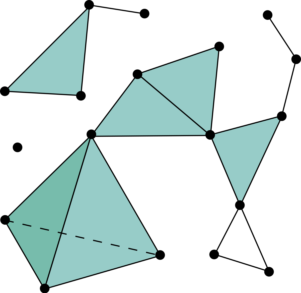
As well as simplices, simplicial complexes can also be actual geometric objects in some Euclidean space, or more abstract, purely combinatorial objects. These two conceptions (geometric vs. combinatorial or abstract) are equivalent, both connected by the notions of geometric realization and scheme: for every abstract -dimensional simplicial complex we may build a geometric simplicial complex (its geometric realization) in , and from every geometric simplicial complex we get the abstract simplicial complex (its scheme) given by the sets of vertices of its simplices. For the sake of briefness, we will be focusing on abstract simplicial complexes only. We recall that throughout the whole text, denotes the -dimensional Euclidean space, in which we consider the usual (Euclidean) distance between two points, given by the length of the straight line segment joining them.
Simplicial complexes are important in our context because of two main reasons:
- •
We can encode chords (vertical events) as simplicial complexes in different ways (see section 1.3) that let us describe a fragment of a music score in terms of their homological invariants (see below).
- •
Simplicial complexes are the basis for topological data analysis, in which simplicial complexes are built (in different ways) from points representing data in a metric space, in relation to their distance (in our case, the Euclidean distance in some ). This construction yields a filtration of simplicial complexes (in our case, the Vietoris-Rips filtration) whose vertices are these data points. This filtration lets us have a homological description of the topological “shape” of the given representation of the data through different “levels”: its persistent homology.
Formally, we have the following (most is taken from Edelsbrunner, Harer et al. 2008):
Definition 2.1.
An (abstract) simplicial complex is a finite collection of sets such that and implies . The sets in are referred to as its simplices, the union of which makes up its set of vertices. To explicitly refer to the vertices of a simplex we write , and we say that span . The dimension of a simplex is given by , where denotes the cardinality of . A simplex on vertices has dimension , and is called an -simplex. The dimension of a simplicial complex is the maximum dimension of any of its simplices. A non-empty subset is called a face of . Note that from the definition, a simplicial complex contains all the faces of its simplices. In the case of geometric simplicial complexes, in addition to this, simplices must be assembled together along their faces.
For simplicial complexes, we have a way of algebraically encoding its shape, by describing its boundary as a formal sum of its simplices and their faces. A simplex together with a fixed order of its vertices is called an oriented simplex. We introduce the boundary operator, denoted by , which is defined on every oriented simplex and then linearly extended to the graded abelian group (or vector space) of formal sums of simplices
where is the group with basis , the set of simplices of dimension . The boundary operator is defined as follows, for each -simplex :
where denotes the -simplex on vertices . By linear extension, this defines a sequence of homomorphisms (respectively, linear functions)
which has the property that for every . Thus, we may define the -th homology group of simplicial complex as the quotient group (resp. vector space)
Homology groups somehow capture the way simplices are “glued” together to form a simplicial complex. They give a rough description of the shape of a space by measuring how many -dimensional “holes” or “voids” are enclosed by it. This is summarized by the ranks or dimensions of the homology groups, called the Betti numbers of , and denoted by These numbers constitute a family of important homotopical invariants of a topological space, and are summarized in the Euler characteristic, given by their alternated sum:
Betti numbers are central in topological data analysis, particularly in persistent homology. Persistent homology is the computation of homological features (namely, Betti numbers) at different “levels”, “scales” or “resolutions” to get an algebraic description of the shape of a set of points in a space. This leads to consider filtrations (another crucial concept in persistent homology). A filtration of a simplicial complex is a sequence of simplicial subcomplexes
We restrict ourselves to finite filtrations.
We consider a one-paremeter filtration of simplicial complexes built upon the points in (taken as vertices). This parameter, usually , establishes the level or scale of scope on the data.
where is the simplex on all points in and . Simplicial complexes in the filtration can be defined according to different constructions. There are different ways to associate a filtration of simplicial complexes with a set of discrete points in a metric space. Persistent homology consists of computing the Betti numbers (which count -dimensional holes or voids) of the simplicial complexes in the filtration considered.
Now we present one particular filtration that can be associated with any cloud of data points in a metric space, the Vietoris-Rips filtration, one of the most commonly used for computing persistent homology, and the one incorporated by the Python library used in this work.
Given a metric space and a finite set of points in X, for each given distance we consider the Vietoris-Rips simplicial complex
is the simplicial complex whose simplices consist of those subsets of points in which are not further than among themselves. So simplices in this case represent “closeness” of points: a -simplex is formed whenever points can be enclosed together in a -ball of radius . As the parameter varies, we obtain a filtration of simplicial complexes, called the Vietoris-Rips filtration, in which the last element is the -dimensional simplex on all vertices of . Figure 28 illustrates this definition.

The Betti numbers of the simplicial complexes in this filtration are computed to obtain a homological description of the “shape” of our cloud of points in space at different scales. They are usually summarized in two graphic ways: persistent barcode graphs and persistent diagrams. These barcodes and diagrams (see figures in section 1.2) record the changing values of the Betti numbers throughout the Vietoris-Rips filtration, and so give us a way of visualizing at which scales do connected components and -dimensional voids appear (their birth, ) and disappear (their death, ). Barcodes are plotted as a set of line segments in the plane , starting and ending at the values of for which each homological feature persists. Similarly, persistence diagrams show the points in the plane , usually plotted alongside the diagonal (all points sit above this line). From this information, certain conclusions about the general distribution of the given points can be drawn, which help in understanding and classifying large collections of data. For example, the longest barcodes are interpreted as the most relevant (persistent) features of the point cloud’s shape.
Barcodes and persistence diagrams corresponding to different sets of points can be compared in several ways. One of the most common is the bottleneck distance, usually denoted (in relation to the family of Wasserstein metrics). This consists of finding a pairing between points in both diagrams, minimizing the maximum possible -distance between corresponding points in the pairing. Formally, the bottleneck distance between diagrams is given by
where ranges over all bijections between and , and
Whenever there is no bijection between and , a partial pairing is considered, and those remaining points are paired with their projection over the diagonal. This metric has the property that it is the least number such that one can draw on the plane squares of side centered at the elements of , and these will also contain the corresponding points of under the matching that defines . Figure 29 shows how points in two different persistence diagrams are matched in order to compute their bottleneck distance. Distances taken among several persistence diagrams can be plotted in a dendrogram (see section 2), which facilitates visualization and comparison of the values obtained for several samples.


Finally, we include the plots of barcodes for mappings III-VI (only harmonic data), corresponding to fragments from several scores (figures 30-34). From looking at the illustrations we can tell there are some distinctive features in the barcode diagrams of samples from different music styles. We can also see the difference in the overall shape of barcodes resulting from mappings III and IV (forming straight blocks), against barcodes corresponding to mappings V and VI (irregular staggered and jagged shapes). In addition, we point out how barcodes for mappings III and V seem to simplify features arising from mappings IV and VI, respectively. In-depth comparison and analysis of particular examples belonging to diverse genres, styles or traditions will be discussed thoroughly in future works.


No potential conflict of interest was reported by the authors.
ORCID
Do not change this. Production will take care of it if the paper is accepted.
References
- Agustín-Aquino et al. (2009) Agustín-Aquino, Octavio A, Janine du Plessis, Emilio Lluis-Puebla, and Mariana Montiel. 2009. “Una introducción a la Teoría de Grupos con aplicaciones en la Teoría Matemática de la Música.” CDMX: Sociedad Mexicana de Matemáticas .
- Andreatta (2003) Andreatta, Moreno. 2003. “Méthodes algébriques dans la musique et la musicologie du XXeme siecle: aspects théoriques, analytiques et compositionnels.” Ph.D. thesis, Ecole des Hautes Etudes en Sciences Sociales (EHESS).
- Beltramo et al. (2021) Beltramo, Gabriele, Rayna Andreeva, Ylenia Giarratano, Miguel O Bernabeu, Rik Sarkar, and Primoz Skraba. 2021. “Euler characteristic surfaces.” arXiv preprint arXiv:2102.08260 .
- Beran and Mazzola (1999) Beran, Jan, and Guerino Mazzola. 1999. “Analyzing Musical Structure and Performance—A Statistical Approach.” Statistical Science 14 (1): 47–79.
- Bergomi (2015) Bergomi, Mattia Giuseppe. 2015. “Dynamical and topological tools for (modern) music analysis.” Ph.D. thesis, Università degli Studi di Milano; Université Pierre et Marie Curie.
- Bergomi and Baratè (2020) Bergomi, Mattia G, and Adriano Baratè. 2020. “Homological persistence in time series: an application to music classification.” Journal of Mathematics and Music 14 (2): 204–221.
- Bergomi, Baratè, and Di Fabio (2016) Bergomi, Mattia G, Adriano Baratè, and Barbara Di Fabio. 2016. “Towards a topological fingerprint of music.” In International Workshop on Computational Topology in Image Context, 88–100. Springer.
- Bigo and Andreatta (2016) Bigo, Louis, and Moreno Andreatta. 2016. “Topological structures in computer-aided music analysis.” In Computational music analysis, 57–80. Springer.
- Bigo and Andreatta (2019) Bigo, Louis, and Moreno Andreatta. 2019. “Filtration of pitch-class sets complexes.” In International Conference on Mathematics and Computation in Music, 213–226. Springer.
- Bigo et al. (2013) Bigo, Louis, Moreno Andreatta, Jean-Louis Giavitto, Olivier Michel, and Antoine Spicher. 2013. “Computation and visualization of musical structures in chord-based simplicial complexes.” In International Conference on Mathematics and Computation in Music, 38–51. Springer.
- Bigo, Giavitto, and Spicher (2011) Bigo, Louis, Jean-Louis Giavitto, and Antoine Spicher. 2011. “Building topological spaces for musical objects.” In International Conference on Mathematics and Computation in Music, 13–28. Springer.
- Bubenik and Dłotko (2017) Bubenik, Peter, and Paweł Dłotko. 2017. “A persistence landscapes toolbox for topological statistics.” Journal of Symbolic Computation 78: 91–114.
- Bubenik et al. (2015) Bubenik, Peter, et al. 2015. “Statistical topological data analysis using persistence landscapes..” J. Mach. Learn. Res. 16 (1): 77–102.
- Deng and Duzhin (2022) Deng, Ran, and Fedor Duzhin. 2022. “Topological Data Analysis Helps to Improve Accuracy of Deep Learning Models for Fake News Detection Trained on Very Small Training Sets.” Big Data and Cognitive Computing 6 (3): 74.
- Edelsbrunner, Harer et al. (2008) Edelsbrunner, Herbert, John Harer, et al. 2008. “Persistent homology -A survey.” Contemporary mathematics 453: 257–282.
- Estrada (2011) Estrada, Julio. 2011. “La teoría d1, MúSIIC-Win y algunas aplicaciones al análisis musical: Seis piezas para piano, de Arnold Schoenberg.” In Memoirs of the Fourth International Seminar on Mathematical Music Theory, Vol. 4Vol. 4, 113–145.
- Giavitto and Spicher (2016) Giavitto, Jean-Louis, and Antoine Spicher. 2016. “A topological approach of musical relationships.” In Mathemusical Conversations: Mathematics and Computation in Music Performance and Composition, 283–298. World Scientific.
- Hatcher (2002) Hatcher, Allen. 2002. Algebraic topology. Cambridge: Cambridge Univ. Press. https://cds.cern.ch/record/478079.
- Jen-Yu, Shyh-Kang, and Yi-Hsuan (2016) Jen-Yu, Liu, Jeng Shyh-Kang, and Yang Yi-Hsuan. 2016. “Applying topological persistence in convolutional neural network for music audio signals.” arXiv preprint arXiv:1608.07373 .
- Mazzola (2012) Mazzola, Guerino. 2012. The topos of music: geometric logic of concepts, theory, and performance. Birkhäuser.
- Padilla et al. (2017) Padilla, Pablo, Francis Knights, Adrián Tonatiuh Ruiz, and Dan Tidhar. 2017. “Identification and evolution of musical style I: Hierarchical transition networks and their modular structure.” In International conference on mathematics and computation in music, 259–278. Springer.
- Pareyón (2011) Pareyón, Gabriel. 2011. On Musical Self-Similarity: Intersemiosis as Synecdoche and Analogy. Gabriel Pareyón.
- Park, Hwang, and Yang (2022) Park, Sungjoon, Yoonseok Hwang, and Bohm-Jung Yang. 2022. “Unsupervised learning of topological phase diagram using topological data analysis.” Physical Review B 105 (19): 195115.
- Rotman (2013) Rotman, Joseph J. 2013. An introduction to algebraic topology. Vol. 119. Springer Science & Business Media.
- Sassone et al. (2022) Sassone, Luca, Marco Manetti, Mattia G Bergomi, and Massimo Ferri. 2022. “Bridging Topological Persistence and Machine Learning for Music Information Retrieval.” .
- Sethares and Budney (2014) Sethares, William A, and Ryan Budney. 2014. “Topology of musical data.” Journal of Mathematics and Music 8 (1): 73–92.
- Straus (2016) Straus, Joseph N. 2016. Introduction to post-tonal theory. WW Norton & Company.
- Szeto and Wong (2006) Szeto, Wai Man, and Man Hon Wong. 2006. “A graph-theoretical approach for pattern matching in post-tonal music analysis.” Journal of New Music Research 35 (4): 307–321.
- Tymoczko (2010) Tymoczko, Dmitri. 2010. A geometry of music: Harmony and counterpoint in the extended common practice. Oxford University Press.