Gaussian mixture modeling of nodes in Bayesian network according to maximal parental cliques
Abstract
To capture the close relevance among nodes in Bayesian network, we take every clique in the network as a cluster, and construct Gaussian mixture model (GMM) on each node according to branches of its maximal parental cliques (MPCs). The definition and finding algorithm for MPCs are presented, accordingly. For the model of GMM-MPC, we targetedly propose an optimization algorithm to train the model parameters. Along with these algorithms, some theoretical analysis are further made to establish strong support. At the end, in experiments we use three public data sets to verify the effectiveness of our proposed method.
1 Introduction
Bayesian network (BN) is a kind of probabilistic graphical models (PGMs) (Koller and Friedman 2009) that uses a graph to represent the joint distribution of a data set and the conditional independence in this distribution. Mathematically, it can be viewed as a directed acyclic graph (DAG), denoted by with to indicate the set of vertexes or nodes and to be the set of directed edges. Every node in the network is usually to represent a random variable while every directed edge measures conditional dependencies between the connected two nodes. Due to having clear structure and strong interpretability, BN has been widely used in many respects, including medical diagnosis (Glymour et al. 2016), product recommendation (Ono et al. 2007), images and sentences generation (Dethlefs and Cuayáhuitl 2011; Kingma and Welling 2019), etc.
As a graphic model, the performance of BN depends on both the graphic structure and the distribution used to model the nodes. A “good" BN thus needs to learn the network structure and the distribution (including the distribution form and parameters), respectively. For the former, the learning algorithms include constraint-based algorithms (Colombo et al. 2014; Spirtes et al. 2000) that measure the conditional independencies through independence tests, score-based algorithms that use a score function to rank the graph and find the graph with highest score, such as greedy equivalence search (GES) (Chickering 2002) and greedy interventional equivalence search (GIES) (Hauser and Bühlmann 2012), and their hybrid methods, like max-min hill climbing (MMHC) algorithm (Tsamardinos et al. 2006). For the distributions used in BN, as far as continuous data is concerned, the most frequently-used one is the linear Gaussian distribution. Based on it, some improved versions and other distributions have been also reported for the purpose of strengthening the performance of BN. The well-known Variational AutoEncoder (Kingma and Welling 2013) uses deep neural networks to model the mean of the linear Gaussian model. Harris and Drton (Harris and Drton 2013) proposed the nonparanormal distribution instead, which uses different strictly increasing functions to act on the normal distribution as the new distribution. Song et al. (Song et al. 2011) used nonparametric representation as distribution, and Radu-Stefan et al. (Niculescu et al. 2006) imposed expert knowledge on constraining the parameters of the linear Gaussian distribution.
The above improvements on model strengthen greatly the generative and discriminative abilities of BN, but the resulting models have too complex structures that are difficult to understand so as to cause loss of interpretability. For this reason, we try to use the Gaussian mixture model (GMM, a weighted average of finite Gaussian distribution) (McLachlan and Basford 1988) in BN, which has transparent meaning on every parameter and thus can keep interpretability. Naturally, it is not the first time to apply GMM to model BN. Roos et al. applied GMM on dynamic BN to predict the passenger flow (Roos et al. 2017), and Monti et al. used GMM on naive BN to perform classification task of discrete data (Monti and Cooper 2013). However, these applications rely on special graphic structure of BN, such as dynamic BN or naive BN, and moreover, for every node GMM takes all of its parent nodes as a branch and is equipped with the same number of branches. These fixed settings may restrict the performance of the PGM combing BN and GMM. We thus study a very general case with no limitations on the structure of BN or on the number of branches in GMM. To capture the close relations among nodes, we utilize the clique structure (a cluster of nodes with any two nodes connected) and model every node with GMM according to its maximal parental clique (MPC), referred to as GMM-MPC in the context. A new optimization algorithm called double iteration optimization (DIO) algorithm is further proposed to optimize GMM-MPC with conditional variables in every branch under equality constraint. We finally use three data sets to test our models and algorithms.
The rest of the paper is organized as follows. Section 2 introduces some background knowledge about BN and GMM. Section 3 shows the modeling framework of GMM-MPC in BN, including definition of MPC, DIO algorithm and some theoretical analysis. Then, some experiments and discussions are given in Section 4. Finally conclusion and other thinking are presented in Section 5.
2 Preliminaries
In this section, we will make a brief introduction on BN and GMM.
2.1 Bayesian network
Consider a BN . If and , then we call is a parent of , denoted by , and is a child of , denoted by . There are three basic structure in BN: chain (), fork () and v-structure (), where . In the v-structure, the middle node is defined as collider. If the parents of collider are disconnected, we say this v-structure is immorality. However, if a v-structure is not immorality, it is a complete subgraph and all the nodes in it can be colliders, so we call collider we mean the collider in immoralities.
For a set of nodes , if any pair of nodes in have an edge, is called a clique. Further, if there is no clique in graph such that , then is the maximal clique in . If a graph is a clique, we call this graph complete graph. All the complete graphs who have same nodes are I-equivalent since there is no conditional independencies.
Different graphs can represent the same distribution as long as they have the same nodes and conditional independencies, we call these DAG are I-equivalentChickering 2013.
Thus most of the structure learning algorithms return a partially directed acyclic graph which can become all I-equivalent DAGs that represent the same distribution of data by changing all the undirected edges to arbitrary directed edgesChickering 2013.
The values of nodes only depend on the parents of them and some Gaussian noises. The decomposition of a joint distribution is
The most widely used distribution in BN is linear Gaussian , where is the value of , and , and are learnable parameters. Different structures of graph have different decomposition, thus have different conditional independencies, so a good structure learning algorithm can definitely improve the generative ability of BN. We do our experiments based on different structure learning algorithms.
2.2 Gaussian mixture model and expectation maximization algorithm
GMM is the weighted average of finite Gaussian distribution,
| (1) |
with restriction , where each Gaussian distribution is called a branch or component, and , and are the mean, variance and coefficient in k-th cluster. If the data set appears to have more than one clusters and a single Gaussian model is hard to fit the joint distribution, GMM uses its every branch to approximate every cluster of data. (figure 1 (a))
We set the Lagrange function as the loss function where is the Lagrange multiplier. Setting the derivatives of the loss function with respect to the , and for k=1,2,…,K, we obtain and
| (2) |
where and Bishop and Nasrabadi 2006. EM algorithm has E-step and M-step in every epoch, In E-step, EM takes the , and from the last epoch to compute for and , in M-step it uses the data and to compute and in equation (2), and takes and as inputs to obtain . EM algorithm continues this routine until loss function converges.
3 GMM framework
In this section, we will give the definition of MPC, the searching algorithm for it, and the Gaussian mixture modeling framework on node according to its MPCs.
3.1 MPC
Intuitively, the connection among nodes in a clique of BN is stronger than that in other set of nodes, since there is an edge between any pair of nodes. Cliques tree inference (Kjærulff 1998) utilizes this point and takes each clique as a cluster, passing information from one clique to another to obtain the marginal distributions. Inspired by this operation, we also model BN by taking every clique as a cluster, and for every node in clique we construct a GMM with every branch corresponding to one of its MPCs. Here, we only consider the cliques in , the main reason of which is that the value of only depends on its parents. The MPC is defined as follows.
Definition 1.
Given a BN , for any if the clique and no other such that , then is called a maximal parental clique of .
To construct GMM for node , it is necessary to find all of its maximal parental cliques. From the definition, we can find that if a clique and is a maximal clique, then is a MPC of . Namely, the MPCs of are in , which means that can be written as with to represent every MPC.(figure 1 (b)) Clearly, comes from a clique of , while the elements in clique might belong to and/or , so we introduce an important notation serving for developing algorithm to find the MPCs of node .
In Algorithm 1, the of all nodes in can be obtained by graphic structure learning algorithms, like MMHC, etc. Line 2 goes through all arrangements of nodes in with the purpose of finding all combinations of and nodes in to avoid getting only one clique given a kind of arrangement. Line 5 depends on the fact that a clique after adding another new node is still a clique if and only if this clique is in . Meanwhile, to ensure this clique is a MPC, we need to check every node in this clique is parent of . However, it is still possible to get the same clique from different arrangements, so we check the repetition in Line 9. The output is the set of all MPCs.
3.2 GMM of node according to branches of its MPC


Consider a data set , where is the number of instances and . Let represent the th feature variable of , corresponding to the th node in the assigned BN . Then, the GMM for node is written as
| (3) |
where is the number of branches (every MPC acts for a branch), is the weighted coefficient of the th MPC constrained by , is the th MPC of , and is the component distribution of given . By taking the conditional distribution in (3) as the posterior distribution, and the marginal distribution of node as the prior distribution, we have
Theorem 1.
If the component distributions in (3) are conjugate distributions, then the mixture distribution there is also a conjugate distribution. Moreover, the joint distribution of the graph is a mixture distribution i.e. , where is the number of clusters of joint distribution and .
Note that the left side of (3) is certainly seen as a mixture distribution, but the component distribution in the right side can be also seen as a mixture model which has only one cluster. Similarly, it applies to the distributions of every subgraph. We put the detailed proof in the Appendix.
We say a graph is a perfect map to data set if have all the conditional independencies in . Using Theorem 1, we have the following theorem.
Theorem 2.
Let be a perfect map, then the marginal distribution of a node in is a mixture distribution with more than one components if and only if the node is a collider or the descendant of a collider.
In the Appendix, we prove only the collider and its descendants can have more than one MPCs. However, in the perfect graph the reverse is also true since if the coefficient of a MPC of the collider is zero, then the nodes in MPCs have no impact on . That is to say they are not parents of which contradicts to the definition of the perfect map.
We consider the component distributions as linear Gaussian model, similarly, we can obtain the Lagrange function about joint distribution of all nodes in
| (4) |
as loss function, where is the value of i-th nodes in j-th data, is the th MPC of th node in th data, , , , are learnable parameters. Meanwhile, it has n equality constraints. The equation (4) can be seen as a likelihood function of n GMM-MPCs, but the mean of equation (1) are learnable parameters, and the mean of (4) contains some features of data.
lemma 1.
To achieve the minimum of equation (4), , and update equation in EM algorithm with respect to equation (4) is
| (5) | ||||
| (6) | ||||
| (7) |
where .
We can find that the equation of biases and variances replace the in equation (2) with the linear function. The proof of these equations can be found in Appendix. However the weights can not be obtained in the same way since they multiply by the value of maximal parental clique which is related to the data set. The restriction is a hard constraint(Boyd et al. 2004) which is required to make equation (3) a distribution so the gradient descent optimization can not optimize equation (4). We may use softmax function on for k=1,…,, or normalize each of by dividing sum of them after certain epochs, but this can not guarantee the local optimum. So we propose the double iteration optimization(DIO), Algorithm 2 gives details of it.

An outer epoch in DIO has two part, DIO uses the equation (7) to compute the coefficient in the first part, then fixes them and uses any kinds of gradient descent optimization to minimize the loss function in the second part in line 17, we use the mini-batch technique to accelerate the process.
Theorem 3.
The double iteration optimization has hill-climbing property, if the inner epoch is big enough, then it will reach the local optimum.
The latter part of Theorem 3 is trivial since DIO reaches a local optimum after every outer epoch for a big enough inner iteration. But in first part of outer epoch, it updates all the coefficients in last outer epoch, because of its hill-climbing property, the loss function reaches a smaller value than the local optimum at the end of last outer epoch, it can reaches a much smaller local optimum at the end of this outer epoch(figure 2). The complete proof is in Appendix
Notice that the mean and variance of Gaussian distribution can be more general form like in VAE, the weights in mixture model of this form is completely intractable, but we still can use DIO in this case. Moreover, we can not only update the coefficient in first part of outer epoch, but also update the biases and variances if they can be derived by the similar way in equation (6).
The drawback of DIO is obvious. In line 8, we need to use all the data set to update the coefficient which needs a lot of time and resource. If we also update the variances or biases in first part of outer epoch, it costs much more resource since variances and biases are more complicated to compute. Although in each outer epoch, the loss can reach a smaller local optimum, it can not reach the global optimum after enough outer epochs, the update of coefficients only makes the current local optimum ’deeper’ with respect to the weights, not finds a another smaller local optimum(Figure 2).
4 Experiments
In this section, we make some numerical experiments to exhibit the effectiveness of GMM-MPC. Three publicly-available data sets, Mental health (Jain), House (Holbrook) and Sachs (Sachs et al. 2005), are used. The basic information about them are given in Table 1. Here, we are only concerned with continuous features, and the discrete features are removed from data sets. We do experiments on CPU i7-12700H, and all codes and part of data sets are provided in the Supplemental material.
| Data sets | Continuous | Number of | Mini-batch |
|---|---|---|---|
| Features | Instances | Size | |
| Mental health | 12 | 125000 | 10000 |
| House | 9 | 20640 | 7000 |
| Sachs | 11 | 7466 | 3000 |
We first learn the graph structures of data sets. In this paper, three kinds of existing methods are directly borrowed, including PC (Colombo et al. 2014), MMHC (Tsamardinos et al. 2006) and greedy search (GS) (Margaritis 2003) algorithms. The main purpose is to evaluate the performance of the proposed GMM-MPC under different graph structures. After performing normalization, we train the graph structure of every data set, and the results are exhibited in Figures 4, 5 and 6 in Supplement. We also present the corresponding number of edges in each graph structure in Tables 2, 3 and 4. Based on these results, Algorithms 1 and 2 are further applied to find MPCs for every node and optimize the model parameters, respectively. In the training process, Adam (Kingma and Ba 2014) is selected as the gradient descent method for DIO, and the learning rate is set as . The initial weights, bias and all of variances are set as 0, 0 and 1, respectively. We use -fold cross validation to perform training on each data set. The training stops just before overfitting, which is implemented by an early stopping technique. This technique allows model testing to be done simultaneously after a certain amount of trainings, and identifies overfitting through observing the testing accuracy change. The overfitting corresponds to the time at which the testing accuracy begin to become low. At the moment, the number of training is called epochs. We use the average minus log-likehood as a criterion to evaluate the testing accuracy, and write down epochs in the form of and testing accuracy in the form of , with the results also reported in Tables 2, 3 and 4. Additionally, considering the increasing parameters in introducing mixture models, we select the Bayesian information criterion (BIC)(Neath and Cavanaugh 2012) to balance the model accuracy and complexity, defined by
| (8) |
Here, is the log-likelihood function, represents parameters, is the number of model parameters and is the number of testing instances. The results of BIC are provided in those three tables as well.
| Model | Structure | Number of | Epochs | Number of | Average Minus | BIC |
|---|---|---|---|---|---|---|
| Learning | Edges | Parameters | Log-Likelihood | |||
| LG | PC | 11 | 200 | 35 | 18.250.056 | 4564961287 |
| GMM | PC | 11 | 206 | 99 | 17.960.04 | 449515914 |
| GMM-MPC | PC | 11 | 204 | 49 | 17.900.03 | 44781069 |
| LG | MMHC | 32 | 320 | 56 | 17.180.13 | 4297983062 |
| GMM | MMHC | 32 | 207 | 190 | 17.480.41 | 43802810144 |
| GMM-MPC | MMHC | 32 | 206 | 115 | 17.060.02 | 42707156 |
| LG | GS | 31 | 240 | 55 | 17.710.04 | 4428271039 |
| GMM | GS | 31 | 207 | 194 | 18.380.08 | 4605511903 |
| GMM-MPC | GS | 31 | 204 | 108 | 17.400.02 | 43550026 |
| Model | Structure | Function | Number of | Epochs | Number of | Likelihood | BIC |
|---|---|---|---|---|---|---|---|
| Learning | Edges | Parameters | Score | ||||
| LG | PC | Linear | 6 | 100 | 24 | 14.210.26 | 587531055 |
| GMM | PC | Linear | 6 | 1510 | 71 | 11.662.10 | 484308667 |
| GMM-MPC | PC | Linear | 6 | 1510 | 28 | 10.410.24 | 43084977 |
| LG | MMHC | Linear | 18 | 110 | 36 | 15.450.09 | 63947387 |
| GMM | MMHC | Linear | 18 | 1510 | 121 | 10.941.74 | 454017186 |
| GMM-MPC | MMHC | Linear | 18 | 1510 | 53 | 10.251.19 | 425514893 |
| LG | GS | Linear | 15 | 120 | 33 | 16.670.69 | 689412858 |
| GMM | GS | Linear | 15 | 1510 | 112 | 11.143.03 | 4644112503 |
| GMM-MPC | GS | Linear | 15 | 1510 | 58 | 10.552.32 | 437839556 |
| LG | PC | Sigmoid | 6 | 70 | 24 | 13.160.02 | 5443298 |
| GMM-MPC | PC | Sigmoid | 6 | 2010 | 28 | 10.431.50 | 431906173 |
| LG | MMHC | Sigmoid | 18 | 70 | 36 | 13.170.07 | 54522276 |
| GMM-MPC | MMHC | Sigmoid | 18 | 2010 | 53 | 10.301.48 | 427456117 |
| LG | GS | Sigmoid | 15 | 70 | 33 | 13.180.06 | 54530249 |
| GMM-MPC | GS | Sigmoid | 15 | 2010 | 58 | 10.261.54 | 425996373 |
| Model | Structure | Function | Number of | Epochs | Number of | Likelihood | BIC |
|---|---|---|---|---|---|---|---|
| Learning | Edges | Parameters | Score | ||||
| LG | PC | Linear | 10 | 90 | 32 | 16.831.19 | 252501771 |
| GMM | PC | Linear | 10 | 205 | 94 | 14.090.29 | 21378430 |
| GMM-MPC | PC | Linear | 10 | 204 | 37 | 13.220.95 | 198781421 |
| LG | MMHC | Linear | 27 | 100 | 49 | 22.581.00 | 338891498 |
| GMM | MMHC | Linear | 27 | 205 | 166 | 15.662.77 | 239874141 |
| GMM-MPC | MMHC | Linear | 27 | 205 | 68 | 13.901.42 | 210072125 |
| LG | GS | Linear | 31 | 90 | 53 | 21.560.76 | 323791131 |
| GMM | GS | Linear | 31 | 205 | 178 | 13.871.19 | 213521773 |
| GMM-MPC | GS | Linear | 31 | 205 | 118 | 12.250.91 | 187191365 |
| LG | PC | Sigmoid | 10 | 60 | 32 | 15.790.27 | 23688402 |
| GMM-MPC | PC | Sigmoid | 10 | 204 | 37 | 13.210.50 | 19853747 |
| LG | MMHC | Sigmoid | 27 | 60 | 49 | 15.640.45 | 23531668 |
| GMM-MPC | MMHC | Sigmoid | 27 | 205 | 68 | 12.840.94 | 194251407 |
| LG | GS | Sigmoid | 31 | 50 | 53 | 15.590.28 | 23471416 |
| GMM-MPC | GS | Sigmoid | 31 | 205 | 118 | 12.810.62 | 19563934 |
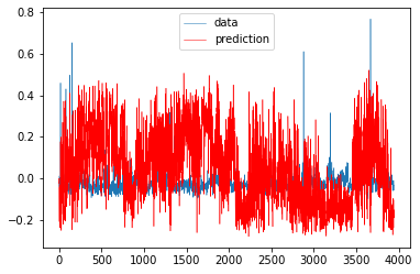
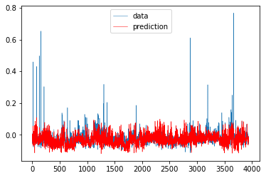
To fully exhibit the effectiveness of GMM-MPC, we simultaneously select another two models, linear Gaussian (LG) model and ordinary GMM Roos et al. 2017; Monti and Cooper 2013; Liu 2012 where each node is set to have the same number of branches, 3, in all experiments, for comparisons. The corresponding experimental results are also shown in Tables 2, 3 and 4. For the latter two data sets, we compare three kinds of models. Moreover, we change the mean of Gaussian distributions with more complicated function (from Linear function to Sigmoid function ) to indicate that GMM-MPC can also have improvement on more general form of distribution, i.e., As can be seen from these tables, GMM-MPC completely outperform the other two models according to average testing accuracy and BIC whatever the graph structure (PC, MMHC or GS) is and whatever the function (linear or Sigmoid one) is. We also notice that ordinary GMM has much more parameters than GMM-MPC, but still has worse performance than GMM-MPC. According to the Algorithm 2, the number of increased parameters is with to represent the number of maximal parental cliques of . However in ordinary GMM, it is where is a hyperparameter. Figure 3 displays the prediction results of GMM-MPC and LG models with Sigmoid function on House data set. The former exhibit much more prediction power than the latter.
5 Conclusion
We use the mixture model on the Bayesian network based on the maximal parental cliques and propose a new optimization method DIO to find the local optimum of loss function. GMM-MPC can increase the generative and discriminative ability dramatically as we see in the tables and figure 3. More importantly, we can understand the meaning of every parameters i.e. the weights decide the influence of parents of nodes, the coefficients show how each cluster influences the prediction of target node, thus the iterpretability of BN remains. GMM-MPC may increase the number of parameters compare to LG, but this increase is acceptable under the concept of BIC and it has much less parameters than GMM. However in the training process, vanishing gradient and exploding gradient may appear, because unlike the log-likelihood function of LG, equation (4) puts mixture models in the . Also in tables, we can find training GMM-MPC in BN always needs more epochs, e.g. in table 2, we train a LG with ’Sigmoid’ only needs 70 epochs, but we need 200 epochs to train a GMM-MPC with ’Sigmoid’. These may be some points of our future efforts.
References
- Bishop and Nasrabadi [2006] Christopher M Bishop and Nasser M Nasrabadi. Pattern recognition and machine learning, volume 4. Springer, 2006.
- Boyd et al. [2004] Stephen Boyd, Stephen P Boyd, and Lieven Vandenberghe. Convex optimization. Cambridge University press, 2004.
- Chickering [2002] David Maxwell Chickering. Optimal structure identification with greedy search. The Journal of Machine Learning Research, 3(Nov):507–554, 2002.
- Chickering [2013] David Maxwell Chickering. A transformational characterization of equivalent bayesian network structures. arXiv preprint arXiv:1302.4938, 2013.
- Colombo et al. [2014] Diego Colombo, Marloes H Maathuis, et al. Order-independent constraint-based causal structure learning. The Journal of Machine Learning Research, 15(1):3741–3782, 2014.
- Dethlefs and Cuayáhuitl [2011] Nina Dethlefs and Heriberto Cuayáhuitl. Combining hierarchical reinforcement learning and bayesian networks for natural language generation in situated dialogue. In Proceedings of the 13th European Workshop on Natural Language Generation, pages 110–120, 2011.
- Glymour et al. [2016] Madelyn Glymour, Judea Pearl, and Nicholas P Jewell. Causal inference in statistics: A primer. John Wiley & Sons, 2016.
- Harris and Drton [2013] Naftali Harris and Mathias Drton. Pc algorithm for nonparanormal graphical models. The Journal of Machine Learning Research, 14(11), 2013.
- Hauser and Bühlmann [2012] Alain Hauser and Peter Bühlmann. Characterization and greedy learning of interventional markov equivalence classes of directed acyclic graphs. The Journal of Machine Learning Research, 13(1):2409–2464, 2012.
- [10] Ryan Holbrook. Dl course data. https://www.kaggle.com/datasets/ryanholbrook/dl-course-data?select=housing.csv. Accessed November 4, 2021.
- [11] Gaurav Jain. Mobile health human behavior analysis. https://www.kaggle.com/datasets/gaurav2022/mobile-health. Accessed March 11, 2022.
- Kingma and Ba [2014] Diederik P Kingma and Jimmy Ba. Adam: A method for stochastic optimization. arXiv preprint arXiv:1412.6980, 2014.
- Kingma and Welling [2013] Diederik P Kingma and Max Welling. Auto-encoding variational bayes. arXiv preprint arXiv:1312.6114, 2013.
- Kingma and Welling [2019] Diederik P Kingma and Max Welling. An introduction to variational autoencoders. arXiv preprint arXiv:1906.02691, 2019.
- Kjærulff [1998] Uffe Kjærulff. Inference in bayesian networks using nested junction trees. In Learning in Graphical Models, pages 51–74. Springer, 1998.
- Koller and Friedman [2009] Daphne Koller and Nir Friedman. Probabilistic graphical models: principles and techniques. MIT press, 2009.
- Liu [2012] Hui Liu. Bayesian networks and gaussian mixture models in multi-dimensional data analysis with application to religion-conflict data. Technical report, Arizona State University, 2012.
- Margaritis [2003] Dimitris Margaritis. Learning bayesian network model structure from data. Technical report, Carnegie-Mellon Univ Pittsburgh Pa School of Computer Science, 2003.
- McLachlan and Basford [1988] Geoffrey J McLachlan and Kaye E Basford. Mixture models: Inference and applications to clustering, volume 38. M. Dekker New York, 1988.
- Monti and Cooper [2013] Stefano Monti and Gregory F Cooper. A bayesian network classifier that combines a finite mixture model and a naive bayes model. arXiv preprint arXiv:1301.6723, 2013.
- Neath and Cavanaugh [2012] Andrew A Neath and Joseph E Cavanaugh. The bayesian information criterion: background, derivation, and applications. Wiley Interdisciplinary Reviews: Computational Statistics, 4(2):199–203, 2012.
- Niculescu et al. [2006] Radu Stefan Niculescu, Tom M Mitchell, R Bharat Rao, Kristin P Bennett, and Emilio Parrado-Hernández. Bayesian network learning with parameter constraints. The Journal of Machine Learning Research, 7(7), 2006.
- Ono et al. [2007] Chihiro Ono, Mori Kurokawa, Yoichi Motomura, and Hideki Asoh. A context-aware movie preference model using a bayesian network for recommendation and promotion. In International Conference on User Modeling, pages 247–257. Springer, 2007.
- Roos et al. [2017] Jérémy Roos, Stéphane Bonnevay, and Gérald Gavin. Dynamic bayesian networks with gaussian mixture models for short-term passenger flow forecasting. In 2017 12th International Conference on Intelligent Systems and Knowledge Engineering (ISKE), pages 1–8. IEEE, 2017.
- Sachs et al. [2005] Karen Sachs, Omar Perez, Dana Pe’er, Douglas A Lauffenburger, and Garry P Nolan. Causal protein-signaling networks derived from multiparameter single-cell data. Science, 308(5721):523–529, 2005.
- Song et al. [2011] Le Song, Eric Xing, and Ankur Parikh. Kernel embeddings of latent tree graphical models. Advances in Neural Information Processing Systems, 24, 2011.
- Spirtes et al. [2000] Peter Spirtes, Clark N Glymour, Richard Scheines, and David Heckerman. Causation, prediction, and search. MIT press, 2000.
- Tsamardinos et al. [2006] Ioannis Tsamardinos, Laura E Brown, and Constantin F Aliferis. The max-min hill-climbing bayesian network structure learning algorithm. Machine Learning, 65(1):31–78, 2006.
Appendix A Proofs of Theorems
A.1 Proof of Theorem 1
To prove the mixture distributions (3) are all conjugate distributions for i=1,2,..n, we need to prove the prior distributions and posterior distributions are in the same family. Since we define the posterior in (3), we need to obtain the prior distributions of , i=1,2…n.
In DAG , there must be a node has no parent, otherwise must have a cycle. So the prior and posterior distribution of are the form of , can be seen as a mixture distribution whose number of component is one. By using induction method, for posterior distribution of any node , we assume the joint distribution is a mixture distribution i.e.
Then we obtain the joint distribution of and
The last step is using the assumption of theorem that the component distribution is conjugate distribution.Then by eliminating the variables , we have the prior distribution of
where is the set of all possible values of features . From equation above, the is the form the because of the conjugate of , and , so the prior distribution and the posterior distribution are in the same family of distribution, then the mixture distribution is conjugate.Moreover,
where , and so the joint distribution of graph is mixture model. For any subset of nodes , eliminating the rest of nodes in , we know the joint distribution of is the form of
A.2 Proof of Theorem 2
Let us assume node is a collider, by the definition of collider, we can find two parents of : ,, and and . Find any maximal clique that contains , and any maximal clique that contains Y, let and , then , , and are two different maximal parental cliques. The coefficient of these two maximal parental cliques , are non-zero, otherwise if , then is not parent of , since we choice and arbitrarily, then is not a collider, this is contradictory to the assumption.
According to the Theorem 1, we know the joint distribution of is mixture distribution , let the conditional distribution of be , then the marginal distribution of is
There is at least one such that , then in the equation above, and are non-zero, so the marginal distribution of has more than one component.
If is the descendant of collider, without loss of generality we can assume one of the node is collider. From the proof of Theorem 1, where , we know
We assume , then by the proof before, we know conditional distribution has more than one component, without loss of generality, we assume and , then there are at least two non-zero coefficient in and for , . Similarly, the marginal distribution of is
It simply replaces the with , then the marginal distribution of has at least two components.
A.3 Proof of lemma 1
To minimize equation (4), we need to compute the value of Lagrange multiplier , let stands for the equation (4), setting the derivatives of equation (4) with respect to , we have
Multiply on both side and sum all the k from 1 to ,
so for .Thus
which proves the equation (7). We can obtain the derivation of with respect to biases, variances and weights
These derive equation (5) (6)
A.4 Proof of Theorem 3
To prove the hill-climbing property of DIO, we need to prove after every outer epoch, the value 0f loss function (4) is become smaller. In one outer epoch, the inner iteration is gradient descent which is hill-climbing algorithm, we only need to prove the update of coefficients is hill-climbing.
Since in the first part of outer epoch, the weights, biases and variances are constant, we write for short. Let be the coefficients at present and be the coefficients in next outer epoch, then by the Lemma 1,
So , the coefficients satisfy the constraint in every inner and outer epoch.
We use and be the loss function at present and at next outer epoch,
since is convex then
continue the process, we obtain
Appendix B Other details and results in experiments
The details of experiments are shown below.
As we mentioned in the conclusion, GMM in BN may face the vanishing gradient and exploding gradient. To avoid these phenomenons, we add a constant in the in equation (4),
And add the in the update of coefficient in Algorithm 2,
In experiments, we set . Although we apply this measure in experiment, we may still meet vanishing gradient when the training loss become too small, early stopping can completely solve this problem.


