Safety Verification and Controller Synthesis for Systems with Input Constraints

We start the formulation for a continuous-time nonlinear system for generality. The system is described by an ordinary differential equation:

where $x(t)\in\mathbb{R}^{n}$ denotes the state vector, and $u(t)\in\mathcal{U}\subseteq\mathbb{R}^{m}$ is the control input, where $\mathcal{U}$ is a bounded set denoting actuation limits and $f(\cdot,\cdot)$ is a locally Lipschitz continuous vector field. We assume that the solution to (1) is unique. The flow $\psi(x,t,u)$ denotes the solution of (1) at time $t$ from initial condition $x$ under control $u$. The definitions of a reachable set, forward invariance and safety can be extended to the control system setting.

We note here that although the vector field $f(\cdot,\cdot)$ in (1) already includes the control input $u$, we still denote the input explicitly in the subscript to distinguish this from the reachable set $R_{f}^{T}(X)$ for the autonomous system $\dot{x}=f(x)$.

If $u=0$, we call the set $X$ positive invariant. The difference between positive invariance and control invariance is obvious: the control effort allows guaranteeing that the flow stays in the set. Hence, the safety of the control system not only depends on the vector field and the predefined safe set $S$, but also on the control admissible set $\mathcal{U}$.

The definition of safety of a controlled system is similar to that of an autonomous system. To incorporate safety for the nonlinear control system (1), we aim at finding controller $u$ and a control invariant set $W$, which includes $I$ in its interior and is a subset of the safe set $S$. In particular, $W$ and $u$ fulfill:

We now define the notion of Control Barrier Certificates (CBC) for finding a feasible candidate control invariant set, and a controller according to condition (2).

Let

denote the admissible set of control inputs for a CBC $B(x)$. Let $\mathcal{B}:=\{x|B(x)\geq 0\}$ denote the zero-super level set of $B(x)$. We then have the following result on safety.

Theorem 1 shows that the existence of a control Barrier certificate $B(x)$ ensures safety for safety-critical systems. Meanwhile, the control admissible set (4) certifies the selection of control effort. For problems that the control Barrier certificate $B(x)$ can be easily constructed and verified through physical properties, one can formulate a quadratic program to synthesize the safe controller $u$ at $x$.

where $u^{*}(x)$ is a nominal control input designed from other tools, e.g. PID, MPC. We note here the formulation (5) is different from that of CBF based QP. Here, in the interior of the control invariant set $\mathcal{B}$, the solution of (5) is the direct projection from $u^{*}(x)$ on the control admissible set $\mathcal{U}$.

For the scenario where the control Barrier certificate is unknown, the problem is to synthesise the control Barrier certificates together with the safe controller design. To begin with, $B(x)$ is parameterized by

where $p:=\{p_{1},\ldots,p_{k}\}$ denotes a series of parameters which will be decision variables in an optimisation problem, and $\Lambda_{1}(x),\ldots,\Lambda_{k}(x)$ are a class of function basis. The new optimisation problem for constructing the CBC and controller is

Compared to quadratic programming (5) with known control Barrier certificates, (7) is computationally intractable since it involves solving an infinitely constrained optimisation problem. We will show how to address this difficulty by sum-of-squares programming in Section III.

To interpret the constraints (3) into SOS constraints, we assume that the resulting control Barrier certificate is a polynomial function parameterized by real coefficients $p_{1},\ldots,p_{m}$ in the following way

where $b_{j}(x)$s are polynomial or monomial function bases, and $p_{0}$ is a positive real scalar. Similarly, the control input is parameterized by real scalar coefficients $k_{1},\ldots,k_{l}$, and a real vector coefficient $k_{0}\in\mathbb{R}^{m}$ with

where $v_{j}(x)$s are polynomial or monomial vector bases. We note here there the reason why we use the constant term $k_{0}$ is different from that of $p_{0}$. From the view of control, $k_{0}$ introduces a feedforward term, which in some cases is important for safety, for example at some singular points where $\mathop{\sum\limits_{j=1}^{l}k_{j}v_{j}(x)}=0$.

We note that in Theorem 2 we only require a polynomial multiplier $\lambda$, but not a SOS one since the condition $\frac{\partial B(x)}{\partial x}(f(x)+g(x)u(x))\geq 0$ is only imposed on the boundary $B(x)=0$. Condition (12c) introduces products of decision variables, i.e. $\lambda B(x)$, which results in bilinearity. However, there is no guaranteed solver for nonconvex, or specifically bilinear constrained SOS programs. Here, like existing work of using SOS to synthesize Barrier certificates, we use an iterative procedure for control Barrier certificate synthesis and safe control law design. Different from the iterative algorithm for Barrier certificate synthesis, our problem involves an additional polynomial variable $u$ in the SOS program. Thus, an additional round for controller synthesis is required in our algorithm.

1) Initialization: We first fix the degree of polynomials $B(x)$, $\sigma_{\mathrm{safe}}$, $\sigma_{\mathrm{init}}$, $\lambda_{1}$, $\lambda_{2}$ and $u(x)$. The polynomial/monomial scalar/vector bases $b_{j}(x)$s and $v_{j}(x)$s in (10) and (11) have degree upper bounded by the aforementioned degrees of $B(x)$. $\epsilon_{1}$ and $\epsilon_{2}$ are chosen to be small real numbers. Unlike the iterative procedure proposed in [11] which initializes the control law by a scaled LQR controller, we find the initialized feasible control input $u^{0}(x)$ by solving a feasibility SOS program.

We note here that there is no assumed control Barrier certificate $B(x)$ at this stage of finding the initial feasible control input $u^{0}(x)$. Therefore, $u^{0}(x)$ can not be restricted to the domain of $\partial\mathcal{B}$ as that in (12d). Other than directly interpreting $A(k_{0}+\sum_{j=1}^{l}k_{j}v_{j})+b\in\Sigma[x]^{h}$, we add an additional positive multiplier $\sigma_{\mathrm{cont}}$ which satisfies $\sigma_{\mathrm{cont}}-\epsilon_{3}\in\Sigma[x]$, $\epsilon_{3}>0$ to avoid introducing constant terms in the SOS constraints, as well as improving feasibility. The resulting initial controller $u^{0}(x)$ is derived by the parameters $k_{1},\ldots,k_{l}$ and the scaled term $\sigma_{\mathrm{cont}}$ from the solution of (13)

The feasibility of such an initialized controller is guaranteed by the following proposition.

Given initial input $u^{0}(x)$, the corresponding scaled multiplier $\sigma_{\mathrm{cont}}$, the initial control Barrier certificate $B^{0}(x)$ can be found by solving an initial feasibility SOS program as

The boundary condition (12c) is strengthened to be $\frac{\partial B(x)}{\partial x}(f(x)+g(x)u(x))-\epsilon_{2}\in\Sigma[x]$ for convexity and simplicity of computing. This condition is also referred to be the weak Barrier certificate in [7]. $\sigma_{\mathrm{cont}}\cdot\frac{\partial B(x)}{\partial x}(f(x)+g(x)u^{0}(x))-\epsilon_{2}$ is guaranteed to be a polynomial, since $\sigma_{\mathrm{cont}}\cdot u^{0}(x)$ is a polynomial.

After obtaining a feasible initial control input $u^{0}(x)$ and control Barrier certificate $B^{0}(x)$, the problem of control Barrier certificates synthesis can be regarded as a Barrier certificates synthesis problem with vector field $f(x)+g(x)u^{0}(x)$. The multipliers $\lambda_{1}^{0}$, $\lambda_{2}^{0}$ are fixed to be 0 or 1 in initialization for simplicity. The initial control Barrier certificate $B^{0}(x)$ is used to enlarge the size of the control invariant set incrementally. The following steps of the algorithm iteratively solve the SOS program to address the bisecting terms $\lambda_{1}B(x)$ and $\frac{\partial B(x)}{\partial x}(f(x)+g(x)u(x))$ in (12c).

2) Update the control input $u^{k}(x)$: At iteration $k$, given a control Barrier certificate from (15) (when $k=1$) or (17) (when $k\geq 2$), the controller synthesis is constrained to (12d). Fixing $B(x)=B^{k-1}(x)$, a convex programming synthesis procedure for $u^{k}(x)$ is

and we have that $u^{k}(x)=(k_{0}+\sum_{j=1}^{l}k_{j}v_{j}).$ Here we use $\lambda_{1}$ other than $\lambda_{1}^{k-1}$ since $B(x)$ has been substituted by $B^{k}(x)$, thus there is no bilinear term anymore. By limiting the domain of the controller to $\partial\mathcal{B}$, there is no need to have additional multiplier $\sigma_{\mathrm{cont}}$ as that has been used in initial controller design for feasibility.

3) Synthesize the control Barrier certificate $B^{k}(x)$: After obtaining a feasible control input $u^{k-1}(x)$, the synthesis of a control Barrier certificate $B^{k}(x)$ relies on fixed multipliers $\lambda_{1}^{k-1}$, $\lambda_{2}^{k-1}$ to bypass the bilinear terms. Searching for $B^{k}(x)$ and the remaining multipliers follows the following SOS program

where $\sigma_{\mathrm{enl}}\in\Sigma[x]$. Here the control law $u^{k-1}(x)$ is substituted for the variable $u$, and the multipliers $\lambda_{1}$ $\lambda_{2}$ are substituted by $\lambda_{1}^{k-1}$ and $\lambda_{2}^{k-1}$, respectively. We introduce additional constraints $B(x)-\sigma_{\mathrm{enl}}B^{k-1}(x)\in\Sigma[x]$ to enlarge the volume of the control invariant set $\mathcal{B}^{k}$ by enforcing $\mathcal{B}^{k-1}\subseteq\mathcal{B}^{k}$. A similar technique is also used in [24].

4) Update the multipliers: The multiplier $\lambda_{1}^{k}$ updates rely on a fixed control Barrier certificate $B^{k}(x)$ and input $u^{k}(x)$. Clearly, there is no bilinearity in the control input update procedure (16). The multipliers $\lambda_{1}^{k}$ and $\lambda_{2}^{k}$ are obtained by directly solving it. There is no need to fix $B(x)$ and re-solve the programming problem.

We first consider a general second order polynomial nonlinear control affine system. This system is defined by

where the control input is box constrained, i.e. $u_{1}\in[-1.5,1.5]$, $u_{2}\in[-1.5,1.5]$. The safe set is defined by a disc $S=\{x|x_{1}^{2}+x_{2}^{2}-3\leq 0\}$, and initial set defined by $I=\{x|(x_{1}-0.4)^{2}+(x_{2}-0.4)^{2}-0.16\leq 0\}$. We leverage the control Barrier certificates synthesis procedures (12) to find a polynomial CBC $B_{1}(x)$, and compare the results with the CBF synthesis procedure proposed in [11]. To synthesize a candidate CBF $B_{2}(x)$, an alternative constraint for (12c) is introduced

where the class-$\mathcal{K}$ function is selected to be $\alpha B(x)$ with $\alpha>0$, and $\sigma_{\mathrm{cbf}}\in\Sigma[x]$ is a SOS multiplier. Here we restrict the definition domain for CBF to be $\mathcal{B}_{2}$. $\epsilon_{2}$ is set to be the same with that in (12c). Instead of the feasibility SOS program used for CBC, we set an objective function $\alpha$ which is maximized for CBF as in [11].

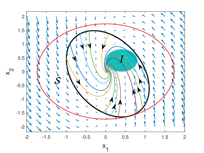
Figure 1 shows the control invariant sets defined by CBF and CBC. The red and light blue disc represent the safe and initial sets, respectively. The interior of the deep blue curve is the invariant set $\mathcal{B}_{2}$ defined by CBF, and the interior of the black curve is the invariant set $\mathcal{B}_{1}$ defined by CBC. It can be seen from the figure that $\mathcal{B}_{1}$ is “larger” than $\mathcal{B}_{2}$. Actually we have $\mathcal{B}_{2}\subset\mathcal{B}_{1}$, which is proved by there exists a SOS multiplier $\sigma$, such that $B_{1}(x)-\sigma B_{2}(x)\in\Sigma[x]$. The reason is that, we trivially have $\sigma_{\mathrm{cbf}}+\alpha\in\mathcal{R}[x]$. A larger search area enables us to find a larger control invariant set. On the other hand, the additional term $\lambda_{1}B_{1}(x)$ can be regarded as an adapted relaxation term compared with a fixed class-$\mathcal{K}$ function used in CBF approach. By using a zeroth order base for the polynomial multiplier $\lambda_{1}$ and expanding the definition domain of CBF to the whole real space, our formulation is equivalent to CBF. Higher order basis selections hereby reduce conservativeness.

Figure 2 shows the value of relaxation coefficient $\lambda_{1}$ and $\alpha$. The multiplier $\lambda_{1}$ includes the following monomial basis: $[x_{1}^{2},x_{1}x_{2},x_{2}^{2},x_{1},x_{2},1]$. It can be seen that $\lambda_{1}$ varies in the control invariant set, which therefore endows the formulation flexibility. An interesting property here is that $\alpha$ cannot be too large, this is because for $x\in\bar{\mathcal{B}_{1}}$, $\alpha B_{2}(x)<0$. In addition, with a non-empty safe set $S\subset\mathbb{R}^{n}$, we directly have $B_{1}(x)\notin\Sigma[x]$, and $\alpha B_{1}(x)\notin\Sigma[x]$.

The control invariant set $\mathcal{B}_{1}$ obtained by CBC design and values of the safe controllers are shown in Figure 3. The vector field, which is represented by the arrows in Figure 3(a) point inside $\mathcal{B}_{1}$ on $\partial{\mathcal{B}_{1}}$. The value of the polynomial control law $u_{(}x)$ is within $[-1.5,1.5]$ in both coordinates.

Consider a second order linear model

where $u_{1}\in[-2.5,2.5]$, $u_{2}\in[-2.5,2.5]$. The system is unstable since the eigenvalues of the state matrix $\begin{bmatrix}2&1\\ 3&1\end{bmatrix}$ are $3.3$ and $-0.3$, whereas it is locally stabilizable. The safe set is defined by a disc $S=\{x|x_{1}^{2}+x_{2}^{2}-3\leq 0\}$. The trajectories of the system start from the following initial set $I=\{x|(x_{1}-0.4)^{2}+(x_{2}-0.4)^{2}-0.16\leq 0\}$. Clearly, all trajectories starting from the initial set tend to infinity, since the system is unstable. Safety is therefore violated with a closed safe region set.

Using a second degree basis $[1,x_{1},x_{2},x_{1}x_{2},x_{1}^{2},x_{2}^{2}]$, a feasible candidate CBC is given by $B_{1}(x)=-7.635x_{1}^{2}-3.439x_{1}x_{2}-3.4024x_{2}^{2}+0.5x_{1}-0.4x_{2}+7.402$. The corresponding control inputs lying inside $[-2.5,2.5]$ when $x\in\partial\mathcal{B}_{1}$ are $u_{1}(x)=-2.32x_{1}-1.11x_{2}+0.022$, $u_{2}(x)=-2.12x_{1}-1.27x_{2}-0.046$. Obviously $u_{1}(x)$ and $u_{2}(x)$ are admissible only within some local regions. More specifically, within $\mathcal{B}_{1}$. We can show the boundary condition $\frac{\partial B_{1}(x)}{\partial x}(f(x)+g(x)u(x))+\lambda_{1}B_{1}(x)-\epsilon_{2}\geq 0$ holds by exploiting the SOS decomposition $\frac{\partial B_{1}(x)}{\partial x}(f(x)+g(x)u(x))+\lambda_{1}B_{1}(x)-\epsilon_{2}=Z(x)^{\top}QZ(x)$, where $Z(x)=[1,x_{1},x_{2},x_{1}x_{2},x_{1}^{2},x_{2}^{2}]^{\top}$ and $Q\succeq 0$.

Figure 4(a) shows the zero level set of the quadratic CBC $B_{1}(x)$. With controller $u_{1}(x)$ and $u_{2}(x)$, vector field in (20) guarantees safety with avoiding the unsafe set. For this case, the system admits an ellipsoidal control invariant set. The level sets of $u_{1}(x)$ and $u_{2}(x)$ are shown in Figure 4(b)-4(c). It can be seen that $u(x)\in\mathcal{U}$ for any $x\in\mathcal{B}_{1}$.

We end this section by a brief comparison between CBF and CBC.

From the point of view of set invariance, the zero-super level set of both CBC and CBF are control invariant. CBC, which is a direct interpretation of control invariance to ensure safety, takes initial conditions into consideration as well - without initial conditions, the CBC formulation is equivalent to CBF. Although the definition of CBF involves the existence of a class-$\mathcal{K}$ function, this, however is a straightforward property that holds for both CBC and CBF.

From the aspect of controller design, the CBF-QP approach relies on a given safe control invariant set, which is free for our approach (7). For the case where the control invariant set is constructed a priori, although the CBF approach endows Lipschitz continuity for the resulting controller, it also introduces unnecessary conservativeness since $\dot{B}_{2}(x)$ is bounded by a fixed additional relaxation term. Although there are existing works propose to tune the relaxation coefficient $\alpha$ online [14], additional computational complexity and necessary cost trade-off are also introduced. Our approach (5), on the other hand, is less restricted with an adapted relaxation coefficient $\lambda_{1}$. For systems with mode switching such as power systems, formulation (5) ensures safety. For continuous controller synthesis, we can also formulate a QP with using $\lambda_{1}B_{1}(x)$ as a relaxation term

we recall here $\lambda_{1}$ is a polynomial of $x$, the argument is dropped for simplicity.

References

- [1] J. Guiochet, M. Machin, and H. Waeselynck, “Safety-critical advanced robots: A survey,” Robotics and Autonomous Systems, vol. 94, pp. 43–52, 2017.
- [2] J. Lygeros, “On reachability and minimum cost optimal control,” Automatica, vol. 40, no. 6, pp. 917–927, 2004.
- [3] K. Margellos and J. Lygeros, “Hamilton–jacobi formulation for reach–avoid differential games,” IEEE Transactions on automatic control, vol. 56, no. 8, pp. 1849–1861, 2011.
- [4] S. Prajna and A. Rantzer, “On the necessity of barrier certificates,” IFAC Proceedings Volumes, vol. 38, no. 1, pp. 526–531, 2005.
- [5] F. Blanchini, “Set invariance in control,” Automatica, vol. 35, no. 11, pp. 1747–1767, 1999.
- [6] S. Prajna, A. Jadbabaie, and G. J. Pappas, “A framework for worst-case and stochastic safety verification using barrier certificates,” IEEE Transactions on Automatic Control, vol. 52, no. 8, pp. 1415–1428, 2007.
- [7] S. Prajna and A. Jadbabaie, “Safety verification of hybrid systems using barrier certificates,” in International Workshop on Hybrid Systems: Computation and Control, pp. 477–492, Springer, 2004.
- [8] A. D. Ames, X. Xu, J. W. Grizzle, and P. Tabuada, “Control barrier function based quadratic programs for safety critical systems,” IEEE Transactions on Automatic Control, vol. 62, no. 8, pp. 3861–3876, 2016.
- [9] M. Vidyasagar, Nonlinear systems analysis. SIAM, 2002.
- [10] R. A. Freeman and J. A. Primbs, “Control lyapunov functions: New ideas from an old source,” in Proceedings of 35th IEEE Conference on Decision and Control, vol. 4, pp. 3926–3931, IEEE, 1996.
- [11] X. Xu, J. W. Grizzle, P. Tabuada, and A. D. Ames, “Correctness guarantees for the composition of lane keeping and adaptive cruise control,” IEEE Transactions on Automation Science and Engineering, vol. 15, no. 3, pp. 1216–1229, 2017.
- [12] S.-C. Hsu, X. Xu, and A. D. Ames, “Control barrier function based quadratic programs with application to bipedal robotic walking,” in 2015 American Control Conference (ACC), pp. 4542–4548, IEEE, 2015.
- [13] Y. Chen, H. Peng, and J. Grizzle, “Obstacle avoidance for low-speed autonomous vehicles with barrier function,” IEEE Transactions on Control Systems Technology, vol. 26, no. 1, pp. 194–206, 2017.
- [14] W. Xiao, C. Belta, and C. G. Cassandras, “Adaptive control barrier functions,” IEEE Transactions on Automatic Control, 2021.
- [15] J. Zeng, B. Zhang, Z. Li, and K. Sreenath, “Safety-critical control using optimal-decay control barrier function with guaranteed point-wise feasibility,” in 2021 American Control Conference (ACC), pp. 3856–3863, IEEE, 2021.
- [16] W. Xiao and C. Belta, “Control barrier functions for systems with high relative degree,” in 2019 IEEE 58th conference on decision and control (CDC), pp. 474–479, IEEE, 2019.
- [17] Y. Chen, M. Jankovic, M. Santillo, and A. D. Ames, “Backup control barrier functions: Formulation and comparative study,” arXiv preprint arXiv:2104.11332, 2021.
- [18] X. Tan, W. S. Cortez, and D. V. Dimarogonas, “High-order barrier functions: Robustness, safety and performance-critical control,” IEEE Transactions on Automatic Control, 2021.
- [19] L. Wang, D. Han, and M. Egerstedt, “Permissive barrier certificates for safe stabilization using sum-of-squares,” in 2018 Annual American Control Conference (ACC), pp. 585–590, IEEE, 2018.
- [20] M. Srinivasan, A. Dabholkar, S. Coogan, and P. A. Vela, “Synthesis of control barrier functions using a supervised machine learning approach,” in 2020 IEEE/RSJ International Conference on Intelligent Robots and Systems (IROS), pp. 7139–7145, IEEE, 2020.
- [21] A. Robey, H. Hu, L. Lindemann, H. Zhang, D. V. Dimarogonas, S. Tu, and N. Matni, “Learning control barrier functions from expert demonstrations,” in 2020 59th IEEE Conference on Decision and Control (CDC), pp. 3717–3724, IEEE, 2020.
- [22] A. Clark, “Verification and synthesis of control barrier functions,” arXiv preprint arXiv:2104.14001, 2021.
- [23] M. Nagumo, “Uber die lage der integralkurven gewokhnlicher di! erentialgleichungen,” Proceedings of the Physico-Mathematical Society of Japan, vol. 24, no. 272, p. 559, 1942.
- [24] T. Cunis and I. Kolmanovsky, “Viability, viscosity, and storage functions in model-predictive control with terminal constraints,” Automatica, vol. 131, p. 109748, 2021.
- [25] S. Prajna, A. Papachristodoulou, and P. A. Parrilo, “Introducing sostools: A general purpose sum of squares programming solver,” in Proceedings of the 41st IEEE Conference on Decision and Control, 2002., vol. 1, pp. 741–746, IEEE, 2002.
- [26] A. Papachristodoulou, J. Anderson, G. Valmorbida, S. Prajna, P. Seiler, and P. A. Parrilo, SOSTOOLS: Sum of squares optimization toolbox for MATLAB. http://arxiv.org/abs/1310.4716, 2013. Available from http://www.eng.ox.ac.uk/control/sostools, http://www.cds.caltech.edu/sostools and http://www.mit.edu/˜parrilo/sostools.
- [27] J. F. Sturm, “Using sedumi 1.02, a MATLAB toolbox for optimization over symmetric cones,” Optimization Methods and Software, vol. 11, no. 1-4, pp. 625–653, 1999.