Theoretical study of the process and the isovector partner of
Abstract
We present a theoretical study of , the isovector partner of , in the process . The weak interaction part proceeds through the charm quark decay process: , while the hadronization part takes place in two mechanisms, differing in how the quarks from the weak decay combines into with a quark-antiquark pair with the vacuum quantum numbers. In addition to the contribution from the tree diagram of the , we have also considered the final-state interactions within the chiral unitary approach to generate the intermediate state , then it decays into the final states . We find that the recent experimental measurements on the and invariant mass distributions can be well reproduced, and the proposed mechanism can provide valuable information on the nature of scalar and its isovector partner .
I Introduction
Though the scalar resonance with is a well established state quoted in the Review of Particle Physics (RPP) ParticleDataGroup:2020ssz, it has attracted a lot of discussions and debates on its structure. The main decay channels of the resonance are and , while the decay branching ratio of the resonance is very small ParticleDataGroup:2020ssz. This indicates that resonance has a large component in its wave function. This is indeed what was found in Ref. Close:2005vf. It has also been suggested as a scalar glueball candidate Gui:2012gx; Janowski:2014ppa; Fariborz:2015dou. Furthermore, the scalar mesons , , and cannot be simultaneously accommodated in the quark model, thus they were widely investigated by different mixing schemes Achasov:1995nh; Amsler:1995tu; Amsler:1995td; Li:2000xy; Li:2000yn; Close:2000yk; Li:2000cj.
On the other hand, the was proposed to be a state dynamically generated from the vector meson-vector meson interactions Geng:2008gx; Geng:2009gb; Du:2018gyn, which remains valid even after the vector meson-pseudoscalar meson and pseudoscalar meson-pseudoscalar meson interactions are included in the coupled channel approach Garcia-Recio:2013uva; Wang:2019niy; Wang:2021jub. Within this picture, the couples mostly to the channel and most properties of can be well reproduced Wang:2021jub; Nagahiro:2008bn; Branz:2009cv; Geng:2010kma; Wang:2011tm; MartinezTorres:2012du; Xie:2014gla; Dai:2015cwa; Dai:2018thd; Molina:2019wjj.
In fact, in Refs. Geng:2008gx; Du:2018gyn, an isospin one partner of the state is also obtained, with its mass around MeV and negative -parity. The also couples mostly to the channel, but the and channels are also important. Very similar conclusions are also found in Ref. Wang:2022pin, where these pseudoscalar-pseudoscalar coupled channels were taken into account, while the obtained mass of of Ref. Wang:2022pin is smaller than those predicted in Refs. Geng:2008gx; Du:2018gyn. The properties of the of Refs. Geng:2008gx; Geng:2009gb; Wang:2022pin are collected in Table 1, where the results of Ref. Wang:2022pin are obtained with a cutoff MeV. Within the ranges of the model parameters of Ref. Du:2018gyn, the mass is predicted in the range of MeV. In addition, one isovector scalar resonance with a mass of 1744 MeV is also predicted within the Regge trajectories Wang:2017pxm.
| Set | ||||
|---|---|---|---|---|
| I (Refs. Geng:2008gx; Geng:2009gb) | ||||
| II (Ref. Wang:2022pin) |
Recently, the BESIII Collaboration has performed an amplitude analysis of the process BESIII:2021anf. It is found that there is an enhancement in the invariant mass spectrum around GeV, which was not seen in the BESIII earlier measurements of BESIII:2020ctr. This indicates the existence of the isospin one partner of the resonance, i.e., . In addition, the state was also observed in the invariant mass spectrum of the decay by the BABAR Collaboration BaBar:2021fkz. The Breit-Wigner mass and width of the state 11 1 It should be stressed that in Ref. BESIII:2021anf BESIII does not distinguish between the and , and denotes the combined state as . are determined as,
| (1) | |||||
| (2) |
by BESIII BESIII:2021anf, and
| (3) | |||||
| (4) |
by BABAR BaBar:2021fkz.
Based on the new measurement of BESIII BESIII:2021anf, Ref. Dai:2021owu has investigated the process , where , firstly happen, then undergo the final state interaction to give rise to the final states . Accordingly, the and resonances are dynamically generated from the final state interaction. The production of and states in the and reactions can be explained Dai:2021owu.
In this work, following Ref. Dai:2021owu, we will revisit the process . In addition to the contributions of the and states from the intermediate process , we will also study the contribution of , which could play a role in the intermediate process . We wish to go beyond the work of Ref. Dai:2021owu and study the whole and invariant mass spectra, where we will focus on the roles played by and to describe the line shapes of and , rather than just the and contributions extracted from the experimental data, which was well described in Ref. Dai:2021owu.
The paper is organized as follows. In Sec. II, we present the theoretical formalism of the decay, and in Sec. III, we show our numerical results and discussions, followed by a short summary in Sec. IV.
II Formalism
The decay can proceed via the -wave final state interaction of the intermediate process, or through the intermediate process of with decay in -wave. In the following, we will present the theoretical formalism of these two mechanisms respectively.
II.1 The mechanism of reaction
As shown in Refs. Dai:2021owu; Molina:2019udw; Wang:2021naf; Duan:2020vye, a way for the to proceed is the following: 1) the charmed quark in turns into a strange quark with a pair by the weak decay shown in Fig. 1; 2) the (Fig. 1(a)) or (Fig. 1(b)) pair, together with the () pair with the vacuum quantum numbers created from vacuum, hadronizes into or , and the other and will hadronize to and , respectively; 3) the final-state interactions of the will lead to dynamical generated , and finally it decays into . According to the topological classification of weak decays in Refs. Chau:1982da; Chau:1987tk the above processes proceed via the so-called internal emission mechanism.


The weak decay processes shown in Figs. 1 (a) and (b) can be formulated as following,
| (5) | |||||
| (6) |
where and are the strength of the production vertices, and contain all the dynamical factors. One can rewrite the two-quark two-antiquark products in the following way
| (7) | |||||
| (8) |
where is the matrix in the flavor space, which is defined as
| (9) |
The elements of matrix can be written in terms of the pseudoscalar () or vector () mesons, which are given by Molina:2019udw; Dai:2021owu; Wang:2021naf.
| (10) |
and
| (11) |
The hadronization processes at the quark level in Eqs. (7) and (8) can be reexpressed at the hadronic level as,
| (12) | |||||
| (13) |
where we have neglected those terms with no contribution to the intermediate state. Using Eqs. (12) and (13), we can rewrite Eqs. (5) and (6) as
| (14) | |||||
| (15) |
To study the decay with dynamically generated from the final-state interaction of , we should sum Eqs. (14) and (15) and produce the combination of and in isospin . With the isospin doublet and Close:1979bt, we obtain,
Thus, we have,
| (16) | |||||
We see that the phases of the above two terms have different signs. If one term is dominant, the other one could be small and can be neglected. In this work, we will focus on the contribution from and ignore the contribution. This seems to be a reasonable choice given the reasonable description of the invariant and mass distributions as shown below.
After the production of the pair, the final-state interaction in -wave between and takes place, in which the is produced, and then it decays to in the final state. 22 2 Note that the parameters and are assumed to be independent of the final-state interactions. In Fig. 2 we show the rescattering diagram for the decay.

With the above formalism, the decay amplitude of the process shown in Fig. 2 can be written as 33 3 We take and , where we have ignored the effect of violation.
| (17) | |||||
where is the invariant mass of the system. We define , which will be determined from the branching fraction Br.
The is the loop function for the pair, which depends on . Since the and have large total decay widths, they should be taken into account. For that purpose, the is not , the loop function of two stable particles of masses and , but convoluted in the masses and with the mass distributions of and vector mesons, which can be done following Refs. Geng:2008gx; Molina:2008jw; Xie:2013ula,
| (18) | |||||
with
| (19) | |||||
| (20) |
and
| (21) | |||||
| (22) |
where the Kllen function . In this work, we take , , MeV and MeV. In addition, the masses, widths and spin-parities of the involved particles are listed in Table 2.
| Particle | Mass (MeV) | Width (MeV) | Spin-parity () |
|---|---|---|---|
| 1968.34 | 1.31 | ||
| 139.5704 | — | ||
| 497.611 | — | ||
| 495.644 | — | ||
| 893.605 | 49.05 | ||
| 891.66 | 50.8 | ||
| 895.55 | 47.3 |
In the dimensional regularization scheme, can be written as Molina:2008jw; Xie:2013ula
| (23) | |||||
with
| (24) |
where is a scale of dimensional regularization, and is the subtraction constant. We take MeV and as in Ref. Geng:2008gx. It is worth mentioning that the only parameter dependent part of is . Any change in is reabsorbed by a change in through , so that the loop function is scale independent. It should be noted that the loop function can be also regularized with the cutoff method as in Refs. Wang:2021jub; Wang:2022pin; Wang:2019niy; Lu:2020ste; Oller:1997ti; Oset:1997it.
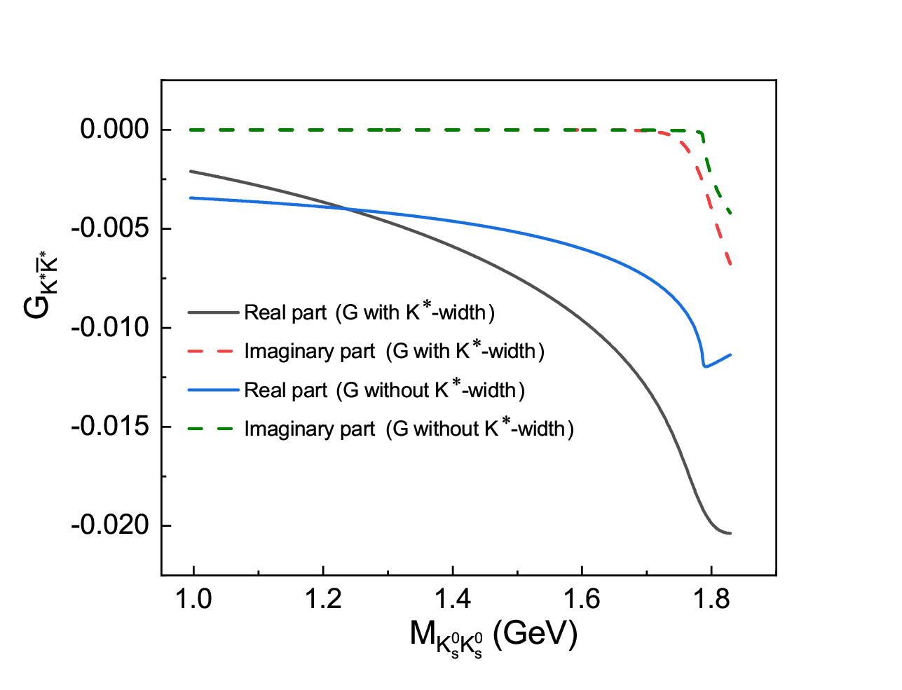
The so obtained real (solid curves) and imaginary (dashed curves) parts of the loop function as a function of the invariant mass are shown in Fig. 3. The results considering the width are obtained with the dimensional regularization method as in Ref. Geng:2008gx, while the results without considering the width are calculated with the cutoff parameter of Ref. Wang:2022pin.
In addition, the in Eq. (17) is the coupling constant of to the channel, and it can be determined from the partial decay width of , which is given by
| (25) |
where is the three momentum of the or meson in the rest frame. With these values of Refs. Geng:2008gx; Geng:2009gb and Ref. Wang:2022pin shown in Table 1, we obtain MeV and MeV for Set I and Set II, respectively. Note that from the partial decay width, one can only obtain the absolute value of the coupling constant, but not the phase. In this work, we assume that is real and positive.
II.2 The mechanism of reaction
In this section, we will present the formalism for the decay via the intermediate meson . According to the RPP ParticleDataGroup:2020ssz, the absolute branching fraction of the decay mode is , which is comparable to the absolute branching fraction of that is . As a result, the is important to produce in the final state through in -wave, as shown in Fig. 4.

The decay amplitude for from the process shown in Fig. 4 can be obtained as
| (26) | |||||
where is the invariant mass squared of the system. The and denote the coupling constants of and , respectively. With the masses of these particles given in Table 2, the branching fraction of Br and the partial decay width quoted in the RPP ParticleDataGroup:2020ssz, we obtain and . Again, we assume that and are real and positive Ling:2021qzl. The uncertainty of originates from the uncertainty of the branching fraction Br, while the uncertainty of is ignored, since it is very small.
II.3 Invariant mass distributions
We can write the total decay amplitude of as follows,
| (27) |
and the double differential width of the decay is
| (28) |
where the interference between and is neglected, since these coupling constants are assumed to be real and positive, as discussed above.
In Ref. BESIII:2021anf, by considering the interference term between and , the extracted branching fraction Br is , which deviates from the CLEO result of Br CLEO:1989zcg. In this work, since the interference term is not included, we use the CLEO result to determine the value of the coupling constant .
Finally, one can easily obtain and , by integrating Eq. (28) over each of the invariant mass variables with the limits of the Dalitz Plot given in the RPP ParticleDataGroup:2020ssz. For example, the upper and lower limits for are as follows:
where the and are the energies of and in the rest frame, respectively,
| (29) |
Similarly, one can obtain the upper and lower limits of .
In Fig. 5 we show the Dalitz Plot of the reaction. The blue band stands for the region in the channel. One can see that the energy region overlaps largely with the state in the channel.

Because the factor is unknown, we determine it from the branching fraction of , which is BESIII:2021anf. With the parameters given in Table 1, we obtain
| (30) |
for Set I, and
| (31) |
for Set II.
III Results and Discussion
In this section, we present the numerical results for the invariant mass distribution of and of the decay. To compare the theoretical invariant mass distributions with the experimental measurements, we introduce an extra global normalization factor , which will be fitted to the experimental data. In Fig. 6, we show our theoretical results for the invariant mass distribution. The red-solid curve stands for the total contributions from the state and the vector meson, while the blue-dashed and green-dot-dashed curves correspond to the contribution from only the and , respectively. The red-solid curve has been adjusted to the strength of the experimental data of BESIII BESIII:2021anf at its peak by taking for both Set I and Set II. One can see that the model results obtained with the parameters of both Set I and Set II can reproduce the experimental data reasonably well, and the plays an important role around the peak of the state. It is clearly seen that the shape of in Fig. 6 (b) is wider than that in Fig. 6 (a). One reason is that, as shown in Table 1, the width of Set II is larger than the one of Set I. The other reason is that the loop function obtained with the cutoff regularization of Ref. Wang:2022pin is smoother than the one of Ref. Geng:2008gx, which can be seen in Fig. 3.


In Ref. Dai:2021owu, the vector-vector intermediate states were produced at the first step with both the external and internal -emission mechanisms, and then the final-state interaction of vector-vector produces and and then they decay into and . By adjusting the effective parameters between these production processes, the ratio of the branching fractions Br and Br from the and contribution can be reproduced Dai:2021owu. Clearly, this work and Ref. Dai:2021owu share the same mechanism for the final-state interactions. As a result, both can describe the main feature of the line shapes. In principle, both the external and internal -emission mechanisms can play a role. However, a quantitative consideration of both mechanisms inevitably introduces additional free parameters for the weak interaction (more details can be found in Ref. Dai:2021owu), which cannot yet be well determined. Hence, we will leave a simultaneous consideration of both mechanisms to a future study when more precise experimental data become available.
It should be noted that the contribution of the state is not considered in our calculation, while the data, on the other hand, contain the contributions of both states. This implies that the peaks of and overlap strongly. Otherwise, the sole contribution from cannot describe the experimental data. The and mixing can also be studied in the decays Molina:2019wjj when more experimental data are available, just as the and mixing BESIII:2018ozj; Wu:2008hx; Wu:2007jh for the case of molecules. In fact, the and mixing was investigated in the decay in Ref. Achasov:2017edm with the formalism built in a earlier work of Ref. Achasov:1979xc, where the mixing of and resonances that breaks the isospin invariance due to the and meson mass difference.
In our model, the final pair is produced from the interaction, and the loop function is very small around the [] pole region (see Fig. 3) and the coupling of [] to the channel Garcia-Recio:2013uva is also small compared with the one of to the channel. Hence, there are no and signal in the mass spectrum of the decay. On the other hand, from Eq. (16), we find that the two phases in the and productions have an opposite sign. If the production of is constructive as shown in the new BESIII data BESIII:2021anf, one can expect no contribution from the mechanism shown in Fig. 1 to produce the resonance in the decay BESIII:2020ctr; Duan:2020vye; Wang:2021ews. However, the could be produced via the external emission mechanism, and its signal is expected in the process .
Next, we turn to the invariant mass distributions. In Fig. 7 we show the theoretical results for the invariant mass distributions of the decay. To compare with the experimental results, we have multiplied a factor of two to , since the experimental distribution of contains two entries of events, one for each (see more details in Ref. BESIII:2021anf). The peak of the can be well described. The contribution from is very small to the peak, while its contribution to the threshold enhancement of the invariant mass distribution is significant.


In addition, with the model parameters as obtained above for the decay, we study the process of , where the contributions from and are taken into account by assuming that the mechanism of is the same as the one of the process of . The numerical results for the and invariant mass distributions are shown in Figs. 8 and 9, respectively. The experimental data are taken from Ref. BESIII:2020ctr. If the plays the dominant role for the structure around GeV2, the invariant mass distribution in the low energy region can not be well described because of the reflection effect of . In Fig. 8, the contribution is scaled by a factor of 4.3, as shown by the pink-dash-dashed curve, and one can see that the contribution is already enough to reasonably describe both the and invariant mass distributions in the energy region considered. which is also consistent with the Dalitz Plot of , as shown in Fig. 6 of Ref. BESIII:2020ctr.
As discussed above, to describe well both and reactions, one needs to consider other mechanisms, especially the contribution from . In this case, we will have more free parameters, and we need more constraints from both theoretical and experimental sides. In the present work, we focus on the role played by the in the decay, and it is found that the new measurements of the reaction can be well reproduced, and the contribution of the around the peak is important.


Finally, it is interesting to note that one can study the state in the channel of the decay by including the contribution of the final-state interaction of , which can be easily obtained by summing the second term of Eqs. (12) and (13). If the very small mass difference of charged and neutral meson is neglected, it is expected that the branching fraction of should be the same as the one of , and hence a charged will be visible in the invariant mass spectrum. Indeed, the was recently observed in the decay of by the BESIII Collaboration BESIII:2022wkv.
IV Summary
In summary, we have studied the Cabibbo-favored process of . By considering the decay mechanism of internal emission, and hadronization of the or with with the vacuum quantum numbers, we obtain in the first step, then the transition of proceeds following final-state interactions of the pair in the chiral unitary approach where the state is dynamically generated. In addition, the tree diagram of is also taken into account.
We have calculated the and invariant mass distributions, which are in good agreement with the experimental measurements of BESIII BESIII:2021anf. We have found that the plays an important role in the peak region. Our study shows that the BESIII measurements support the molecular nature of the and states and they overlap strongly in the data.
For the reproduction of the peak, it is found that the contributions from both the tree diagram as shown in Fig. 4 and the final-state interaction as shown in Fig. 2 are crucial. In addition, within the proposed mechanism, it is expected that the charged signal can show up in the invariant mass distribution of the decay, which should be checked by future experimental measurements.
Acknowledgments
We would like to thank Prof. Eulogio Oset and Prof. Lian-Rong Dai for their careful reading of the manuscript and useful discussions. This work is partly supported by the National Natural Science Foundation of China under Grants Nos. 12075288, 11735003, 11975041, 11961141004, 11961141012, and 12192263. This work is supported by the Natural Science Foundation of Henan under Grand No. 222300420554, the Key Research Projects of Henan Higher Education Institutions under No. 20A140027, the Project of Youth Backbone Teachers of Colleges and Universities of Henan Province (2020GGJS017), the Youth Talent Support Project of Henan (2021HYTP002), the Fundamental Research Cultivation Fund for Young Teachers of Zhengzhou University (JC202041042), and the Open Project of Guangxi Key Laboratory of Nuclear Physics and Nuclear Technology, No. NLK2021-08.
References
- (1) P. A. Zyla et al. [Particle Data Group], PTEP 2020, 083C01 (2020).
- (2) F. E. Close and Q. Zhao, Phys. Rev. D 71, 094022 (2005).
- (3) L. C. Gui et al. [CLQCD], Phys. Rev. Lett. 110, 021601 (2013).
- (4) S. Janowski, F. Giacosa and D. H. Rischke, Phys. Rev. D 90, 114005 (2014).
- (5) A. H. Fariborz, A. Azizi and A. Asrar, Phys. Rev. D 92, 113003 (2015).
- (6) N. N. Achasov and G. N. Shestakov, Phys. Rev. D 53, 3559-3563 (1996).
- (7) C. Amsler and F. E. Close, Phys. Lett. B 353, 385-390 (1995).
- (8) C. Amsler and F. E. Close, Phys. Rev. D 53, 295-311 (1996).
- (9) D. M. Li, H. Yu and Q. X. Shen, Mod. Phys. Lett. A 15, 1781-1788 (2000).
- (10) D. M. Li, H. Yu and Q. X. Shen, Commun. Theor. Phys. 34, 507-512 (2000).
- (11) F. E. Close and A. Kirk, Phys. Lett. B 483, 345-352 (2000).
- (12) D. M. Li, H. Yu and Q. X. Shen, Eur. Phys. J. C 19, 529-533 (2001).
- (13) L. S. Geng and E. Oset, Phys. Rev. D 79, 074009 (2009).
- (14) M. L. Du, D. Gülmez, F. K. Guo, U. G. Meißner and Q. Wang, Eur. Phys. J. C 78, 988 (2018).
- (15) L. S. Geng, E. Oset, R. Molina and D. Nicmorus, PoS EFT09, 040 (2009).
- (16) C. García-Recio, L. S. Geng, J. Nieves, L. L. Salcedo, E. Wang and J. J. Xie, Phys. Rev. D 87 (2013) no.9, 096006
- (17) Z. L. Wang and B. S. Zou, Phys. Rev. D 99, 096014 (2019).
- (18) Z. L. Wang and B. S. Zou, Phys. Rev. D 104, 114001 (2021).
- (19) H. Nagahiro, L. Roca, E. Oset and B. S. Zou, Phys. Rev. D 78, 014012 (2008).
- (20) R. Molina, L. R. Dai, L. S. Geng and E. Oset, Eur. Phys. J. A 56, 173 (2020).
- (21) T. Branz, L. S. Geng and E. Oset, Phys. Rev. D 81, 054037 (2010).
- (22) L. S. Geng, F. K. Guo, C. Hanhart, R. Molina, E. Oset and B. S. Zou, Eur. Phys. J. A 44, 305-311 (2010).
- (23) W. L. Wang and Z. Y. Zhang, Phys. Rev. C 84, 054006 (2011).
- (24) A. Martinez Torres, K. P. Khemchandani, F. S. Navarra, M. Nielsen and E. Oset, Phys. Lett. B 719, 388-393 (2013).
- (25) J. J. Xie and E. Oset, Phys. Rev. D 90, 094006 (2014).
- (26) L. R. Dai, J. J. Xie and E. Oset, Phys. Rev. D 91, 094013 (2015).
- (27) L. R. Dai, R. Pavao, S. Sakai and E. Oset, Eur. Phys. J. A 55, 20 (2019).
- (28) Z. L. Wang and B. S. Zou, Eur. Phys. J. C 82 (2022) no.6, 509
- (29) G. Y. Wang, S. C. Xue, G. N. Li, E. Wang and D. M. Li, Phys. Rev. D 97 (2018) no.3, 034030
- (30) M. Ablikim et al. [BESIII], Phys. Rev. D 105, L051103 (2022).
- (31) J. P. Lees et al. [BaBar], Phys. Rev. D 104, 072002 (2021).
- (32) L. R. Dai, E. Oset and L. S. Geng, Eur. Phys. J. C 82, 225 (2022).
- (33) R. Molina, J. J. Xie, W. H. Liang, L. S. Geng and E. Oset, Phys. Lett. B 803, 135279 (2020).
- (34) J. Y. Wang, M. Y. Duan, G. Y. Wang, D. M. Li, L. J. Liu and E. Wang, Phys. Lett. B 821, 136617 (2021).
- (35) M. Y. Duan, J. Y. Wang, G. Y. Wang, E. Wang and D. M. Li, Eur. Phys. J. C 80, 1041 (2020).
- (36) L. L. Chau, Phys. Rept. 95, 1-94 (1983).
- (37) L. L. Chau and H. Y. Cheng, Phys. Rev. D 36, 137 (1987); Phys. Rev. D 39, 2788 (1989) (addendum).
- (38) F. E. Close, An Introduction to Quarks and Partons, Academic Press, London 1979, 481 pp
- (39) R. Molina, D. Nicmorus and E. Oset, Phys. Rev. D 78, 114018 (2008).
- (40) J. J. Xie, M. Albaladejo and E. Oset, Phys. Lett. B 728, 319-322 (2014).
- (41) J. X. Lu, C. H. Zeng, E. Wang, J. J. Xie and L. S. Geng, Eur. Phys. J. C 80, 361 (2020).
- (42) J. A. Oller and E. Oset, Nucl. Phys. A 620, 438-456 (1997) [erratum: Nucl. Phys. A 652, 407-409 (1999)].
- (43) E. Oset and A. Ramos, Nucl. Phys. A 635, 99-120 (1998).
- (44) X. Z. Ling, M. Z. Liu, J. X. Lu, L. S. Geng and J. J. Xie, Phys. Rev. D 103, 116016 (2021).
- (45) W. Y. Chen et al. [CLEO], Phys. Lett. B 226, 192-196 (1989).
- (46) M. Ablikim et al. [BESIII], Phys. Rev. Lett. 121, 022001 (2018).
- (47) J. J. Wu and B. S. Zou, Phys. Rev. D 78, 074017 (2008).
- (48) J. J. Wu, Q. Zhao and B. S. Zou, Phys. Rev. D 75, 114012 (2007).
- (49) N. N. Achasov and G. N. Shestakov, Phys. Rev. D 96, 036013 (2017).
- (50) N. N. Achasov, S. A. Devyanin and G. N. Shestakov, Phys. Lett. B 88, 367-371 (1979).
- (51) M. Ablikim et al. [BESIII], Phys. Rev. D 104, 012016 (2021).
- (52) Z. Y. Wang, J. Y. Yi, Z. F. Sun and C. W. Xiao, Phys. Rev. D 105, 016025 (2022).
- (53) M. Ablikim et al. [BESIII], [arXiv:2204.09614 [hep-ex]].