reception date \Acceptedacception date \Publishedpublication date
atomic processes — ISM: supernova remnants — X-rays: individual (SNR J0453.66829) — X-rays: ISM
High resolution X-ray study of supernova remnant J0453.66829 with unusually high forbidden-to-resonance ratio
Abstract
Recent high-resolution X-ray spectroscopy has revealed that several supernova remnants (SNRs) in the Large Magellanic Cloud (LMC) show unusually high forbidden-to-resonance () line ratios. While their origin is still uncertain and debated, most of these SNRs have asymmetric morphology and/or show evidence of interaction with dense material, which may hint at the true nature of the anomalous ratios. Here we report on a detailed spectral analysis of an LMC SNR J0453.66829 with the Reflection Grating Spectrometer (RGS) onboard XMM-Newton. We find that the ratio of O () is significantly higher than expected from the previously-reported thermal model. The spectrum is fairly explained by taking into account a charge exchange (CX) emission in addition to the thermal component. Analyzing archival ATCA & Parkes radio data, we also reveal that H\emissiontypeI cloud is possibly interacting with J0453.66829. These results support the presence of CX in J0453.66829, as the origin of the obtained high ratio. Although a contribution of the resonance scattering (RS) cannot be ruled out at this time, we conclude that CX seems more likely than RS considering the relatively symmetric morphology of this remnant.
1 Introduction
Plasma diagnostics of astrophysical objects using line ratios of He-like ions (Gabriel & Jordan 1969, i.e., and ratios; ) will become a part of mainstream in the upcoming era of high-resolution X-ray spectroscopy. Recent grating observations revealed that several supernova remnants (SNRs) have anomalous line ratios of O, in which the forbidden line intensity relative to the resonance line (hereafter, ) is significantly higher than expected for an ordinary thermal plasma (Katsuda et al. 2011; Uchida et al. 2019, e.g.,). While their physical origin is still under debate, two interpretations have mainly been argued: charge exchange (CX) and resonance scattering (RS), both of which were predicted to occur in SNRs by previous calculations (Lallement 2004; Kaastra & Mewe 1995, e.g.,). The presence of the CX emission and/or RS effect would hinder accurate plasma diagnostics, and, more importantly, these physical processes themselves work as useful probes to obtain key information such as collision and turbulent velocities. It is therefore required to know physical conditions and surrounding environments in which CX and/or RS can occur, that is, to reveal the origin of the anomalously high ratios of O found in SNRs.
On the basis of observations with the Reflection Grating Spectrometer (RGS) onboard XMM-Newton, previous analyses of SNRs in the Large Magellanic Cloud (LMC) indicate that several of them tend to have relatively high ratios of O; N23 (Broersen et al. 2011), N49 (Amano et al. 2020), and N132D (Suzuki et al. 2020). They are located in a dense ambient medium as suggested by radio-line (Banas et al. 1997; Sano et al. 2017, e.g.,) or infrared observations (Williams et al. 2006, e.g.,), which may hint at the cause of the anomalous spectral features. In this context, we found that no detailed spectroscopy has been performed so far for the middle-aged LMC SNR J0453.66829, although this remnant is in a dense environment similar to N23 and N132D according to Williams et al. 2006.
J0453.66829 is a relatively compact ( in diameter) remnant of a core-collapse explosion (Lopez et al. 2009; McEntaffer et al. 2012), containing a pulsar wind nebula (PWN) at the center of the shell (Gaensler et al. 2003). In addition to synchrotron radiation from the PWN, McEntaffer et al. 2012 indicated that the X-ray spectrum of J0453.66829 obtained with Chandra is well explained by a shock-heated interstellar medium (ISM). A similar conclusion was reached by Haberl et al. 2012, who performed multi-frequency observations of J0453.66829, including X-ray band with XMM-Newton. In their spectral fit, the forbidden line of O is seemingly higher than a normally expected thermal model. In this paper, we thus revisit the RGS data with particular attention to the He-like lines, in conjunction with an H observation around the remnant, in order to investigate the relation between the ratio and surrounding environment of J0453.66829. Errors are given at the 68% confidence level throughout the paper. We assume the distance to J0453.66829 to be 50 kpc (Pietrzyński et al. 2013).
2 Observation and data reduction

J0453.66829 was observed with XMM-Newton on 2001 March 29 (Obs. IDs 0062340101 and 0062340501). Since one of the data sets (Obs. ID 0062340501) was affected by large soft-proton flares, we present results only from Obs. ID 0062340101. The raw data were processed with the XMM Science Analysis Software (SAS) version 18.0.0 and the calibration data files released in 2020 June. In the following spectral analysis, we combine RGS1 and RGS2 data with MOS spectra. After discarding periods of background flares, we obtained MOS and RGS data with effective exposure times of ks and ks, respectively. We do not analyze second order spectra because of their poor statistics.
3 Analysis and results
Figure 1 shows a background-subtracted true-color image of J0453.66829 taken by EPIC (MOS and pn). We extracted RGS spectra by limiting the cross-dispersion width so as to cover the whole of J0453.66829. MOS spectra were obtained from the entire region of the remnant. Off-source regions in the field of view (FOV) were used to extract background spectra for each instrument. We simultaneously fitted the unbinned RGS and MOS spectra using SPEX version 3.06.01 (Kaastra et al. 1996), applying a maximum likelihood method, W-stat (Wachter et al. 1979). Throughout this analysis, the hydrogen column density () of the Galactic absorption was fixed to cm-2 (Dickey & Lockman 1990) and that of the LMC was left free. We referred to Russell & Dopita 1992 for the elemental abundances of the LMC.


Figure 2 presents the MOS and RGS spectra of J0453.66829. McEntaffer et al. 2012 reported that the X-ray spectrum of J0453.66829 can be explained by a two-temperature non-equilibrium ionization (NEI) model (neij) with a power-law component for the PWN. We first applied this “2-NEI” model, in which photon index and normalization of the power-law component were fixed to 2.0 and (McEntaffer et al. 2012), respectively. Free parameters for the thermal components include the electron temperature (), ionization timescale (, where and are the electron number density and the time after shock heating, respectively), and emission measure (, where is the emitting volume of the plasma). Abundances of C, N, O, Ne, Mg, Si, and Fe were set free and tied between the two components.
The best-fit model of the 2-NEI model is plotted in Figure 2, and its parameters are summarized in Table 3. We found that whereas the model can reproduce the MOS spectrum, significant residuals remain in the RGS spectrum especially at the O He and O Ly lines. The result implies that some additional considerations are required to better explain the fine structures of the spectrum of J0453.66829. To clarify this point, we quantified the intensity ratio of O by adding four Gaussians instead of multiplet line components of O He, (i.e., resonance, forbidden and intercombination lines) implemented in the neij code: in this method, the other lines and continua were not changed and were the same as those of the best-fit model. We compared the obtained value with that expected from the NEI model as indicated in Figure 3 (a). The resultant ratio, requires keV. On the other hand, few O6+ (He like) ions, which emit O, are present in such a low-temperature plasma (panel (b) of Figure 3), being inconsistent with our result. We thus conclude that any single or multiple NEI component(s) cannot reproduce the observed RGS spectrum. Another possible scenario to account for both ratio and O Ly line is an over-ionized plasma. This scenario, however, would make a significant excess of radiative recombination continua, and thus contradicts the observed spectrum.
Best-fit parameters of the J0453.66829 spectrum Component Parameters (unit) 2-NEI 2-NEICX 2-NEIGaus (RS) Absorption (1020 cm-2) (fixed) (fixed) (fixed) (1020 cm-2) Power law (PWN) Normalization () (fixed) (fixed) (fixed) (fixed) (fixed) (fixed) Low-temperature NEI Emission Measure () (keV) C N O Ne Mg Si Fe High-temperature NEI Emission Measure () (keV) CX Emission Measure () Negative Gaussian ∗ ∗* ∗ ∗*footnotemark: : Ne He () Normalization () Fe L(3d-2p) Normalization () Fe L(3s-2p) Normalization () O Ly Normalization () O He () Normalization () W-statistic/d.o.f. 4124/3627 4107/3625 4085/3622 {tabnote} ∗ ∗* ∗ ∗*footnotemark: The line centroid wavelengths of the Gaussians at Ne He (), Fe L(3d-2p), Fe L(3s-2p), O Ly, and O He () are fixed to 13.4 Å, 15.0 Å, 17.0 Å, 18.9 Å, and 21.6 Å, respectively.
We next added a CX component to the 2-NEI model (hereafter, 2-NEICX model) to enhance the forbidden line intensity of O, as Uchida et al. 2019 did for a similar case of the Cygnus Loop. Free parameters of the CX model are normalization (, where is the density of the neutral materials) and shock velocity (). The ionization temperature was tied to of the low-temperature NEI component. The best-fit result and parameters are shown in Figure 4 and Table 3, respectively. As a result, we successfully fitted the RGS spectrum with the 2-NEICX model, except that the discrepancy between the data and model is still seen at the O Ly line.
A similar excess of the O Ly line has been reported by Amano et al. 2020, who analyzed the RGS spectrum of N49 and concluded that the line ratios including of O can be reasonably explained by taking into account the effect of RS. We thus applied negative Gaussians in addition to the 2-NEI model (hereafter, 2-NEIGaus model), in which we assumed that the SNR shell is a slab and all scattered photons will escape from the line of sight (Kaastra & Mewe 1995). The Gaussians were fixed at the centroid wavelengths of the lines whose oscillator strengths are relatively large: resonance lines of Ne and O, Fe L(3d-2p), Fe L(3s-2p), and O Ly. Normalizations (photons ) of these five Gaussians were set free and the other parameters are the same as the 2-NEI model. As shown in Figure 4, the 2-NEIGaus model globally reduces the residuals. The best-fit parameters (Table 3) are consistent with those expected for a typical middle-aged SNR. We therefore claim that a presence of RS cannot be ruled out in terms of the spectral fitting.

4 Discussion
As indicated in the previous section, the high-resolution X-ray spectrum of J0453.66829 suggests the presence of CX or RS in the remnant. Similar cases have often been discussed in the literature (Uchida et al. 2019; Amano et al. 2020; Suzuki et al. 2020, e.g.,). Although it is in general difficult to distinguish between these two possibilities with the available spectroscopies, the SNR morphology and surrounding environment may provide a clue to the true origin of the high ratio. In Table 4.1, we summarize LMC/SMC SNRs for which the (or ) ratios were measured so far using the RGS to compare our results with those from other SNRs in the discussion below.

4.1 X-ray Morphology of J0453.66829
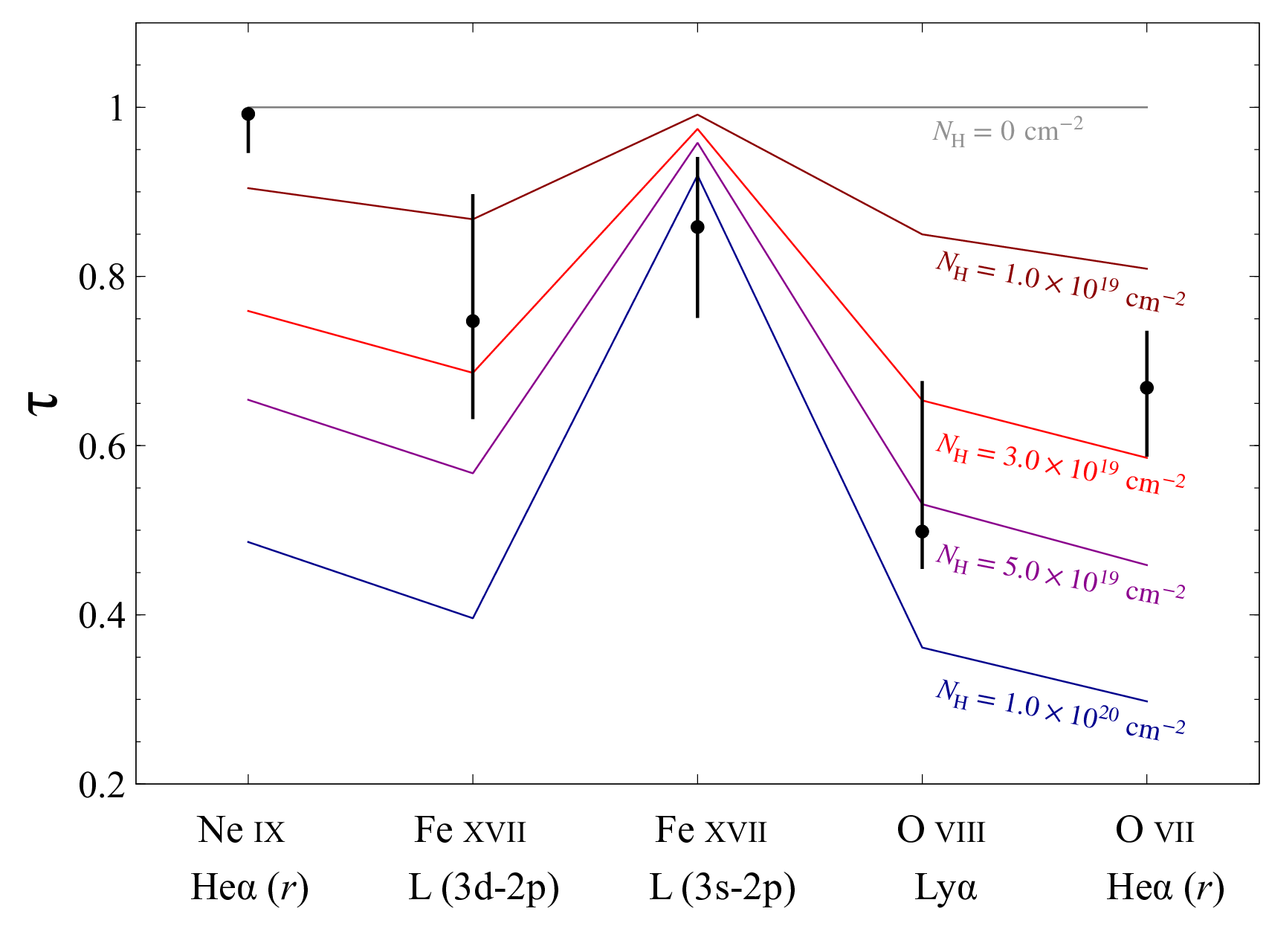
For quantitative evaluation of the effect of RS, we calculated a transmission factor by applying the same method as Amano et al. 2020. We compared theoretical values of for several optical depths according to Kaastra & Mewe 1995 with those estimated from the best-fit normalizations of the negative Gaussians. Figure 5 shows the result. Although the model fails to explain the observed resonance line of Ne, the estimated for J0453.66829 are roughly consistent with those at – cm-2, which corresponds to a plasma depth of 3–18 pc under an assumption of the plasma density cm-3 (Williams et al. 2006). Since the diameter of J0453.66829 is estimated to be pc from the apparent angular size of the shell (), the line-of-sight plasma depth that contributes to RS should be 10–50% of the diameter. If this is really the case, the shell-type SNR would be required to have a highly asymmetric morphology; for instance, a bright shell is prominent only on one side of the remnant (see Figure 6).
If J0453.66829 has an ideal spherical symmetric structure, the RS effect will be cancelled out and an enhancement of will not occur. Note that the RGS spectrum of J0453.66829 was obtained from the entire region. We can thus postulate that asymmetry of an SNR is a key parameter to evaluate the effect of RS. From a soft-band imaging analysis by Lopez et al. 2011, we found that J0453.66829 has a less asymmetric morphology among the six SNRs listed in Table 4.1. Other core-collapse remnants are more “elliptical” (N23) or “non-uniform” (N132D), which are parametrized as and in their calculation. Although N49 was not analyzed by Lopez et al. 2011, it would also be categorized as a highly elliptical remnant due to its morphology similar to that of N23. It is reasonable that N23, N49, and N132D show relatively high ratios due to RS, as claimed by previous studies (Broersen et al. 2011; Amano et al. 2020; Suzuki et al. 2020). On the other hand, in the case of J0453.66829, the effect of RS might be unlikely or insufficient to satisfactorily explain the observed high ratio.
ratios or -ratios for O He
Name
Type of SNe
Ref.
Age
Ref.
f/r or G ratios
Ref.
Surrounding
Ref. Surrounding
Type
∗
∗*
∗
∗*footnotemark:
(yr)
Age
∗
∗*
∗
∗*footnotemark:
Ratios
∗
∗*
∗
∗*footnotemark:
environments
environments
∗
∗*
∗
∗*footnotemark:
1E 01027219
Ib/c or IIL/b
1, 2
1000
3
‡
‡{\ddagger}
‡
‡{\ddagger}footnotemark:
4
no data
N132D
Ib
1
2500
5
†
†{\dagger}
†
†{\dagger}footnotemark:
6
CO and H\emissiontypeI clouds
7, 8, 9
DEM L71
Ia
10
4400
11
†
†{\dagger}
†
†{\dagger}footnotemark:
12
no data
N23 (050668.0)
II
13
4600
13
‡
‡{\ddagger}
‡
‡{\ddagger}footnotemark:
14
star-forming region
15
N49
II
16
6600
17
‡
‡{\ddagger}
‡
‡{\ddagger}footnotemark:
18
CO and H\emissiontypeI clouds
7, 8, 19
J0453.66829
II
20
13000
21
†
†{\dagger}
†
†{\dagger}footnotemark:
22
H\emissiontypeI clouds
22
{tabnote}
∗
∗*
∗
∗*footnotemark:
References.
(1) Blair et al. 2000;
(2) Chevalier 2005;
(3) Hughes et al. 2000;
(4) Rasmussen et al. 2001;
(5) Vogt & Dopita 2011;
(6) Suzuki et al. 2020;
(7) Banas et al. 1997;
(8) Sano et al. 2017;
(9) Sano et al. 2020;
(10) Hughes et al. 1998;
(11) Ghavamian et al. 2003;
(12) van der Heyden et al. 2003;
(13) Hughes et al. 2006;
(14) Broersen et al. 2011;
(15) Chu & Kennicutt 1988;
(16) Uchida et al. 2015;
(17) Park et al. 2003;
(18) Amano et al. 2020;
(19) Yamane et al. 2018;
(20) Lopez et al. 2009;
(21) Gaensler et al. 2003;
(22) This work.
†
†{\dagger}
†
†{\dagger}footnotemark:
ratio
‡
‡{\ddagger}
‡
‡{\ddagger}footnotemark:
ratio
4.2 Surrounding Environment of J0453.66829


CX is another possibility that causes the enhancement of . An interaction with a dense ambient medium is expected in this case, as in previous studies of Galactic SNRs with the RGS: Puppis A (Katsuda et al. 2012) and the Cygnus Loop (Uchida et al. 2019). While McEntaffer et al. 2012 implied a presence of dense gas in the vicinity of J0453.66829 because of a spatial correlation between the X-ray and infrared morphologies, the surrounding environment of this remnant has still been unclear (Williams et al. 2006; Lakićević et al. 2015). As shown in Figure 7, we compared the ATCA & Parkes (Kim et al. 2003) H\emissiontypeI velocity channnel map around J0453.66829 with the X-ray morphology and found H\emissiontypeI clouds located along with the southwestern half of J0453.66829. Figure 8 shows the integrated intensity maps of H\emissiontypeI. We also found the southwestern part of the remnant is increasingly covered with an H\emissiontypeI cloud. The position-velocity diagram suggests that the SNR shell is expanding into the dense gas (panel (b) of Figure 8).


If the SNR shell interacts with the H\emissiontypeI cloud in the southwestern region, relatively strong forbidden line emission would be detected there. We thus divided the data into two in the cross-dispersion direction (namely, northeast; NE and southwest; SW) as indicated in Figure 1. As displayed in Figure 9, the forbidden line intensity of O in SW is stronger than that in NE. Applying the same method as the entire region, we obtained ratios of and for NE and SW, respectively. Although statistically they are equal within the errors, the trend is consistent with the above expectation and thus strongly supports the presence of CX. The best-fit models of 2-NEICX for these regions are displayed in Figure 10. The model parameters are given in Table 5. While the CX component is required both in NE and SW, its contribution is relatively dominant in SW. We thus confirmed that the anomalous ratios is due to the CX emission, mainly caused by an interaction with the southwestern H\emissiontypeI cloud.
According to the discussion above, we presume that the emitting region of CX is the southwestern edge of J0453.66829, which is in contact with the H\emissiontypeI cloud. To quantitatively examine the possibility of CX, we estimate the emitting volume using the volume emission measure of the CX component , where is the neutral material density of the surrounding gas. Given that the H\emissiontypeI gas has a typical density of cm-3, we obtain the emitting volume to be cm3. Since the total volume of J0453.66829 is estimated to be cm3 assuming a diameter of pc, we conclude that the CX occurs in of the SNR radius. The result fits well with the calculation by Lallement 2004 and thus supports the possibility that the observed anomalous ratio is due to CX. Note that the significant residuals seen at 16 Å (section 3) is still an open question; such discrepancies around the O Ly line are often pointed out by many RGS observations (Amano et al. 2020, e.g.,), and might be due to uncertainties in the atomic data (de Plaa et al. 2012, see also,).
5 Conclusions
We performed a high-resolution spectroscopy of J0453.66829 with the RGS onboard XMM-Newton and found that the intensity of the forbidden line of O is significantly stronger than expected from a simple thermal (2-NEI) model. To account for the obtained high ratio (), we examined two possibilities: CX and RS, which have been proposed for explaining similar spectral features found in SNRs. Both models are statistically acceptable, although small residuals remain at 16 Å (around the O Ly line) between the data and the 2-NEICX model. Such discrepancies are often pointed out by many RGS observations (de Plaa et al. 2012; Amano et al. 2020, e.g.,) and are likely due to uncertainties in the atomic data. From the best-fit result with the RS model, we estimated a transmission factor ; the result requires a significantly asymmetric shape along the line of sight. This may be inconsistent with the apparent morphology of J0453.66829, since a previous systematic X-ray study indicates that this remnant is one of the “least asymmetric” core-collapse SNRs (Lopez et al. 2011). On the other hand, our estimate of the emitting volume for the CX component ( of the SNR radius) agrees well with a theoretical expectation (Lallement 2004). We also found evidence of an interaction between J0453.66829 and the dense ambient gas in the ATCA & Parkes H\emissiontypeI map, which supports the picture that the observed ratio is due to the CX emission at SNR shock fronts. In conclusion, the presence of CX in J0453.66829 is favored in our study, while a slight or significant contribution of the RS effect also cannot be ruled out. Future spatially resolved spectroscopies with high angular resolution missions like Athena will clarify this point.
Best-fit parameters of the NE and SW spectra Component Parameters (unit) 2-NEICX NE SW Absorption (1020 cm-2) (fixed) (1020 cm-2) Power law (PWN) Normalization () (fixed) (fixed) Low-temperature NEI Emission Measure () (keV) C N O Ne Mg Si Fe High-temperature NEI Emission Measure () (keV) CX Emission Measure () W-statistic/d.o.f. 4108/3625 4107/3625
We thank Brian J. Williams for a helpful discussion about the previous multiwavelength studies of the SNR J0453.66829. The ATCA and the Parkes radio telescope are all part of the Australia Telescope National Facility, which is funded by the Australian Government for operation as a National Facility managed by CSIRO. We acknowledge the Gomeroi and Wiradjuri people as the traditional owners of the Observatory sites. This work is supported by JSPS/MEXT KAKENHI Scientific Research Grant Numbers JP19K03915 (H.U.), JP19H01936 (T.T.), JP19K14758 (H.S.), JP20KK0309 (H.S.), and JP21H04493 (T.G.T. and T.T.).
References
- Amano et al. (2020) Amano, Y., Uchida, H., Tanaka, T., et al. 2020, ApJ, 897, 12.
- Banas et al. (1997) Banas, K. R., Hughes, J. P., Bronfman, L., et al. 1997, ApJ, 480, 607.
- Bhardwaj et al. (2007) Bhardwaj, A., Elsner, R. F., Randall Gladstone, G., et al. 2007, Planet. Space Sci., 55, 1135.
- Blair et al. (2000) Blair, W. P., Morse, J. A., Raymond, J. C., et al. 2000, ApJ, 537, 667.
- Broersen et al. (2011) Broersen, S., Vink, J., Kaastra, J., et al. 2011, A&A, 535, A11.
- Chevalier (2005) Chevalier, R. A. 2005, ApJ, 619, 839.
- Chu & Kennicutt (1988) Chu, Y.-H. & Kennicutt, R. C. 1988, AJ, 96, 1874.
- Cravens (2002) Cravens, T. E. 2002, Science, 296, 1042.
- de Plaa et al. (2012) de Plaa, J., Zhuravleva, I., Werner, N., et al. 2012, A&A, 539, A34.
- Dickey & Lockman (1990) Dickey, J. M. & Lockman, F. J. 1990, ARA&A, 28, 215.
- Gabriel & Jordan (1969) Gabriel, A. H. & Jordan, C. 1969, MNRAS, 145, 241.
- Gaensler et al. (2003) Gaensler, B. M., Hendrick, S. P., Reynolds, S. P., et al. 2003, ApJ, 594, L111.
- Ghavamian et al. (2003) Ghavamian, P., Rakowski, C. E., Hughes, J. P., et al. 2003, ApJ, 590, 833.
- Haberl et al. (2012) Haberl, F., Filipović, M. D., Bozzetto, L. M., et al. 2012, A&A, 543, A154.
- Hester & Cox (1986) Hester, J. J. & Cox, D. P. 1986, ApJ, 300, 675.
- Hitomi Collaboration et al. (2018) Hitomi Collaboration, Aharonian, F., Akamatsu, H., et al. 2018, PASJ, 70, 10.
- Hughes et al. (1998) Hughes, J. P., Hayashi, I., & Koyama, K. 1998, ApJ, 505, 732.
- Hughes et al. (2000) Hughes, J. P., Rakowski, C. E., & Decourchelle, A. 2000, ApJ, 543, L61.
- Hughes et al. (2006) Hughes, J. P., Rafelski, M., Warren, J. S., et al. 2006, ApJ, 645, L117.
- Kaastra & Mewe (1995) Kaastra, J. S. & Mewe, R. 1995, A&A, 302, L13
- Kaastra et al. (1996) Kaastra, J. S., Mewe, R., & Nieuwenhuijzen, H. 1996, UV and X-ray Spectroscopy of Astrophysical and Laboratory Plasmas, 411
- Katsuda et al. (2011) Katsuda, S., Tsunemi, H., Mori, K., et al. 2011, ApJ, 730, 24.
- Katsuda et al. (2012) Katsuda, S., Tsunemi, H., Mori, K., et al. 2012, ApJ, 756, 49.
- Kim et al. (2003) Kim, S., Staveley-Smith, L., Dopita, M. A., et al. 2003, ApJS, 148, 473.
- Lakićević et al. (2015) Lakićević, M., van Loon, J. T., Meixner, M., et al. 2015, ApJ, 799, 50.
- Lallement (2004) Lallement, R. 2004, A&A, 422, 391.
- Law et al. (2020) Law, C. J., Milisavljevic, D., Patnaude, D. J., et al. 2020, ApJ, 894, 73.
- Levenson et al. (1998) Levenson, N. A., Graham, J. R., Keller, L. D., et al. 1998, ApJS, 118, 541.
- Long et al. (2014) Long, K. S., Bamba, A., Aharonian, F., et al. 2014, arXiv:1412.1166
- Lopez et al. (2009) Lopez, L. A., Ramirez-Ruiz, E., Badenes, C., et al. 2009, ApJ, 706, L106.
- Lopez et al. (2011) Lopez, L. A., Ramirez-Ruiz, E., Huppenkothen, D., et al. 2011, ApJ, 732, 114.
- McEntaffer et al. (2012) McEntaffer, R. L., Brantseg, T., & Presley, M. 2012, ApJ, 756, 17.
- Miyata et al. (2008) Miyata, E., Masai, K., & Hughes, J. P. 2008, PASJ, 60, 521.
- Park et al. (2003) Park, S., Burrows, D. N., Garmire, G. P., et al. 2003, ApJ, 586, 210.
- Petre et al. (1982) Petre, R., Kriss, G. A., Winkler, P. F., et al. 1982, ApJ, 258, 22.
- Pietrzyński et al. (2013) Pietrzyński, G., Graczyk, D., Gieren, W., et al. 2013, Nature, 495, 76.
- Rasmussen et al. (2001) Rasmussen, A. P., Behar, E., Kahn, S. M., et al. 2001, A&A, 365, L231.
- Russell & Dopita (1992) Russell, S. C. & Dopita, M. A. 1992, ApJ, 384, 508.
- Sano et al. (2015) Sano, H., Fukui, Y., Yoshiike, S., et al. 2015, Revolution in Astronomy with ALMA: The Third Year, 499, 257
- Sano et al. (2017) Sano, H., Fujii, K., Yamane, Y., et al. 2017, 6th International Symposium on High Energy Gamma-Ray Astronomy, 1792, 040038.
- Sano et al. (2020) Sano, H., Plucinsky, P. P., Bamba, A., et al. 2020, ApJ, 902, 53.
- Schenck et al. (2016) Schenck, A., Park, S., & Post, S. 2016, AJ, 151, 161.
- Someya et al. (2010) Someya, K., Bamba, A., & Ishida, M. 2010, PASJ, 62, 1301.
- Suzuki et al. (2020) Suzuki, H., Yamaguchi, H., Ishida, M., et al. 2020, ApJ, 900, 39.
- Tuohy & Dopita (1983) Tuohy, I. R. & Dopita, M. A. 1983, ApJ, 268, L11.
- Uchida et al. (2015) Uchida, H., Koyama, K., & Yamaguchi, H. 2015, ApJ, 808, 77.
- Uchida et al. (2019) Uchida, H., Katsuda, S., Tsunemi, H., et al. 2019, ApJ, 871, 234.
- van der Heyden et al. (2003) van der Heyden, K. J., Bleeker, J. A. M., Kaastra, J. S., et al. 2003, A&A, 406, 141.
- Vogt & Dopita (2011) Vogt, F. & Dopita, M. A. 2011, Ap&SS, 331, 521.
- Wachter et al. (1979) Wachter, K., Leach, R., & Kellogg, E. 1979, ApJ, 230, 274.
- Williams et al. (2006) Williams, B. J., Borkowski, K. J., Reynolds, S. P., et al. 2006, ApJ, 652, L33.
- Winkler et al. (1988) Winkler, P. F., Tuttle, J. H., Kirshner, R. P., et al. 1988, IAU Colloq. 101: Supernova Remnants and the Interstellar Medium, 65
- Xu et al. (2002) Xu, H., Kahn, S. M., Peterson, J. R., et al. 2002, ApJ, 579, 600.
- Yamane et al. (2018) Yamane, Y., Sano, H., van Loon, J. T., et al. 2018, ApJ, 863, 55.