Information-theoretic Limits for Testing Community Structures in Weighted Networks

For a positive integer $n$, let $\mathcal{V}=[n]:=\{1,2,\dots,n\}$ denote the set of network nodes. Any node $i\in\mathcal{V}$ is assigned, independently and uniformly at random, a label $\sigma_{i}\in\{\pm\}$. Let $P,Q$ be probability distributions over $\mathbb{R}$ and $A\in\mathbb{R}^{n\times n}$ be a random symmetric matrix with zero diagonal entries. We say that $A$ follows an undirected weighted stochastic block model (WSBM) with weight distributions $P,Q$, denoted $A\sim\mathcal{G}(n,P,Q)$, if $A_{ij},1\leq i<j\leq n$ are independent and satisfying

When $P,Q$ are Bernoulli distributions, WSBM degenerates to the classic unweighted SBM considered by [3]. For convenience, we call $A_{ij}$’s the network weights. Clearly, $P=Q$ implies that all network weights are equally distributed regardless of whether a pair of node labels are equal or not, hence, the network is equivalent to one without community structure. In practice, only $A$ is observable while $P,Q$ are not. We are interested in the problem of testing whether $P=Q$ given $A$, namely, the following hypothesis testing problem:

A statistical test $T(A)$, a real-valued measurable function of $A$, is said to be consistent if it has asymptotic power approaching one as $n$ goes to infinity. Otherwise, the test is said to be inconsistent. One specific aim of this paper is to study under what circumstances there is a consistent test for (1) and how to propose an asymptotically powerful test statistic. This problem will be resolved when $P,Q$ belong to exponential family that covers a broad range of weighted network models. In the same setting, [1, 2, 32] studied community detection problems. Whereas the problem of testing the existence of community structure still remains elusive.

For a positive integer $k$, and a vector of non-negative integers $\alpha=(\alpha_{1},\dots,\alpha_{k})$, define $|\alpha|=\alpha_{1}+\alpha_{2}+\dots+\alpha_{k}$ and $\alpha!=\alpha_{1}!\cdots\alpha_{k}!$. For $\bm{x}=(x_{1},x_{2},\dots,x_{k})\mathbb{R}^{k}$, denote $\bm{x}^{\alpha}=(x_{1}^{\alpha_{1}},x_{2}^{\alpha_{2}},\dots,x_{k}^{\alpha_{k}})$. For a function $f(\bm{x})$, denote $\partial^{\alpha}f(\bm{x})=\frac{\partial^{\alpha}f(x_{1},\dots,x_{k})}{\partial x_{1}^{\alpha_{1}}\partial x_{2}^{\alpha_{2}}\dots\partial x_{k}^{\alpha_{k}}}$. Let $Df(\bm{x}_{0})$ and $D^{2}f(\bm{x}_{0})$ denote the gradient and Hessian of $f$ evaluated at $\bm{x}_{0}$, respectively. Let $I(E)$ be the indicator function of an event $E$, $\bm{1}=(1,1,\dots,1)^{T}$ and $\lambda_{max}(B)$ be the largest eigenvalue of a matrix $B$. Let $D_{F}^{k}\psi$ denote the $k$th Fr$\acute{e}$chet derivative of functional $\psi$ and $D_{F}^{k}\psi(f)g^{k}$ denote the value of multi-linear map $D_{F}^{k}\psi(f)$ applied to $(g,g,\dots,g)^{T}$. Let $\|\bm{x}\|_{2}$ denote the Euclidean norm of $\bm{x}$.

Let $P$ and $Q$ satisfy (2) with canonical parameters $\bm{\theta}_{1}$ and $\bm{\theta}_{2}$, respectively. Let $\bm{\tau}=(\tau_{1},\tau_{2},\dots,\tau_{m})^{T}$ and $\bm{d}=(d_{1},d_{2},\dots,d_{m})^{T}$ be vectors of $m$ fixed constants independent of $n$. Alternatively, we can express $\bm{\theta}_{1}$ and $\bm{\theta}_{2}$ as follows:

where $\bm{\tau}_{\bm{d}}=(\tau_{1}d_{1},\tau_{2}d_{2},\dots,\tau_{m}d_{m})^{T}$. Under (3), the hypotheses (1) can be rewritten as follows:

Under $H_{0}$, $\bm{\theta}_{1}=\bm{\theta}_{2}$, and hence, $P=Q$. Under $H_{1}$, $P$ and $Q$ are different since at least one component of $\bm{d}$ is nonzero.

To derive the sharp limit, firstly we propose a novel test statistic for (7) as follows. For integer $k=\log\log\log n$ and distinct nodes $i_{1},i_{2},\dots,i_{k}$, let $\mathcal{C}(i_{1},i_{2},\dots,i_{k})$ be the set of all the circular permutations of $i_{1},i_{2},\dots,i_{k}$. It is well-known that $\mathcal{C}(i_{1},i_{2},\dots,i_{k})$ has $\frac{(k-1)!}{2}$ elements. Let $\mathcal{I}_{n}=\{(i_{1},i_{2},\dots,i_{k})\in\mathcal{C}(j_{1},j_{2},\dots,j_{k})|1\leq j_{1}<j_{2}<\dots<j_{k}\leq n\}$. Define the weighted-signed-long-mixture-cycle (WSLMC) test statistic $\mathcal{Z}_{n}$ as follows:

where $\bm{T}(x)=(T_{1}(x),T_{2}(x),\dots,T_{m}(x))^{T}$ and $i_{k+1}=i_{1}$. Note that each circular permutation of $(i_{1},i_{2},\dots,i_{k})\in\mathcal{I}_{n}$ can be considered as a cycle. In this sense, the numerator of $\mathcal{Z}_{n}$ just counts the number of some weighted cycles. Here “signed” means $\bm{T}(x)$ is centered by subtracting its mean $D\psi(\bm{\tau})$; “weighted” means $\bm{T}(x)-D\psi(\bm{\tau})$ has weight $\bm{\tau}_{\bm{d}}$; “long” means the length $k$ of the circular permutation (or cycle) goes to infinity as $n$ tends to infinity; ‘mixture’ means $\bm{\tau}_{\bm{d}}^{T}\left(\bm{T}(A_{i_{t}i_{t+1}})-D\psi(\bm{\tau})\right)$ is a weighted sum of $m$ terms. This test statistic is motivated by but significantly different from the long-cycle test in [22] and signed-cycle test in [12]. The WSLMC test rejects $H_{0}$ if $|\mathcal{Z}_{n}|>C$ for some constant $C$ dependent on the type I error.

The following Theorem 2.2 provides the first sharp information-theoretic limit for existence of consistent test in the weighted network case.

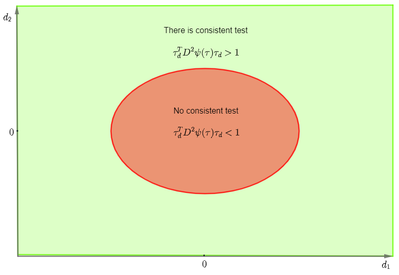
Theorem 2.2 says that, when $\bm{\tau}_{\bm{d}}^{T}D^{2}\psi(\bm{\tau})\bm{\tau}_{\bm{d}}<1$, any statistical test for (7) cannot achieve asymptotic power one. When $\bm{\tau}_{\bm{d}}^{T}D^{2}\psi(\bm{\tau})\bm{\tau}_{\bm{d}}>1$, the WSLMC test is consistent and hence optimal in this sense. The solution set $\{\bm{d}:\bm{\tau}_{\bm{d}}^{T}D^{2}\psi(\bm{\tau})\bm{\tau}_{\bm{d}}=1\}$ is an elliptic curve in $\bm{d}$, which is the sharp boundary for the existence of a consistent test. When $m=2$, these regions are demonstrated in Figure 1.

We point out the WSLMC test is not directly applicable in practice, since the vector $\bm{\tau}_{\bm{d}}$ and the function $\bm{T}(x)=(T_{1}(x),T_{2}(x),\dots,T_{m}(x))^{T}$ are unknown. Our results only provide some theoretical insights and serve as a benchmark for developing practical statistical tests. Motivated by $\mathcal{Z}_{n}$, more practical tests shall be proposed in Section 3.

Next, we illustrate our results by restricting $P,Q$ to the exponential distribution and the normal distribution.

Theorem 2.2 assumes the dimension $m$ of the exponential family to be finite. Actually, Theorem 2.2 holds even for infinite-dimensional exponential family defined in [15]:

where $\mathcal{F}$ is a subspace of a reproducing kernel Hilbert space $\mathcal{H}$, $q_{0}(x)$ is a reference density function and

The infinite-dimensional exponential family includes a very broad class of distributions (see [15, 28]).

Assume $P,Q\in\mathcal{P}$ are parametrized by $f_{1}$ and $f_{2}$ respectively. Let

where $g\in\mathcal{F}$ such that $f_{1},f_{2}\in\mathcal{F}$. Then the hypotheses (1) can be reformulated as follows:

where $\|g\|_{\mathcal{H}}$ represents the norm of $g$ in the Hilbert space $\mathcal{H}$. In this case, the WSLMC test has the following form:

where $\mathbb{E}_{f}$ represents expectation with respect to density $p_{f}(x)\in\mathcal{P}$.

To prove Theorem 2.3, one needs to replace the partial derivatives by Fr$\acute{e}$chet derivatives, and follows the line of proof of Theorem 2.2. In this sense, our result is pretty general.

Existing community detection algorithms and statistical tests for community structure are mainly developed for binary edges ([3, 4, 6, 8, 10, 11, 17, 19, 20, 23, 31, 39, 8]). When a network is weighted, a common way is to convert the weighted network to a binary one. It has been empirically verified that there is information loss in the dichotomizing process ([1, 2, 29]). However, it is unclear how much information is lost quantitatively. In this subsection, we provide the first formal quantification of information loss in the context of hypothesis testing via statistical limits.

Given a fixed real number $t_{0}$, the weights $A_{ij},i<j$ can be naturally dichotomized to binary ones $\tilde{A}_{ij}$ as follows

That is, all the weights smaller than $t_{0}$ are discarded and weights larger than $t_{0}$ are converted to ones ([1, 2, 29]). In this way, the weighted work $A$ is converted to an unweighted network $\tilde{A}$. The network $\tilde{A}$ inherits the community structure of $A$. Given $\bm{\sigma}$ and $\bm{\theta}(\sigma_{i},\sigma_{j})=\bm{\tau}-\frac{\bm{\tau}_{\bm{d}}}{\sqrt{n}}\sigma_{i}\sigma_{j}$, the probability of the presence of an edge in $\tilde{A}$ is

Hence, the hypotheses are still the same as (7). Under $H_{0}$, there is no community structure and the edge presence probability is

To get the sharp testing limit, we propose the signed-long-cycle (SLC) test statistic $\mathcal{R}_{n}$ as

The SLC test rejects $H_{0}$ if $|\mathcal{R}_{n}|>C$ for some constant $C$ dependent on the type I error.

For the dichotomized network, the sharp limit for existence of consistent test is given by the quantity $\frac{(\bm{a}(t_{0})^{T}\bm{\tau}_{\bm{d}})^{2}}{p_{0}(1-p_{0})}$. In general, $\frac{(\bm{a}(t_{0})^{T}\bm{\tau}_{\bm{d}})^{2}}{p_{0}(1-p_{0})}$ differs from $\bm{\tau}_{\bm{d}}^{T}D^{2}\psi(\bm{\tau})\bm{\tau}_{\bm{d}}$ in Theorem 2.2, since it depends on $t_{0}$. The difference between them can be considered as a measure of information loss incurred by dichotomizing a weighted network in the context of hypothesis testing. In this sense, our result provides the first theoretical characterization of loss of information.

In the general case, it is not immediately clearly what is the difference between $\frac{(\bm{a}(t_{0})^{T}\bm{\tau}_{\bm{d}})^{2}}{p_{0}(1-p_{0})}$ and $\bm{\tau}_{\bm{d}}^{T}D^{2}\psi(\bm{\tau})\bm{\tau}_{\bm{d}}$. For better illustration, we restrict $P,Q$ to be exponential distributions. In this case, $p_{0}=e^{-\tau t_{0}}$ , $a(t_{0})=t_{0}p_{0}$ and $\frac{(\bm{a}(t_{0})^{T}\bm{\tau}_{\bm{d}})^{2}}{p_{0}(1-p_{0})}=\frac{\tau^{2}t_{0}^{2}d^{2}}{e^{\tau t_{0}}-1}$. Then the following corollary follows.

For graphs with weights following the exponential distribution, the region without consistent test is $d^{2}<1$ by Example 1. For the dichotomized network, the region without consistent test is $d^{2}<\frac{e^{\tau t_{0}}-1}{\tau^{2}t_{0}^{2}}$ by Corollary 2.5. Note that $\min_{x>0}\frac{e^{x}-1}{x^{2}}=1.544$ as shown in Figure 2. Hence, $\frac{e^{\tau t_{0}}-1}{\tau^{2}t_{0}^{2}}\geq 1.544>1$ for any $\tau t_{0}>0$ and dichotomizing weighted exponential network to binary network always enlarges the region where no consistent test exists. This reflects the loss of information. For fixed $\tau$, $t_{0}=\frac{1.594}{\tau}$ leads to the least loss of information. This interesting finding theoretically confirms the intuition that the dichotomy threshold should not be too small or too large.

The result (I) in Theorem 2.2 only guarantees the inconsistency of any statistical test, without providing further description of their performances. This can actually be made stronger under an additional ODE condition. The following theorem says that, under such a condition, all tests perform not better than random guess.

The following example provides distributions that satisfy condition (8).

In this subsection, we illustrate the performance of the proposed tests and compare them with the spectral test ([30]) in various simulations. The nominal type I error is set to be 0.05. The empirical type I errors and powers are calculated based on 500 repetitions.

For each $l\in\{1,2,\dots,m\}$, the spectral test statistics are defined as

where

Note that $\Lambda_{n,1}$ is given in [30]. The rejection threshold is calculated based on the Tracy-Widom law with degree of freedom one.

We assess the performance of the cycle-based tests $\mathcal{T}_{n}$, $\mathcal{T}_{n,1}$, $\mathcal{T}_{n,2}$ and the spectral tests $\Lambda_{n,1},\Lambda_{n,2}$. The results for $\Lambda_{n}$ are not reported due to large type I errors. The random labels $\sigma_{i}$ $(1\leq i\leq n)$ are generated from Bernoulli distribution with success probability 0.5. Given $\bm{\sigma}=(\sigma_{1},\sigma_{2},\dots,\sigma_{n})$, let $\bm{\lambda}=(\lambda_{1},\lambda_{2})$ and $\bm{\epsilon}=(\epsilon_{1},\epsilon_{2})$, and

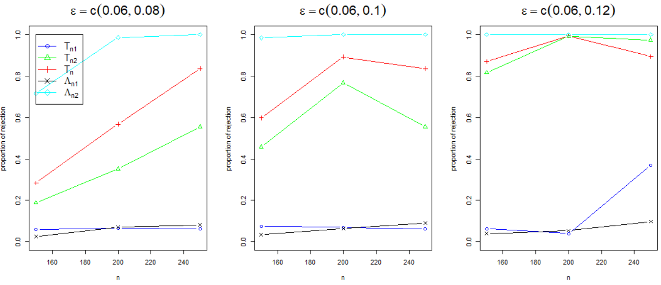
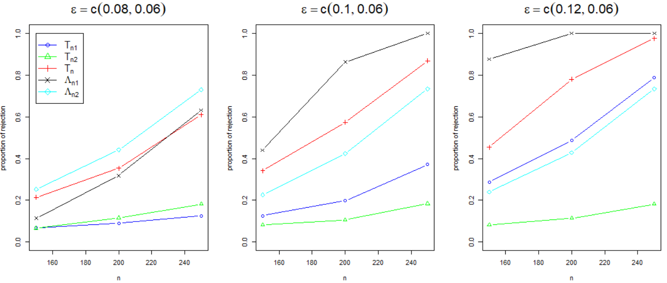
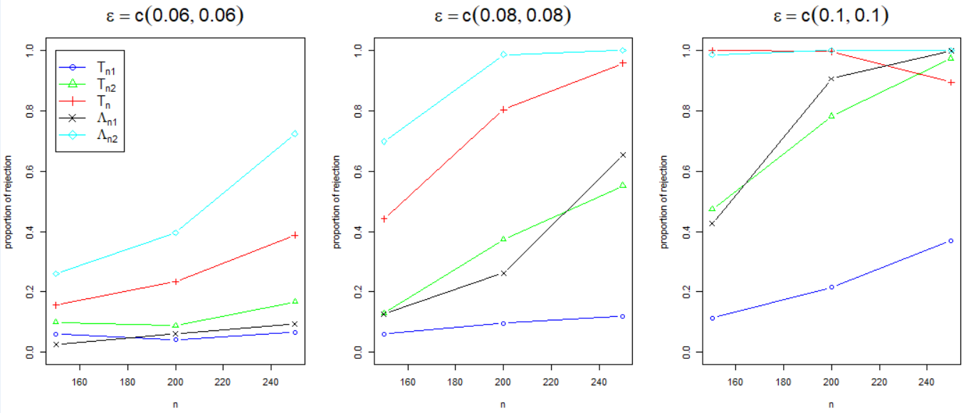
In the first simulation, we generate the weights from the normal distribution with mean $\mu_{1}$ and second moment $\mu_{2}$ defined in (10). Figure 3 summarizes the empirical type I errors and Figure 4 visualizes the powers.

In the second simulation, the weights are assumed to follow the Gamma distribution with mean and second moment given in (10). The density of Gamma distribution is given by

where $\lambda,\theta$ are functions of $\mu_{1},\mu_{2}$:

Figure 3 presents the empirical type I errors and Figure 5 plots the powers.

In the last simulation, we generate weights from the mixture of two exponential distributions with density given by

where

Note that this distribution does not belong to exponential family. The empirical type I errors are plotted in Figure 3 and Figure 6 visualizes the powers.

This simulation study has the following indications: $(I)$ The cycle-based tests with $k=3$ converge much faster than the spectral tests for non-Gaussian weights, since the cycle-based tests have empirical type I errors close to the nominal for smaller $n$. $(II)$ The empirical powers increase as the differences ($\epsilon_{1}$ or $\epsilon_{2}$) of parameters get larger. $(III)$ No single test can dominate the others in all cases. In summary, this simulation highlights the necessity to incorporate higher order moments of weights in test statistic and the proposed tests have significant advantage over spectral tests for smaller $n$.

In this subsection, we apply the proposed tests to an animal social network “aves-wildbird-network-5” publicly available at [26]. In this network, each bird is a node and edges are weighted by interaction between two birds. This network has 145 nodes and 2512 weighted edges. We apply test statistics $\mathcal{T}_{n}$, $\mathcal{T}_{n,1}$, $\mathcal{T}_{n,2}$ with $k=3$ to this network and the calculated test statistics are listed in Table 1. With type I error $0.05$, all these three tests reject the null hypothesis, which indicates the network contains community structure.

For the proof of part (I) of Theorem 2.2, we will use the second moment methods. Specifically, we show that the second moment of the likelihood ratio under $H_{0}$ is bounded if $2\sum_{|\alpha|=2}\frac{\partial^{\alpha}\psi}{\alpha!}(\bm{\tau})\left(\bm{\tau}_{\bm{d}}\right)^{\alpha}<1$. For the proof of part (II) of Theorem 2.2, we prove the WSLMC test has asymptotic power one if $2\sum_{|\alpha|=2}\frac{\partial^{\alpha}\psi}{\alpha!}(\bm{\tau})\left(\bm{\tau}_{\bm{d}}\right)^{\alpha}>1$. For convenience, we will let $m=2$. The proof for general $m$ is exactly the same as $m=2$.

References

• [1] Aicher, C. (2014). The Weighted Stochastic Block Model. Applied Mathematics Graduate Theses & Dissertations, 50.
• [2] Aicher, C., Jacob, A. and Clauset, A.(2015). Learning Latent Block Structure in Weighted Networks. Journal of Complex Networks, 3, 221-248.
• [3] Abbe, E. (2017). Community detection and stochastic block models: recent developments. Journal of Machine Learning Research, 18, 1-86.
• [4] Arias-Castro, E. and N. Verzelen. 2014. Community detection in dense random networks. Annals of Statistics, 42, 3: 940-969.
• [5] Ahn, K., Lee, K. and Suh, C.(2018). Hypergraph spectral clustering in the weighted stochastic block model. IEEE Journal of Selected Topics in Signal Processing. 12, 959-974.
• [6] Abbe, E. and Sandon, C. (2017). Proof of the achievability conjectures for the general stochastic block model. Communications on Pure and Applied Mathematics, 71(7), 1334-1406.
• [7] Abbe, E., Banderira, A. and Hall, G.(2016). Exact Recovery in the Stochastic Block Model. IEEE transactions on information theory, 62(1) 471-487.
• [8] Amini, A., Chen, A. and Bickel, P. (2013). Pseudo-likelihood methods for community detection in large sparse networks. Annals of Statistics, 41(4), 2097-2122.
• [9] Banerjee, D. (2018). Contiguity and non-reconstruction results for planted partition models: the dense case. Electronic Journal of Probability, 23, 1-28.
• [10] Banerjee, D. and Ma, Z. (2017). Optimal hypothesis testing for stochastic block models with growing degrees. https://arxiv.org/pdf/1705.05305.pdf.
• [11] Bickel, P. J. and Sarkar, P. (2016). Hypothesis testing for automated community detection in networks. Journal of Royal Statistical Society, Series B, 78, 253-273.
• [12] Bubeck,S., Ding, J., Eldan,R. and Rácz, M.(2016) Testing for high‐dimensional geometry in random graphs. Random Structures & Algorithms, 49(3),503-532.
• [13] Chen, J. and Yuan,B. (2006). Detecting functional modules in the yeast proteinprotein interaction network. Bioinformatics, 22(18), 2283-2290.
• [14] Colizza, V., Pastor-Satorras, R. and Vespignani, A.(2007). Reaction–diffusion processes and metapopulation models in heterogeneous networks. Nature Phys, 3, 276–282.
• [15] Canu, S. and Smola, A. J.(2005). Kernel methods and the exponential family. Neurocomputing, 69: 714–720.
• [16] Fortunato,S. (2010). Community detection in graphs. Physics Reports, 486 (3-5), 75-174.
• [17] Gao, C. and Lafferty, J. (2017a). Testing for global network structure using small subgraph statistics. https://arxiv.org/pdf/1710.00862.pdf
• [18] Jin,J., Ke, Z. and Luo S.(2018). Network global testing by counting graphlets. International conference on machine learning, 2333-2341.
• [19] Lei, J. (2016). A goodness-of-fit test for stochastic block models. Annals of Statistics, 44, 401-424.
• [20] Lei, J. and Rinaldo, A. (2015). Consistency of spectral clustering in stochastic block models. The Annals of Statistics, 43(1), 215-237.
• [21] Lu, Z., Wen, Y. and Cao, G.(2015). Community detection in weighted networks: algorithms and applications. IEEE Transactions on Parallel and Distributed Systems, 26(11): 2916-2926.
• [22] Mossel, E., Neeman, J. and Sly, A. (2015). Reconstruction and estimation in the planted partition model. Probability Theory and Related Fields, 162, 431-461.
• [23] Montanari, A. and Sen, S. (2016). Semidefinite programs on sparse random graphs and their application to community detection. STOC ’16 Proceedings of the forty-eighth annual ACM symposium on Theory of Computing, 814-827.
• [24] Newman, M. (2001). Scientific collaboration networks. I. Network construction and fundamental results. Physical Review E, 64, 016-131.
• [25] C. Nicolini, C. Bordier, and A. Bifone. Community detection in weighted brain connectivity networks beyond the resolution limit. Phys. Rev. E, 146:28–39, 2017.
• [26] R. Rossi and N. Ahmed. (2015).The Network Data Repository with Interactive Graph Analytics and Visualization, https://networkrepository.com.
• [27] M. Rubinov and O. Sporns. Complex network measures of brain connectivity: Uses and interpretations. NeuroImage, 52:1059–1069, 2010.
• [28] Sriperumbudur, B., Fukumizu, K., Gretton, A., Hyvarinen, A. adn Kumar,R.(2017). Density estimation in infinite dimensional exponential families,Journal of Machine Learning Research, 18,1-59.
• [29] Thomas, A. C. and Blitzstein, J. K. (2011). Valued ties tell fewer lies: Why not to dichotomize network edges with thresholds. arXiv:1101.0788
• [30] Tokuda, T. (2018). Statistical test for detecting community structure in real-valued edgeweighted graphs. PLoS ONE 13(3): e0194079.
• [31] Verzelen, N., and E. Arias-Castro. 2015. Community detection in sparse random networks. Ann. Appl. Probab. 25,6:3465–3510.
• [32] Xu,M., Jog, V. and Loh,P.(2020). Optimal rates for community estimation in the weighted stochastic block model. Annals of Statistics, 48(1):183-204.
• [33] Yuan, M., Feng,Y. and Shang, Z.(2022). A likelihood-ratio type test for stochastic block models with bounded degrees. Journal of Statistical Planning and Inference, 219:98-119.
• [34] Yuan, M., Yang, F. and Shang, Z. (2022). Hypothesis testing in sparse weighted stochastic block model. Statistical Papers, accepted.
• [35] Yuan, M., Liu, R., Feng, Y. and Shang, Z. (2022). Testing community structures for hypergraphs. Annals of Statistics, 50(1): 147-169.
• [36] Yuan, M. and Nan, Y. (2020). Test dense subgraphs in sparse uniform hypergraph. Communications in Statistics - Theory and Methods, to appear.
• [37] Yuan, M. and Shang, Z. (2021). Sharp Detection Boundaries on Testing Dense Subhypergraph.Bernoulli, to appear.
• [38] Zhao, Y., Levina, E. and Zhu., J.(2011). Community extraction for social networks. Proc. Natn. Acad. Sci. USA, 108, 7321-7326.
• [39] Zhao, Y., Levina, E. and Zhu, J. (2012). Consistency of community detection in networks under degree-corrected stochastic block models. Annals of Statistics, 40, 2266-2292.