Binary Multi Channel Morphological Neural Network

Let $\mathbb{N}^{*}$ be the set of non zero natural integers. Let $d\in\mathbb{N}^{*}$ the dimension of the image (usually $d=2$ or $d=3$). If $a\leq b\in\mathbb{Z}$, we denote the discrete interval as $[\![a,b]\!]=[a,b]\cap\mathbb{Z}$. Let $N_{I}\in\mathbb{N}^{*}$ and $\Omega_{I}=[\![-N_{I},N_{I}]\!]^{d}$ be the support of binary images $I\subset\Omega_{I}$. Let $\Omega_{S}=[\![-N_{S},N_{S}]\!]^{d}$ be the support of structuring elements (short: SE) $S\subset\Omega_{S}$. If $X\subset\mathbb{Z}^{d}$, we denote $\check{X}=\{-x\penalty\ |\penalty\ x\in X\}$ the symmetric of $X$ with respect to the origin. For a binary image $I\subset\Omega_{I}$, we define its complementation $I^{C}=\Omega_{I}\penalty\ \backslash\penalty\ I$. For a SE $S\subset\Omega_{S}$, if there is no ambiguity, we define its complementation as $S^{C}=\Omega_{S}\penalty\ \backslash\penalty\ S$. For a set $X\subset\mathbb{Z}^{d}$, we denote its indicator function $\mathbbm{1}_{X}:\mathbb{Z}^{d}\mapsto\mathbb{R}$ such that $\mathbbm{1}_{X}(x)=1$ if $x\in X$, else $\mathbbm{1}_{X}(x)=0$. If $\mathbbm{1}_{I}\in\mathbb{R}^{\Omega_{I}}$ and $\mathbbm{1}_{S}\in\mathbb{R}^{\Omega_{S}}$ we denote the convolutional product $\mathbbm{1}_{I}\circledast\mathbbm{1}_{S}:k\in\Omega_{I}\mapsto\sum_{i\in\Omega_{S}|k-i\in\Omega_{I}}(\mathbbm{1}_{I}(k-i)\mathbbm{1}_{S}(i)))$.

While not exhaustive, this list is representative of many useful morphological operators. These operators are obtained through composition and intersection or union of dilations, erosions, anti-dilations, and anti-erosions. Therefore, it is enough to learn these elementary operations, their SEs, and their aggregation.

First, we design a single neuron that replaces the convolution operation: it can learn the dilation, erosion, anti-dilation, anti-erosion, and their SEs.

One strength of ConvNets is their ability to learn multiple filters per layer, which we also want to ensure. In a convolutional layer, each final channel is a sum of one filter per input channel. In our case, the final result is either a union or an intersection of the elementary operators (dilation, erosion, anti-dilation, anti-erosion). Therefore, we want a layer that can learn the union or intersection of any combination of inputs. Let us consider $n$ binary images $x_{1},...,x_{n}\subset\Omega$. Let $\mathcal{C}\subset[\![1,n]\!]$. Then the intersection and union are given as:

As with the BiSE, we can use a single scalar to discriminate between the union or the intersection. To learn the set $\mathcal{C}$, we can use a parameter $\beta_{i}$ for each image. The following definition ensues:

A LUI layer can learn any intersection or union of any number of almost binary inputs. It is a particular case of BiSE layer. In this case, the SE support would be $\Omega_{lui}=\{0\}^{d}\times[\![1,n]\!]$. Learning the intersection is equivalent to learning an erosion, and learning the union is equivalent to learning a dilation. Then, we can deduce the following Theorem, by using the BiSE Theorem 2.1. We denote by $\mathcal{I}=\bigtimes_{k=1}^{n}{\mathcal{I}(u_{k},v_{k})}$ the set of images with $n$ almost binary channels.

As for the BiSE, if the LUI is activated, the set $\mathcal{C}$ can be found by thresholding the $(\beta_{k})_{k}$ for a specific value. If the LUI is not activated, it is still possible to binarize with the same method described for the BiSE in section 2.2.

We combine the BiSE neurons and the LUI in order to be able to learn the morphological operators and aggregate them as unions or intersections.

If the BiSEL is activated, given almost binary inputs, the outputs of the BiSEL are also almost binary.

The BiSEL follows the same logic as a convolutional layer. In ConvNets, at each layer, we have $k$ filters. Each filter applies one convolution to each channel, and then we apply a linear combination to all convoluted channels. In BiSEL, we have $K$ filters (the number of LUI). For each filter, we apply a morphological operation to a channel, and then we aggregate by taking the intersection or union of any channels. A schema of BiSEL can be found in figure 1.

Binarizing a BiSEL is equivalent to binarizing each of its element. If an element is activated, it is easy to binarize it. For those who are not, we must approximate them.

The parameters are the BiSE weights $\{W_{n,k}\}_{n,k}\subset\mathbb{R}^{\Omega_{S}}$, the BiSE biases $\{b_{n,k}\}_{n,k}\subset\mathbb{R}$, the LUI parameters $\{\beta_{n,k}\}_{n,k}\subset\mathbb{R}$ and the LUI biases $\{b^{l}_{k}\}_{k}\subset\mathbb{R}$. There are $N\cdot K(|\Omega_{S}|+2)+K$ parameters.

The BiSEL is akin to a complete convolution layer with multiple filters. We can simply stack multiple BiSELs to create a network similar to a convolutional neural network.

The BiMoNN can learn the composition of any intersection or union of dilation, erosion, anti-dilation, and anti-erosion. That includes but is not limited to opening, closing, black top-hat, and white top-hat.

There are two drawbacks to our current formulation. First, the input has the same dimension as the output. ConvNets can be combined in multi-scale architectures, which compresses the data. Currently, we cannot solve classification tasks with our method. Second, we can only learn predeternined composition of operators. However, some morphological operators like skeletonization or reconstruction need an undetermined number of iterations before convergence. Incorporating these features is left for further work.

We will be using the three datasets described in [2]: Diskorect, a set of custom-generated images composed of ellipses and rectangles that create as many different situations as possible; thresholded MNIST upsized to $50\times 50$, and its complementation that we call inverted MNIST. Examples are shown in figure 3.

Axial Spondyloarthritis (axSpA) is the most common auto-immune rheumatic disease. It is painful and debilitating if untreated or incorrectly diagnosed. The disease can be detected using MRIs: the inflammation is located on the sacroiliac joint. Given the sacrum and the iliac shapes, the task is to detect this joint region. We call this task axSpA.

The dataset is composed of around 1100 images with categorical images of size about $512\times 512$ with two values: one for the iliac and one for the sacrum. We transform them into binary images by separating each categorical value into one channel: final images have 2 channels. The target is defined as the joint region. Let $S_{a}=[\![-20,20]\!]\times\{0\}$. The target operation is $\gamma_{a}:X\in\{0,1\}^{512\times 512\times 2}=(X_{1}\oplus S_{a})\cap(X_{2}\oplus S_{a})$, with $X_{i}$ the $i-$channel. The resulting input-output couples are $\{(x_{i},\gamma_{a}(x_{i}))\penalty\ |\penalty\ x_{i}\in\text{axSpA dataset}\}$ (see figure 3(d)).

For dilation and erosion, the SEs are perfectly learned. The perfect DICE (=1) is reached in almost all cases. Even when the BiSEs are not activated, the approximate binarizations yield good results. Performance can decrease (see disk erosion on inverted MNIST), or increase (see disk erosion on MNIST).

On opening and closing, we reach perfect dice for most cases. All SEs can be seen on the code repository. We manage to recover the target SEs for most operations except on the opening on the inverted MNIST. We want to test the following hypothesis $\mathcal{H}$: dual operators learn similarly on dual datasets. On Diskorect, for any image $X$ in this dataset, then $X^{C}$ is also in it. Therefore $\mathcal{H}$ implies that opening and closing should have similar results. Already the hypothesis is rejected if we look at the stick opening vs. the stick closing: one succeeds and the other fails. On MNIST, $\mathcal{H}$ implies that the closing on MNIST should behave the same as the opening on inverted MNIST and vice versa. That is not observed and refutes further the hypothesis. Note that the model learns two anti-dilations for the closing, which is equivalent to learning dilation followed by erosion.

We compare our results to $\mathcal{L}Morph$ and $\mathcal{S}Morph$ [9]. They reach almost perfect DICE for erosion and dilation, but recovering the SEs from the learned weights is not straightforward. Moreover, on the opening and closing, the $\mathcal{L}Morph$ presents stability issues, and the $\mathcal{S}Morph$ fails to converge correctly to the proper operations. Those results are not surprising as these networks were designed for grey-scale morphology.

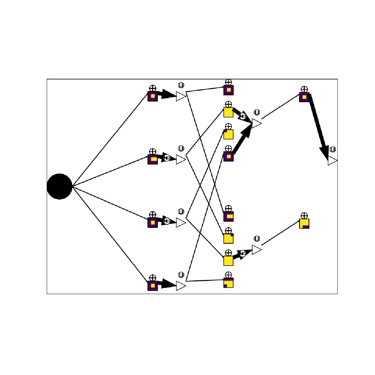
In this section, we study the model’s ability to learn the complementation and intersection with top-hat transform. We manage to learn the black top-hat for the Diskorect and inverted MNIST. For the cross, the binarization is perfect (see figure 4). The upper branch learns the complementation of the identity, and the bottom branch learns the closing with two sequential anti-dilations. The white top-hat only worked on Diskorect. The binarization decreases performance.

We attempt to learn the joint region. We want to learn the intersection of two dilations of size $41\times 41$. We try three different architectures that can theoretically learn this operation (see figure 5). They go from wide and shallow to deeper and narrower. Architectures 1 and 2 learn the operation well, reaching an excellent DICE ($1$ and $0.9$). Architecture 1’s weights are close to the target, and the binarization yields good results (DICE=$0.98$). On the other hand, architecture 2 learns wider dilations, and its binarization is quite bad (DICE=$0.7$). Note that there are multiple ways for this architecture to learn the target. Finally, the deeper network failed to learn anything. That may be due to the initialization: the output is constant and stuck in a zero-grad zone, which is a case of vanishing gradient. This application is hopeful in the study of axSpA. This model could be used with classical convolutional neural networks to improve MRI analysis by exploiting the ROI’s detection using segmentation results.

References

- [1] Angulo, J.: Some open questions on morphological operators and representations in the deep learning era. In: International Conference on Discrete Geometry and Mathematical Morphology. pp. 3–19. Springer (2021)
- [2] Aouad, T., Talbot, H.: Binary morphological neural network. arXiv preprint arXiv:2203.12337 (2022)
- [3] Dice, L.R.: Measures of the amount of ecologic association between species. Ecology 26(3), 297–302 (1945)
- [4] Franchi, G., Fehri, A., Yao, A.: Deep morphological networks. Pattern Recognition 102, 107246 (2020)
- [5] Glorot, X., Bengio, Y.: Understanding the difficulty of training deep feedforward neural networks. In: Proceedings of the thirteenth international conference on artificial intelligence and statistics. pp. 249–256. JMLR Workshop and Conference Proceedings (2010)
- [6] Hubara, I., Courbariaux, M., Soudry, D., El-Yaniv, R., Bengio, Y.: Binarized neural networks. Advances in neural information processing systems 29 (2016)
- [7] Kim, M., Smaragdis, P.: Bitwise neural networks. arXiv preprint arXiv:1601.06071 (2016)
- [8] Kingma, D.P., Ba, J.: Adam: A method for stochastic optimization (2017)
- [9] Kirszenberg, A., Tochon, G., Puybareau, É., Angulo, J.: Going beyond p-convolutions to learn grayscale morphological operators. In: International Conference on Discrete Geometry and Mathematical Morphology. pp. 470–482. Springer (2021)
- [10] Masci, J., Angulo, J., Schmidhuber, J.: A learning framework for morphological operators using counter–harmonic mean. In: International Symposium on Mathematical Morphology and Its Applications to Signal and Image Processing. pp. 329–340. Springer (2013)
- [11] Milletari, F., Navab, N., Ahmadi, S.A.: V-net: Fully convolutional neural networks for volumetric medical image segmentation (2016)
- [12] Mondal, R., Dey, M.S., Chanda, B.: Image restoration by learning morphological opening-closing network. Mathematical Morphology-Theory and Applications 4(1), 87–107 (2020)
- [13] Rumelhart, D.E., Hinton, G.E., Williams, R.J.: Learning Representations by Back-propagating Errors. Nature 323(6088), 533–536 (1986). https://doi.org/10.1038/323533a0, http://www.nature.com/articles/323533a0
- [14] Shen, Y., Zhong, X., Shih, F.Y.: Deep morphological neural networks. arXiv preprint arXiv:1909.01532 (2019)
- [15] Simons, T., Lee, D.J.: A review of binarized neural networks. Electronics 8(6), 661 (2019)