An Efficient Algorithm for the Proximity Connected Two Center Problem

The $k$-center problem in the plane is a fundamental facility-location problem in which we are given a set of $n$ demand points $P$ and we are going to find a set $S$ of $k$ center points such that $cost(S):=\max_{p\in P}\min_{s\in S}dist(p,s)$ is minimized ($dist(p,s)$ is the Euclidean distance between $p$ and $s$). The $k$-center problem is known to be NP-hard [3]. However, there is a simple greedy $2$-approximation algorithm for the problem which can not be improved unless $P=NP$ [3]. So, the studies on the problem went in the direction of obtaining polynomial-time algorithms where $k$ is not considered as a part of the problem input. As an example, in 2002, Agarwal and Procopiuc [1] gave a $n^{O(\sqrt{k})}$ time algorithm to solve the $k$-center problem. Solving the problem for specific values of $k$ like $k=1$ and $k=2$ received attention due to the geometric properties that can be applied to solve these problems efficiently. The $1$-center problem is indeed equivalent to the problem of covering $P$ with a disk with minimum area. This problem is also called the minimum enclosing disk (MED) problem. In 1983, Megiddo [24] used the prune and search technique to give an optimal linear time algorithm to solve the MED problem.

For $k=2$, Drenzer [10] gave the first nontrivial algorithm for the problem with $O(n^{3})$ time complexity. Later in 1994, Agarwal and Sharir [2] improved the time complexity for the problem to $O(n^{2}\log^{3}n)$. In 1996, Eppstein [11] gave a randomized algorithm for the problem with $O(n\log^{2}n)$ expected running time. In 1997, Katz and Sharir [20] proposed the novel expander-based parametric search technique and showed that applying it to the $2$-center problem using the $O(n^{2})$ time feasibility test of Hershberger [13], gives an $O(n^{2}\log^{3}n)$ time algorithm for the problem. Later in the year, Sharir [27] designed an $O(n\log^{3}n)$ time algorithm for the decision version of the $2$-center problem using the breakthrough observation of breaking the problem into three separate cases(far distant, distant and nearby cases). Next, he parallelized the decision algorithm and put it into the Megiddo’s parametric search schema [25] to obtain an $O(n\log^{9}n)$ time algorithm. Soon, it turned out that solving the problem in the nearby case is the bottleneck to reduce the time complexity. Later, Sharir’s running time was improved by Chan [5] and Wang [29] to $O(n\log^{2}n\log^{2}\log n)$ and $O(n\log^{2}n)$ respectively. Very recently, Choi and Ahn [8] (independently Cho and Oh [7]) obtained an $O(n\log n)$ time algorithm for the nearby case which led to an optimal $O(n\log n)$ time algorithm for the $2$-center problem.

We say that a set $S$ of $k$ center points in the plane satisfies the proximity connectedness condition (PCC) with respect to a parameter $\delta$ if the $\delta$-distance graph of $S$ (the graph with vertex set $S$ such that there is an edge between two vertices if and only if the distance between them is at most $\delta$) is connected. The proximity connected $k$-center problem is defined as a generalized version of the $k$-center problem for which, in addition to $P$, a parameter $\delta\geq 0$ is also given. The objective is to find $k$ center points $S$ such that $S$ satisfies the PCC and $cost(S)\leq cost(S^{\prime})$ for any $k$ center points $S^{\prime}$ that satisfies PCC ($cost(S)$ is the same cost as in the $k$-center problem). Note that when $\delta$ tends to zero (resp. infinity), the problem reduces to the $1$-center (resp. $k$-center) problem. Also, when $\delta$ tends to zero and $k$ tends to infinity the problem becomes the Euclidean Steiner tree problem (connecting the points of $P$ by lines of minimum total length in such a way that any two points can be connected by the lines). This is because in this configuration, the centers should be placed along the lines of the minimum Steiner tree in order to minimize the cost. The Euclidean Steiner tree problem is also NP-hard but it has a PTAS approximation algorithm [4].

In practice, the parameter $\delta$ usually specifies the range for which one center can communicate with other centers. So, when $S$ satisfies the PCC, any pair of centers can communicate with each other via the other centers. The proximity connected $2$-center (PCTC) problem first emerged in the works of Huang [16] in 1992 while he was studying packet radio networks. In the network terminology, the PCTC problem is the problem of locating two wireless devices as close as possible to the demand points $P$ such that they can send/receive messages between each other. He originally gave an $O(n^{5})$ time algorithm for the $2$-center problem having proximity constraints between their centers. Later in 2003, Huang et al. [18] studied a very close problem to the PCTC problem called $\alpha$-connected $2$-center problem. In this problem, instead of $\delta$, a parameter $0\leq\alpha\leq 1$ is given and the distance between the center of the disks should be at most $2(1-\alpha)r$ where $r$ is the radius of the disks. They gave an $O(n^{2}\log^{2}n)$ time algorithm for the decision version (given an $r$ whether it is possible to cover the points with two disks of radius $r$ satisfying the desired conditions) of the problem. Note that this problem is a special case of the PCTC decision problem where $\delta=2(1-\alpha)r$. Later in 2006, they gave a randomized algorithm with the same $O(n^{2}\log^{2}n)$ expected running time to solve the $\alpha$-connected $2$-center problem [17]. In this paper, we consider the PCTC problem and propose a deterministic $O(n^{2}\log n)$ time algorithm for it.

Here, we need to mention that although we use Sharir’s observation [27] of breaking the problem into three different cases(far distant, distant and nearby), the reason we can’t get a sub-quadratic algorithm like [27, 5, 29, 8] is that the PCTC problem is structurally different from the $2$-center problem. In the $2$-center problem, the optimal cost is determined by at most three points of $P$ [27] while in the PCTC problem the cost may be determined by more than three points because of the PCC. This means that our search space has a higher dimension than the search space of the $2$-center problem. Also, all the sub-quadratic algorithms for the $2$-center problem use Megiddo’s [25] or Cole’s [9] parametric search schema to reduce the time complexity which makes the resulting algorithm impractical [2] while our algorithm exploits the geometric properties of the problem which make it straightforward to be implemented using standard data structures in computational geometry.

A solution for a given PCTC problem instance is defined as a pair of disks whose centers satisfy the PCC and their union covers $P$. We call a disk with the larger (or equal) radius the determining disk of the solution and its radius the cost of the solution. An optimal solution is a solution with minimum cost among the set of all solutions for the problem. Note that there might be an infinite number of optimal solutions with different pairs of radii because we have freedom on the smaller disk. So, we try to find an optimal solution such that the radius of its smaller disk is minimum among all optimal solutions. We call such a solution a best optimal solution (BOS) for the problem. Therefore, if the problem has more than one BOS, they would have the same pair of radii. We can also compare two solutions $S_{1}$ and $S_{2}$ as follows: we say that $S_{1}$ is a better solution than $S_{2}$ if $cost(S_{1})<cost(S_{2})$ and if $cost(S_{1})=cost(S_{2})$, the radius of the non-determining disk of $S_{1}$ is smaller than the radius of the non-determining disk of $S_{2}$. In this paper, our algorithm not only gives us an optimal solution but it computes a BOS for the problem.

Let $(P,\delta)$ be the given PCTC problem instance where $P$ is a set of $n$ demand points in the plane and $\delta$ is a given non-negative number. We assume that the points are in general position, by which we mean no four points of $P$ lie on a circle. Let $(P_{1},P_{2})$ be a partition of $P$ obtained by dividing the plane by a line or two half-lines from a point (henceforth, when we use the term partition of the plane, we mean a partition that satisfies this condition). We say that a pair of disks $(D_{1},D_{2})$ with centers $(c_{1},c_{2})$ respectively is a solution for the partition if $D_{1}$ covers $P_{1}$, $D_{2}$ covers $P_{2}$ and $dist(c_{1},c_{2})\leq\delta$. Optimal and best optimal solutions (BOSs) for the partition are defined similarly. Let $(D^{*}_{1},D^{*}_{2})$ be a BOS for the partition with centers $(c^{*}_{1},c^{*}_{2})$ respectively. We say that a point $p\in P_{1}$ is a dominating point of $D^{*}_{1}$ if $(D^{*}_{1},D^{*}_{2})$ is not a BOS for the partition $(P_{1}\setminus p,P_{2})$. The dominating points of $D^{*}_{2}$ are defined similarly. Note that the dominating points of $D^{*}_{1}$ and $D^{*}_{2}$ are on their boundaries. By assuming that the points are in general position, if $D^{*}_{1}$(resp. $D^{*}_{2}$) is the MED of $P_{1}$(resp. $P_{2}$), its dominating points are either three points on the boundary such that their induced triangle contains $c^{*}_{1}$(resp. $c^{*}_{2}$) or two points on the boundary such that their connecting segment passes through $c^{*}_{1}$(resp. $c^{*}_{2}$). In order to simplify the presentation of our algorithm, in the latter case, we consider one of the dominating points as two infinitely close points and so, if $D^{*}_{1}$ or $D^{*}_{2}$ is the MED of their corresponding points, we assume that it has exactly three dominating points. Similarly, if $D^{*}_{1}$(resp. $D^{*}_{2}$) is not the MED of $P_{1}$(resp. $P_{2}$), in the case that it only has one dominating point, we can consider it as two infinitely close points. But, if it has three points on its boundary such that their induced triangle does not contain $c^{*}_{1}$, we might have no dominating point for $D^{*}_{1}$. We can assume that such a situation never happens by slightly perturbing the points. So, henceforth, if $D^{*}_{1}$(resp. $D^{*}_{2}$) is not a MED, we assume that it has exactly two dominating points.

We call the problem of computing a BOS for a given partition $(P_{1},P_{2})$ the restricted PCTC problem. In the next section, we show that how we can solve the restricted PCTC using the intersection hulls and the farthest-point Voronoi diagrams of $P_{1}$ and $P_{2}$ (the intersection hull of a set of points with respect to some radius $r$ is defined as the intersection of all disks of radius $r$ around the points of the set). See Appendix A for a review on farthest-point Voronoi diagrams and intersection hulls and their properties.

Let $(P_{1},P_{2})$ be a given partition. First, we compute the minimum enclosing disks $D_{1}^{**}$ and $D_{2}^{**}$ for $P_{1}$ and $P_{2}$ respectively. This can be done in linear time due to Megiddo’s algorithm [24]. Also let $c_{1}^{**}$ and $c_{2}^{**}$ be the centers of $D_{1}^{**}$ and $D_{2}^{**}$ respectively. Now, if $dist(c_{1}^{**},c_{2}^{**})$(the distance between $c_{1}^{**}$ and $c_{2}^{**}$) is at most $D$, then we are done and $(D_{1}^{**},D_{2}^{**})$ is a BOS for the partition. Otherwise, we have the following proposition:

Proof. We proceed by contradiction. Suppose that for an optimal solution $(D^{*}_{1},D^{*}_{2})$, $dist(c_{1}^{*},c_{2}^{*})<\delta$. So, at least one of the centers for example $c^{*}_{1}$ should be different from $c^{**}_{1}$ and lies inside the region between the two perpendicular lines from $c_{1}^{**}$ and $c_{2}^{**}$ on $line(c^{**}_{1},c^{**}_{2})$ (the line passing $c_{1}^{**}$ and $c_{2}^{**}$). This is because if both $c_{1}^{*}$ and $c_{2}^{*}$ are outside this region, the distance between them can’t be less than $\delta$. If $c^{*}_{1}$ is not on $\partial\mathcal{F}(P_{1})$, then we can slightly move $c^{*}_{1}$ toward its farthest point, reducing the radius of $D^{*}_{1}$ while not violating the PCC which contradicts best optimality. If $c_{1}^{*}$ is on $\partial\mathcal{F}(P_{1})$, by Proposition 7, any point on the interior of the path from $c_{1}^{**}$ to $c_{1}^{*}$ on $\partial\mathcal{F}(P_{1})$, covers $P_{1}$ with radius smaller than $r(D^{*}_{1})$. Since $dist(c^{*}_{1},c^{*}_{2})<\delta$, any point on this path sufficiently close to $c_{1}^{*}$ will not violate the PCC. This contradicts the fact that $(D^{*}_{1},D^{*}_{2})$ is a BOS.$\hfill\square$

Let $H_{1}(r)$ and $H_{2}(r)$ be the intersection hulls of $P_{1}$ and $P_{2}$ with radius $r$. Note that the smallest radii for which the intersection hulls of $P_{1}$ and $P_{2}$ are nonempty are $r(D_{1}^{**})$ and $r(D_{2}^{**})$ respectively. Let’s denote them by $r_{1}^{0}$ and $r_{2}^{0}$ (in fact $H_{1}(r_{1}^{0})=c_{1}^{**}$ and $H_{2}(r_{2}^{0})=c_{2}^{**}$). If $r\geq r_{1}^{0}$, for any point $q\in H_{1}(r)$, $disk(q,r)$(the disk with center $q$ and radius $r$) covers $P_{1}$ (we have a similar statement for $P_{2}$ and $r_{2}^{0}$). Based on this property, the problem turns to find a best optimal pair of radii $(r^{*}_{1},r^{*}_{2})$ (the bigger radius is minimum and the smaller radius is minimum among all such pairs) such that the distance between $H_{1}(r^{*}_{1})$ and $H_{2}(r^{*}_{2})$ is exactly $\delta$. Also, we call the maximum radius of optimal pair(s) the optimal cost and denote it by $r^{*}$. The idea to find a best optimal pair is first try to find the optimal cost $r^{*}$ and then, fix one of the intersection hulls at radius $r^{*}$ and find minimum possible radius for the other hull. So here, we focus on finding the optimal cost.

In order to find the optimal cost, we impose the constraint that the disks are congruent (radii of both hulls should be equal). Imposing this constraint makes the problem easier while it does not change the optimal cost. In order to solve the problem for congruent disks, we can grow the intersection hulls of the points at each part of the partition to see when the distance between them becomes $\delta$. We first build $\mathcal{F}(P_{1})$ and $\mathcal{F}(P_{2})$ which can be done in $O(n\log n)$ time. In order to prevent structural changes when we grow the intersection hulls, we apply a binary search (repeatedly find the median and discard half of the values) on the set of weights of the farthest-point Voronoi diagrams of both sides to obtain an interval $I^{*}=(i_{0},i_{1})$ such that $r^{*}\in I^{*}$ and for each vertex $v$ of the diagrams, $w(v)\notin I^{*}$ (the weight of a point $x$ in a cell of farthest-point Voronoi diagram denoted by $w(x)$ is the distance between $x$ and the site of the cell containing it. See Appendix A for details). At each step of the binary search, when we test a weight $w$, we use the algorithm of [6] to compute the distance between the two intersection hulls at radius $w$ to see whether their distance is smaller, equal or greater than $\delta$. Note that because the intersection hulls are convex, this step can be done in $O(\log n)$ time according to [6] (we don’t need to explicitely build the intersection hulls because their vertices are along the edges of the farthest-point Voronoi diagrams).

In other words, when $r$ varies from $i_{0}$ to $i_{1}$, no arc in intersection hulls will be emerged or vanished. Let’s denote the arms of $H_{1}(i_{0})$ by $A_{1}$ and call the partition induced by $H_{1}(i_{0})\cup A_{1}$ the $A_{1}$-partition of the plane. Now, we discuss how to find the optimal cost for the partition. Suppose that we have not found $r^{*}$ during the binary search (otherwise we are done). So, $dist(H_{1}(i_{0}),H_{2}(i_{0}))>\delta$ and $dist(H_{1}(i_{1}),H_{2}(i_{1}))<\delta$. Let $Seq(H_{1}(i_{0}))=(X_{1},\dots,X_{u})$ and $Seq(H_{2}(i_{0}))=(Y_{1},\dots,Y_{u^{\prime}})$. We also label each region of the $A_{1}$-partition bounded by two neighbour arms by the name of the arc it contains. Each arm in $A_{1}$ can intersect $\partial H_{2}(i_{0})$ in at most two points. Consider an arm in $A_{1}$ with endpoint $a$ and an intersection point $x$ with $\partial H_{2}(i_{0})$. We call this intersection point a first intersection point if $ax$ does not intersect the interior of $H_{2}(i_{0})$.

Let $B$ be the set of all first intersection points of the arms in $A_{1}$ and $\partial H_{2}(i_{0})$. Note that $H_{2}(i_{0})$ is convex and the arms around $H_{1}(i_{0})$ diverges from each other. Also, we already have the order of the arms around $H_{1}(i_{0})$ induced by $\mathcal{F}(P_{1})$. In order to compute $B$, consider the counter-clockwise order on the arms of $A_{1}$ starting from the arm with the lowest slope (can be negative) and compute their first intersection points with $H_{2}(i_{0})$ in order. An important point here is that if a vertex of $H_{2}(i_{0})$ lies on the right side of an arm $\vec{a}$ (the direction is from its endpoint), it will be on the right side of any arm after $\vec{a}$. This proprty implies that the cost of computing $B$ is linear (see Figure 1).

Now, consider the partition induced by $B$ and the vertices of $\partial H_{2}(i_{0})$ on $\partial H_{2}(i_{0})$. We call each region of this partition a mini-arc on $\partial H_{2}(i_{0})$ (see Figure 1).

We assign a label $(X_{i},Y_{j})$ to each mini-arc of $\partial H_{2}(i_{0})$ where $X_{i}$ is the label of the mini-arc in the $A_{1}$-partition and $Y_{j}$ is the label the arc of $H_{2}(i_{0})$ containing the mini-arc. Note that the number of such $(X_{i},Y_{j})$ labels are linear (because we have a linear number of mini-arcs).

Proof. Let $p_{1}$ and $p_{2}$ be two points on $H_{1}(r^{*})$ and $H_{2}(r^{*})$ respectively with distance $\delta$. First, we observe that the perpendicular lines on $line(p_{1},p_{2})$ from $p_{1}$ and $p_{2}$ should not intersect the interior of $H_{1}(r^{*})$ and $H_{2}(r^{*})$ (otherwise it contradicts the optimallity of $r^{*}$). Suppose that $p_{1}$ and $p_{2}$ are lie on two arcs $X_{i}$ and $Y_{j}$ respectively (we consider the names of the arcs in $H_{1}(r^{*})$ and $H_{2}(r^{*})$ the same as the label of their corresponding regions in $H_{1}(i_{0})$ and $H_{2}(i_{0})$ respectively). If $(X_{i},Y_{j})$ is not a label of a mini-arc, $p_{1}p_{2}$ should intersect an arm of $X_{i}$. But in this situation, the perpendicular line on $line(p_{1},p_{2})$ from $p_{1}$ should intersect the interior of $H_{1}(r^{*})$ (because of convexity of $H_{1}(r^{*})$) which is contradiction. See Figure 2. $\hfill\square$

According to Proposition 2, we can compute $r^{*}$ as follows: we consider each label $(X_{i},Y_{j})$ of the mini-arcs and compute the value $r_{i,j}$ for which the distance between the two arcs $X_{i}$ and $Y_{j}$ becomes $\delta$ as they propagate between their bounding arms. Note that computing each $r_{i,j}$ can be done in a constant time. Now, $r^{*}$ is the minimum value among all $r_{i,j}s$.

The next step is obtaining a BOS for the partition after computing $r^{*}$. As we said earlier, in order to do this, we first assume that the determining disk covers $P_{1}$ and obtain the minimum possible radius $r_{1}^{\prime}$ for $H_{2}$ which makes the distance between $H_{1}(r^{*})$ and $H_{2}(r^{\prime}_{1})$ exactly $\delta$. This can be done in a similar way to how we obtained $r^{*}$. Then we obtain $r_{2}^{\prime}$ similarly by assuming that the determining disk covers $P_{2}$. By comparing the results, we pick the one with smaller non-determining disk which is in fact a BOS for the partition. So, the total time we need to compute a BOS is $O(n\log n)$.

We denote the optimal cost for the PCTC problem by $r^{*}$ and a BOS for the problem by $(D^{*}_{1},D^{*}_{2})$ with centers $(c^{*}_{1},c^{*}_{2})$ respectively. We can assume that $c^{*}_{1}$ and $c^{*}_{2}$ lie on the $x$-axis and $c^{*}_{1}$ is on the left side of $c^{*}_{2}$. In [27], Sharir broke the $2$-center decision problem (given a parameter $r$ determine whether it is possible to cover the points with two disks of radius $r$) into three cases -far distant, distant and nearby- with respect to the given parameter $r$. He showed that providing separate algorithms for these cases will reduce the overall time complexity to solve the decision problem. Although our problem is an optimization problem and the parameter $r^{*}$ is unknown, we will show that breaking the PCTC problem into the same cases will simplify our algorithm and reduce the overall time complexity. So, our algorithm separately considers each of the following three assumptions about $(D^{*}_{1},D^{*}_{2})$.

1. 1.

   Nearby: $dist(c^{*}_{1},c^{*}_{2})\leq r^{*}$.

2. 2.

   Distant: $r^{*}<dist(c^{*}_{1},c^{*}_{2})\leq 3r^{*}$.

3. 3.

   Far distant: $dist(c^{*}_{1},c^{*}_{2})>3r^{*}$.

Denote the smallest cost we can get having the nearby, distant and far distant assumptions by $r^{NA}$, $r^{DA}$ and $r^{FA}$ respectively. We also use the same notation for a BOS and their corresponding centers having each assumption. So, we can obtain $(D^{*}_{1},D^{*}_{2})$ by comparing $(D^{NA}_{1},D^{NA}_{2})$, $(D^{DA}_{1},D^{DA}_{2})$ and $(D^{FA}_{1},D^{FA}_{2})$ (note that these solutions may not exist or satisfy their corresponding case conditions. For example, $dist(c^{NA}_{1},c^{NA}_{2})$ might be greater than $r^{NA}$ but if $(D^{*}_{1},D^{*}_{2})$ satisfies the nearby case, then $r^{NA}=r^{*}$ and $(D^{NA}_{1},D^{NA}_{2})$ would be a BOS for the problem and we have $dist(c^{NA}_{1},c^{NA}_{2})\leq r^{NA}=r^{*}$). Henceforth, while studing each of the cases, when we say BOS, we mean a best solution we can get having the corresponding case assumption. Given two points $x$ and $y$ in the plane, we denote the line passing from $x$ and $y$ by $line(x,y)$. The direction of this line is considered from $x$ to $y$. Also, we denote the half-line from $x$ passing $y$ by $half\text{-}line(x,y)$ and the line segment with end points $x$ and $y$ by $seg(x,y)$.

First, we can see that if $(D^{*}_{1},D^{*}_{2})\leq r^{*}$, then there is an optimal partition $R^{*}$ (may not be unique) such that $(D^{*}_{1},D^{*}_{2})$ is a BOS of $R^{*}$. In fact, such a partition can be obtained by considering a point in $D^{*}_{1}\cap D^{*}_{2}$ and two half-lines from it passing the intersection points of $\partial D^{*}_{1}$ (boundary of $D^{*}_{1}$) and $\partial D^{*}_{2}$. In this section, when we say the dominating points of $(D^{*}_{1},D^{*}_{2})$, we mean its dominating points with respect to $R^{*}$. Without loss of generality, we can assume that $D^{*}_{2}$ is the determining disk. We first compute the $convex\text{-}hull(P)$ and scale the problem such that it fits in a unit square (multiple both $x$ and $y$ coordinates of the points by the greatest constant such that the convex hull remains inside the square). This step can be done in $O(n\log n)$ time. Note that the scaling will not change the solutions.

Proof. We proceed by contradiction. Suppose that such a factor does not exist. This means that we can build a problem instance such that it has a BOS $(D^{*}_{1},D^{*}_{2})$ in which the radius of the non-determinig disk ($D^{*}_{1}$) becomes infinitely small (because of the nearby assumption and scaling). So, $D^{*}_{1}$ should have at least one dominating point that is not covered by $D^{*}_{2}$. Because the radius of $D^{*}_{1}$ is infinitely small, $\delta$ should tend to $radius(D^{*}_{2})$ (which tends to the radius of the MED of $P$). Now, $D^{*}_{2}$ should have at least one dominating point (point $c$ in Figure 3) with the $x$-coordinate less than or equal to $c^{*}_{2}$ (otherwise, we can move both $c^{*}_{1}$ and $c^{*}_{2}$ to the right and reduce the radius of $D^{*}_{2}$ which determines the cost). In this configuration, we can enlarge $D^{*}_{1}$ by moving $c^{*}_{1}$ toward this dominating point of $D^{*}_{2}$ while satisfying the PCC in order to cover it and release it from $D^{*}_{2}$ ($D^{*}_{1}$ does not lose any of its own points and its radius still remains less than the radius of $D^{*}_{2}$). Now, we can reduce the radius of $D^{*}_{2}$ which contradicts the optimallity of $(D^{*}_{1},D^{*}_{2})$ (see Figure 3).$\hfill\square$

See Appendix B for the proof. Considering the four dominating points in the above proposition, we can say that $D^{*}_{1}\cap D^{*}_{2}$ should cover at least a constant factor of the area of $convex\text{-}hull(P)$. Furthermore, $D^{*}_{1}\cap D^{*}_{2}\cap convex\text{-}hull(P)$ is convex because it is the intersection of convex objects. So, we can build a constant size set of points $\mathcal{M}$ uniformly distributed on $convex\text{-}hull(P)$ such that (assuming $dist(c^{*}_{1},c^{*}_{2})\leq r^{*}$) for at least one point $\hat{m}\in\mathcal{M}$, $\hat{m}\in D^{*}_{1}\cap D^{*}_{2}\cap convex\text{-}hull(P)$. Because $\hat{m}$ is unknown, for each $m\in\mathcal{M}$, we build a BOS $(D_{1}^{m},D_{2}^{m})$ assuming $m\in D_{1}^{*}\cap D_{2}^{*}$ and finally pick a best solution in $\{(D_{1}^{m},D_{2}^{m})\;:\;m\in\mathcal{M}\}$ and set it as $(D^{NA}_{1},D^{NA}_{2})$. Based on this idea, we present our algorithm to find $(D^{m}_{1},D^{m}_{2})$ for a given point $m\in convex\text{-}hull(P)$.

Let $\mathcal{X}$ be a set of $360$ directed lines (each line has a positive direction) passing through $m$ such that the angle between each directed line and its neighbour lines is $1^{\circ}$. Now, there should be a directed line in $\mathcal{X}$ such that its angel with $line(c^{*}_{1},c^{*}_{2})$ is at most $1^{\circ}$ and $c^{*}_{1}$ lies on the negative side of $c^{*}_{2}$ on the line (note that $D^{*}_{2}$ is the determining disk according to our assumption). We call this directed line the correct directed line which is unknown. So, we assume each line $l\in\mathcal{X}$ as the correct directed line and compute a BOS $(D^{m,l}_{1},D^{m,l}_{2})$ having this assumption and finally pick the best one as $(D^{m}_{1},D^{m}_{2})$.

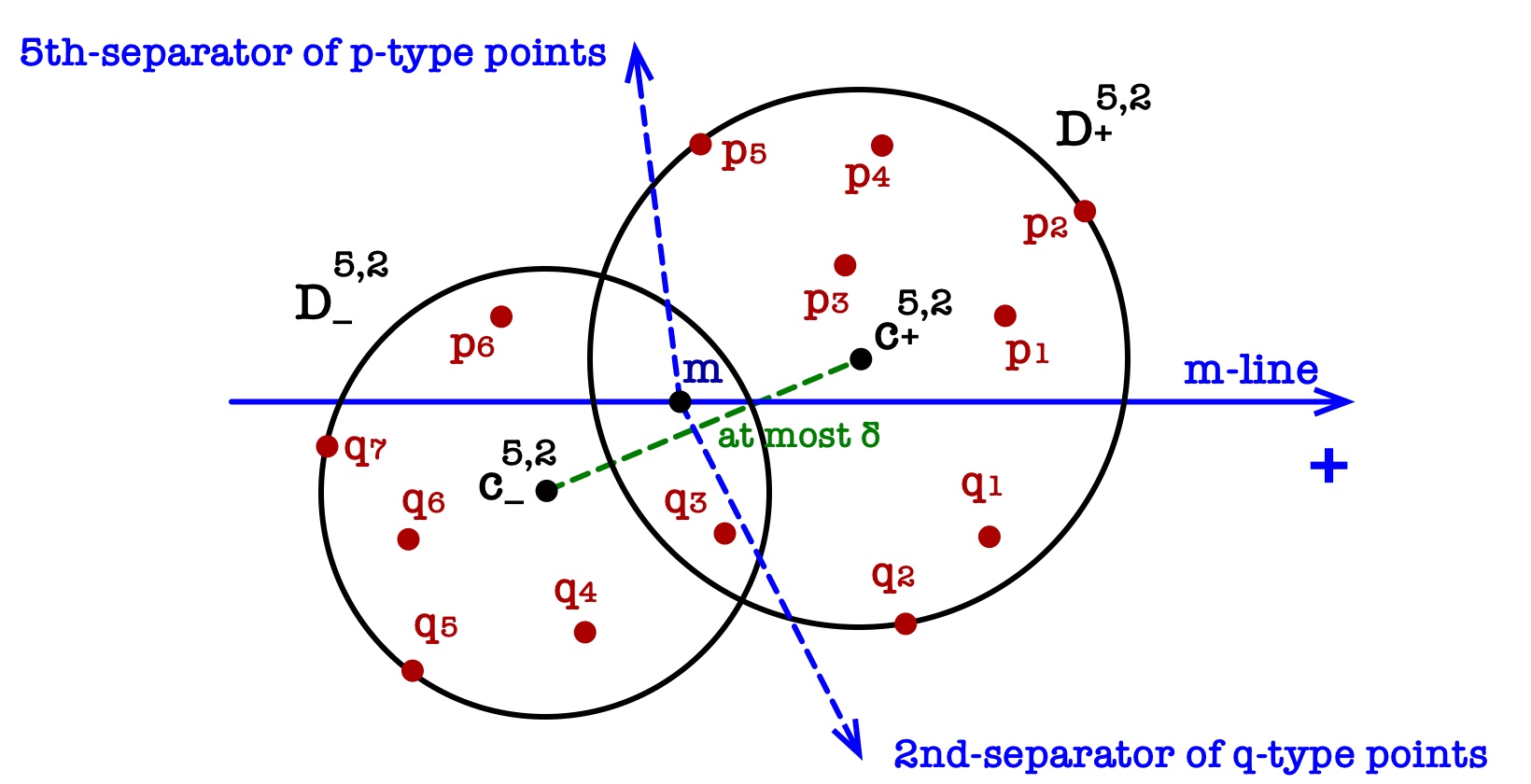
So, assume that a directed line $l\in\mathcal{X}$ called the $m$-line is given. Here we explain how to compute $(D^{m,l}_{1},D^{m,l}_{2})$. The $m$-line divides the points of $P$ into two disjoint sets one on the right side and the other on the left side of the $m$-line. We sort these sets according to the polar angles of their points (from $m$) with respect to the positive direction of the $m$-line. These angles should lie between $-180^{\circ}$ and $180^{\circ}$ and we sort them by increasing magnitude (see Figure 4 for an illustration). Based on these orders, we denote the two sequences of points on the left and right side of the $m$-line by $(p_{1},\dots,p_{n^{\prime}})$ and $(q_{1},\dots,q_{n^{\prime\prime}})$ respectively. We call a point $p\text{-}type$ (resp. $q\text{-}type$) if it is in the first(resp. second) sequence. We also call a half-line from $m$ that separates $\{p_{1},\dots,p_{i}\}$ from $\{p_{i+1},\dots,p_{n^{\prime}}\}$ an $i^{th}$-separator of the $p$-type points. A $j^{th}$-separator of $q$-type points is defined similarly (we assume that the $0^{th}$ and $n^{\prime th}$(resp. $n^{\prime\prime th}$) separators have the entire $p$-type(resp. $q$-type) points in one side). The $i^{th}$ and $j^{th}$ separators of the $p$-type and $q$-type points partition the plane into two parts. We call this partition the $(i,j)$-partition of the plane. One part of this partition contains the positive direction of the $m$-line which we call it the positive side of the partition and we call the other part the negative side of the partition.

Note that in the above observation, the two separators from $m$ passing the intersection points of $D^{*}_{1}$ and $D^{*}_{2}$ give us the desired $(i,j)$-partition. We denote the set of points in the positive and negative sides of the partition by $P^{i,j}_{+}$ and $P^{i,j}_{-}$ respectively. Based on our algorithm for restricted PCTC problem, a BOS for an $(i,j)$-partition can be computed in $O(n\log n)$ time. Let $(D^{i,j}_{-},D^{i,j}_{+})$ (with centers $(c^{i,j}_{-},c^{i,j}_{+})$ respectively) be the output of this algorithm for the $(i,j)$-partition (see Figure 4 for an example). We refer to the first(resp. second) disk the negative disk(resp. positive disk) of the partition. A naive approach to obtain $(D^{*}_{1},D^{*}_{2})$ is to apply our restricted PCTC problem algorithm to each of the $(i,j)$-partitions and pick the best one. This will give us an $O(n^{3}\log n)$ time complexity as there are quadratic partitions. In the following we show how we can get $(D^{m,l}_{1},D^{m,l}_{2})$ by evaluating a sub-quadratic number of partitions. The idea is first computing $r^{m,l}$ which is the best cost we can get assuming $m$ and $l$ are correct. Then, we use it to compute $(D^{m,l}_{1},D^{m,l}_{2})$.

References

- [1] Agarwal PK, Procopiuc CM. Exact and approximation algorithms for clustering. Algorithmica. 2002 Jun 1;33(2):201-26
- [2] Agarwal PK, Sharir M. Planar geometric location problems. Algorithmica. 1994 Feb;11(2):185-95.
- [3] Agarwal PK, Sharir M. Efficient algorithms for geometric optimization. ACM Computing Surveys (CSUR). 1998 Dec 1;30(4):412-58.
- [4] Arora S. Nearly linear time approximation schemes for Euclidean TSP and other geometric problems. In Proceedings 38th Annual Symposium on Foundations of Computer Science 1997 Oct 20 (pp. 554-563). IEEE.
- [5] Chan TM. More planar two-center algorithms. Computational Geometry. 1999 Sep 1;13(3):189-98.
- [6] Chin F. Optimal algorithms for the intersection and the minimum distance problems between planar polygons. IEEE Transactions on Computers. 1983 Dec 1(12):1203-7.
- [7] Cho K, Oh E. Optimal algorithm for the planar two-center problem. arXiv preprint arXiv:2007.08784. 2020 Jul 17
- [8] Choi J, Ahn HK. Efficient planar two-center algorithms. Computational Geometry. 2021 Apr 2:101768.
- [9] Cole R. Slowing down sorting networks to obtain faster sorting algorithms. Journal of the ACM (JACM). 1987 Jan 1;34(1):200-8.
- [10] Drezner Z. The planar two-center and two-median problems. Transportation Science. 1984 Nov;18(4):351-61.
- [11] Eppstein D. Faster construction of planar two-centers. In Proc. of the 8th Annual ACM-SIAM Symposium on Discrete Algorithms (SODA), pages 131–138, 1997.
- [12] Gudmundsson J, Haverkort H, Park SM, Shin CS, Wolff A. Facility location and the geometric minimum-diameter spanning tree. Computational Geometry. 2004 Jan 1;27(1):87-106.
- [13] Hershberger J. A faster algorithm for the two-center decision problem. Information processing letters. 1993 Aug 9;47(1):23-9.
- [14] Hershberger J, Suri S. Efficient computation of Euclidean shortest paths in the plane. In Proceedings of 1993 IEEE 34th Annual Foundations of Computer Science 1993 Nov 3 (pp. 508-517). IEEE.
- [15] Hershberger J, Suri S. Off-line maintenance of planar configurations. Journal of algorithms. 1996 Nov 1;21(3):453-75.
- [16] Huang CH. Some problems on radius-weighted model of packet radio network (Doctoral dissertation, Ph. D. Dissertation, Dept. of Comput. Sci., Tsing Hua Univ., Hsinchu, Taiwan).
- [17] Huang PH, Tsai YT, Tang CY. A near-quadratic algorithm for the alpha-connected two-center problem. Journal of information science and engineering. 2006 Nov 1;22(6):1317.
- [18] Huang PH, Te Tsai Y, Tang CY. A fast algorithm for the alpha-connected two-center decision problem. Information Processing Letters. 2003 Feb 28;85(4):205-10.
- [19] Hwang RZ, Lee RC, Chang RC. The slab dividing approach to solve the Euclidean P-Center problem. Algorithmica. 1993 Jan 1;9(1):1-22. SIAM Journal on Applied Mathematics. 1979 Dec;37(3):513-38.
- [20] Katz MJ, Sharir M. An expander-based approach to geometric optimization. SIAM Journal on Computing. 1997 Oct;26(5):1384-408.
- [21] Khuller S, Sussmann YJ. The capacitated k-center problem. SIAM Journal on Discrete Mathematics. 2000;13(3):403-18.
- [22] Lim A, Rodrigues B, Wang F, Xu Z. k-Center problems with minimum coverage. Theoretical Computer Science. 2005 Feb 28;332(1-3):1-7.
- [23] Gowda I, Kirkpatrick D, Lee D, Naamad A. Dynamic voronoi diagrams. IEEE Transactions on Information Theory. 1983 Sep;29(5):724-31.
- [24] Megiddo N. Linear-time algorithms for linear programming in and related problems. SIAM journal on computing. 1983 Nov;12(4):759-76.
- [25] Megiddo N. Applying parallel computation algorithms in the design of serial algorithms. Journal of the ACM (JACM). 1983 Oct 1;30(4):852-65.
- [26] Overmars MH, Van Leeuwen J. Maintenance of configurations in the plane. Journal of computer and System Sciences. 1981 Oct 1;23(2):166-204.
- [27] Sharir M. A near-linear algorithm for the planar 2-center problem. Discrete and Computational Geometry. 1997 Sep 1;18(2):125-34.
- [28] Toth CD, O’Rourke J, Goodman JE, editors. Handbook of discrete and computational geometry. CRC press; 2017 Nov 22.
- [29] Wang H. On the Planar Two-Center Problem and intersection Hulls. arXiv preprint arXiv:2002.07945. 2020 Feb 19.
Appendix A: A review on the farthest-point Voronoi Diagram of a set of points and their properties.
For a given set of points , the farthest-point Voronoi diagram of denoted by is the partition of the plane into a set of disjoint-interior cells such that is the set of points in the plane for which no point of is farther from them than . We say is the farthest point of and call it the site of the cell . For each point , the weight of is defined as its distance to and we denote it by . Note that (the disk with center and radius ) covers all the points of . It is easy to see that (the set of boundaries between cells of ) consists of a set of line segments or half-lines, or it is just a line which we call them the edges of . For each , there exists a unique pair of points of such that for any point on the interior of , we have and no point of is farther than these points from . We call and the generators of . Note that lies on the perpendicular bisector of the (the line segment connecting and ). If is an endpoint of (in this case we call a vertex), has three points in all farthest from (and no more because of our assumption that no four points are on a circle). We also call these points the generators of . Given a start and an end point on , its corresponding path on is the portion of between two points directed from the start point toward the end point. Note that such a path is unique otherwise a cell of the would be bounded which is not possible [28].
Observation 3
The center of the minimum enclosing disk of is the minimum weight point on .
We call the center of the minimum enclosing disk of the root of and it is unique.
Proposition 7
Let be a path on where is its root. Then, the weight of the points on change monotonically increasing from to .
Proof.
First, note that the root is unique. So, for each edge in the path with generators and , the midpoint of can not lie on the interior of . On the other hand, is a subset of the perpendicular bisector of and the weight of each point on is its distance to (which is the same as its distance to ). So, the weight on should change monotonically as we move from one of its endpoints to another. Now, suppose that the proposition is not true. Then, there must be a first edge (direction is along ) on the path such that as we move from to , the weight decreases. This means that the vertex should have local maximum weight on the path which is contradiction because if we slightly move from , the distance with one of its generators should be increased.
The intersection hull of at radius is defined as . Lets denote the intersection hull of at radius by . We can easily see that is composed of a set of circle arcs with radius with end points at the edges of . So, if we start from the leftmost endpoint of and traverse its arcs clockwise, we obtain a unique sequence of arcs. We refer to this sequence as the arc-sequence of and denote it by . Let be a vertex of . Suppose that lies on an edge of . We call the half-line from along that does not intersect the interior of the arm of from . See Firgure 7.
Appendix B: Proofs
Proof of Proposition 4. First, we prove that should have a pair of dominating points each on the different sides of . Note that if has three dominating points on one side of , their induced triangle can’t cover and based on our general assumption such situation can’t happen. Now, suppose that has two dominating points and both on a same side of . Because is not MED (it has only two dominating points), the distance between and should be exactly (otherwise, move toward the dominating points to get better solution). Because and are on a same side of , the region is not empty. So, if we slightly move into , we would get a better solution which is contradiction (See Figure 8).
For the second statement, again if has three dominating points such that no pair of them intersect , their induced triangle can not contain which is contradiction. Now, suppose that has two dominating points and such that their connecting segment intersect . Because has non-empty intersection with the interior of and this disk is tangent to , we can slightly move toward the mid-point of while we are still inside to get a better solution.
Proof of Proposition 5. 1,2) We prove the first statement and the second statement is similar. Because is non-critical, its dominating points make a triangle for (their induced triangle covers ). On the other hand, . So, contains the dominating points of and its radius should be greater or equal than which gives Proposition. 3) Suppose is critical and . Then, we can slightly move both centers toward the dominating points of and get a solution with reduced cost which contradicts best optimality of 4) If , based on case 3, should be non-critical while we assumed it is critical. 5) If , we can slightly move toward the dominating points of without violating the PCC and reduce the radius of which again contradicts best optimality.
Appendix C: Proof of the Theorem 5.1
Lets and be two points in the plane. We recall that the directed line passing from and directed from to is denoted by . Also, we denote the half-line from passing by . In this section, when we say first, second, third and fourth quarter of a point with respect to some directed line we mean the first, second, third and fourth quarter of the plane when we consider as the origin and the directed line parallel to passing as the -axis. We prove the theorem by providing several propositions. For simplicity, when we assign a letter to a geometric object inside a proof, the scope of that notation is only inside that proof and we may assign that letter to another object later. In addition, when we state a proposition or observation, we mean if the proposition or observation is false, the statement is either impossible or the theorem follows. So, we can assume that after a proposition or observation, its statement is always true. Also, when we say one disk is smaller than another disk, we mean smaller or equal. Let be the center of some disk . We say that a set of three points make a triangle for if their induced triangle covers and any disk that covers has a radius greater than .
Observation 4
Let and be the dominating points of . Then for any point inside the cone induced by two half-lines from along and containing , the points makes a triangle for .
A similar statement is also true for and their dominating points. Figure 9 shows an example for Observation 4.
Let be a given doubly-marked element. Also, let and be the elements for which we marked when we evaluated them in the top-right and bottom-left initial searches respectively. For simplicity of notation, henceforth we denote , , and by , , and respectively. Similarly, we denote , , , by , , , and , , , by , , , respectively. Note that based on our assumptions all of these disks has exactly two dominating points.
We denote the dominating points of by and , by and , by and , by and , by and and finally by and . Let and be the two dominating points of and who lie on the opposite side of and with respect to and respectively. Note that and should be in both and (because if they are in the positive side, they can’t be dominating points of ). and should be in and so covered by (because we only add points to the positive side when we walk on from left to right or top to bottom). Also, suppose that and are the dominating points of and respectively who are moved to the positive side in the -partition. So, we can assume that and are not in . This is because if for example , should cover and which are the all dominating points in the pair . This means that the radius of and any positive disk of -partition with and is greater than the radius of and so, we can discard them and the theorem follows (cases 2 and 3 in the theorem). Note that is -type and is -type (because (resp. ) is moved to the positive side when we walk on a column(resp. row) of ) also should be covered by . Furthermore, because is -type and if , we can not bring it into the positive side in the -partition by walking on the -row. Similarly, . We assume that is covered by because if , then should also be in which means would cover and the theorem follows. Similarly, should be covered by . Note that the intersection of the disks are non-empty because we are in the nearby case. So, we can consider a point inside the intersection of the disks and have an angular clockwise and counter-clockwise order for all the dominating and intersection points of the disks. We consider two cases for and prove the theorem for each case separately.
Case 1:
According to Proposition 4 part 2, both and can’t be on . Let be the one outside (the case is outside is similar). We show that makes a triangle for . Suppose not. Based on Observation 4, for one of or namely , should be on the opposite side of with respect to (see Figure 10). Also, and should lie on opposite sides of . Note that should lie outside of otherwise, we can’t place having these conditions.
Without loss of generality, we assume that is -type (the case is -type is similar). Because is -type, (if was -type, we would have ). This is because when we traverse on a row, we only move -type points to the positive side. On the other hand, both and should be covered by . Based on this situation, we have two sub-cases:
sub-case 1: . In this sub-case, because and , can’t be greater than which is contradiction.
sub-case 2: . Let be the intersection point of and (see Figure 10). Note that covers and it can not cover (because it is smaller). So, should lie on the side of that has . Also, covers all points of . Now, should be on the third quarter of with respect to . This is because is outside (the way we chose ) and is on the opposite side of with respect to .
Also, and are on opposite sides of (because of Proposition 4). Now, for any point inside , if intersects the
, it can’t be (again Proposition 4 second part) and if it doesn’t, which again means that can’t be . So, we don’t have any place for which is contradiction (see Figure 10).
Case 2:
In this section, we assume that and the case is similar. Henceforth, we consider as the -axis unless we say otherwise. We consider two sub-cases based on the position of with respect to . For simplicity, when we provide a proposition within each case or sub-case, we include the assumptions of the case or sub-case in the proposition.
Sub-case 1: .
In this sub-case, we assume that is below and the case is above the line is similar.
Proposition 8
should be on the lower-right of .
Proof. should cover and . Based on Proposition 4, and should be on different sides of and should be on the first quarter with respect to and thus, outside of (otherwise, because of Proposition 4 part 2, should be on the right side of . Now, and should contain the triangle which contradicts is smaller than ). If is on the lower-left of , can’t cover while it is smaller than . If is on the top-left of , it should be above and should be below this line on . This implies that can’t cover , and while being smaller than (see Figure 11 for such situation). If is on top-right , its distance from would be greater than the radius of which is again not possible.
An immediate corollary of the above proposition is that can’t be on the lower-left of otherwise, given the fact that is above and (otherwise would have which are all dominating points of and and so can’t be the smaller disk) can’t cover .
Observation 5
and should lie on different sides of .
The reason of the above observation is that because and is below , if lies on the right side of , would be a triangle for which contradicts the assumption that is smaller than . Also, can’t intersect otherwise, would be a triangle for and again contradicts that is the smaller disk. Henceforth, we denote the upper and lower intersection points of and by and respectively. Also, let be the mid-point of and be the intersection of and .
Proposition 9
can’t be on the right side of .
Proof. Suppose not and is on the right side of . First note that can’t be on the lower-right of otherwise can’t cover both and while they are smaller (because of Proposition 4 part 2 between and ). So, suppose that lies on the top-right of . First note that can’t be above . To see why, let be the difference of the -coordinates of and . Also let be minimum difference of the -coordinates of and in order to have above . In order to keep the PCC, we need to have but (just assume that lies on and use the fact that should cover to get the bound) which is not possible. On the other hand, should come after in the counter-clockwise order because needs to cover . So, by adding to the positive side, any disk covering should also cover which means its radius would be bigger than and so we can discard based on Theorem 5.1 (see Figure 12).
We know that . This is because if , would have which are the all dominating points of the solution of and so can’t be the smaller disk. On the other hand, both and should be in . Let be the first dominating point after in the counter-clockwise order. We recall that should be outside (otherwise, it contradicts Proposition 4). From Proposition 9, we know that is on the left side of . Also, note that can’t be below otherwise can’t cover (consider Proposition 4 between and ). So, the intersection point of and should lie on the forth quarter with respect to . This implies that one dominating point of namely lies after in the angular counter-clockwise order and the other before .
We consider two cases. First, assume that is on the right side of . In this configuration, because is on the lower-right of and Proposition 4 for and , after adding to the positive side, we always have around and so we can discard (see Figure 13 (a)).
Now, assume that is on the left side of . In this case, because is above and is after in the order, the intersection of and should be below . Now, if is above , we again have triangle for and thus we can discard. Otherwise, should intersect inside (otherwise there would be no place for ). Now, let be the point on with same -coordinate as on the left side of it (see Figure 13 (b)). Because is below , should lie inside but in order to have this condition should be greater than which is not possible.
Sub-case 2: .
In this sub-case, because , should be outside of and left side of and indeed on . Similar to the previous sub-section, let be the first dominating point of that appear after in the counter-clockwise order which should be outside .
Observation 6
lies on the right side of .
This is because if is on the left side of , there would be no place for and such that does not intersect the while keeping the smaller disk. Similar to Proposition 9 we can assume that is on the left side of otherwise should be covered by any disk covering and . Now, let and be the two intersection points of and where appears first in the counter-clockwise order from . Also, let and be the portions of between two perpendicular lines from and on around and respectively (see Figure 14)
Proposition 10
does not intersect and .
Proof. We first show that does not intersect . We proceed by contradiction and suppose that . Let be the intersection point of and which comes first after . In this situation, should also be in . Also, let be the first intersection point of the half-line passing from parallel to and (see Fig 14 (a)). Now, should be outside because and the positive slope of (in order to have have inside ). On the other hand, has both and . If intersect the , should be greater than which is contradiction. Otherwise, should have which again make it bigger than (consider a pair of disks with centers and and dominating points and respectively) .
Now, we prove that can’t intersect . Let be the last point of in the counter-clockwise order. (see Figure 14 (b)).
If lies on , needs to lie between and on in order to not intersect . But, is outside because the right intersection point of and is below (this is because the PCC. Precisely, if is the difference between the radii of and , should lie at least to the right of to cover and . This implies that should also lie at least to the right of to keep the PCC which make below ) there is no place for inside which is contradiction.
Consider an -partition. Let’s call the (convex)cone obtained by as its vertex and the separator half-lines from as its sides the -cone. If the positive direction of the -line is in the cone, we say the cone is positive otherwise we say it is negative. We say two points in (resp. ) make a cut for (resp. ) in a positive(resp. negative) -cone, if intersects both the sides of the cone and does not separate from in the cone. See Figure 15 for an example of a cone and a cut for it.
Observation 7
If two point and in (resp. ) make a cut for a point in (resp ) in a negative(resp. positive) -cone, then if is not covered by (resp. ), then can not be covered by .
The reason of the above observation is that if is not covered by , there is a line that separates this convex hull and . Now, by adding the points inside the cone to the convex hull, we just move this separating line closer to but this line can never reach .
In order to discard a sub-row or a sub-column of according to Theorem 5.1, we need to consider different configurations of the points in the -partition. Because can be above or below , in order to cover these cases, we can assume that is below but the -line can take the both possible directions. Let be the dominating point of on the right side of and be the other one. We proceed the following cases based on the position of the -line with respect to and :
1) Both and are on the left side of the -line: Based on Proposition 10 is on the boundary of and because , is also on the boundary of . Now, because all points in are covered by the two convex hulls, both and should be on the boundary of . So, if are on the left side of the -line, because and and has different types (and so the -line should pass between and ), when we add to the positive side, we first need to add to the positive side and then (see Figure 16). Which means that after adding , the positive side has which are the all dominating points of and . This implies that any covering disk of them should have a radius greater than and so, we can discard the rest of the row or column of based on the type of .
2) and are on the left and right sides of the -line respectively:
Based on Proposition 10 both and are on the convex hull of the points. Now, one of or should also be on which means it is not possible to add both of them to the positive side before either adding or to the positive side which is not possible.
3) is on the right side of the -line:
We consider two cases: First, suppose that lies on the right side of . Now, if lies on the right side of , then adding makes a triangle and we are done. Otherwise, should be on (because of Proposition 10) and so the points , and would be on . Now, if and has different types, and should have a same type (because and had different types based on our assumption) and so on a same side of the -line. In this case, because lies on the right side of and both and lie on the right side of the -line, because should lie on the left side of the -line, should also lie on the right side of the -line. In this situation in order to add to the positive side, we need to add and to the positive side first which is not possible. This argument implies that and have a same type. Because needs to be added to the positive side before , should be on the left side of but in this situation, after adding to the positive side, we would have negative cone and makes a cut for ( lies on the right side of to satisfy Proposition 4) which implies that any disk covering and should also cover which means we can discard (see Figure 17 (a)).
Now, suppose that is on the left side of . Again, if is on the left side of , adding makes triangle and we can discard. So, we assume that is on the right side of . Note that here can’t lie above because of PCC (similar to the argument of point in the proof of Proposition 10) which implies is above (otherwise, there would be no place for ). Now, if , by adding to the positive side, any disk smaller than covering should also cover . This is because is on the left side of and the portion of the disk in the first quarter of would be outside of (in order to cover ) and so we can discard. Let’s assume that and so on . On the other hand, because is inside , should also lie on (see Figure 17 (b)). Now, if is on the left side of , make triangle for with both (because ) and so, we could discard in the initial search. But if lies on the right side of , because is after in the counter-clockwise order, it is not possible to cover three points with a radius smaller than and so again we can discard.