STONet: A Neural-Operator-Driven Spatio-temporal Network
Abstract
Graph-based spatio-temporal neural networks are effective to model the spatial dependency among discrete points sampled irregularly from unstructured grids, thanks to the great expressiveness of graph neural networks. However, these models are usually spatially-transductive – only fitting the signals for discrete spatial nodes fed in models but unable to generalize to ‘unseen’ spatial points with zero-shot. In comparison, for forecasting tasks on continuous space such as temperature prediction on the earth’s surface, the spatially-inductive property allows the model to generalize to any point in the spatial domain, demonstrating models’ ability to learn the underlying mechanisms or physics laws of the systems, rather than simply fit the signals. Besides, in temporal domains, irregularly-sampled time series, e.g. data with missing values, urge models to be temporally-continuous. Motivated by the two issues, we propose a spatio-temporal framework based on neural operators for PDEs, which learn the underlying mechanisms governing the dynamics of spatially-continuous physical quantities. Experiments show our model’s improved performance on forecasting spatially-continuous physic quantities, and its superior generalization to unseen spatial points and ability to handle temporally-irregular data.
Keywords:
Machine Learning, ICML1 Introduction
Studying the spatio-temporal patterns of physical quantities is of great scientific interest. Significant progress has been achieved thanks to immense research efforts in deep neural networks for modeling the spatial dependency and temporal dynamics (Shi et al. 2015; Guo et al. 2019b; Zhao et al. 2020; Bai et al. 2020; Li et al. 2021a). Most of them are established for spatially-discrete nodes, such as sensors’ signals of traffic flow located on discretized roads, and graph neural networks (GNNs) are usually employed to handle signals with spatially-irregular distribution and establish dependency between nodes (Seo et al. 2016; Yu et al. 2018; Li et al. 2018; Rozemberczki et al. 2021).
In comparison, models established for spatio-temporal forecasting tasks for spatially-continuous physical quantities are still rare, although in real-world scenarios, the needs for them are urgent. Examples arise in fields like geophysics such as temperature and humidity forecasting (Rasp et al. 2020), where there exists a value of temperature or humidity at every point on the earth’s surface, and acoustic or electromagnetism such as wave equation modeling (Saha et al. 2021). While the previous models for discrete spatial domain can also be used for tasks like weather forecasting (Lin et al. 2021), they are limited to only capturing dynamics of the discrete sample points which are fed in models. However, for points in the continuous spatial domain which have not been seen by the model, they fail to generalize on them well. Besides, in real-world application, time intervals between observations may be non-unifrom, such as missing data scenarios, which drives us to construct a model to deal with temporal irregularly-sampled data.
In summary, we conclude three challenges for continuous spatio-temporal models as shown in Fig. 1: (1) modeling the dependency among sample points of spatially-irregular distribution, which can be well-solved by GNNs; (2) spatially-inductive forecasting and (3) temporally-irregular forecasting which are both not been well resolved. To address (2), we aim to introduce a forecasting model that can both predict physical quantities or signals on irregularly-distributed points, and accurately generalize the learned dynamic patterns to the ‘unseen’ points sampled from the continuous spatial domain. Besides, when the time intervals between observations are not equal as (3) discusses, e.g. there are missing timestamps in training data, we want the established model to be continuous in temporal domains and thus can still generate accurate predictions.
Recently, great progress has been achieved in solving partial differential equations (PDEs) (Raissi et al. 2019; Jiang et al. 2020; Greenfeld et al. 2019; Kochkov et al. 2021), which is able to learn the implicit or explicit mechanisms governing the dynamics of spatially-continuous physical quantities. Inspired by this, we deduce that such models can be well generalized to the unseen spatial points and irregularly-sampled timestamps based on the fact that the dynamics governed by PDE models are applicable to any spatial point and time in the domains, and thus build a spatio-temporal model to learn the underlying PDEs for solving issue (2) and (3). On contrary to approaches designed to model one specific instance of PDE (E & Yu 2017; Bar & Sochen 2019; Smith et al. 2020; Pan & Duraisamy 2020; Raissi et al. 2020), our model aims to not be limited to one physical process and approximate different dynamical systems well. Therefore, neural operators (Lu et al. 2021; Bhattacharya et al. 2021; Li et al. 2020a; Li et al. 2021b; Nelsen & Stuart 2021) is a desirable option, which directly learn the mapping between infinite-dimensional spaces of functions, requiring no knowledge of underlying PDEs, and only data. We name our model as spatio-temporal operator net (STONet), which first encodes the history observations with graph neural operators, and generates future predictions with universal operators. The multipole-graph-based encoder allows the spatial points to be irregularly distributed on unstructured grids, and the neural-operator-driven architecture enables both spatially-inductive and temporally-irregular forecasting. Our primary contributions include:
- •
We set up an encoder with historical observations fed in, based on multipole graph operators, which can capture the long-range spatial dependency as well as approximate the mappings of learned parametric functions into solution representation functions. (Sec. 3.1)
- •
We establish a universal-operator-based decoder, approximating solution representation functions with historical observations, for future predictions. (Sec. 3.2)
- •
We show our model’s high performance for spatio-temporal forecasting on real-world datasets, points in which are irregularly distributed in continuous spatial domains. Besides, experimental results prove its capability of spatially-inductive and temporally-irregular forecasting with further analysis. (Sec. 5)
2 Background
2.1 Notation and Preliminary
Let be a multivariate function, and the partial differential equation governing the continuous dynamical system reads
| (1) |
where is the observed physical quantity of -dimensional spatial location at time with a separable Banach space., and reflects the external influence. For example, in homogeneous heat equation, where is the temperature, and is the heat sources. Note that when the equation describes the dynamics of time, we write as for fixed spatial location, and as when the equation or operator is with respect to . For example, the heat equation can be written as .
2.2 Neural Operator for PDE
Parametric PDEs.
Assume that the term on the right side of the Eq. 1 can be parameterized as a parametric PDE, and there exists , such that
| (2) |
where is a differential operator with respect to , determined by with a separable Banach space. Because the operator is not with respect to , can be regarded as a parameter in and , rather than a variable like . When the parametric function differs as time varies, also changes over time.
To obtain the solution , we aim to approximate a target mapping between two infinite-dimensional function spaces, which is , such that . Given the observations , is to used to approximate such that .
Universal operators.
When the parametric function or equation formulation is totally unknown, a universal approximator can be used to directly learn the operator. For a certain , the target operator is , given observations , we try to establish a universal approximator , such that , according to the provided observations. As such, we can obtain at any and as its approximation.
Here are the differences between and . learns a solution mapping shared by PDEs parameterized by a family of operators with the same parametric forms and different parameters . For example, Eq. 2 governed by the second order elliptic operator describes many physical phenomenons including hydrology (BearM & Corapcioglu 2012) and elasticity(Antman 2005). In comparison, the second one approximates a single operator , which maps a certain function to .
2.3 Spatio-temporal Forecasting
Given fixed spatial locations denoted by , and timestamps , for the forecasting tasks, our goal is to learn a function as our model for approximating the true mapping of historical observed physical quantities to the future quantities, that is
| (3) |
For spatially-inductive forecasting, the learned mapping can generalize well for any spatial location which are unseen to the model and not included in for training the model, i.e. , given its previous observations . For temporally-irregular forecasting, the quantities can be non-uniformly sampled, i.e. , and for other unobserved timestamps , the model generalizes well.
To generalize to both continuous spatial domain and temporal domain , our method aims to directly model the internal mechanisms of system’s dynamics by learning the spatio-temporal patterns according to PDEs with neural operators, rather than fit the discrete signals on spatial and temporal domains auto-regressively.
3 Proposed Methods
3.1 Graph Kernel Encoder
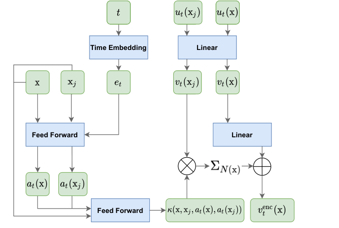
Since the timestamps of input observations are usually fixed, we attempt to model the spatial dependency at each time in the encoder. In this way, we assume that the underlying PDE is supposed to be of the Eq. 2 formulation. Therefore, the encoder of history observations of our model can be chosen as neural-operators-based in Sec. 2.2, whose architecture at a single timestamp is given in Fig. 2.
Solution representation function.
For an observed quantity , we first lift into a higher dimensional representation space with a linear transformation to increase expressiveness, which can be written as , where is defined as representation function. We assume that there exists a true solution representation function in the function space , and we aim to use for approximating it after the mapping of the encoders based on learned operator.
Graph kernel operator.
To encode the history observations into representation space, we use an operator to update to approximate the true solution representation function. We follow kernel operators (Li et al. 2020b; Li et al. 2020a) for parametric PDEs, which is inspired by the solution of uniformly elliptic operator and empirically proved discretization-invariant, to model the action of the integral operator written as
| (4) |
where is a Newtonian potential and is an operator defined by appropriate sums and compositions of the modified trace and co-normal derivative operators (Sauter & Schwab 2011). Lending the Eq. 4 representing an integral operator as iterative architecture, it defines the operator as
| (5) |
where with learnable parameters is the kernel function taking spatial locations , and values of parametric function , as its inputs. As such, the corresponding update approximation which mimics the message passing neural network (Gilmer et al. 2017) is obtained by
| (6) | ||||
where is learnable weights, and is the neighborhood of , which is established by an -ball algorithm (See Appendix A.2.). In specific, we formulate as a feed-forward neural network. By using the proposed multipole graph kernel network, the updating steps are able to capture the long-range spatial dependency between points (Ying et al. 2004; Li et al. 2020a) as well as handle the signals with spatially-irregular distribution. The proposed encoder allows spatially-inductive and temporally-irregularly forecasting: When an observation on an unseen spatial point is obtained, the can be inductively obtained according to Eq. 6 as long as its neighborhood is known. Moreover, for any input , we can always obtain regardless of non-uniform intervals between timestamps.
Parametric function formulation.
For classical PDE models which the kernel operators try to solve, the parametric functions are known. In contrast, the parametric functions are unknown in spatio-temporal forecasting tasks. Thus, we need to approximate parameterized by timestamps and taking location as its input. We first employ trigonometric transformation based on positional encodings used in transformer language models (Vaswani et al. 2017) to embed timestamps into -dimensional space.
| (7) |
where are learnable parameters, and can be a vector containing time features, such as year, month, day and hour. Then, the parametric function is formulated as a feed-forward network taking the concatenation of time embeddings and locations as inputs, i.e. .
3.2 Deep Operator Decoder
In the decoder which is used to generate future predictions given the past representation functions, the values of physical quantities of ground-truth are not given in the prediction process. Therefore, we cannot firstly lift into the representation space for updating. To address it, combined Eq. 1 and Eq. 2, we write the PDE as
| (8) |
which implies . Let , where is the intergal operator, and the construction of is shown in Fig. 3.
Inspired by this, we try to use to approximate , to obtain the representation function solution as
Universal approximation for operator.
Following the Universal Operators in Sec. 2.2, we formulate according to the theorem below.
Theorem 1.
(Universal Approximation Theorem for Operator) (Chen & Chen 1995) Suppose that is a continuous non-polynomial function, is a Banach Space, are two compact sets in and , respectively,
is a compact set in , and is a nonlinear continuous operator, which maps into .
For any , there are positive integers , constants , , , such that
| (9) |
where
holds for all and .

This approximation theorem indicates the potential application of neural networks to learn nonlinear operators from data. Thereby, we let , and . For each future timestamp for prediction, we write its representation solution function as
| (10) | ||||
where , and is the -th component of . Following DeepONet (Lu et al. 2021), we first put the target points into a feed-forward network called Trunk net,
| (11) |
and put all the obtained past representations into the other network called Branch net, as
| (12) |
By multiplying the two outputs of and with a linear transformation whose parameter is stacked after, we obtain the representation function for prediction.
Revised flexible decoder.
The construction of the Branch-Trunk decoder according to Eq. 10 is time-continuous, so it is able to solve the temporally-irregular forecasting theoretically. However, this establishment does not allow inductive forecasting. The reason for it is that:
When a sequence of observations on an unseen spatial point is obtained, the Branch Net in Eq. 12 of the decoder does not permit which is inductively obtained by the encoder to be added to to compute , because the number of parameter for index is fixed as , which is inextensible.
To address it, we revise the Branch net as
| (13) | ||||
We use ‘’ to denote the revised Branch net, which means that the representation functions are updated by aggregating messages from their neighbors’ previous representation functions, where the message-passing weights are inductively obtained by a feed-forward network with relative spatial location and time as inputs. Fig. 4 gives the workflows of our decoder model. In this way, when a sequence of history observations is added, the Branch’s output can still be flexibly obtained as long as the neighborhood is known.
In addition, an auxiliary advantage brought by Eq. 13 is that the potential explosion of model’s parameter number can be avoided. In Eq. 12, when the number of observed points are large, the computational complexity may explore. As increases by 1, the parameter number will increase by , complexity of which may be unaffordable. The revised decoder’s parameter number will not change as the number of spatial sample points increases.
3.3 Loss function
For training, after getting as the values of representation function obtained by encoder, and as the values of representation function obtained by decoder, where are the spatial locations of sample points as shown in Sec. 2.3, we use a linear projector to map them back to , and use mean absolute error (MAE) to construct the loss function, which reads
| (14) | ||||
where the first term we call the reconstruction loss, to restrict the encoder and projector to preserve information from inputs, with ‘the weight of reconstruction loss’, and the second term we call the prediction loss, to evaluate the prediction performance of the model.
4 Related Works
Graph Spatio-temporal networks.
Spatio-temporal forecasting networks are mostly graph-based thanks to their ability to learn representations of spatially-irregular distributed signals, such as traffic flows recorded by sensors (Yu et al. 2018; Li et al. 2018; Guo et al. 2019b; Bai et al. 2020; Zhao et al. 2020; Li et al. 2021a). These works usually regard signals’ location as nodes, and establish graphs to describe the nodes’ dependency according to their spatial distance. Also, some works learn the adjacency relations of nodes without the prior graph structure, by using attention mechanisms (Yu et al. 2018; Li et al. 2018; Zhao et al. 2020), graph structure learning techniques (Shang et al. 2021), node embeddings (Bai et al. 2020) and so on. However, these methods are constructed for transductive tasks on discrete nodes. Recently, a spatio-temporal meteorological forecasting methods for physical quantities located on continuous space (earth sphere) is proposed (Lin et al. 2021), but it still aims to ‘fit’ the signals on discrete nodes. In comparison, our model aims to both handle irregularly distributied signals and allow spatially-inductive forecasting by employing multipole graph neural operators (Li et al. 2020a).
PDE-driven spatio-temporal networks.
An increasing number of works combining spatio-temporal networks with differential equations have been produced in recent years. A series of them are established for data with regular grids, such as videos (Guen & Thome 2020; Donà et al. 2021). These methods are usually constructed on (2D-image-)convolution neural networks as the basic architecture of spatial encoders, while our model aims to handle spatially-irregular distributed points, and thus is graph-based. Another stream of PDE-driven networks follow Neural ODE (Chen et al. 2019) for modeling dynamical systems (Çağatay Yıldız et al. 2019; Rubanova et al. 2019). Because of the high computational cost of integral estimation and backward propagation, these models are not feasible for long-term forecasting. We also establish a version of ODE-based model (Appendix B.) and conduct experiment illustrating its infeasible time cost.
Neural operators.
A line of neural networks have been designed to model one specific instance of the PDEs (E & Yu 2017; Bar & Sochen 2019; Smith et al. 2020; Pan & Duraisamy 2020; Raissi et al. 2020) with prior physical knowledge. For example, structural priors and constraints are combined for fluid prediction (Tompson et al. 2017; Raissi et al. 2020), and Hamiltonian mechanics are used to construct non-regression losses (Greydanus et al. 2019; Chen et al. 2020; Toth et al. 2020) to learn basic laws of physics. In contrast, our model aims to be applicable to general spatio-temporal forecasting. Thus, we turn to neural operators (Lu et al. 2021; Bhattacharya et al. 2021; Li et al. 2020a; Li et al. 2021b; Nelsen & Stuart 2021) for solutions, which require no knowledge of the underlying PDE, only data. Besides, their learned network parameters can be generalized with different discretizations of points. In this way, we conjecture the operator can capture the implicit mechanisms of the dynamics, and thus employ it as the spatial fundamental modules of our model.
5 Experiments
In the experiment part, we aim to figure out the following three questions:
- Q.1
How the proposed STONet performs: Does it achieve improved performance on forecasting tasks of continuous spatial domain, compared with other graph-based spatio-temporal neural networks?
- Q.2
Whether STONet allows spatially-inductive forecasting: Does the trained model achieve comparable accuracy of prediction on unseen spatial points, given their previous observations?
- Q.3
Whether STONet allows temporally-irregular forecasting: Does the model give accurate predictions, even when the labels of future predictions are sampled irregularly, or missing with a ratio?
5.1 Experiment Setup
Protocol.
Because our method is graph-based to handle the spatially-irregular signals or physical quantities, we choose 8 methods which are all graph-based spatio-temporal models for performance comparison. Table. 1 and Appendix C.1. give descriptions of the methods, where ‘Spatial’ and ‘Temporal’ represent the modules to capture spatial dependency and temporal dynamics. Our conclusion is based on the implementation of Torch-Geomtemp (Rozemberczki et al. 2021) and each methods’ open source code. Three widely used metrics - Mean Absolute Error (MAE), Root Mean Square Error (RMSE), and Mean Absolute Percentage Error (MAPE) are deployed to measure the performance. The reported mean and standard deviation of metrics are obtain through 5 independent experiments with different random seeds. All the models for comparison are trained with target function of MAE and optimized by Adam optimizer. The hyper-parameters are chosen through a carefully tuning on the validation set. In implementation, we stack several decoders for different terms of forecasting in STONet as analyzed in Sec. 5.5 and Appendix C.5.
| Methods | Spatial | Temporal |
|---|---|---|
| TGCN (Zhao et al. 2020) | Vanilla GCN (Kipf & Welling 2017) | GRU |
| STGCN (Yu et al. 2018) | Vanilla GCN (Kipf & Welling 2017) | 1D Conv |
| MSTGCN (Guo et al. 2019a) | ChebConv (Defferrard et al. 2017) | 1D Conv |
| ASTGCN (Guo et al. 2019a) | GAT (Veličković et al. 2018) | Attention |
| GCGRU (Seo et al. 2016) | ChebConv (Defferrard et al. 2017) | GRU |
| DCRNN (Li et al. 2018) | DiffConv (Atwood & Towsley 2016) | GRU |
| AGCRN (Bai et al. 2020) | Node Similarity (Bai et al. 2020) | GRU |
| CLCRN (Lin et al. 2021) | CondLocalConv (Lin et al. 2021) | GRU |
Dataset.
We conduct an evaluation on 6 datasets, whose forecasting target signals are all spatially-continuous physical quantities, including Wave (Saha et al. 2021), Solar energy (Lai et al. 2018), Temperature, Humidity, Cloud cover and Wind component (Rasp et al. 2020). All the evaluation tasks are 12-to-12 auto-regressive forecasting, where the input and forecasting sequence length are all set as 12. The spatial domain includes both 2D plane and 2D sphere (earth’s surface). Dataset descriptions are shown in Table. 2. For CLCRN (Lin et al. 2021), it is established for dataset whose spatial domain is sphere, so we do not compare its performance on planar dataset. To differentiate from the time point, we call the fixed spatial points as nodes, because all the methods are graph-based.
| Datasets | Wave | Solar Energy | Temperature |
|---|---|---|---|
| Spatial domain | 2D plane | 2D plane | 2D sphere |
| Dimension | 1 | 1 | 1 |
| # of nodes | 512 | 137 | 2048 |
| Granularity | 0.001s | 5 min | 1h |
| Datasets | Humidity | Cloud cover | Wind component |
| Spatial domain | 2D sphere | 2D sphere | 2D sphere |
| Dimension | 1 | 1 | 2 |
| # of nodes | 2048 | 2048 | 2048 |
| Granularity | 1h | 1h | 1h |
5.2 Performance Comparison
We first conduct experiments on the datasets with 8 baselines and our STONet. Because MAPE is of great difference among methods and hard to agree on an order of magnitude due to its incompatible units, we show it in Appendix C.2.
| MAE | RMSE | MAE | RMSE | MAE | RMSE | |
| Wave () | Solar Energy (MW) | Temperature (K) | ||||
| TGCN | 3.7619±0.0144 | 5.8999±0.0485 | 2.0036±0.0423 | 4.6218±0.3820 | 3.8638±0.0970 | 5.8554±0.1432 |
| STGCN | 4.1202±0.1800 | 6.4805±0.4165 | 1.4048±0.0184 | 4.1451±0.0249 | 4.3525±1.0442 | 6.8600±1.1233 |
| MSTGCN | 6.0639±0.2664 | 7.8891±0.5628 | 1.9224±0.0251 | 4.0406±0.0471 | 1.2199±0.0058 | 1.9203±0.0093 |
| ASTGCN | 5.3150±0.2012 | 7.1699±0.2045 | 1.9834±0.0054 | 4.1312±0.0095 | 1.4896±0.0130 | 2.4622±0.0023 |
| GCGRU | 3.5617±0.4817 | 5.6927±0.4181 | 1.0661±0.0867 | 2.6303±0.1197 | 1.3256±0.1499 | 2.1721±0.1945 |
| DCRNN | 3.7338±0.1167 | 5.8157±0.0859 | 1.1031±0.1140 | 2.7474±0.2229 | 1.3232±0.0864 | 2.1874±0.1227 |
| AGCRN | 4.2048±0.1161 | 6.1559±0.0776 | 1.1845±0.0902 | 2.6823±0.1261 | 1.2551±0.0080 | 1.9314±0.0219 |
| CLCRN | - | - | - | - | 1.1688±0.0457 | 1.8825±0.1509 |
| STONet | 3.1959±0.0722 | 5.2201±0.0743 | 0.8699±0.0399 | 2.1533±0.0563 | 0.8972±0.0230 | 1.4963±0.0422 |
| Improvements | 10.2703% | 8.3019% | 18.4035% | 18.1348% | 23.2375% | 20.5153% |
| Humidity () | Cloud Cover () | Wind Component () | ||||
| TGCN | 1.4700±0.0295 | 2.1066±0.0551 | 2.3934±0.0216 | 3.6512±0.0223 | 4.1747±0.0324 | 5.6730±0.0412 |
| STGCN | 0.7975±0.2378 | 1.1109±0.2913 | 2.0197±0.0392 | 2.9542±0.0542 | 3.6477±0.0000 | 4.8146±0.0003 |
| MSTGCN | 0.6093±0.0012 | 0.8684±0.0019 | 1.8732±0.0010 | 2.8629±0.0073 | 1.9440±0.0150 | 2.9111±0.0292 |
| ASTGCN | 0.7288±0.0229 | 1.0471±0.0402 | 1.9936±0.0002 | 2.9576±0.0007 | 2.0889±0.0006 | 3.1356±0.0012 |
| GCGRU | 0.5007±0.0002 | 0.7891±0.0006 | 1.5925±0.0023 | 2.5576±0.0116 | 1.4116±0.0057 | 2.2931±0.0047 |
| DCRNN | 0.5046±0.0011 | 0.7956±0.0033 | 1.5938±0.0021 | 2.5412±0.0044 | 1.4321±0.0019 | 2.3364±0.0055 |
| AGCRN | 0.5759±0.1632 | 0.8549±0.2025 | 1.7501±0.1467 | 2.7585±0.1694 | 2.4194±0.1149 | 3.4171±0.1127 |
| CLCRN | 0.4531±0.0065 | 0.7078±0.0146 | 1.4906±0.0037 | 2.4559±0.0027 | 1.3260±0.0483 | 2.1292±0.0733 |
| STONet | 0.4273±0.0256 | 0.6584±0.0287 | 1.4933±0.0030 | 2.4142±0.0016 | 1.2192±0.0064 | 1.9774±0.0122 |
| Improvements | 5.6841% | 6.9794% | -0.1811% | 1.7794% | 8.0543% | 7.1294% |
From Table. 3, it can be concluded that
- •
Due to the high expressivity of STONet, it outperforms other models for comparison with a large margin on all but the smallest of the benchmark datasets such as Cloud Cover.
- •
Because most of the compared methods are established for traffic forecasting on discrete nodes, they show a decrease in performance for continuous physical quantity forecasting tasks. The difference between two tasks is analyzed in previous works (Lin et al. 2021).
5.3 Spatially Inductive Evaluation
The second part is to figure out Q.2 : whether the proposed STONet allows spatially-inductive forecasting. We preprocess the datasets to ensure that there are unseen the spatial nodes in the datasets for models to be trained with. For example, for the four weather datasets, we first downsample the resolution to , with nodes used for training, and randomly choose another different nodes for inductive evaluation. Other details on preprocessing datasets for this task are described in Appendix C.3.


Our results of performance on original nodes (for transductive forecasting) and unseen nodes (for inductive forecasting) are shown in Table. 4, where ‘Deviation’ is calculated by . Fig. 5 shows the performance of inductive tasks on unseen nodes with different ratios, where , on several datasets. Results on other datasets are in Appendix C.3. We conclude that
| Metric | Tasks | Wave | Solar Energy | Temperature |
|---|---|---|---|---|
| MAE | Trans. | 3.1959±0.0722 | 1.1448±0.0206 | 0.9344±0.0252 |
| Induc. | 3.1719±0.3624 | 1.1799±0.0373 | 0.9638±0.0371 | |
| RMSE | Trans. | 5.2586±0.0743 | 2.4654±0.0454 | 1.5250±0.0455 |
| Induc. | 5.3794±0.2933 | 2.5028±0.0427 | 1.5631±0.0594 | |
| Deviation | -0.7509% | +3.0660% | +3.1464% | |
| Metric | Tasks | Humidity | Cloud Cover | Wind Component |
| MAE | Trans. | 0.4678±0.0167 | 1.5874±0.0028 | 1.3124±0.0149 |
| Induc. | 0.4847±0.0248 | 1.6024±0.0101 | 1.3330±0.0154 | |
| RMSE | Trans. | 0.7075±0.0150 | 2.5223±0.0039 | 2.1588±0.0375 |
| Induc. | 0.7398±0.0132 | 2.5213±0.0183 | 2.1459±0.0462 | |
| Deviation | +3.6082% | +0.9449% | +1.5696% |
- •
The overall performance on transductive tasks shows decrease except in Wave, because downsampling is conducted in the other five datasets, causing the loss of spatial information.
- •
The evaluation on unseen nodes usually shows a tiny decrease compared with the nodes for training, but still achieves a competitive accuracy with the ‘Deviation’ less than .
- •
As the ratio of unseen points increases, the performance on them usually shows a trend of decrease with some fluctuation. An explanation of it is that the message-passing patterns of STONet entangle intricately, and could possibly be disturbed when a large number of unseen nodes are included for forecasting.
To sum up, empirical studies illustrate that the inductive forecasting task can be well-solved by our model when the number of unseen nodes is not extremely large, since the deviation is smaller than in different s.
5.4 Temporally Irregular Evaluation
To demonstrate that our model can solve the Q.3, we conduct experiments in one of the temporally-irregular forecasting scenarios – data with missing values, since all the evaluated datasets are all uniformly sampled in temporal domains. In detail, the previous setting is all based on a -to- forecasting task, where , while in this part, we randomly remove labels of different sequences of data at different timestamps with a ratio, leading to the non-uniformity of time-interval. We set , where . For example, if we randomly remove spatial snapshots at timestamps, we think that it is equivalent to the missing data scenario where the missing ratio equals , and .


Fig. 6 shows the performance change of different . Intuitively, when the is extremely small, e.g. and missing ratio equals , the performance demonstrates a dramatical decrease, due to a massive loss of supervised labels. In comparison, when the missing ratio is small, e.g. , the performance is comparable. Therefore, even if STONet has the ability to handle the temporally-irregular forecasting tasks, a large ratio of missing data in the temporal domain compromises the model performance.
5.5 Further Ablation Study
Several hyper-parameters affect the model performance, and in this part we try to explore their impacts. First, we aim to figure out how the ‘embedding size’ i.e. , and the ‘layer number’ determine the expressivity of the model. Second, as demonstrated in (Li et al. 2020a), the multi-leveled graphs in multipole graph neural network encoder help to increase the accuracy, because it enables each node to aggregate messages from farther nodes in spatial domains. Thus, we attempt to figure out its effects. Note that when the ‘number of levels’ of multipole graphs equals , the graph kernel encoder in STONet is the same as proposed in (Simonovsky & Komodakis 2017). Finally, we conduct analysis on , the ‘weight of the reconstruction loss’. We give results on Solar Energy and Temperature, and the results on other datasets are shown in Appendix C.5.


| Datasets | Solar Energy | Temperature | ||
| # of levels | MAE | RMSE | MAE | RMSE |
| 1 | 1.0630±0.0359 | 2.5188±0.0490 | 0.8917±0.0164 | 1.4825±0.0423 |
| 2 | 0.9729±0.2378 | 2.3364±0.2913 | 0.8718±0.0302 | 1.4311±0.0571 |
| 3 | 0.8699±0.0207 | 2.1533±0.0305 | 0.8972±0.0230 | 1.4963±0.0422 |
| Datasets | Solar Energy | Temperature | ||
| loss weight | MAE | RMSE | MAE | RMSE |
| 0.0 | 0.9195±0.0102 | 2.1677±0.0209 | 0.8845±0.0196 | 1.4837±0.0313 |
| 0.5 | 0.8699±0.0399 | 2.1533±0.0563 | 0.8972±0.0230 | 1.4963±0.0422 |
| 1.0 | 0.9159±0.0430 | 2.1724±0.0625 | 0.9692±0.0216 | 1.5880±0.0392 |
6 Conclusion
An operator-driven spatio-temporal forecasting network is proposed, with its encoder based on graph kernel operator and decoder based on universal operator. Experiments show that it achieves improved performance in continuous physical quantities forecasting on spatial points of spatially-irregular distribution , and allows both spatially-inductive and temporally-irregular forecasting.
References
- Antman (2005) Antman, S. S. Nonlinear problems of elasticity. 2005.
- Atwood & Towsley (2016) Atwood, J. and Towsley, D. Diffusion-convolutional neural networks, 2016.
- Bai et al. (2020) Bai, L., Yao, L., Li, C., Wang, X., and Wang, C. Adaptive graph convolutional recurrent network for traffic forecasting, 2020.
- Bar & Sochen (2019) Bar, L. and Sochen, N. Unsupervised deep learning algorithm for pde-based forward and inverse problems, 2019.
- BearM & Corapcioglu (2012) BearM, J. and Corapcioglu, Y. Physics-informed probabilistic learning of linear embeddings of nonlinear dynamics with guaranteed stability. 2012.
- Bhattacharya et al. (2021) Bhattacharya, K., Hosseini, B., Kovachki, N. B., and Stuart, A. M. Model reduction and neural networks for parametric pdes, 2021.
- Chen et al. (2019) Chen, R. T. Q., Rubanova, Y., Bettencourt, J., and Duvenaud, D. Neural ordinary differential equations, 2019.
- Chen & Chen (1995) Chen, T. and Chen, H. Universal approximation to nonlinear operators by neural networks with arbitrary activation functions and its application to dynamical systems. IEEE Transactions on Neural Networks, 6(4):911–917, 1995. doi: 10.1109/72.392253.
- Chen et al. (2020) Chen, Z., Zhang, J., Arjovsky, M., and Bottou, L. Symplectic recurrent neural networks, 2020.
- Defferrard et al. (2017) Defferrard, M., Bresson, X., and Vandergheynst, P. Convolutional neural networks on graphs with fast localized spectral filtering, 2017.
- Donà et al. (2021) Donà, J., Franceschi, J.-Y., Lamprier, S., and Gallinari, P. Pde-driven spatiotemporal disentanglement, 2021.
- E & Yu (2017) E, W. and Yu, B. The deep ritz method: A deep learning-based numerical algorithm for solving variational problems, 2017.
- Gilmer et al. (2017) Gilmer, J., Schoenholz, S. S., Riley, P. F., Vinyals, O., and Dahl, G. E. Neural message passing for quantum chemistry, 2017.
- Greenfeld et al. (2019) Greenfeld, D., Galun, M., Kimmel, R., Yavneh, I., and Basri, R. Learning to optimize multigrid pde solvers, 2019.
- Greydanus et al. (2019) Greydanus, S., Dzamba, M., and Yosinski, J. Hamiltonian neural networks, 2019.
- Guen & Thome (2020) Guen, V. L. and Thome, N. Disentangling physical dynamics from unknown factors for unsupervised video prediction, 2020.
- Guo et al. (2019a) Guo, S., Lin, Y., Feng, N., Song, C., and Wan, H. Attention based spatial-temporal graph convolutional networks for traffic flow forecasting. Proceedings of the AAAI Conference on Artificial Intelligence, 33(01):922–929, Jul. 2019a. doi: 10.1609/aaai.v33i01.3301922. URL https://ojs.aaai.org/index.php/AAAI/article/view/3881.
- Guo et al. (2019b) Guo, S., Lin, Y., Feng, N., Song, C., and Wan, H. Attention based spatial-temporal graph convolutional networks for traffic flow forecasting. In Proceedings of the AAAI Conference on Artificial Intelligence, volume 33, pp. 922–929, 2019b.
- Jiang et al. (2020) Jiang, C. M., Esmaeilzadeh, S., Azizzadenesheli, K., Kashinath, K., Mustafa, M., Tchelepi, H. A., Marcus, P., Prabhat, and Anandkumar, A. Meshfreeflownet: A physics-constrained deep continuous space-time super-resolution framework, 2020.
- Kipf & Welling (2017) Kipf, T. N. and Welling, M. Semi-supervised classification with graph convolutional networks, 2017.
- Kochkov et al. (2021) Kochkov, D., Smith, J. A., Alieva, A., Wang, Q., Brenner, M. P., and Hoyer, S. Machine learning accelerated computational fluid dynamics, 2021.
- Lai et al. (2018) Lai, G., Chang, W.-C., Yang, Y., and Liu, H. Modeling long- and short-term temporal patterns with deep neural networks, 2018.
- Li et al. (2021a) Li, F., Feng, J., Yan, H., Jin, G., Jin, D., and Li, Y. Dynamic graph convolutional recurrent network for traffic prediction: Benchmark and solution, 2021a.
- Li et al. (2018) Li, Y., Yu, R., Shahabi, C., and Liu, Y. Diffusion convolutional recurrent neural network: Data-driven traffic forecasting, 2018.
- Li et al. (2020a) Li, Z., Kovachki, N., Azizzadenesheli, K., Liu, B., Bhattacharya, K., Stuart, A., and Anandkumar, A. Multipole graph neural operator for parametric partial differential equations, 2020a.
- Li et al. (2020b) Li, Z., Kovachki, N., Azizzadenesheli, K., Liu, B., Bhattacharya, K., Stuart, A., and Anandkumar, A. Neural operator: Graph kernel network for partial differential equations, 2020b.
- Li et al. (2021b) Li, Z., Kovachki, N., Azizzadenesheli, K., Liu, B., Bhattacharya, K., Stuart, A., and Anandkumar, A. Fundamentals of transport phenomena in porous media, 2021b.
- Lin et al. (2021) Lin, H., Gao, Z., Xu, Y., Wu, L., Li, L., and Li, S. Z. Conditional local convolution for spatio-temporal meteorological forecasting, 2021.
- Lu et al. (2021) Lu, L., Jin, P., Pang, G., Zhang, Z., and Karniadakis, G. E. Learning nonlinear operators via deeponet based on the universal approximation theorem of operators. Nature Machine Intelligence, 3:218–229, 2021.
- Nelsen & Stuart (2021) Nelsen, N. H. and Stuart, A. M. The random feature model for input-output maps between banach spaces, 2021.
- Pan & Duraisamy (2020) Pan, S. and Duraisamy, K. Physics-informed probabilistic learning of linear embeddings of nonlinear dynamics with guaranteed stability. SIAM Journal on Applied Dynamical Systems, 19(1):480–509, Jan 2020. ISSN 1536-0040. doi: 10.1137/19m1267246. URL http://dx.doi.org/10.1137/19M1267246.
- Raissi et al. (2019) Raissi, M., Perdikaris, P., and Karniadakis, G. Physics-informed neural networks: A deep learning framework for solving forward and inverse problems involving nonlinear partial differential equations. Journal of Computational Physics, 378:686–707, 2019. ISSN 0021-9991. doi: https://doi.org/10.1016/j.jcp.2018.10.045. URL https://www.sciencedirect.com/science/article/pii/S0021999118307125.
- Raissi et al. (2020) Raissi, M., Yazdani, A., and Karniadakis, G. E. Hidden fluid mechanics: Learning velocity and pressure fields from flow visualizations. Science, 367(6481):1026–1030, 2020.
- Rasp et al. (2020) Rasp, S., Dueben, P. D., Scher, S., Weyn, J. A., Mouatadid, S., and Thuerey, N. Weatherbench: A benchmark dataset for data-driven weather forecasting, 2020.
- Rozemberczki et al. (2021) Rozemberczki, B., Scherer, P., He, Y., Panagopoulos, G., Riedel, A., Astefanoaei, M., Kiss, O., Beres, F., Lopez, G., Collignon, N., and Sarkar, R. Pytorch geometric temporal: Spatiotemporal signal processing with neural machine learning models, 2021.
- Rubanova et al. (2019) Rubanova, Y., Chen, R. T. Q., and Duvenaud, D. Latent odes for irregularly-sampled time series, 2019.
- Saha et al. (2021) Saha, P., Dash, S., and Mukhopadhyay, S. Physics-incorporated convolutional recurrent neural networks for source identification and forecasting of dynamical systems, 2021.
- Sauter & Schwab (2011) Sauter, S. A. and Schwab, C. Boundary element methods. 2011.
- Seo et al. (2016) Seo, Y., Defferrard, M., Vandergheynst, P., and Bresson, X. Structured sequence modeling with graph convolutional recurrent networks, 2016.
- Shang et al. (2021) Shang, C., Chen, J., and Bi, J. Discrete graph structure learning for forecasting multiple time series, 2021.
- Shi et al. (2015) Shi, X., Chen, Z., Wang, H., Yeung, D.-Y., kin Wong, W., and chun Woo, W. Convolutional lstm network: A machine learning approach for precipitation nowcasting, 2015.
- Simonovsky & Komodakis (2017) Simonovsky, M. and Komodakis, N. Dynamic edge-conditioned filters in convolutional neural networks on graphs, 2017.
- Smith et al. (2020) Smith, J. D., Azizzadenesheli, K., and Ross, Z. E. Eikonet: Solving the eikonal equation with deep neural networks, 2020.
- Tompson et al. (2017) Tompson, J., Schlachter, K., Sprechmann, P., and Perlin, K. Accelerating eulerian fluid simulation with convolutional networks, 2017.
- Toth et al. (2020) Toth, P., Rezende, D. J., Jaegle, A., Racanière, S., Botev, A., and Higgins, I. Hamiltonian generative networks, 2020.
- Vaswani et al. (2017) Vaswani, A., Shazeer, N., Parmar, N., Uszkoreit, J., Jones, L., Gomez, A. N., Kaiser, L., and Polosukhin, I. Attention is all you need, 2017.
- Veličković et al. (2018) Veličković, P., Cucurull, G., Casanova, A., Romero, A., Liò, P., and Bengio, Y. Graph attention networks, 2018.
- Ying et al. (2004) Ying, L., Biros, G., and Zorin, D. A kernel-independent adaptive fast multipole algorithm in two and three dimensions. Journal of Computational Physics, 196(2):591–626, 2004. ISSN 0021-9991. doi: https://doi.org/10.1016/j.jcp.2003.11.021. URL https://www.sciencedirect.com/science/article/pii/S0021999103006090.
- Yu et al. (2018) Yu, B., Yin, H., and Zhu, Z. Spatio-temporal graph convolutional networks: A deep learning framework for traffic forecasting. Proceedings of the Twenty-Seventh International Joint Conference on Artificial Intelligence, Jul 2018. doi: 10.24963/ijcai.2018/505. URL http://dx.doi.org/10.24963/ijcai.2018/505.
- Zhao et al. (2020) Zhao, L., Song, Y., Zhang, C., Liu, Y., Wang, P., Lin, T., Deng, M., and Li, H. T-gcn: A temporal graph convolutional network for traffic prediction. IEEE Transactions on Intelligent Transportation Systems, 21(9):3848–3858, Sep 2020. ISSN 1558-0016. doi: 10.1109/tits.2019.2935152. URL http://dx.doi.org/10.1109/TITS.2019.2935152.
- Çağatay Yıldız et al. (2019) Çağatay Yıldız, Heinonen, M., and Lähdesmäki, H. Ode2vae: Deep generative second order odes with bayesian neural networks, 2019.
A. Notation and Method Supplementary
A.1. Glossary of notations
| Symbol | Used for |
|---|---|
| Time or timestamps. | |
| Spatial locations. | |
| Spatial locations which are unseen by models during training. | |
| Physical quantities or continuous signals with spatial location and time as input . | |
| neighborhood of . | |
| Mapping of historical observations into future predictions. | |
| Parametric function in parametric PDEs. | |
| Differential operator in parametric PDEs. | |
| Operator for solving the parametric PDEs, mapping paramteric function to solution function. | |
| Operator for approximating true operators in the parametric PDEs. | |
| Kernel operator as an instance of for solving the parametric PDEs. | |
| Operator of groundtruth. | |
| Universal Operator to approximate the operator of groundtruth. | |
| Parameters in universal operator. | |
| Solution representation function obtained by encoders. | |
| Solution representation function obtained by decoders. | |
| Projector to map into . | |
| Projector to map back into . |
A.2. Multipole graph construction
Neighborhood construction.
The neighborhood system is constructed by -ball, which can be written as for point ,
| (15) |
is the distance between point and . In the planar dataset, the is calculated by
| (16) |
while in the sphere dataset, the distance term is calculated by
| (17) |
Multipole graph kernel algorithm.
The multipole method is to use a series of sparse and low-rank matrix to approximate the true kernel matrix. The true kernel matrix is decomposed into a hierarchy of low-rank structures. First, all the spatial points are randomly divided into levels, and for each level , the graph message passing is firstly operated inter-level, as
| (18) |
Then, the low-level points’ representation will be used to update the high-level one, as
| (19) |
and the high-level points’ representation will be also used to update the points of low level reversely, as
| (20) |
It can be regarded as decomposing the kernel with a series of low-rank matrix by recursively applying the three steps. And for each point, it can aggregate messages from neighbors of different levels, and thus the recursive structure of the algorithm can allow each point to be affected farther points, although it consumes more time.
B. A ODE-based Decoder
We establish another decoder based on Neural ODE (Chen et al. 2019). The ODE-based decoder is constructed by
| (21) |
In this way, we first use a universal operator to approximate , and then use the Neural ODE, reads
For our model aims to handle the long-term prediction, the ‘backward’ process is extremely slow, thus we regard it as computational infeasible. Table 7 gives the comparison on ODE-based decoder and non-ODE-based decoder on the dataset of Solar Energy and Humidity on one epoch, and the performance comparison. Because the ODE-based decoder is extremely time-consuming, thus we did not conduct experiments on other datasets to show its effectiveness. It shows that our model is superior to the ODE-based one in terms of both computational efficiency and prediction accuracy, because the over-fitting effects are extremely obvious in ODE-based one.
| Datasets | Humidity | ||||
| Decoder Type | set | MAE | RMSE | Memory | Time |
| ODE-based | train | 3.1491±0.4533 | 7.1483±0.0991 | 13641MB | |
| test | 12.083±6.2098 | 17.2462±9.5624 | |||
| Non-ODE-based | test | 0.8699±0.0399 | 2.1533±0.0563 | 16163MB | |
| Datasets | Solar Energy | ||||
| Decoder Type | set | MAE | RMSE | Memory | Time |
| ODE-based | train | 0.6466±0.0610 | 0.8975±0.1312 | 22957MB | |
| test | 2.0103±0.4933 | 2.1439±0.3534 | |||
| Non-ODE-based | test | 0.4273±0.0256 | 0.6584±0.0287 | 25183MB | |


C. Experiment Supplementary
C.1. Method description
(1) TGCN is proposed for traffic forecasting, with the traffic sensors’ graph constructed according to the road distance. The spatial convolution is based on Vanilla GCN, which uses the normed Laplacian matrix as the aggregation operator, and its temporal dynamics is modeled by GRU.
(2) STGCN is also proposed for traffic forecasting. Different from TGCN, its temporal dynamics is modeled by 1DConv.
(3) MSTGCN which is established for traffic forecasting, its spatial dependency is captured by ChebConv, which is a higher-order version of Vanilla GCN, approximating the graph spectral filters by Chebshev polynomials.
(4) ASTGCN as a traffic forecasting model, is fully attention based, with spatial dependency captured by graph-attention mechanisms, and temporal dynamics captured by series self-attention.
(5) GCGRU uses high order ChebConv to replace the linear transformation layers in GRU. It is established for many multi-variate time series forecasting tasks.
(6) AGCRN trains the node embeddings, with the product of two node embeddings as their similarity, to adaptively construct the semantic graph as spatial dependency. It is established for many multi-variate time series forecasting tasks, not only limited in traffic forecasting.
(7) CLCRN as a spatio-temporal meteorological forecasting model, employs the conditional local convolution which is established for spherical datasets, and based on the assumption of smoothness of local patterns in weather forecasting. It is the state-of-the-art method for geophysical quantities forecasting.
C.2. Model comparision
Metrics computation.
Let
| (24) | |||
| (25) |
be the ground truth and the predictions obtained by neural networks respectively. The three metrics including MAE, RMSE and MAPE are calculated as
MAPE comparison.
Here we give the metrics of MAPE obtained by different methods, shown in Fig. 8. MAPE metrics is not stable, because there exists a term in the denominator, and thus we do not consider the contributions of terms with ground truth equaling 0. However, for datasets Wave, Solar Energy and Cloud Cover, the minimal is still extremely small, causing the MAPE term extremely large. Therefore, we think the comparison of MAPE on these three datasets are not meaningful.
C.3. Spatially-inductive forecasting
Data preprocess.
The nodes in each dataset need to be re-divided into nodes for training and nodes for inductive evaluation. The detailed processing is
- •
For Wave, The nodes are originally sampled from images, so we randomly choose another nodes to evaluate models’ spatially-inductive forecasting ability.
- •
For Solar Energy: Since it is a dataset with low-resolution, we randomly choose nodes for training, and the rest nodes are used for inductive evaluation.
- •
Four the weather datasets: We first downsample the resolution to , with nodes used for training, and randomly choose another different nodes for inductive evaluation.
Fig. 13 gives further details on spatially-inductive forecasting on all datasets except Solar Energy, because the inductive ratio is always fixed for such a dataset of low spatial resolution. It shows that with the increase of the inductive ‘Ratio’, the prediction accuracy decreases. However, all the deviations are very small and acceptable.
C.4. Temporally-irregular forecasting
Fig. 14 gives further details on temporally-irregular forecasting on all datasets except Solar Energy. As the output timestamps’ labels fed in the model decrease, the predictive performance decrease due to excessive loss of supervised signals and information.
C.5. Ablation Study
For each dataset, we give ablation study on the four hyper-parameters, which are ‘embedding size’, ‘layer number’, ‘level numbers’ and ‘weight of reconstruction loss’. The change of performance with the change of hyper-parameters is shown in Fig. 9, 10, 11 and 12 respectively.


