Lane-Free Crossing of CAVs through Intersections as a Minimum-Time Optimal Control Problem

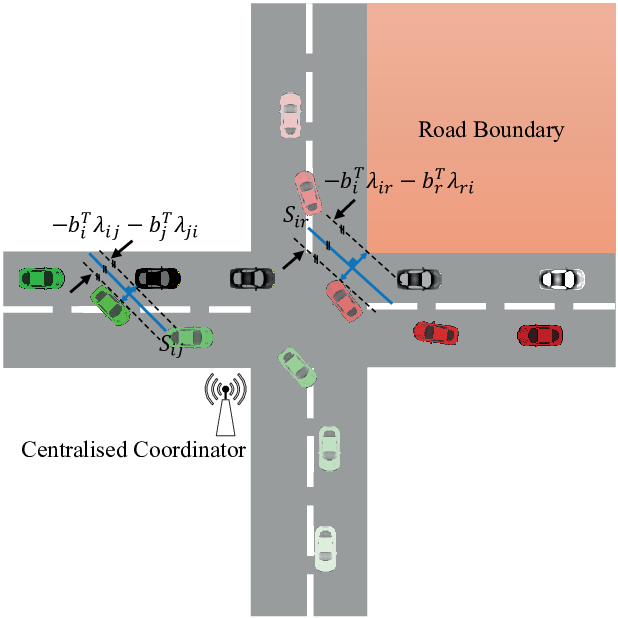
Fig. 1 illustrates an example layout of a lane-free and signal-free intersection. The figure includes three CAVs which are moving from their initial points, depicted with the most solid colour, towards their intended destinations which are with the most transparent colour. The intersection comprises of four approaches, each of them has a separate incoming and outgoing lane. In a lane-free intersection, vehicles can freely change their lanes in favour of faster crossing through the intersection. For instance, Fig. 1 shows the green CAV overtakes the black CAV by using the opposite lane. It is worth noting that the intersection does not have traffic lights because the CAVs can directly communicate their states and intentions. In this study, there is a coordinator that receives all the information from the CAVs and centrally control the vehicles to efficiently and safely cross the intersection. This fully-connected and centralised topology provides the optimal solution as the benchmark for testing any decentralised strategy.

The black and green CAVs also show the collision avoidance. The expression $-b_{i}^{\top}\lambda_{ij}-b_{j}^{\top}\lambda_{ji}$ is the dual representation of the distance between a pair of CAVs whilst $S_{ij}^{*}$ is the separating hyperplane placed between them. Similarly, $-b_{i}^{\top}\lambda_{ir}-b_{r}^{\top}\lambda_{ri}$ is the dual representation of distance between the red CAV and the coloured road boundary whilst $S_{ir}^{*}$ is the separating hyperplane between them. These equations are further explained in section 3.

This study represents the lateral behaviour of a $\text{CAV}_{i},\forall i\in\{1..N\}$ where $N$ is the number of crossing CAVs, with the bicycle model [9]. The bicycle model consists of two degree-of-freedoms (DoFs) which are sideslip angle $\beta_{i}$ and yaw rate $r_{i}$. The model also includes an additional DoF for the longitudinal velocity $V_{i}$. The pose of the $\text{CAV}_{i}$ at each time $t$ with respect to its initial pose is then calculated from these states. The equations of the DoFs along with the pose of $\text{CAV}_{i}$ construct a set of non-linear differential equations as follows:

where $\textbf{x}=[r_{i},\beta_{i},V_{i},x_{i},y_{i},\theta_{i}]^{T}$ and $\textbf{u}=[a_{i},\delta_{i}]^{T}$ are, respectively, the system states and control inputs of $\text{CAV}_{i}$. $a_{i}(t)$ and $\delta_{i}(t)$ are, respectively, the acceleration ($m/s^{2}$) and steering angle ($rad$) of the vehicle. $\textbf{z}_{i}=[x_{i},y_{i},\theta_{i}]^{T}$ refers to the pose of $\text{CAV}_{i}$ in non-inertial reference system. The constants $m$ and $I_{z}$ denote mass ($kg$) and moment of inertia ($kg.m^{2}$) of the vehicle around axis $z$, respectively. $t_{0}$ and $t_{f}$ ($s$) represent the starting and ending time of the crossing. The calculation of vehicle parameters $\tilde{N}_{r}$, $N_{\beta}$, $N_{\delta}$, $\tilde{Y}_{r}$, $Y_{\beta}$ and $Y_{\delta}$ is shown in [9].

To ensure CAVs drive within their dynamic limitations, the following constraints are enforced for each $\text{CAV}_{i}$:

where $\overline{.}$ and $\underline{.}$ are, respectively, the upper and lower boundaries.

Each $\text{CAV}_{i}$ is presented as a rectangular polytope $\zeta_{i}$ at origin where as the intersection of half-space linear inequality $A_{i}X\leq b_{i}$ where $X=[x,y]^{T}$ is a Cartesian point.

Road boundaries are also modelled with convex polytopic sets $O_{r}$ where $r\in\{1..N_{r}\}$ and $N_{r}=4$ denotes the total number of road boundaries for a four-legged intersection.

To avoid collisions between any $\text{CAV}_{i}$ and $\text{CAV}_{j}$ $\forall i\neq j\in\{1..N\}$, their polytopic sets should not intersect, i.e. $\zeta_{i}\cap\zeta_{j}=\emptyset$ where $\zeta_{i}=\{\text{X}\in\mathbb{R}^{2}|A_{i}\text{X}\leq b_{i}\}$ and $\zeta_{j}=\{\text{Y}\in\mathbb{R}^{2}|A_{j}\text{Y}\leq b_{j}\}$. However, this is a non-convex and non-differentiable constraint. To enforce differentiability, $\zeta_{i}\cap\zeta_{j}=\emptyset$ is replaced by the following sufficient condition [16]:

where $d_{min}$ is a minimum safety distance between any pair of CAVs.

It is known that the problem of finding the minimum distance between a polytope $\zeta_{i}$ and another given polytope $\zeta_{j}$ is convex [2]. Therefore the substituting sufficient condition, $dist(\zeta_{i},\zeta_{j})\geq d_{min}$, is convex and since $\zeta_{j}$ is not an empty set, the strong duality holds [16]. This means that the solution of the primal problem $dist(\zeta_{i},\zeta_{j})\geq d_{min}$ is the same as the one of its dual problem which is as follows:

where $\lambda_{ij}$, $\lambda_{ji}$, and $s_{ij}$ are the dual variables. $A_{i}$ and $b_{i}$ represent the $\text{CAV}_{i}$’s polytope at each time step $t$, and are functions of the $\text{CAV}_{i}$’s pose $\textbf{z}_{i}(t)$. The derivation of dual problem (4) from primal problem (3.1) is shown in [4].

Combining (4) with (3.1), (4) can be substituted by $\{\exists\lambda_{ij}\geq 0,\lambda_{ji}\geq 0,s_{ij}:-b_{i}^{\top}\lambda_{ij}-b_{j}^{\top}\lambda_{ji}\geq d_{min},A_{i}^{\top}\lambda_{ij}+s_{ij}=0,A_{j}^{\top}\lambda_{ji}-s_{ij}=0,\left\lVert s_{ij}\right\rVert_{2}\leq 1\}$ because the existence of a feasible solution $\lambda_{ij,feas}$, $\lambda_{ji,feas}$, and $s_{ij,feas}$ where $-b_{i}^{\top}\lambda_{ij,feas}-b_{j}^{\top}\lambda_{ji,feas}\geq d_{min}$ is a sufficient condition to ensure $dist(\zeta_{i},\zeta_{j})\geq d_{min}$, i.e. to avoid collisions [4]. As seen in Fig. 1, $S_{ij}$ is a separating hyperplane between $\text{CAV}_{i}$ and $\text{CAV}_{j}$, and $S_{ij}$ = $S_{ji}$.

Each $\text{CAV}_{i}$ must also avoid all the road boundaries, i.e. $\zeta_{i}\cap O_{r}=\emptyset$ where $\zeta_{i}=\{\text{X}\in\mathbb{R}^{2}|A_{i}\text{X}\leq b_{i}\}$ and $O_{r}=\{\text{Y}\in\mathbb{R}^{2}|A_{r}\text{Y}\leq b_{r}\}$. Similar to section 3.1, $\zeta_{i}\cap O_{r}=\emptyset$ is replaced by the following sufficient condition:

where $d_{rmin}$ is the minimum safety distance between CAVs and road boundaries.

The dual problem of (3.2) is then substituted with the sufficient condition $\{\exists\lambda_{ir}\geq 0,\lambda_{ri}\geq 0,s_{ir}:-b_{i}^{\top}\lambda_{ir}-b_{r}^{\top}\lambda_{ri}\geq d_{rmin},A_{i}^{\top}\lambda_{ir}+s_{ir}=0,A_{j}^{\top}\lambda_{ri}-s_{ir}=0,\left\lVert s_{ir}\right\rVert_{2}\leq 1\}$ where $\lambda_{ir},\lambda_{ri}$, and $s_{ir}$ are the dual variables. $S_{ir}$ is the separating hyperplane between CAVs and road boundaries (see Fig. 1).

CAVs are expected to reach their terminal pose as fast as possible. Therefore, this paper proposes the following minimum-time objective function that also penalises deviations between the real and intended final poses:

where $\alpha$ and Q are the gain factors which are selected based on trial and error. The expression $(t_{f}-t_{0})^{2}$ penalises the crossing time which is time that all the CAVs have crossed the intersection. The Lagrange term penalises deviations of the current pose $\textbf{z}_{i}(t)$ from the final pose $\textbf{z}_{i}(t_{f})$. The final pose of CAVs $\textbf{z}_{i}(t_{f})$ is chosen randomly and indicates the intended destination of each $\text{CAV}_{i}$. It is worth noting that the final poses are just for crossing the intersection where the algorithm is applied and CAVs can continue to their journey after passing the intersection.

Putting all together, lane-free crossing of $N$ CAVs through a signal-free intersection is formulated as the following smooth OCP:

where (7b) refers to the vehicle kinematics and CAVs’ limitations. (7c, 7d and 7e) and (7f, 7g and 7h) denote, respectively, the constraints of CAVs to avoid collisions with each other and with road boundaries.

Solution of the problem (7) is the shortest possible terminal time $t_{f}$, as well as the optimal trajectories of the control signals $a_{i}(.)^{*}$ and $\delta_{i}(.)^{*}$ of each $\text{CAV}_{i}$ over $\forall t\in[t_{0},t_{f}]$. The initial pose $\textbf{z}_{i}(t_{0})$ and initial speed $V_{i}$ of all $\text{CAV}_{i}\>\forall i\in\{1..N\}$ within the control zone are known. The remaining of the states are also assumed as zero. These initial conditions at $t=t_{0}$ are feasible solutions of the OCP.

The first test scenario compares the effectiveness of the proposed algorithm in terms of crossing time, average and standard deviation of speeds against two state-of-the-art methods. The scenario consists of testing for different number of CAVs between 2 and 12. All tests consist of right-turn turning maneuver by at least one CAV. The starting and terminal positions, permissible maximum speed and acceleration of CAVs are the same for all the cases and are shown in table 1.

The first benchmark is the conflict-point-reservation approach in [7], where each CAV calculates its own trajectory by jointly minimising the travelling time and energy consumption and stores its reservation time for each conflict point in a coordinator. The second benchmark is the lane-free method proposed by [5]. This work calculates the control inputs for a fixed final time, however, there is no reservation of conflict points and the CAVs can freely use all the space of the junction, as long as there is no collision.

The results in Table 2 show that the proposed strategy improves the crossing time of CAVs by, respectively, up to $65\%$ (and an average improvement of $52\%$ for different number of CAVs), and $54\%$ as compared to the reservation-based approach in [7] and lane-free method in [5]. Moreover, the average speed of CAVs by the proposed algorithm is larger (for larger number of crossing CAVs) and the standard deviation of speeds are smaller than the ones by the reservation-based method. Also, these values by the proposed work are almost fixed to constant values regardless of the number of crossing CAVs as opposed to the reservation-based method. These suggest that by using the proposed algorithm CAVs are crossing the intersection quicker and also more consistently. The reservation-based methods restrain the motion of CAVs to orderly pass the critical points which results in a higher crossing time and lower average speed values than the proposed strategy. Furthermore, the lane-free method in [5] fixes the crossing time to make the calculation tractable, however, it lowers average speeds and therefore increases crossing time.

Fig. 2 shows that the resulting throughput of the proposed algorithm is higher than the ones of both the reservation-based and lane-free methods. Throughput of the lane-free intersection linearly increases in terms of number of CAVs as opposed to the reservation-based approach. Analytical determination of the maximum throughput (i.e., capacity) is a future work.

The second test evaluates performance of the proposed strategy for a complex scenario that involves 21 CAVs and allows any direction of travel (right, left, and straight).

Table 3 compares the crossing time, average and standard deviation of speeds for different number of CAVs for test scenario two. As seen in Table 3, the crossing time by the proposed algorithm does not vary by changing the test scenario and again is fixed to a constant value regardless of the number of CAVs. This is an interesting outcome showing the optimal crossing time of lane-free junctions is limited by the layout of the junction rather than the number of passing CAVs as in traditional signalised junctions.

The shortest time to cross the intersection is achieved when the CAV that travels the longest distance amongst all the crossing CAVs can cross the intersection with the maximum permissible acceleration. In both test scenarios CAVs travel up to 70 meters that means the shortest crossing time with the maximum acceleration of $3\ (m/s^{2})$ and initial speed of $10\ (m/s)$ is 4.27 $s$. The results show that the proposed algorithm can be as close as desired to this value in cost of deviation from the final point.

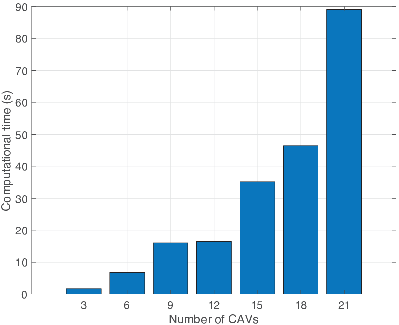
Fig. 3 illustrates the calculated motion trajectories of all CAVs in the second test scenario. As seen, CAVs freely move and use opposite lanes if it is collision-free while avoiding road boundaries. Please check out a provided video on https://youtu.be/L_aFGkKT38U for more details.

The computational time of test scenario two for each number of crossing CAVs is presented in Fig. 4. The presented numbers are the average of 10 times of running the scenario. The standard deviation of the results is less than $0.5\%$ and is not shown. Fig. 4 shows that the computational complexity of the proposed algorithm is of the order of $O(e^{0.13N})$ in terms of number of crossing CAVs $N$. The future work of this study is to reduce the computational time by decentralising the proposed strategy.

References

- Andersson et al. [2019] Andersson, J.A.E., Gillis, J., Horn, G., Rawlings, J.B., Diehl, M., 2019. CasADi – A software framework for nonlinear optimization and optimal control. Mathematical Programming Computation 11, 1–36. doi:10.1007/s12532-018-0139-4.
- Boyd and Vandenberghe [2004] Boyd, S., Vandenberghe, L., 2004. Convex Optimization. Cambridge University Press. doi:10.1017/CBO9780511804441.
- Colombo and Del Vecchio [2012] Colombo, A., Del Vecchio, D., 2012. Efficient algorithms for collision avoidance at intersections, in: Proceedings of the 15th ACM international conference on Hybrid Systems: Computation and Control, pp. 145–154.
- Firoozi et al. [2020] Firoozi, R., Ferranti, L., Zhang, X., Nejadnik, S., Borrelli, F., 2020. A distributed multi-robot coordination algorithm for navigation in tight environments. arXiv preprint arXiv:2006.11492 .
- Li et al. [2020] Li, B., Zhang, Y., Jia, N., Peng, X., 2020. Autonomous intersection management over continuous space: A microscopic and precise solution via computational optimal control. IFAC-PapersOnLine 53, 17071–17076.
- Li et al. [2018] Li, B., Zhang, Y., Zhang, Y., Jia, N., Ge, Y., 2018. Near-optimal online motion planning of connected and automated vehicles at a signal-free and lane-free intersection, in: 2018 IEEE Intelligent Vehicles Symposium (IV), IEEE. pp. 1432–1437.
- Malikopoulos et al. [2021] Malikopoulos, A.A., Beaver, L., Chremos, I.V., 2021. Optimal time trajectory and coordination for connected and automated vehicles. Automatica 125, 109469.
- Malikopoulos et al. [2018] Malikopoulos, A.A., Cassandras, C.G., Zhang, Y.J., 2018. A decentralized energy-optimal control framework for connected automated vehicles at signal-free intersections. Automatica 93, 244–256.
- Milliken and Milliken [1995] Milliken, W., Milliken, D., 1995. Race Car Vehicle Dynamics. Premiere Series, SAE International. URL: https://books.google.co.uk/books?id=opgHfQzlnLEC.
- Mirheli et al. [2019] Mirheli, A., Tajalli, M., Hajibabai, L., Hajbabaie, A., 2019. A consensus-based distributed trajectory control in a signal-free intersection. Transportation research part C: emerging technologies 100, 161–176.
- Pan et al. [2020] Pan, X., Chen, B., Evangelou, S.A., Timotheou, S., 2020. Optimal motion control for connected and automated electric vehicles at signal-free intersections, in: 2020 59th IEEE Conference on Decision and Control (CDC), IEEE. pp. 2831–2836.
- Rios-Torres and Malikopoulos [2016] Rios-Torres, J., Malikopoulos, A.A., 2016. A survey on the coordination of connected and automated vehicles at intersections and merging at highway on-ramps. IEEE Transactions on Intelligent Transportation Systems 18, 1066–1077.
- Rösmann et al. [2020] Rösmann, C., Makarow, A., Bertram, T., 2020. Time-optimal control with direct collocation and variable discretization. arXiv preprint arXiv:2005.12136 .
- Wächter and Biegler [2006] Wächter, A., Biegler, L.T., 2006. On the implementation of an interior-point filter line-search algorithm for large-scale nonlinear programming. Mathematical programming 106, 25–57.
- Zhang et al. [2021a] Zhang, H., Zhang, R., Chen, C., Duan, D., Cheng, X., Yang, L., 2021a. A priority-based autonomous intersection management (aim) scheme for connected automated vehicles (cavs). Vehicles 3, 533–544.
- Zhang et al. [2021b] Zhang, X., Liniger, A., Borrelli, F., 2021b. Optimization-based collision avoidance. IEEE Transactions on Control Systems Technology 29, 972–983.
- Zhang et al. [2017] Zhang, Y., Malikopoulos, A.A., Cassandras, C.G., 2017. Decentralized optimal control for connected automated vehicles at intersections including left and right turns, in: 2017 IEEE 56th Annual Conference on Decision and Control (CDC), IEEE. pp. 4428–4433.