UTF8mc
A Greedy and Optimistic Approach to Clustering
with a Specified Uncertainty of Covariates
Abstract
In this study, we examine a clustering problem in which the covariates of each individual element in a dataset are associated with an uncertainty specific to that element. More specifically, we consider a clustering approach in which a pre-processing applying a non-linear transformation to the covariates is used to capture the hidden data structure. To this end, we approximate the sets representing the propagated uncertainty for the pre-processed features empirically. To exploit the empirical uncertainty sets, we propose a greedy and optimistic clustering (GOC) algorithm that finds better feature candidates over such sets, yielding more condensed clusters. As an important application, we apply the GOC algorithm to synthetic datasets of the orbital properties of stars generated through our numerical simulation mimicking the formation process of the Milky Way. The GOC algorithm demonstrates an improved performance in finding sibling stars originating from the same dwarf galaxy. These realistic datasets have also been made publicly available.
Keywords: Clustering, uncertainty set, optimism, greedy optimization
1 Introduction
The discovery of distinct groups of unlabeled individuals using their covariates, a process called clustering, has been a fundamental statistical problem in the fields of psychology (Borgen and Barnett, 1987; Henry et al., 2005), astronomy (Roederer et al., 2018; Helmi, 2020; Yuan et al., 2020), and biology (Ben-Dor et al., 1999; Nugent and Meila, 2010), among other areas. Owing to its versatility and numerous applications, many types of clustering algorithms have been developed, including -means (MacQueen et al., 1967), mean-shift (Fukunaga and Hostetler, 1975; Cheng, 1995), spectral clustering (Chung, 1997; Von Luxburg, 2007), convex clustering (Pelckmans et al., 2005), and likelihood-based approaches using stochastic block models (Holland et al., 1983) and Gaussian mixture models (McLachlan and Peel, 2000). For comprehensive surveys of various clustering algorithms, see Jain and Dubes, 1988, Everitt, 1993, and Xu and Wunsch, 2005.
Although the aforementioned clustering methods assume that an instance is observed for each individual covariate, in practice, a covariate may have uncertainty caused by limited data observability and noisy measurements. A set representing such uncertainty is called an uncertainty set (Ben-Tal and Nemirovski, 2002; Bertsimas et al., 2011). Robust optimization (RO) (Ben-Tal and Nemirovski, 2002; Bertsimas et al., 2011) is an approach used to exploit an uncertainty set. RO minimizes the worst-case loss functions (over the uncertainty sets for the covariates of all individuals), with application to statistical problems including classification (Xu et al., 2009; Takeda et al., 2013) and clustering (Vo et al., 2016). In contrast to the pessimistic approach of RO, several studies have reported that an optimistic attitude, that is, optimizing the best case (instead of the worst case), demonstrates an improved performance for various problems, including classification (Bi and Zhang, 2004), the multi-armed bandit problem (Bubeck and Cesa-Bianchi, 2012), and Bayesian optimization (Srinivas et al., 2010; Nguyen et al., 2019b; Nguyen et al., 2019a).
For computational tractability, both the pessimistic and optimistic approaches described above employ a convex uncertainty set for each individual covariate, typically a small ball equipped with the -norm () centered at the instance of an observed covariate (Ben-Tal and Nemirovski, 2002; Bertsimas et al., 2011; Vo et al., 2016). Although existing studies have mainly assumed that an uncertainty set is simply a fixed-sized ball around a covariate instance, in practical situations, such uncertainty sets can be specified by background knowledge accumulated over time. We assume here that the uncertainty sets are specified by the users, allowing several entries in some instances to have greater uncertainty than others.
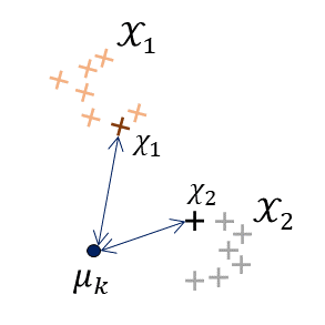
In this study, we consider a clustering problem with covariates whose uncertainty sets for each individual are user-specified. More practically, we consider a situation in which the covariate is further pre-processed by applying a nonlinear function (prior to the clustering analysis) used to capture the latent data structure through the pre-processed feature . This pre-processing step is also expected to remove redundant information harmful to the clustering process. Because the explicit form of an uncertainty set for a pre-processed feature is difficult to obtain, we first generate empirical uncertainty sets that approximate the underlying feature uncertainty sets . To fully exploit them, we propose a simple greedy and optimistic clustering (GOC) algorithm, which greedily seeks feature candidates over the sets that yield more condensed clusters. The proposed GOC algorithm simply iterates the following steps: GOC algorithm (i) computes temporal cluster assignments of the current feature candidates using an arbitrary clustering oracle (e.g., -means or other clustering method listed above), and (ii) updates the feature candidates (and their temporal cluster assignments simultaneously) to reduce each cluster radius.


As an important application of the GOC algorithm, we consider a clustering of stars in the Milky Way to find groups of stars (sibling stars) with similar orbital properties (so-called orbital actions). We generate synthetic datasets of such stars by simulating the formation of the Milky Way. See Example 1 in Section 2 for further details. We apply the GOC algorithm to these realistic datasets to find sibling stars, as illustrated in Figure 1. In comparison to conventional -means applied to the mean vectors of each uncertainty set, the GOC algorithm using -means yields a more condensed clusters of stars. The GOC algorithm also improves the clustering scores. These datasets have also been made publicly available in our repository (https://github.com/oknakfm/GOC).
Although in this study the GOC algorithm is evaluated by leveraging realistic datasets whose true cluster assignments are known, the GOC algorithm has been applied to a real-world orbital action dataset in another study of ours (Hattori et al., 2022), the results of which will be submitted to an astronomy journal.
1.1 Related Works
A similar approach can be found in Ngai et al., 2006, which assumes that the uncertainty set consists of finite points and considers the minimum box ; (a bound of) the Hausdorff distance between the boundary and cluster center is used for -means instead of the Euclidean distance therein. However, Ngai et al., 2006 does not perfectly fit our setting as it implicitly assumes the convexity of the set (also see Section 4.5 for discussion). Another similar approach is possible-world (PW) model, which considers all the possible combinations of feature candidates (called “worlds”) , applies a clustering algorithm for each world (in parallel), and aggregates all the clustering results. See, e.g., Volk et al., 2009, Züfle et al., 2014 and Liu et al., 2021. In contrast to our approach finding only the optimistic candidates, PW models overall require much more computational cost as the number of (even a subset of) possible worlds is numerous.
Another direction for clustering uncertain data employs the probability density function of the feature (). While the simple -means (MacQueen et al., 1967) minimizes the squared Euclidean distance between the feature instance and the cluster centers, UK-means (Chau et al., 2006) considers the expectation of the distance between feature and the cluster centers (with respect to ). As pointed out in Lee et al., 2007 and Cormode and McGregor, 2008, UK-means is equivalent to -means applied to the expectation of features (). Cormode and McGregor, 2008 also provides approximation algorithms for the variants of UK-means (e.g., UK-median). Kriegel and Pfeifle, 2005 and Jiang et al., 2013 define distances between the densities and apply the simlarity-based clustering methods to the proposed distances (also see Section 4.4 for the related approach).
We last note that, clustering uncertain data is distinct from fuzzy clustering (see, e.g., Bezdek, 1981), which outputs multiple assignments of clusters with deterministic input.


2 Problem Setting
Let ; in addition, let denote a set , where also denotes the set of individuals to be clustered. Assume that individual is associated with covariate following a known distribution . Typically, we assume a normal distribution with the observed covariate instance of individual and the positive-definite variance-covariance matrix . Thus, it is reasonable to employ a covariate uncertainty set such that
| (1) |
with a user-specified small threshold parameter . For the uncertainty set, we employ an upper-level set of the probability density function , i.e.,
| (2) |
for some , satisfying the inequality (1). For instance, by assuming that is a Laplace distribution , the set (2) reduces to the box-type uncertainty set used in Vo et al., 2016, and by assuming that is a standard normal distribution, (2) reduces to the Euclidean ball used in Ben-Tal and Nemirovski, 2002. In general, an ellipsoid equipped with a positive definite matrix can be obtained by assuming a normal distribution . Herein, we assume that set is specified in advance for each individual .
To capture the latent data structure, we further consider a pre-processing, that is, the application of a nonlinear transformation into . This pre-processing step is also expected to remove redundant information that is harmful for a clustering analysis. An uncertainty set for this pre-processed feature can be expressed as
| (3) |
which satisfies the following probability inequality:
Interestingly, even if the covariate uncertainty set is convex, the feature uncertainty set (3) does not necessarily inherit the convexity.
Given (1) covariate uncertainty sets for individuals to be clustered, and (2) the nonlinear transformation for pre-processing, our goal is to cluster the individuals by exploiting the feature uncertainty sets . It is possible for the feature uncertainty sets to be non-identical and non-convex, and thus their theoretically explicit forms are difficult to obtain. In this paper, we provide two examples.
Example 1.
In galactic astronomy, it is important to identify groups of stars (sibling stars) with similar orbits in the Milky Way (Roederer et al., 2018; Helmi, 2020). Sibling stars were born in the same dwarf galaxies that were later disrupted and absorbed by the Milky Way; and therefore sibling stars provide an important insight into the history of the Milky Way. Because an orbital period is typically years, humans cannot monitor the entire orbit of a star. Instead, to find sibling stars, we estimate the orbital properties from the instantaneous position (which is an instance of the covariate ) and velocity (which is an instance of ) of each star at the current epoch, by assuming the Galactic gravitational potential. See Figure 3(3) for the six elements in . Usually, we apply a nonlinear function to to derive a three-dimensional quantity called an orbital action , that encapsulates the stellar orbital properties (Binney and Tremaine, 2008). Whereas the position and velocity change as a function of time, the orbital action feature is a conserved quantity (see Figure 8 in Appendix A.2 for an illustration of the conserved orbital actions). Because sibling stars have similar orbital actions, we apply clustering to the pre-processed feature instead of the direct observation . Note that the function omits the remaining information on the instantaneous orbital phase, which does not help in finding sibling stars.


Interestingly, in Example 1, the covariate for the instantaneous position of star may have a larger uncertainty depending on the stellar properties (e.g., fainter stars have a larger uncertainty) or the cadence of the observations (e.g., stars observed less frequently have a larger uncertainty). See Figure 3(3). Therefore, the scatter of the uncertainty set depends on the individual star . We provide synthetic datasets demonstrating Example 1. For further details, see Section 4.1 and Appendix A.
Example 2.
For the general clustering problem of individuals equipped with observed covariate instances (), we can assume that is an instance of the covariate following the distribution , which is typically a normal distribution equipped with a positive-definite variance-covariance matrix . The uncertainty set, , can be specified by (2). To cluster individuals , a nonlinear dimensionality reduction, including a kernel principal component analysis (Schölkopf et al., 1998), can be applied beforehand to the observed covariate instances . Using the nonlinear transformation for a dimensionality reduction (), we obtain the pre-processed feature instance , and the feature uncertainty set can be specified by .
3 Greedy and Optimistic Clustering Algorithm
In Section 3.1, we first define an empirical set that approximates feature uncertainty set through a synthetic data generation over the specified covariate uncertainty set . Using this empirical set, in Section 3.2, we propose the GOC algorithm for clustering with optimism, which exploits a user-specified (arbitrary) clustering oracle . The proposed algorithm equipped with a simple -means clustering is further discussed in Section 3.3.
3.1 Empirical Feature Uncertainty Set
Because of the nonlinear function used in the pre-processing, the theoretically explicit form of the uncertainty set for the pre-processed feature is difficult to obtain. Therefore, we approximate set through synthetic data generation using the user-specified set and nonlinear function .
To approximate set , we employ instances of the -dimensional random variable following a uniform distribution over set , i.e.,
| (4) |
and define an empirical feature uncertainty set as follows:
| (5) |
are hyperparameters, typically, . By assuming the following non-degenerate condition on function with the Lebesgue measure (over the -dimensional Euclidean space ), i.e.,
| (6) |
proposition 1 proves that the set approximates the uncertainty set .
Proposition 1.
Assume that satisfies the non-degenerate condition (6). For any , it holds that in probability, for .
Proof.
Let be a ball centered at with radius ; in addition, let denote the complement of set . This assertion is proved by for for any because follows from the condition (6). ∎
Taking an arbitrary feature instance , the set with a sufficiently large has an entry sufficiently close to , for which we can expect that
| (7) |
for a wide class of functions . This proposition can be applied to (8) in GOC (under some mild assumptions).
3.2 Greedy and Optimistic Clustering Algorithm
In this section, we propose a greedy and optimistic clustering (GOC) algorithm, that greedily seeks the feature candidates over a set
yielding more condensed clusters. Given the initial feature candidates , initial number of clusters , initial cluster assignments , and an user-specified arbitrary clustering oracle (e.g., -means), which outputs the cluster assignments of individuals by taking an instance (as well, we can input the number of clusters , initial cluster centers, and some additional parameters, if necessary), GOC iterates the following steps: at iteration ,
- (I)
The designated number of clusters is updated. Typically, we may employ a constant or the number of clusters found in the previous step .
- (II)
Temporal cluster assignments are obtained using the clustering oracle:
- (III)
Feature candidates and cluster assignments are updated to and , respectively, by applying
(8) , where
(9) denotes the cluster center, denotes a user-specified penalty term (e.g., for some ), and is a hyperparameter. Note that the penalty term may depend on the individual .
Steps (I)–(III) are repeated until convergence is reached. See Figure 4 for an illustration, and Section 3.3 for an interpretation of the GOC algorithm using -means clustering.


Computational complexity.
Step (II) requires the computational complexity to be exactly the same as the clustering oracle (typically, ), and step (III) can be solved through a linear search, which requires complexity (typically smaller than ). Therefore, the overall complexity is approximately with iterations, where is a sufficient number in our numerical experiments, as demonstrated in Experiment 3 described in Section 4.
3.3 Interpretation of GOC Algorithm with -means Clustering
In this section, we interpret the results of the proposed GOC algorithm using -means clustering (MacQueen et al., 1967) with a constant number of clusters . Let
be a set of cluster-assignment indicators , where denotes that individual is assigned to cluster (and otherwise). Using a loss function
conventional -means clustering applied to a fixed instance computes the cluster assignments by solving the following problem:
Further, the GOC algorithm equipped with -means clustering is expected to solve the following minimization problem in a greedily manner:
for . By contrast, we may consider a pessimistic variant of the GOC algorithm, i.e., the greedy and pessimistic clustering (GPC), when solving the following problem:
the formulation of which achieves a robust optimization (Ben-Tal and Nemirovski, 2002; Bertsimas et al., 2011), minimizing the worst-case of the loss function. Furthermore, assuming that (i.e., no penalty for the candidates ) and is a box-shaped convex uncertainty set with a user-specified small threshold parameter , GPC greedily solves the equivalent problem described in Vo et al., 2016, which is the only existing study applying robust optimization to clustering.
However, note that the set considered in this study is not the small box-shaped convex set considered in Vo et al., 2016 (where Vo et al., 2016 aims to attain robustness against a covariate perturbation but not the larger uncertainty considered herein), and the GPC applied to our synthetic dataset achieved extremely low scores. In particular, because the feature candidates are updated to increase the scattering of each cluster from a pessimistic perspective, regardless of the initial number of clusters , GPC applied to our dataset finally outputs only one large cluster (i.e., after a sufficiently large number of iterations ). We therefore did not apply GPC in our numerical experiments, as discussed in Section 4.
4 Numerical Experiments
In Section 4.1, we describe the synthetic orbital action datasets of the stars used in our numerical experiments.
The experimental settings and results are presented in Sections 4.2 and 4.3, respectively.
Further disccusions are also provided: we consider another approach for exploiting the uncertainty sets in Section 4.4 and
convex feature ambiguity sets in Section 4.5.
We provide the datasets and R source codes used to produce the experimental results at https://github.com/oknakfm/GOC.
4.1 Realistic Datasets: Orbital Properties of the Stars in the Milky Way
We employed synthetic orbital action datasets of stars generated through a numerical simulation mimicking the formation process of the Milky Way. Each of these datasets consists of pre-computed empirical uncertainty sets with stars, where each star is assigned to one of true clusters and is associated with the empirical uncertainty set of size . The member stars of each true cluster are born in the same dwarf galaxy, which we refer to as sibling stars. Sibling stars have similar orbital actions (i.e., similar orbital properties), and our task is to find sibling stars by leveraging uncertainty sets. Figure 5 shows the first three datasets used.


In addition to a summary of this dataset, Appendix A provides more detailed descriptions of the physical simulation.
Summary of a dataset is described herein: we generate different datasets by following the same procedure. We generate the uncertainty sets of stars, which form clusters with similar orbits. Following the numerical simulation shown in Appendix A, we obtain the instance , consisting of the true current position and velocity of the th star () within the observable space. Note that the observable space differs from the usual Cartesian coordinate system. For example, in astronomy, the three-dimensional stellar position is expressed by the so-called stellar parallax (which is the reciprocal of the stellar distance from Earth ) and the two-dimensional position in the sky. See Figure 3(3) for an illustration. The observational uncertainty in is denoted as and is computed from the empirical relationship known in the field of galactic astronomy (see Gaia Collaboration et al., 2021). Note that, owing to observational difficulty, one of the three components in (stellar parallax) is associated with a large uncertainty, whereas the other two components in (two-dimensional position in the sky) and all three components in are associated with negligible uncertainty.
To mimic an actual observation in which we do not know the true value of each observable, we incorporate randomness into the quantity , i.e., each entry in is drawn independently from . Subsequently, we define the uncertainty set as follows:
and draw i.i.d. instances from a uniform distribution for .
Finally, we compute the empirical uncertainty set using Eq. (5); that is,
.
In particular, to transform the current positions and velocities of the stars into orbital actions, we employ a publicly available AGAMA package (Vasiliev, 2018; Vasiliev, 2019) for the nonlinear transformation ,
which effectively removes unnecessary information for finding clusters of sibling stars.
In the simplest implementation of the GOC algorithm, we can treat all elements of the uncertainty set for star equally. However, we can introduce a penalty term to prioritize (penalize) the elements of an uncertainty set that are closer to (farther from) the center of the uncertainty set, . For this purpose, we define the penalty of the th candidate of star as . Note that, because its uncertainty is the dominant source of uncertainty in , we only consider the first component of , which corresponds to the stellar parallax.
4.2 Experimental Settings
Standardization.
Before conducting the experiments, we first standardize the empirical uncertainty sets (using both centering and scaling, such that ) and the penalties (using scaling only, such that ) for each dataset.
Clustering oracles.
We employ -means (using the standard stats package in R statistical software) and
-medoids (using the ClusterR package), which can take the cluster centers as their input, and for each iteration, we input the cluster center .
We also employ two different implementations of a Gaussian mixture model(GMM), i.e.,
the GMM function in the ClusterR package, and the Mclust function in the mclust package, the latter of which (Mclust) can specify models for the variance-covariance matrix of the Gaussian distribution (representing the cluster ).
We employ the simplest EII model ( for a certain ; more general VII and VVV models are also mentioned in the note of Experiment 4), and Mclust automatically detects the number of clusters using BIC (from ). See Scrucca et al., 2016 for further details.
Baselines.
For the baselines, we apply clustering oracles (-means, -medoids, and GMM) to the vectors
| (10) |
which represent the sample mean of each feature uncertainty set. Referring to Lee et al., 2007, the -means applied to (10) also can be regarded as UK-means (Chau et al., 2006) by assuming that the feature follows a uniform distribution over the set (for ).
Evaluation metrics.
We define the following scores, using the estimated clusters as well as the true clusters , , , and .
- 1.
Normalized mutual information is defined by , using the mutual information and entropy :
- 2.
The -measure is defined as
Both the NMI and -measure take values within , and attain a value of if and only if the estimated clusters perfectly match the true clusters (up to the permutation of the cluster labels).
Additional settings.
The clustering step used by the GOC algorithm employs the number of clusters appearing in the previous step, i.e., , and thus the number of clusters for the algorithm can be smaller than the (user-specified) initial number of clusters . We consider the GOC algorithm to reach convergence if the selected feature candidates are converged. More specifically, in Experiments , , and , we consider the perfect convergence of the feature candidates (selected from the discrete set ); by allowing a tolerance on the convergence, we can terminate GOC with fewer iterations as observed in Experiment .
4.3 Experimental Results
We apply the GOC algorithm along with the clustering oracle to synthetic datasets consisting of empirical uncertainty sets. For the baselines, we also apply the oracle to the representative vectors defined in (10). Whereas Experiments 1–3 computed only the GOC algorithm when applying -means (as well as the corresponding baseline, i.e., -means applied to the representative vectors), -medoids and GMM were applied in Experiment 4.
Experiment 1: Fixed with increasing .
Table 1(c) shows the NMI and -measure with a fixed initial number of clusters and increasing (the coefficient of the penalty term).
| NMI | GOC | ||||
|---|---|---|---|---|---|
| Baseline | |||||
| -measure | GOC | ||||
| Baseline | , | ||||
| clusters | GOC | ||||
| iterations | GOC | ||||
| NMI | GOC | ||||
|---|---|---|---|---|---|
| Baseline | , | ||||
| -measure | GOC | ||||
| Baseline | |||||
| clusters | GOC | ||||
| iterations | GOC | ||||
| NMI | GOC | ||||
|---|---|---|---|---|---|
| Baseline | |||||
| -measure | GOC | ||||
| Baseline | |||||
| clusters | GOC | ||||
| iterations | GOC | ||||
Results.
First, for the experiments with a small , the proposed GOC algorithm outperforms the baselines. Employing feature uncertainty sets also improves the NMI and -measure. A large coefficient of the penalty term degrades both the NMI and the -measure; in addition, clustering with stars having a smaller penalty does not necessarily improve the clustering scores. Although the number of clusters used by the GOC algorithm can be small, the number is not significantly different from the initial number of clusters .
Experiment 2: Fixed with increasing .
Table 2 shows the NMI and -measure with a fixed and increased number of initial clusters .
| NMI | GOC | |||||
|---|---|---|---|---|---|---|
| Baseline | ||||||
| -measure | GOC | |||||
| Baseline | ||||||
| clusters | GOC | |||||
| iterations | GOC |
Results.
Because the true number of clusters is , both the GOC algorithm and the baselines demonstrate a better performance with than with . Overall, with , fewer iterations are required (for GOC convergence) for a larger , and a larger tends to result in higher scores.
Experiment 3: Convergence.
Although the convergence of the GOC algorithm is determined by the perfect convergence of the feature candidates in Experiments and (because the candidates are selected over the discrete set ), we monitored the convergence of the GOC algorithm in a weaker sense. In particular, we monitored the convergences of (1) the cluster assignments and (2) the feature candidates. To evaluate the convergence, for each dataset, we computed two scores and , where denote the final cluster assignments and feature candidates of the GOC algorithm, respectively. We also computed the convergence of the NMI scores to the underlying true clusters by evaluating . Figure 6 shows these scores (for each iteration ) for datasets for with a fixed .
Results.
Although Experiments 1 and 2 show that almost iterations are required for the GOC algorithm to completely converge, both the cluster assignments and feature candidates almost converge within iterations (specifically, the feature candidates almost converge within iterations). NMI also nearly converges within iterations, and only – iterations are required for the GOC algorithm to obtain a sufficient performance during these experiments.
Experiment 4: Comparison to other clustering oracles.
Table 3(c) computes the GOC algorithm and the corresponding baselines for other clustering oracles (-medoids and the GMM using the ClusterR and Mclust packages). Note that the GMM (Mclust+BIC) selects the number of clusters using BIC (from ) in each clustering step.
| -means | -medoids | GMM (ClusterR) |
GMM (Mclust+BIC) | ||
|---|---|---|---|---|---|
| NMI | GOC | ||||
| Baseline | |||||
| -measure | GOC | ||||
| Baseline | |||||
| clusters | GOC | ||||
| iterations | GOC |
| -means | -medoids | GMM (ClusterR) |
GMM (Mclust+BIC) | ||
|---|---|---|---|---|---|
| NMI | GOC | ||||
| Baseline | |||||
| -measure | GOC | ||||
| Baseline | |||||
| clusters | GOC | ||||
| iterations | GOC |
| -means | -medoids | GMM (ClusterR) |
GMM (Mclust+BIC) | ||
|---|---|---|---|---|---|
| NMI | GOC | ||||
| Baseline | |||||
| -measure | GOC | ||||
| Baseline | |||||
| clusters | GOC | ||||
| iterations | GOC |
Results.
For all clustering oracles, the proposed GOC algorithm improves the clustering scores by simply applying the oracle to the representative vectors (baseline).
In addition, -means and -medoids demonstrate almost the same performance for , whereas -means requires slightly fewer iterations to converge.
We think that the vector used to update the feature vectors is more compatible with -means by minimizing the simple -norm between the features and the cluster centers.
GMM (ClusterR) demonstrates a similar performance as -means and -medoids, all of which detect almost the same number of clusters.
GMM (MClust+BIC) detects fewer clusters than -means, -medoids, and GMM (ClusterR).
GMM (MClust+BIC) also achieves lower scores, whereas GMM (Mclust+BIC) tends to detect the same cluster assignments and feature representative during the first iteration, regardless of (because it selects the number of clusters using BIC).
Note that the number of underlying true clusters is , i.e., BIC applied to GMM (Mclust) underestimates the number of clusters.
See Appendix B for the convergence experiments conducted on -medoids, GMM (ClusterR), and GMM (Mclust+BIC).
Notes on Experiment 4.
While we employed the EII model () for , we also conducted experiments on the Mclust function with more general models, i.e., VII ( for ) and VVV (where can be arbitrary): VVV generalizes VII, and VII generalizes EII.
Under the setting , NMI scores for the GOC algorithm using GMM (Mclust(VII)+BIC) and GMM (Mclust(VVV)+BIC) are and , respectively, whereas the detected numbers of clusters are and . Therefore, the scores are in the order of EIIVIIVVV, which is opposite the model degrees of freedom, which are in the order of EIIVIIVVV.
4.4 Discussion 1: Similarity-based Clustering
As another way to exploit the feature uncertainty, Kriegel and Pfeifle, 2005 and Jiang et al., 2013 define discrepancies between the probability densities of features and apply similarity-based clustering algorithms. However, we cannot employ this approach in our setting, as the explicit forms of the densities are hardly obtained due to the non-linear pre-processing. Therefore, as an alternative implementation, we measure the discrepancy between the feature uncertainty sets, and apply affinity propagation (Frey and Dueck, 2007, AP;) which takes the similarity matrix as its input and outputs the estimated clusters.
To compute the similarity matrix, for , we employ the negative sign of the following three types of discrepancies between :
The last one is known as the Hausdorff distance.
The AP was implemented using the apcluster package in R.
Therein, exemplar preferences are set to the sample quantile of the input dissimilarities with a threshold ; in addition, we employ .
Table 4 shows the NMI and -measure for the baseline (-means applied to the representative vectors (10)), and the AP equipped with negative signs of .
For the baseline and GOC algorithm, we set and , respectively.
| NMI | -measure | clusters | ||
| GOC | ||||
| Baseline | ||||
| AP () | ||||
| AP () | ||||
| AP () | ||||
Results.
Although the GOC algorithm outperforms all AP clustering scores, the AP with demonstrates a competitive performance (although the AP with a larger of greater than unfortunately tends to become unstable). The AP equipped with and demonstrates good clustering scores. In fact, the discrepancy does not satisfy the triangle inequality (namely, is not the distance between and ), unlike and . Therefore, for several specific situations, as an alternative to the proposed GOC algorithm, we admit the potential significance of distance-based clustering approaches endowed with some specific dissimilarities (that are not restricted to satisfying the definitions of distance ).
Finally, we note that the complexity when computing the distances between pairs of ambiguity sets is large. The complexity is when assuming that , whereas the GOC algorithm roughly requires with iterations (in our numerical experiments, and , whereby ). Computing the similarities of the ambiguity sets is rather burdensome if and increase.
4.5 Discussion 2: Convex Uncertainty Sets
While we employ the empirical uncertainty set which is not restricted to be convex, we may consider an alternative convex set containing : finding possible feature candidates over the set
instead of , is expected to be more efficiently computed by the existing optimization techniques related to convex sets. For computational reasons, Ngai et al., 2006 considers a minimum box containing as the convex set , and Vo et al., 2016 assumes that the uncertainty set is box-shaped (i.e., convex).
Referring to Vo et al., 2016, we may employ difference-of-convex algorithm (Le Thi and Tao, 2005, DCA; see, e.g.,) to solve a specific form of GOC (particularly, GOC equipped with -means) more efficiently. We think that this convex modification of GOC would be a future research worth considering, while we do not employ this convex set in this study by the following reasons: (i) to exploit the convex techniques, we need to heavily restrict the types of clustering oracle (whereby the applicability of GOC would be much degraded, and the implementation would be mathematically difficult for users), and (ii) the convex set may contain large unnecessary regions in some situations (see Figure 7).


5 Conclusion
This study considered a clustering problem using user-specified uncertainty for the covariates. In particular, we considered a pre-processing that applies a non-linear transformation to the covariates to obtain features that are expected to capture the latent data structure. In addition, we proposed the GOC algorithm, which greedily finds better feature candidates over the uncertainty sets (of the pre-processed features). We applied the GOC algorithm to a synthetic orbital action dataset of sibling stars generated through our numerical simulation, for which the proposed algorithm improved the clustering scores. We also provided realistic datasets and source codes to reproduce the experimental results in https://github.com/oknakfm/GOC.
Finally, we describe below the limitations and possible extensions of this study.
Limitations.
We must specify and when applying the GOC algorithm.
Specifying the number of clusters is a common and historical problem in computational statistics (for instance, see Thorndike, 1953 for the elbow method, and inexhaustible discussions have been developed for several decades).
Although we may simply apply the existing approaches to each clustering step, the number of clusters detected depends on the feature candidate at a particular step under our problem setting, and it remains unclear whether the conventional approaches are still effective.
The BIC used in the Mclust implementation of the GMM underestimates the number of clusters, as shown through Experiment 4 described in Section 4.3. Because clustering is an unsupervised problem, regarding the selection of hyperparameter , we cannot employ standard statistical approaches such as a cross-validation.
Although our experiment results show the adequacy of using a small (even a of 0 is effective with our datasets), we have yet to sufficiently confirm this.
Possible extensions of this research.
A possible extension of this study would be to accelerate the speed of the GOC algorithm. Because most of the clustering algorithms considered in this study (i.e., -means, -medoids, and GMM) use iterative algorithms, we can terminate the iterations in each clustering oracle before convergence is reached. Namely, we can reduce the number of unnecessary iterations (within each clustering step) and focus more on the convergence in the sense of the overall GOC. Another possible extension of this research is to incorporate hierarchical clustering into the GOC algorithm. Because the iterations of the algorithm easily break down the hierarchical structure found during the clustering step, some modifications of the algorithm are needed to obtain the hierarchical structure of the GOC output.
Acknowledgement
AO was supported by JSPS KAKENHI (Grant No. JP21K17718) and JST CREST (Grant No. JPMJCR21N3). KH was also supported by JSPS KAKENHI (Grant Nos. JP21K13965 and JP21H00053). We would like to thank Keisuke Yano for helpful discussion
Appendix A Detailed Descriptions of Synthetic Dataset
A.1 General Description of the Simulation
In galactic astronomy, it is believed that the Milky Way was formed through the merging of smaller systems, such as dwarf galaxies. In the numerical experiments described in Section 4.1, we generated mock data by simulating the formation process of the Milky Way. To simplify this case, we assume that dwarf galaxies merge with the Milky Way and are instantaneously disrupted at time . Each dwarf galaxy contains 30,000 sibling stars. When a dwarf galaxy is disrupted, sibling stars begin moving independently. After , and until the current epoch ( years), the motions of these sibling stars are treated as test particles (i.e., particles with zero mass) moving within the gravitational potential of the Milky Way. For each dwarf galaxy, the positions and velocities of the sibling stars at (i.e., the initial conditions) slightly differ from each other. The small difference in the initial conditions evolves over cosmic time, and the positions and velocities of the sibling stars are completely different from each other in the current epoch, although they originate from the same dwarf galaxy.
A.2 Visualization of the Simulation
To provide an intuitive understanding of the simulation, Figure 8 shows a subset of sibling stars in two dwarf galaxies A and B that merge with the Milky Way at . At , the sibling stars in each dwarf galaxy have identical positions and slightly different velocities, making these two groups clearly distinguishable in terms of their positions and velocities. At years, the positions and velocities of the sibling stars exhibit a wider distribution, and the two groups of stars are marginally distinguishable in terms of their positions and velocities. At the current epoch, years, the positions and velocities of the sibling stars show a mixed distribution. At this point, it is difficult to separate two groups of stars from each other in terms of their positions and velocities.
From these three snapshots, it is evident that finding sibling stars within a six-dimensional position and velocity space becomes more difficult as the system evolves over time. Importantly, this difficulty is unrelated to the accuracy of the data. Even if we have a perfect measurement of the positions and velocities of the stars, finding sibling stars is a difficult task if we use the raw data of position and velocity.
However, the case appears to be simpler if we look at the system in a three-dimensional phase space spanned by the orbital action. (As a reminder of the readers, the orbital action is a three-dimensional conserved quantity, which is a function of position and velocity; and it describes the stellar orbital properties.) Because the orbital action is conserved for each star, the distribution of sibling stars in the orbital action space is also conserved over time, as shown in the rightmost panels in Figure 8. Therefore, using the action distribution instead of the position and velocity distributions is an indispensable strategy for identifying sibling stars. As shown in Example 1, in the presence of observational uncertainties in the stellar positions and velocities, it is difficult to find sibling stars in the action space, which motivated us to introduce the GOC algorithm as a new type of clustering approach.

A.3 Detailed Implementations of the Simulation
To generate mock data, we first randomly generated centroids with positions and velocities () using a realistic distribution function model of the Milky Way, similar to that described in Hattori et al., 2021. The th centroid corresponds to the position and velocity of the th dwarf galaxy at . For the th dwarf galaxy, we generated positions and velocities, and (), such that and with . Here, denotes the identity matrix. These positions and velocities correspond to the initial conditions of the sibling stars at . From these initial conditions, we integrated the orbits of stars for years (which is approximately the age of the universe) under a widely used gravitational potential model of the Milky Way described in McMillan, 2017 and derived the current-day positions and velocities. At this point, stars originating from the same dwarf galaxy are no longer located close to each other (see the bottom-left panel in Figure 8). To mimic the observations, for the th group, we randomly select stars that are close to the current position of the Sun. (Note that stars that are too far away from the Sun are too faint to be observed.) The assumed position and velocity of the Sun is the same as those in Doke and Hattori, 2022. We chose , where “” denotes the residual of the division ( divided by ). With this, we have stars in total, such that we have 1 member star for ; we have 2 member stars for ; and so on.
For completeness, in the following, we briefly mention how we converted the simulated data into the uncertainty set used by the GOC algorithm. (See Section 4.1 for a full description.) First, we converted the simulated stellar positions and velocities of stars into observable quantities, as illustrated schematically in Figure 3(3). Note that the stellar positions and velocities in the simulation are true quantities that are unavailable in reality. To mimic the actual observation, we add a random error to the observable quantities, which are then used to construct the uncertainty set.
By following the same procedure, we run 10 independent simulations. Each simulation is used to construct a dataset.
Appendix B Convergence of GOC Using -Medoids and GMM
Regarding the comparison of the convergence of the -means clustering shown through Experiment 3 described in Section 4.3, Figures 11–11 show the convergence of -medoids, GMM (ClusterR), and GMM (Mclust+BIC), respectively, all of which demonstrated the same tendencies.
ClusterR).Mclust+BIC).References
- Ben-Dor et al., (1999) Ben-Dor, A., Shamir, R., and Yakhini, Z. (1999). Clustering gene expression patterns. Journal of Computational Biology, 6(3-4):281–297.
- Ben-Tal and Nemirovski, (2002) Ben-Tal, A. and Nemirovski, A. (2002). Robust optimization–methodology and applications. Mathematical Programming, 92(3):453–480.
- Bertsimas et al., (2011) Bertsimas, D., Brown, D. B., and Caramanis, C. (2011). Theory and applications of robust optimization. SIAM review, 53(3):464–501.
- Bezdek, (1981) Bezdek, J. C. (1981). Pattern Recognition with Fuzzy Objective Function Algorithms. Springer Science & Business Media.
- Bi and Zhang, (2004) Bi, J. and Zhang, T. (2004). Support vector classification with input data uncertainty. In Advances in Neural Information Processing Systems, volume 17. MIT Press.
- Binney and Tremaine, (2008) Binney, J. and Tremaine, S. (2008). Galactic Dynamics. Princeton University Press, second edition.
- Borgen and Barnett, (1987) Borgen, F. H. and Barnett, D. C. (1987). Applying cluster analysis in counseling psychology research. Journal of Counseling Psychology, 34(4):456–468.
- Bubeck and Cesa-Bianchi, (2012) Bubeck, S. and Cesa-Bianchi, N. (2012). Regret analysis of stochastic and nonstochastic multi-armed bandit problems. Foundations and Trends in Machine Learning, 5(1):1–122.
- Chau et al., (2006) Chau, M., Cheng, R., Kao, B., and Ng, J. (2006). Uncertain data mining: An example in clustering location data. In Proceedings of the 10th Pacific-Asia Conference on Advances in Knowledge Discovery and Data Mining, page 199–204, Berlin, Heidelberg. Springer-Verlag.
- Cheng, (1995) Cheng, Y. (1995). Mean shift, mode seeking, and clustering. IEEE Transactions on Pattern Analysis and Machine Intelligence, 17(8):790–799.
- Chung, (1997) Chung, F. R. K. (1997). Spectral Graph Theory. American Mathematical Society.
- Cormode and McGregor, (2008) Cormode, G. and McGregor, A. (2008). Approximation algorithms for clustering uncertain data. In Proceedings of the Twenty-Seventh ACM SIGMOD-SIGACT-SIGART Symposium on Principles of Database Systems, page 191–200, New York, NY, USA. Association for Computing Machinery.
- Doke and Hattori, (2022) Doke, Y. and Hattori, K. (2022). Probability of forming gaps in the GD-1 stream by close encounters of globular clusters. arXiv e-prints, page arXiv:2203.15481.
- Everitt, (1993) Everitt, B. (1993). Cluster Analysis. Edward Arnold, third edition.
- Frey and Dueck, (2007) Frey, B. J. and Dueck, D. (2007). Clustering by passing messages between data points. Science, 315(5814):972–976.
- Fukunaga and Hostetler, (1975) Fukunaga, K. and Hostetler, L. (1975). The estimation of the gradient of a density function, with applications in pattern recognition. IEEE Transactions on Information Theory, 21(1):32–40.
- Gaia Collaboration et al., (2021) Gaia Collaboration, Brown, A. G. A., Vallenari, A., Prusti, T., et al. (2021). Gaia Early Data Release 3. Summary of the contents and survey properties. Astronomy & Astrophysics, 649:A1.
- Hattori et al., (2022) Hattori, K., Okuno, A., and Roederer, I. (2022). Optimisitic clustering - a new clustering method to find structures in noisy data set: An application to clustering analysis of -II halo stars in the milky way. in prep.
- Hattori et al., (2021) Hattori, K., Valluri, M., and Vasiliev, E. (2021). Action-based distribution function modelling for constraining the shape of the Galactic dark matter halo. Monthly Notices of the Royal Astronomical Society, 508(4):5468–5492.
- Helmi, (2020) Helmi, A. (2020). Streams, Substructures, and the Early History of the Milky Way. Annual Review of Astronomy and Astrophysics, 58:205–256.
- Henry et al., (2005) Henry, D. B., Tolan, P. H., and Gorman-Smith, D. (2005). Cluster analysis in family psychology research. Journal of Family Psychology, 19(1):121–132.
- Holland et al., (1983) Holland, P. W., Laskey, K. B., and Leinhardt, S. (1983). Stochastic blockmodels: First steps. Social Networks, 5(2):109–137.
- Jain and Dubes, (1988) Jain, A. K. and Dubes, R. C. (1988). Algorithms for Clustering Data. Prentice-Hall, Inc., USA.
- Jiang et al., (2013) Jiang, B., Pei, J., Tao, Y., and Lin, X. (2013). Clustering uncertain data based on probability distribution similarity. IEEE Transactions on Knowledge and Data Engineering, 25(4):751–763.
- Kriegel and Pfeifle, (2005) Kriegel, H.-P. and Pfeifle, M. (2005). Density-based clustering of uncertain data. In Proceedings of the Eleventh ACM SIGKDD International Conference on Knowledge Discovery in Data Mining, page 672–677, New York, NY, USA. Association for Computing Machinery.
- Le Thi and Tao, (2005) Le Thi, H. A. and Tao, P. (2005). The DC (difference of convex functions) programming and DCA revisited with DC models of real world nonconvex optimization problems. Annals of Operations Research, 133:23–46.
- Lee et al., (2007) Lee, S. D., Kao, B., and Cheng, R. (2007). Reducing UK-means to K-means. In Seventh IEEE International Conference on Data Mining Workshops, pages 483–488.
- Liu et al., (2021) Liu, H., Zhang, X., Zhang, X., Li, Q., and Wu, X.-M. (2021). RPC: Representative possible world based consistent clustering algorithm for uncertain data. Computer Communications, 176:128–137.
- MacQueen et al., (1967) MacQueen, J. et al. (1967). Some methods for classification and analysis of multivariate observations. In Proceedings of the Fifth Berkeley Symposium on Mathematical Statistics and Probability, volume 1, pages 281–297. Oakland, CA, USA.
- McLachlan and Peel, (2000) McLachlan, G. J. and Peel, D. (2000). Finite mixture models. Wiley Series in Probability and Statistics, New York.
- McMillan, (2017) McMillan, P. J. (2017). The mass distribution and gravitational potential of the Milky Way. Monthly Notices of the Royal Astronomical Society, 465(1):76–94.
- Ngai et al., (2006) Ngai, W. K., Kao, B., Chui, C. K., Cheng, R., Chau, M., and Yip, K. Y. (2006). Efficient clustering of uncertain data. In Proceedings of the Sixth International Conference on Data Mining, pages 436–445.
- (33) Nguyen, V. A., Shafieezadeh Abadeh, S., Yue, M.-C., Kuhn, D., and Wiesemann, W. (2019a). Calculating optimistic likelihoods using (geodesically) convex optimization. In Advances in Neural Information Processing Systems, volume 32. Curran Associates, Inc.
- (34) Nguyen, V. A., Shafieezadeh Abadeh, S., Yue, M.-C., Kuhn, D., and Wiesemann, W. (2019b). Optimistic distributionally robust optimization for nonparametric likelihood approximation. In Advances in Neural Information Processing Systems, volume 32. Curran Associates, Inc.
- Nugent and Meila, (2010) Nugent, R. and Meila, M. (2010). An overview of clustering applied to molecular biology. Statistical Methods in Molecular Biology, pages 369–404.
- Pelckmans et al., (2005) Pelckmans, K., De Brabanter, J., Suykens, J. A., and De Moor, B. (2005). Convex clustering shrinkage. In PASCAL Workshop on Statistics and Optimization of Clustering Workshop.
- Roederer et al., (2018) Roederer, I. U., Hattori, K., and Valluri, M. (2018). Kinematics of Highly r-process-enhanced Field Stars: Evidence for an Accretion Origin and Detection of Several Groups from Disrupted Satellites. The Astronomical Journal, 156(4):179.
- Schölkopf et al., (1998) Schölkopf, B., Smola, A., and Müller, K.-R. (1998). Nonlinear component analysis as a kernel eigenvalue problem. Neural Computation, 10(5):1299–1319.
- Scrucca et al., (2016) Scrucca, L., Fop, M., Murphy, T. B., and Raftery, A. E. (2016). mclust 5: clustering, classification and density estimation using Gaussian finite mixture models. The R Journal, 8(1):289–317.
- Srinivas et al., (2010) Srinivas, N., Krause, A., Kakade, S. M., and Seeger, M. W. (2010). Gaussian process optimization in the bandit setting: No regret and experimental design. In Proceedings of the 27th International Conference on Machine Learning.
- Takeda et al., (2013) Takeda, A., Mitsugi, H., and Kanamori, T. (2013). A unified classification model based on robust optimization. Neural Computation, 25(3):759–804.
- Thorndike, (1953) Thorndike, R. L. (1953). Who belongs in the family. Psychometrika, 18(4):267–276.
- Vasiliev, (2018) Vasiliev, E. (2018). AGAMA: Action-based galaxy modeling framework.
- Vasiliev, (2019) Vasiliev, E. (2019). AGAMA: Action-based galaxy modelling architecture. Monthly Notices of the Royal Astronomical Society, 482(2):1525–1544.
- Vo et al., (2016) Vo, X. T., Le Thi, H. A., and Pham Dinh, T. (2016). Robust optimization for clustering. In Intelligent Information and Database Systems, pages 671–680, Berlin, Heidelberg. Springer Berlin Heidelberg.
- Volk et al., (2009) Volk, P. B., Rosenthal, F., Hahmann, M., Habich, D., and Lehner, W. (2009). Clustering uncertain data with possible worlds. In IEEE 25th International Conference on Data Engineering, pages 1625–1632.
- Von Luxburg, (2007) Von Luxburg, U. (2007). A tutorial on spectral clustering. Statistics and Computing, 17(4):395–416.
- Xu et al., (2009) Xu, H., Caramanis, C., and Mannor, S. (2009). Robustness and regularization of support vector machines. Journal of Machine Learning Research, 10(51):1485–1510.
- Xu and Wunsch, (2005) Xu, R. and Wunsch, D. (2005). Survey of clustering algorithms. IEEE Transactions on Neural Networks, 16(3):645–678.
- Yuan et al., (2020) Yuan, Z., Myeong, G. C., Beers, T. C., Evans, N. W., Lee, Y. S., Banerjee, P., Gudin, D., Hattori, K., Li, H., Matsuno, T., Placco, V. M., Smith, M. C., Whitten, D. D., and Zhao, G. (2020). Dynamical Relics of the Ancient Galactic Halo. Astrophysical Journal, 891(1):39 (17pp).
- Züfle et al., (2014) Züfle, A., Emrich, T., Schmid, K. A., Mamoulis, N., Zimek, A., and Renz, M. (2014). Representative clustering of uncertain data. In Proceedings of the 20th ACM SIGKDD International Conference on Knowledge Discovery and Data Mining, pages 243–252, New York, NY, USA. Association for Computing Machinery.