Dynamics of co-orbital exoplanets in a first order resonance chain with tidal dissipation

In order to define a canonical coordinate system related to the semimajor axis $a_{j}$, the eccentricity $e_{j}$, the mean longitude $\lambda_{j}$ and the longitude of the pericentre $\varpi_{j}$ of planet $j$, we first consider Poincaré heliocentric coordinates ($\tilde{\Lambda}_{j},\lambda_{j},\tilde{D}_{j},-\varpi_{j}$) where

In these coordinates, the Hamiltonian derives from the symplectic form

Following Laskar and Robutel, 1995, the planetary Hamiltonian is written

where the Keplerian part, due to star-planet interactions, reads

and the perturbation $H_{P}$, whose size relative to $H_{K}$ is of order $\left(m_{1}+m_{2}+m_{3}\right)/m_{0}$, is expanded in power series of the eccentricities. We assume that the system is close to the resonance $p:p:p+1$. This means that the nominal mean motions verify

while the nominal semimajor axes $a_{j,0}$ are related to $n_{j,0}$ by the “Kepler law” $n_{j,0}^{2}a_{j,0}^{3}=\mu_{0}=\mathcal{G}m_{0}$. The $a_{j}$ are always close to their nominal value²² 2 The nominal semimajor axes are defined with $\mu_{0}$ instead of $\mu_{j}$, which conveniently yields $a_{1,0}=a_{2,0}$. This approximation is valid since the subsequent error is of order $\mathcal{O}\left(m_{j}/m_{0}\right)$, while the width of the resonance is of order $\mathcal{O}\sqrt{m_{j}/m_{0}}$. $a_{j,0}$, and the $\tilde{\Lambda}_{j}$ stay close to the quantities $\Lambda_{j}^{\star}$ defined as

To study the dynamics in the vicinity of the resonance, we expand the Hamiltonian in the neighbourhood of $\left(\Lambda_{1}^{\star},\Lambda_{2}^{\star},\Lambda_{3}^{\star}\right)$. An expansion at order $2$ in the Keplerian part and at order $0$ in the perturbative part generates remainders of the same size and we limit ourselves to

A suitable linear change of variables to deal with the $p:p:p+1$ resonance chain is (Delisle, 2017, e.g.)

which is canonical if we transform the actions according to

Since the total angular momentum $G^{\prime}$ is a first integral, the Hamiltonian does not depend on the angle $\xi_{3}$. Moreover, in the $p:p:p+1$ resonance, the angle $\xi_{2}$ is fast circulating and we average over it. The averaged Hamiltonian reads

This change of variable, along with the averaging process, allows to lose the $2$ degrees of freedom associated with $\left(\xi_{2},\xi_{3},\Gamma^{\prime},G^{\prime}\right)$ and we are left with $4$ degrees of freedom. After the averaging process, the scaling factor $\Gamma^{\prime}$ and the angular momentum $G^{\prime}$ are both parameters and a rescaling by $\Gamma^{\prime}$ reduces the dependency to only one parameter. As we study the effect of tidal dissipation on the dynamics in Sect. 3, it is actually more convenient to normalise by the constant $\Gamma^{\star}=(p+1)\left(\Lambda_{1}^{\star}+\Lambda_{2}^{\star}\right)/p+\Lambda_{3}^{\star}$, rather than by $\Gamma^{\prime}$, which is not constant when dissipation is present. That is, we perform the canonical transformation

while the angles are unchanged.

As mentioned above, the Keplerian part of the Hamiltonian is expanded at second order in the vicinity of the $\Lambda_{j}^{\star}$. If we note $\Delta\tilde{\Lambda}_{j}=\tilde{\Lambda}_{j}-\Lambda_{j}^{\star}$, the expansion reads

Substituting $\tilde{\Lambda}_{j}-\Lambda_{j}^{\star}$ for $\Delta\tilde{\Lambda}_{j}$, we obtain

The third term is constant and can be removed without changing the dynamics. Performing the normalisation (11) and the change of variable (9), we have

where we noted $\Upsilon=G+D_{1}+D_{2}+D_{3}=\sum_{j}\Lambda_{j}$ and $C_{j}=\Gamma^{\star}/\Lambda_{j}^{\star}$, that is

Without dissipation, $\Gamma$ is constant and almost equal to $1$ and we simply evaluate $\mathcal{H}_{K}$ at $\Gamma=1$, hence achieving the reduction to only one parameter³³ 3 The relevant parameter to consider is $\Gamma/G$ and the variations of $\Gamma$ are reported in $G$ (Eqs. (37) and (38)).. In this case, the last term is constant and can also be removed.

Instead of the variables $L$, $G$ and $\Gamma$, we can use the variables $\Delta L$, $\Delta G$ and $\Delta\Gamma$ defined by their difference to the Keplerian resonance (6). In that case, the approximation $\Gamma=1$ becomes $\Delta\Gamma=0$ and Eq. (12) yields, once normalised

where $\Delta\Upsilon=\Delta G+D_{1}+D_{2}+D_{3}=\sum_{j}\Delta\Lambda_{j}$. We find the Hamiltonian (16) to be well adapted to the analytical work derived in Sect. 2.2.2, while we rather use the Hamiltonian (14) in the remaining sections. Moreover, we do not perform the evaluation $\Gamma=1$ in Sect. 3, where tidal dissipation is present and $\Gamma$ is a variable quantity. Both Hamiltonians yield the same dynamics and it is only a matter of preference.

The perturbative part $\mathcal{H}_{P}$ of the Hamiltonian is expanded in power series of the eccentricities. To this aim, we separate the contributions due to interactions between each pair of planets as

We note $X_{j}=\sqrt{2\tilde{D}_{j}/\tilde{\Lambda}_{j}}\,e^{i\varpi_{j}}=e_{j}e^{i\varpi}+\mathcal{O}\left(e_{j}^{3}\right)$. For a couple $\left(p_{1},p_{2}\right)\in\left\{\left(1,2\right),\left(1,3\right),\left(2,3\right)\right\}$ of planets, the perturbation to the Hamiltonian due to their mutual interaction reads (Laskar and Robutel, 1995)

For a non-zero $\Psi_{\mathbf{\boldsymbol{k}},\mathbf{\boldsymbol{q}}}$, the conservation of the angular momentum imposes on the tuples $\mathbf{\boldsymbol{q}}=\left(q_{1},q_{2},q_{3},q_{4}\right)\in\mathbb{N}^{4}$ and $\mathbf{\boldsymbol{k}}=\left(k_{1},k_{2}\right)\in\mathbb{Z}^{2}$ to verify the so-called d’Alembert rule

This rule, combined with the averaging process, implies that $\mathcal{H}_{1,2}$ has no odd term in eccentricity, while $\mathcal{H}_{1,3}$ and $\mathcal{H}_{2,3}$ have no term of order $0$. Since we limit ourselves to the second order in eccentricity, we write

where the superscript refers to the order in eccentricity while the subscript refers to the considered couple of planets. $\mathcal{H}^{(0)}$ has no subscript since only the pair of co-orbitals yields terms of order $0$ and no confusion is possible.

Following Laskar and Robutel, 1995, $\mathcal{H}_{1,3}$ and $\mathcal{H}_{2,3}$ can be written

and

where $\delta_{j,1}=1$ if $j=1$ and zero otherwise. The quantities $C_{p,m}^{(n)}$ depend only on $p$ and can be obtained using the Laplace coefficients. For $p=1$, their analytical expressions, as well as a numerical evaluation, is given in appendix B.

The perturbation $\mathcal{H}_{1,2}$ cannot be obtained using the same procedure, since the Laplace coefficients diverge in $1$ and the two co-orbitals have the same nominal semimajor axes. We rather follow the method described in Robutel and Pousse, 2013. We note $\Delta=\sqrt{2-2\cos\xi}$ and find

where

The final simplified Hamiltonian is then

We note $F_{0}:\mathbb{R}^{8}\mapsto\mathbb{R}^{8}$ the differential system derived from Eq. (25) by the Hamilton-Jacobi equations.

One of the consequences of averaging over the mean motion is that the averaged Hamiltonian (25) has equilibria, that is, points in the phase space where its gradient vanishes. The complete Hamiltonian (3) though, has no equilibria, and since the Hamiltonian (25) is supposed to model it, we are interested in the dynamics of the complete Hamiltonian at the equilibria of the model.

At a fixed point (or equilibrium) of the model, $L$ and the $D_{j}$ are constant and so are the $e_{j}$ and the $a_{j}$. Similarly, the angles $\sigma_{j}$ and $\xi$ are constant, that is, there exists constants $c_{j}$ such that

However, the secular angle $-p\lambda_{2}+\left(p+1\right)\lambda_{3}$ and the pericentres $\varpi_{j}$ are not constant at the equilibria, but they all precess with the same frequency which we note $\nu_{3}$.

The average performed in (10) is actually analogue to a first-order Lie serie expansion and the averaging process can be seen as a periodic change of variable. Indeed, noting $x$ and $x^{\prime}$ the variables of the Hamiltonian respectively before and after the average, one has $x=e^{L_{W}}x^{\prime}$ where $L_{W}=\left\{W,\cdot\right\}$ denotes the total time derivative along the trajectories of the scalar field $W$, which is constrained by the cohomological equation (Deprit, 1969)

This equation shows that, at the equilibria, $W$ is periodic of time, and so is the change of variable. That is, fixed points in the averaged model correspond to periodic trajectories in the complete system. For a quantity not invariant by rotation around the axis of the total angular momentum, though, like the secular angle $-p\lambda_{2}+\left(p+1\right)\lambda_{3}$ or the pericentres $\varpi_{j}$, a fixed point in the model corresponds in the complete Hamiltonian to a quasi-periodic motion with the two frequencies $\nu_{2}$ and $\nu_{3}$, with

where these quantities are evaluated at the equilibrium. More precisely, it is a periodic motion with frequency $\nu_{2}$ in a rotating frame following all the pericentres at frequency $\nu_{3}$. This result holds true for any resonance chain (Delisle, 2017, e.g. Eq. (A.1) of). In the rest of this work, what is referred to as a fixed point, or equilibrium, for the model, will be referred to as a libration centre in the complete system.

Even if truncated at order $1$ in eccentricity, the fixed points of the Hamiltonian (25) cannot be given analytically. Similar difficulties were met by Delisle, 2017 for resonance chains with first order resonances between non-consecutive planets. However, we show here that a further simplification allows to obtain analytical expressions of the equilibria and of the eigenvalues of the linearised system.

To further simplify the Hamiltonian, we force a decoupling between the degree of freedom $\left(\xi,\Delta L\right)$ associated with the libration of the co-orbitals and the three other degrees of freedom $\left(\sigma_{j},D_{j}\right)$. To this end, we first evaluate $\mathcal{H}^{(1)}=\mathcal{H}_{1,3}^{(1)}+\mathcal{H}_{2,3}^{(1)}$ at $\xi=\pi/3$. Indeed, the Hamiltonian $\mathcal{H}_{K}+\mathcal{H}^{(0)}+\mathcal{H}^{(1)}$ is only a perturbation of $\mathcal{H}_{K}+\mathcal{H}^{(0)}$ which only has equilibria at $\xi\in\left\{\pm\pi/3,\pi\right\}$, where $\xi=\pi$ is the hyperbolic (unstable) aligned configuration and $\xi=\pm\pi/3$ are the equilateral elliptic (stable) equilibria (Robutel and Pousse, 2013). Both elliptic equilibria are symmetric with the same dynamics, hence we only consider $\xi=\pi/3$. Then, we replace the variable $\Delta L$ by the constant $\Delta L^{\star}$ in the anti-diagonal term⁴⁴ 4 That is, the term proportional to $\Delta L\Delta\Upsilon$ of $\mathcal{H}_{K}$ in (16), where

is the value of $\Delta L$ for which $\partial\mathcal{H}_{K}/\partial\Delta L$ vanishes. The $D_{j,0}$ are given by Eq. (32). While the evaluation at $\xi=\pi/3$ allows analytical expressions for the position of the fixed points, the evaluation at $\Delta L=\Delta L^{\star}$ also uncouples $\left(\xi,\Delta L\right)$ from $\left(\sigma_{j},D_{j}\right)$ and enables analytical expressions of the eigenvalues of the linearised system in the vicinity of the fixed points.

The differential system derived from $\mathcal{H}_{K}+\mathcal{H}^{(0)}+\mathcal{H}^{(1)}$, once these simplifications have been performed, is given in appendix C. It vanishes when the angles are equal to

where

and when the actions are equal to⁵⁵ 5 $C_{1}D_{1,0}=C_{2}D_{2,0}$ yields $e_{1,0}=e_{2,0}$, since $e_{j}=\sqrt{2C_{j}D_{j}}$.

where the precession frequency of the pericentres is

and we defined the constant $H$ by

The unknowns of Eq. (32) are the $D_{j,0}$, and since the ratios $D_{2,0}/D_{1,0}$ and $D_{3,0}/D_{1,0}$ are known, we are reduced to the unique unknown $D_{1,0}$. The precession frequency of the pericentre, $\nu_{3}$, depends on $D_{1,0}$ (see Eqs. (29) and (33)). Denoting $C=1+D_{2,0}/D_{1,0}+D_{3,0}/D_{1,0}$ and performing the translation $Z=D_{1,0}+2\Delta G/3C$, Eq. (32) is rewritten as a third degree polynomial in $Z$

The coefficients $P$ and $Q$ of this polynomial depend on the parameter $\Delta G$. There is a bifurcation between $1$ and $3$ real solutions when $27Q^{2}-4P^{3}=0$, that is at

In the rest of this work, we use the parameter

where

In this section, $\Gamma=\Gamma^{\prime}/\Gamma^{\star}\approx 1$ is simply evaluated at $1$ and ignored, but not in Sects. 3 and 4, where tidal dissipation induces a drift in $\Gamma$, hence in $\delta$. The normalisation by $\Delta G_{\text{bif}}$ ensures that the bifurcation is at $\delta=1$, regardless of the planetary masses.

The forced decoupling that we performed to obtain these expressions allows us to end up with results very similar to the second fundamental model of resonance proposed by Henrard and Lemaitre, 1983. Indeed, the fixed points are given by the roots of the third degree polynomial in $Z$ (35), which has $1$ or $3$ real solutions depending on $\delta$, hence a bifurcation. The solutions of Eq. (35) are plotted in Fig. 1. For $\delta<1$, only one elliptic equilibrium exists, called the main branch, while for $\delta\geq 1$, two other fixed points appear, one of them being hyperbolic, hence the presence of separatrices in the phase space and the formal existence of a resonance. These results come from strong hypothesis and we see in Sect. 2.2.3 that the topology of the Hamiltonian (25) is different (see Table 1). However, we show in Fig. 2 that these analytical expressions are accurate for small eccentricities.

In the vicinity of the main branch, we linearise the differential system. We use the cartesian coordinates

and noting $X=\,^{t}\left(u_{1},u_{2},u_{3},v_{1},v_{2},v_{3},\Delta L,\xi\right)$, the linearised system is

and $X_{0}$ is the equilibrium value of $X$. The matrix $\mathcal{Q}_{6}$ is given in appendix D. Its characteristic polynomial reads

where $I$ is defined in Eq. (68). It is interesting to note that the precession frequency of the pericentres, $\pm i\nu_{3}$, is an eigenvalue of the differential system (40). This factorisation was already noticed by Pucacco, 2021, who studied the resonance chain $1:2:4$ of the Galilean satellites, although it was not attributed to the precession of the pericentres. The eigenvalues of $\mathcal{Q}_{2}$ are $\pm i\nu$, where

is the libration frequency of the angle $\xi$ in the neighbourhood of the equilateral Lagrangian configuration (Robutel and Pousse, 2013; Couturier et al., 2021). Figs. 1 and 5 show that $\nu_{3}<0$ for the main branch, which ensures that the roots of (41) are pure imaginary. Evaluating the eigenvalues $\pm i\nu$ and $\pm i\nu_{3}$ in the vicinity of the main branch shows that at $\delta\approx-5.6$ for the planetary masses in Fig. 1, all these eigenvalues have roughly the same value, yielding a $1\!:\!1$ secular resonance between the libration frequency of the co-orbitals and the precession frequency of the pericentres. Other secular resonances between $\nu$ and $\nu_{3}$ are shown in Fig. 1, and are also very visible on the stability map from Fig. 6. We show in Sect. 3.2 that the secular resonance $1:1$ has important consequences for the tidal stability of the co-orbital pair.

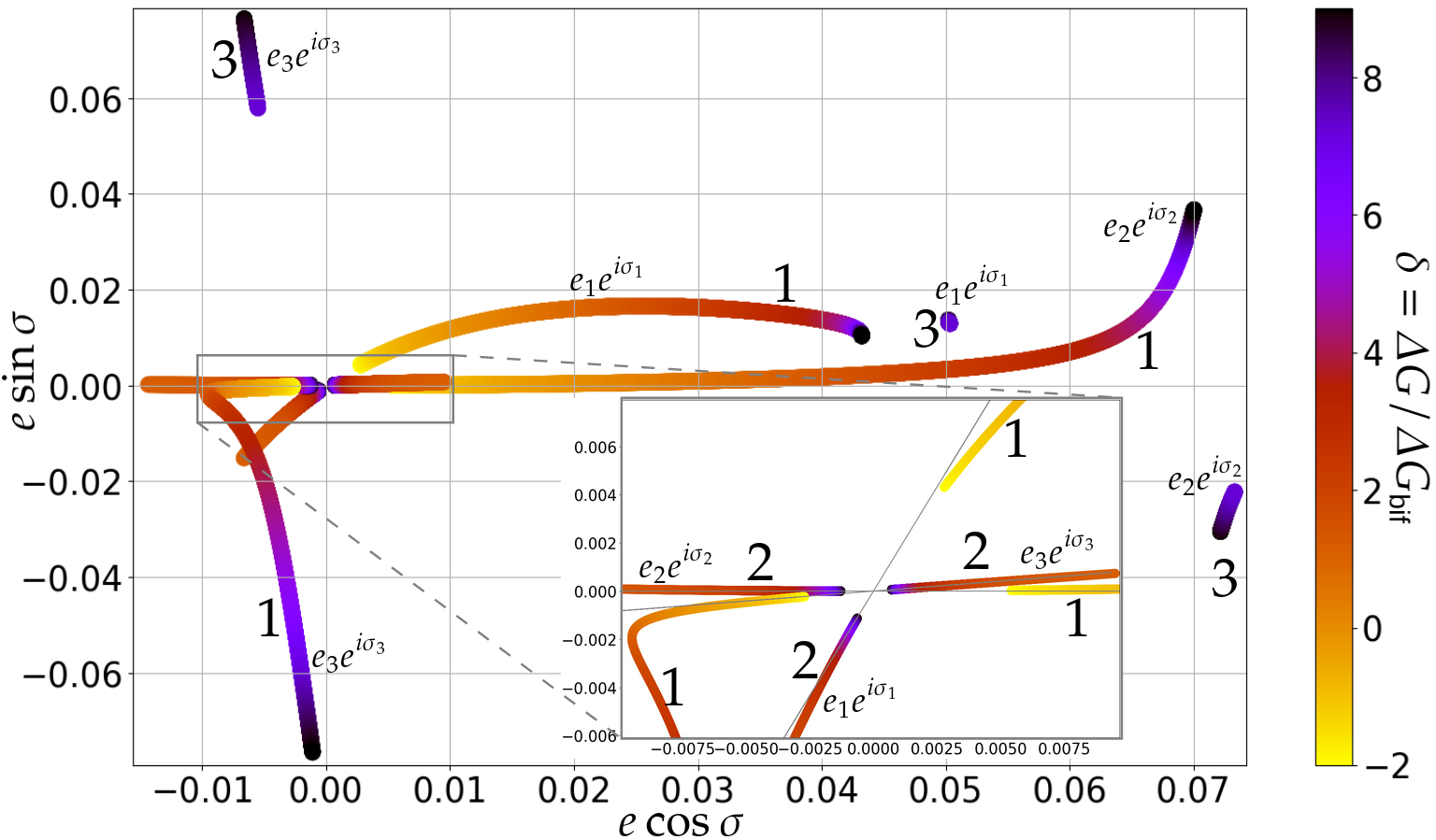
Limiting the work at first order in eccentricity and forcing a decoupling between $\left(L,\xi\right)$ and $\left(D_{j},\sigma_{j}\right)$ gives analytical expressions of the linearised system⁶⁶ 6 At least of the equilibria and the eigenvalues, we did not obtain the eigendirections., but at the cost of strong approximations. We develop here a Newton-Raphson based algorithm to numerically find the equilibria of the model (25) without these approximations.

The vector field $F_{0}$, derived from the Hamiltonian (25), depends on the choice of the parameter $\delta$ (through $\Delta G$) and once a fixed point is found for a particular value of $\delta$, we repeat the Newton-Raphson algorithm for slowly varying values of $\delta$ in order to travel along the whole branch. We look for equilibria exploring the parallelepiped in the phase space defined by $\left|u_{j}\right|<0.08$ and $\left|v_{j}\right|<0.08$ $\left(e_{j}^{2}=C_{j}(u_{j}^{2}+v_{j}^{2})\right)$. We choose $L_{0}=L^{\star}=\Lambda_{1}^{\star}/\Gamma^{\star}$ as initial condition of the Newton-Raphson method for $L$ since all equilibria are expected to be close to this value, and so no discretisation is necessary along this axis. In the same way, we only choose $\xi_{0}\in\left\{\pm\pi/3,\pi\right\}$.

We display in Table 1 all the equilibria that we have found for $\delta=7$, their hyperbolic or elliptic nature, and the value of $\delta$ that gives birth to the branch. Due to the difficulty of exploring a thinly discretised grid in 6 dimensions, we may have not found all the possible equilibria. We discretised the axes $u_{j}$ and $v_{j}$ with only $8$ points, testing $3\times 8^{6}$ initial conditions, all of which converged towards $15$ equilibria. Since the Hamiltonian (25) is invariant by the transformation $(\xi,\sigma_{j})\longmapsto(-\xi,-\sigma_{j})$, fixed points with values of the angles different from $0$ or $\pi$ have a symmetric, hence the $\pm$ and $\mp$ signs in Table 1 (the upper sign corresponds to a fixed point and the lower sign to its symmetric). This symmetry corresponds to the invariance of the system by a rotation of angle $\pi$ around an axis normal to the total angular momentum.

As is seen in Table 1, only the branches $1$, $2$ and $3$ of fixed points can be elliptic, and thus, we focus only on them in the rest of this work. In Fig. 2, we plot these branches for values of $\delta$ ranging from $-2$ to $9$. For branches $1$ and $2$, which are predicted by the first order in eccentricity, we also plot them as given by Eqs. (30) and (35), for comparison. This section shows how the analytical model is unable to locate the equilibria of the simplified Hamiltonian (25) for $e_{j}\gtrsim 0.005$ (see Fig. 2) and does not even give its topology for $e_{j}\gtrsim 0.05$ (see branches $3$, $5$ and $7$ in Table 1, that do not exist at first order in eccentricity). This discrepancy between first and second order in eccentricity was already mentioned by Beaugé et al., 2006 in the case of the two-planet $1:2$ mean motion resonance.

In this section, we compare the position of the equilibria of the secular (simplified) Hamiltonian (25) to that of the corresponding periodic orbits of the complete (full) Hamiltonian (3), that we called libration centres in Sect. 2.2.1. To this aim, we develop an iterative algorithm, similar to what is done by Couetdic et al., 2010, to find a libration centre of the complete Hamiltonian using an equilibrium of the simplified Hamiltonian as initial condition.

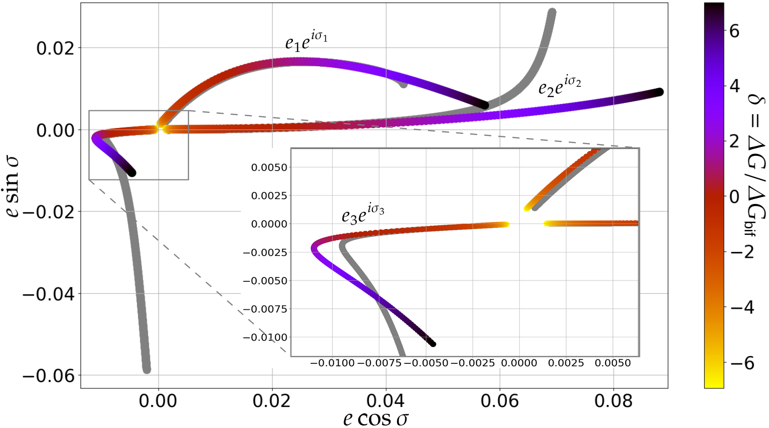
We assume that, close enough to a libration centre of the complete Hamiltonian (3), the trajectories are quasiperiodic, and we write, for any complex quantity $z$ depending on these trajectories,

where the coordinates of $\mathbf{\boldsymbol{\omega}}=\,^{t}\left(\nu,\nu_{2},\nu_{3},g_{1},g_{2},g_{3}\right)$ are the fundamental frequencies of the complete Hamiltonian (3). The frequencies $\nu$, $\nu_{2}$ and $\nu_{3}$ have approximate values given by Eqs. (42), (28) and (33), respectively.

As explained in Sect. 2.2.1, the libration centres correspond to points in the phase space where the motion is periodic⁷⁷ 7 Quasiperiodic with frequencies $\nu_{2}$ and $\nu_{3}$ for a quantity not invariant by rotation around the vertical axis. with frequency $\nu_{2}$.

The description of the algorithm is as follows:

• •

  For a choice of the parameter $\delta$, find the position of an elliptic equilibrium of the simplified Hamiltonian (25) with a Newton-Raphson method. Use it as initial condition to integrate numerically the trajectories of the complete Hamiltonian (3).

• •

  For a complex quantity $z$ depending on the trajectories of (3), obtain the decomposition (43) using a frequency analysis method (Laskar, 1993, e.g.).

• •

  Identify terms depending on frequencies other than $\nu_{2}$ and set to $0$ the corresponding coefficient $z_{\mathbf{\boldsymbol{k}}}$.

• •

  Proceed similarly for different quantities $z$ and evaluate them at time $t=0$ in order to obtain a new initial condition. Restart from the first step using the new initial condition instead of the equilibrium of (25).

The process is iterated until a convergence occurs. In Fig. 3, we display the trajectories of the quantities $e_{j}e^{i\sigma_{j}}$ in the plane $\left(e_{j}\cos\sigma_{j},\,e_{j}\sin\sigma_{j}\right)$, as the algorithm iterates. Isolating terms featuring frequencies other than $\nu_{2}$ is difficult, if not impossible. Indeed, the frequency analysis gives the scalars $\mathbf{\boldsymbol{k}}\cdot\mathbf{\boldsymbol{\omega}}$ but not the vectors $\mathbf{\boldsymbol{k}}$, which cannot be deduced since the vector $\mathbf{\boldsymbol{\omega}}$ is unknown for the complete Hamiltonian. We can get around this difficulty by noticing that $\nu_{2}$ is much larger than the other frequencies, hence it is easy to isolate terms that depend on $\nu_{2}$ from those which do not. The implementation is thus simplified by setting to $0$ the coefficients $z_{\mathbf{\boldsymbol{k}}}$ of the terms that do not depend on $\nu_{2}$.

This algorithm is only able to find libration centres associated with elliptic fixed points. We use it to find the branches of libration centres associated with branches $1$, $2$ and $3$ of Table 1. We confirm the existence of a small hyperbolic zone for branch $2$ in the complete Hamiltonian when the algorithm stops converging as the branch is traveled (by slowly incrementing the value of $\delta$). We plot in Fig. 4 the main branch (branch $1$) of libration centres of the complete Hamiltonian (3) and we compare it with the main branch of equilibria of the simplified Hamiltonian (25). In Fig. 5, we plot the precession frequency of the pericentres, $\nu_{3}$, for the main branch of libration centres, and we compare it with the analytical expression (33). The value of $\nu_{3}$ in the complete Hamiltonian is obtained from the frequency analysis of $e^{i\xi_{3}}$, once the libration centre is known.