NICO⁺⁺: Towards Better Benchmarking for Domain Generalization

Xingxuan Zhang^†, Yue He^†, Renzhe Xu, Han Yu, Zheyan Shen, Peng Cui*
Department of Computer Science, Tsinghua University

xingxuanzhang@hotmail.com, heyue18@mails.tsinghua.edu.cn, xrz199721@gmail.com,
yuh21@mails.tsinghua.edu.cn, shenzy17@mails.tsinghua.edu.cn, cuip@tsinghua.edu.cn

Abstract

²²footnotetext: Equal contribution ¹¹footnotetext: Corresponding Author

Despite the remarkable performance that modern deep neural networks have achieved on independent and identically distributed (I.I.D.) data, they can crash under distribution shifts. Most current evaluation methods for domain generalization (DG) adopt the leave-one-out strategy as a compromise on the limited number of domains. We propose a large-scale benchmark with extensive labeled domains named NICO⁺⁺³³ 3 The dataset can be found at https://www.dropbox.com/sh/u2bq2xo8sbax4pr/AADbhZJAy0AAbap76cg_XkAfa?dl=0. The Github repository for the paper is at https://github.com/xxgege/NICO-plus. along with more rational evaluation methods for comprehensively evaluating DG algorithms. To evaluate DG datasets, we propose two metrics to quantify covariate shift and concept shift, respectively. Two novel generalization bounds from the perspective of data construction are proposed to prove that limited concept shift and significant covariate shift favor the evaluation capability for generalization. Through extensive experiments, NICO⁺⁺ shows its superior evaluation capability compared with current DG datasets and its contribution in alleviating unfairness caused by the leak of oracle knowledge in model selection.

1 Introduction

Machine learning has illustrated its excellent capability in a wide range of areas [Kipf and Welling 2016; Simonyan and Zisserman 2014; Young et al. 2018]. Most current algorithms minimize the empirical risk in training data relying on the assumption that training and test data are independent and identically distributed (I.I.D.). However, this ideal hypothesis is hardly satisfied in real applications, especially those high-stake applications such as healthcare [Castro et al. 2020; Miotto et al. 2018], autonomous driving [Alcorn et al. 2019; Dai and Van Gool 2018; Levinson et al. 2011] and security systems [Berman et al. 2019], owing to the limitation of data collection and intricacy of the scenarios. The distribution shift between training and test data may lead to the unreliable performance of most current approaches in practice. Hence, instead of generalization within the training distribution, the ability to generalize under distribution shift, namely domain generalization (DG) [Wang et al. 2021; Zhou et al. 2021a], is of more critical significance in realistic scenarios.

In the field of computer vision, benchmarks that provide the common ground for competing approaches often play a role of catalyzer promoting the advance of research [Deng et al. 2009]. An advanced DG benchmark should provide sufficient diversity in distributions for both training and evaluating DG algorithms [Xu et al. 2020; Volpi et al. 2018] while ensuring essential common knowledge of categories for inductive inference across domains [Huang et al. 2020; Zhao et al. 2019; Ilse et al. 2020]. The first property drives generalization challenging, and the second ensures the solvability [Ye et al. 2021]. This requires adequate distinct domains and instructive features for each category shared among all domains.

Current DG benchmarks, however, either lack sufficient domains (e.g., 4 domains in PACS [Li et al. 2017], VLCS [Fang et al. 2013] and Office-Home [Venkateswara et al. 2017] and 6 in DomainNet [Peng et al. 2019]) or too simple or limited to simulating significant distribution shifts in real scenarios [Ganin and Lempitsky 2015; Arjovsky et al. 2019; Hendrycks and Dietterich 2019]. To enrich the diversity and perplexing distribution shifts in training data as much as possible, most of the current evaluation methods for DG adopt the leave-one-out strategy, where one domain is considered as test domain and the others for training. This is not an ideal evaluation for generalization but a compromise due to the limited number of domains in current datasets, which impairs the evaluation capability since the model is tested only on one specific distribution instead of multiple unseen distributions every time after training.

To benchmark DG methods comprehensively and simulate real scenarios where a trained model may encounter any possible test data while providing sufficient diversity in the training data, we construct a large-scale DG dataset named NICO⁺⁺ with extensive domains and two protocols supported by aligned and flexible domains across categories, respectively, for better evaluation. Our dataset consists of 80 categories, 10 aligned common domains for all categories, 10 unique domains specifically for each category, and more than 200,000 images. Abundant diversity in both domain and category supports flexible assignments for training and test, controllable degree of distribution shifts, and extensive evaluation on multiple target domains. Images collected from real-world photos and consistency within category concepts provide sufficient common knowledge for recognition across domains on NICO⁺⁺.

To evaluate DG datasets in depth, we investigate distribution shift on images (covariate shift) and common knowledge for category discrimination across domains (concept agreement) within them. Formally, we present quantification for covariate shift and the opposite of concept agreement, namely concept shift, via two novel metrics. We propose two novel generalization bounds and analyze them from the perspective of data construction instead of models. Through these bounds, we prove that limited concept shift and significant covariate shift favor the evaluation capability for generalization.

Moreover, a critical yet common problem in DG is the model selection and the potential unfairness in the comparison caused by leveraging the knowledge of target data to choose hyperparameters that favors test performance [Gulrajani and Lopez-Paz 2021; Arpit et al. 2021]. This issue is exacerbated by the notable variance of test performance with various algorithm irrelevant hyperparameters on current DG datasets. Intuitively, strong and unstable concept shift such as confusing mapping relations from images to labels across domains embarrasses training convergence and enlarges the variance.

We conduct extensive experiments on three levels. First, we evaluate NICO⁺⁺ and current DG datasets with the proposed metrics and show the superiority of NICO⁺⁺ in evaluation capability. Second, we conduct copious experiments on NICO⁺⁺ to benchmark current representative methods with the proposed protocols. Results show that the room for improvement of generalization methods on NICO⁺⁺ is spacious. Third, we show that NICO⁺⁺ helps alleviate the issue by squeezing the possible improvement space of oracle leaking and contributes as a fairer benchmark to the evaluation of DG methods, which meets the proposed metrics.

2 Related Works

In this section, we review the literature related to this paper, including benchmark datasets and domain generalization methods.

Benchmark Datasets.

After the high-speed development benefited from the datasets, like PASCAL VOC [Everingham et al. 2015], ImageNet [Deng et al. 2009] and MSCOCO [Lin et al. 2014], in IID scenarios, a range of image datasets have been raised for the research of domain generalization in visual recognition. The first branch modifies traditional image datasets with synthetic transformations, such as special data selection policies, perturbations or interventions, to simulate distribution shifts, typically including the ImageNet variants [Hendrycks et al. 2021a; Hendrycks and Dietterich 2019; Hendrycks et al. 2021b], MNIST variants [Arjovsky et al. 2019; Ghifary et al. 2015] and Waterbirds [Sagawa et al. 2019]. Another branch considers collecting data coming from different source domains, including PACS [Li et al. 2017], Office-Home [Venkateswara et al. 2017], WILDS [Koh et al. 2021], DomainNet [Peng et al. 2019], Terra Incognita [Beery et al. 2018], NICO [He et al. 2021], and VLCS [Fang et al. 2013]. In specific scenarios, Camelyon17 [Bandi et al. 2018] has tissue slides sampled and post-processed in different hospitals; FMoW [Christie et al. 2018] contains the satellites in distinct time and locations. However, these datasets utilize a simple criterion to distinguish distributions, e.g. image style, not enough to cover the complexity in reality. In addition, the domains of most current DG datasets are limited, leading to inadequate diversity in training or test data. iWildCam [Beery et al. 2021], a large-scale dataset, takes pictures of wild animals with cameras at different locations and produces realistic distributional shifts. But it lacks the ability to control the strength of distribution shift to simulate diverse DG settings. The last version of NICO [He et al. 2021] is insufficient to support some typical settings such as DA and DG since the domains are not aligned across categories.

Domain Generalization.

There are several streams of literature studying the domain generalization problem in vision. With extra information on test domains, domain adaptation methods [Ben-David et al. 2006; Fang et al. 2020; Ghafoorian et al. 2017; Sener et al. 2016; Sugiyama et al. 2007a; Sugiyama et al. 2007b; Tahmoresnezhad and Hashemi 2017; Xu et al. 2021a; Zhang et al. 2016] show effectiveness in addressing the distribution shift problems. By contrast, domain generalization aims to learn models that generalize well on unseen target domains while only data from several source domains are accessible. According to [Shen et al. 2021], DG methods can be divided into three branches, including representation learning [Blanchard et al. 2017; Blanchard et al. 2011; Gan et al. 2016; Grubinger et al. 2015; Jin et al. 2021; Muandet et al. 2013; Nam and Kim 2018; Ghifary et al. 2016; Hu et al. 2020], training strategies [Ding and Fu 2017; Wang et al. 2020; Segu et al. 2020; Mancini et al. 2018; Zhang et al. 2021b; Liao et al. 2020; Carlucci et al. 2019; Ryu et al. 2019; Li et al. 2019; Huang et al. 2020], and data augmentation methods [Yue et al. 2019; Tobin et al. 2017; Peng et al. 2018; Khirodkar et al. 2019; Tremblay et al. 2018; Prakash et al. 2019; Shankar et al. 2018; Volpi et al. 2018; Zhou et al. 2020]. More comprehensive surveys on domain generalization methods can be found in [Wang et al. 2021; Zhou et al. 2021b].

3 NICO⁺⁺: Domain-Extensive Large Scale Domain Generalization Benchmark

In this section, we introduce a novel large-scale domain generalization benchmark NICO⁺⁺, which contains extensive domains and categories. Similar to the original version of NICO [He et al. 2021], each image in NICO⁺⁺ consists of two kinds of labels, namely the category label and the domain label. The category labels correspond to the objective concept (e.g., cat and dog) while the domain labels represent other visual information (e.g., on grass, in water) in the images. To boost the heterogeneity in the dataset to support the thorough evaluation of generalization ability in domain generalization scenarios, we greatly enrich the types of categories and domains and collect a larger amount of images in NICO⁺⁺.

3.1 Constructions of the Category / Domain Labels

We first select 80 categories and then build 10 common and 10 category-specific domains upon them. We provide detailed discussions on the selection of the categories and domains in Appendix.

Categories.

Total 80 categories are provided with a hierarchical structure in NICO⁺⁺. Four broad categories Animal, Plant, Vehicle, and Substance lie on the top level. For each of Animal, Plant, and Vehicle, there exist narrow categories derived from it (e.g., felida and insect belong to Animal) in the middle level. Finally, 80 concrete categories are assigned to their super-category respectively. The hierarchical structure ensures the diversity and balance¹¹ 1 The ratio of the number of categories in Animal, Plant, Vehicle and Substance is $40:12:14:14$ . of categories in NICO⁺⁺, which is vital to simulate realistic domain generalization scenarios in wild environments. Detailed category structure is in Appendix.

Common domains.

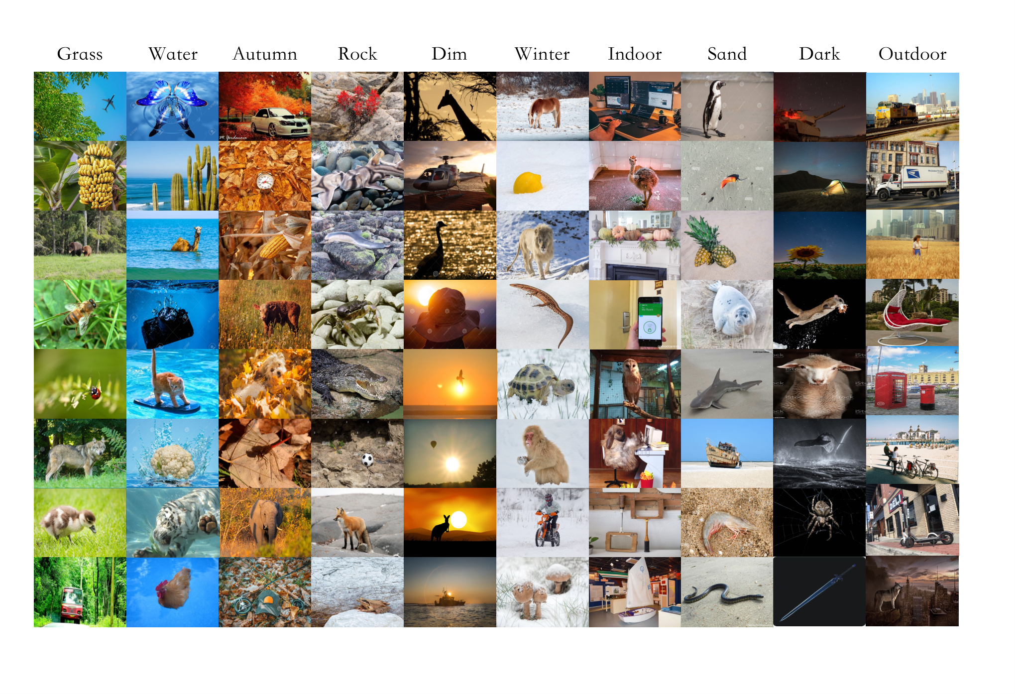
Towards the settings of domain generalization or domain adaption, we design $10$ common domains that are aligned across all categories. Each of the selected common domains refers to a family of concrete contexts with similar semantics so that they are general and common enough to generate meaningful combinations with all categories. For example, the common domain water contains contexts of swimming, in pool, in river, etc. Comparison between common domains in NICO⁺⁺ and domains in current DG datasets is in Appendix.

Unique domains.

To increase the number of domains and support the flexible DG scenarios where the training domains are not aligned with respect to categories, we further attain unique domains specifically for each of the 80 categories. We select the unique domains according to the following conditions: 1) they are different from the common domains; 2) they can include various concepts, such as attributes (e.g. action, color), background, camera shooting angle, and accompanying objects, etc.; 3) different types of them hold a balanced proportion for diversity.

3.2 Data Collection and Statistics

Figure 1: Statistical overview of NICO⁺⁺. The figure shows the number of instances in each domain and each category. The horizontal axis is for categories and the vertical axis for domains. The color of each bin corresponds to the number of instances in each (category, domain) pair. The 10 domains at the bottom are common domains and identical for all categories, while the 10 at the top are unique domains that vary across categories and are represented with {uni_1, uni_1, …, uni_10}.

NICO⁺⁺ has 10 common domains, covering nature, season, humanity and illumination, for total 80 categories, and 10 unique domains for each category. The capacity of most common domains and unique domains is at least 200 and 50, respectively. The images from most domains are collected by searching a combination of a category name and a phrase extend from the domain name (e.g. “dog sitting on grass" for the category dog and the domain grass). Over 32,000 combinations are adopted for searching images. The downloaded data contain a large portion of outliers that require artificial annotations. Each image is assigned to two annotators and passes the selection when agreed by both annotators. After the annotation process, 232.4k images are selected from over 1.0 million images downloaded from the search engines.

The scale of NICO⁺⁺ is enormous enough to support the training of deep convolutional networks (e.g., ResNet-50) from scratch in types of domain generalization scenarios. A statistical overview of the dataset is shown Figure 1.

4 Covariate Shift and Concept Shift

Consider a dataset with data points sampled from a joint distribution $P(X,Y)=P(Y|X)P(X)$ . Distribution shift within the dataset can be caused by the shift on $P(X)$ (i.e., covariate shift) and shift on $P(Y|X)$ (i.e., concept shift) [Shen et al. 2021]. We give quantification for these two shifts in any labeled dataset and analyze the preference of them from a perspective of the DG benckmark via presenting two generalization bounds for multi-class classification. Then we evaluate NICO⁺⁺ and current DG datasets empirically with the proposed metrics and show the superiority of NICO⁺⁺.

Notations

We use $\mathcal{X}$ and $\mathcal{Y}$ to denote the space of input $X$ and outcome $Y$ , respectively. We use $\Delta_{\mathcal{Y}}$ to denote a distribution on $\mathcal{Y}$ . A domain $d$ corresponds to a distribution $\mathcal{D}_{d}$ on $\mathcal{X}$ and a labeling function²² 2 We use $\Delta_{\mathcal{Y}}$ here to denote that the labeling function may not be deterministic. This formulation also includes deterministic labeling function cases. $f_{d}:\mathcal{X}\rightarrow\Delta_{\mathcal{Y}}$ . The training and test domains are specified by $(\mathcal{D}_{{\text{tr}}},f_{{\text{tr}}})$ and $(\mathcal{D}_{\text{te}},f_{\text{te}})$ , respectively. We use $p_{\text{tr}}(x)$ and $p_{\text{te}}(x)$ to denote the probability density function on training and test domains. Let $\ell:\Delta_{\mathcal{Y}}\times\Delta_{\mathcal{Y}}\rightarrow\mathbb{R}_{+}$ define a loss function over $\Delta_{\mathcal{Y}}$ and $\mathcal{H}$ define a function class mapping $\mathcal{X}$ to $\Delta_{\mathcal{Y}}$ . For any hypotheses $h_{1},h_{2}\in\mathcal{H}$ , the expected loss $\mathcal{L}_{\mathcal{D}}(h_{1},h_{2})$ for distribution $\mathcal{D}$ is given as $\mathcal{L}_{\mathcal{D}}(h_{1},h_{2})=\mathbb{E}_{x\sim\mathcal{D}}\left[\ell(h_{1}(x),h_{2}(x))\right]$ . To simplify the notations, we use $\mathcal{L}_{\text{tr}}$ and $\mathcal{L}_{\text{te}}$ to denote the expected loss $\mathcal{L}_{\mathcal{D}_{\text{tr}}}$ and $\mathcal{L}_{\mathcal{D}_{\text{te}}}$ in training and test domain, respectively. In addition, we use $\varepsilon_{{\text{tr}}}(h)=\mathcal{L}_{{\text{tr}}}\left(h,f_{{\text{tr}}}\right)$ and $\varepsilon_{{\text{te}}}(h)=\mathcal{L}_{{\text{te}}}\left(h,f_{{\text{te}}}\right)$ to denote the loss of a function $h\in\mathcal{H}$ w.r.t. to the true labeling function $f_{\text{tr}}$ and $f_{\text{te}}$ , respectively.

4.1 Metrics for Covariate shift and Concept shift

The distribution shift between the training domain $(\mathcal{D}_{\text{tr}},f_{\text{tr}})$ and test domain $(\mathcal{D}_{\text{te}},f_{\text{te}})$ can be decomposed into covariate shift (i.e., shift between $\mathcal{D}_{\text{tr}}$ and $\mathcal{D}_{\text{te}}$ ) and concept shift (i.e., shift between $f_{\text{tr}}$ and $f_{\text{te}}$ ). We propose the following metrics to measure the covariate shift and concept shift.

Definition 4.1 (Metrics for covariate shift and concept shift).

Let $\mathcal{H}$ be a set of functions mapping $\mathcal{X}$ to $\Delta_{\mathcal{Y}}$ and let $\ell:\Delta_{\mathcal{Y}}\times\Delta_{\mathcal{Y}}\rightarrow\mathbb{R}_{+}$ define a loss function over $\Delta_{\mathcal{Y}}$ . For the two domains $(\mathcal{D}_{\text{tr}},f_{\text{tr}})$ and $(\mathcal{D}_{\text{te}},f_{\text{te}})$ , then

–

the covariate shift is measured as the discrepancy distance [Mansour et al. 2009] (provided in Definition 4.2) between $\mathcal{D}_{\text{tr}}$ and $\mathcal{D}_{\text{te}}$ under $\mathcal{H}$ and $\ell$ , i.e.,

\mathcal{M}_{\mathrm{cov}}\left(\mathcal{D}_{\text{tr}},\mathcal{D}_{\text{te}};\mathcal{H},\ell\right)\triangleq\mathrm{disc}\left(\mathcal{D}_{\text{tr}},\mathcal{D}_{\text{te}};\mathcal{H},\ell\right),

(1)

–

the concept shift is measured as the maximum / minimum loss when using $f_{\text{tr}}$ on the test domain or using $f_{\text{te}}$ on the training domain, i.e.,

\left\{\begin{aligned} \mathcal{M}_{\mathrm{cpt}}^{\min}\left(\mathcal{D}_{\text{tr}},\mathcal{D}_{\text{te}},f_{\text{tr}},f_{\text{te}};\ell\right)&\triangleq\min\left\{\mathcal{L}_{{\text{tr}}}(f_{{\text{tr}}},f_{{\text{te}}}),\mathcal{L}_{{\text{te}}}(f_{{\text{tr}}},f_{{\text{te}}})\right\},\\ \mathcal{M}_{\mathrm{cpt}}^{\max}\left(\mathcal{D}_{\text{tr}},\mathcal{D}_{\text{te}},f_{\text{tr}},f_{\text{te}};\ell\right)&\triangleq\max\left\{\mathcal{L}_{{\text{tr}}}(f_{{\text{tr}}},f_{{\text{te}}}),\mathcal{L}_{{\text{te}}}(f_{{\text{tr}}},f_{{\text{te}}})\right\}.\end{aligned}\right.

(2)

Remark.

We introduce two metrics for concept shift terms in Equation 2 because they both provide meaningful characterizations of the concept shift. In addition, both $\mathcal{M}_{\mathrm{cpt}}^{\min}$ and $\mathcal{M}_{\mathrm{cpt}}^{\max}$ have close connections with DG performance as shown in Theorem 4.2 and Theorem 4.3 in Section 4.2. The covariate shift is widely discussed in recent literature [Duchi et al. 2020; Ruan et al. 2021; Shen et al. 2021] yet none of them give the quantification with function discrepancy, which favors the analysis of DG performance and shows remarkable properties when $\mathcal{H}$ is large (such as the function space supported by current deep models). The concept shift can be considered as the discrepancy between the labeling rule $f_{{\text{tr}}}$ on the training data and the labeling rule $f_{{\text{te}}}$ on the test data. Intuitively, consider that a circle in the training data is labeled as class A in training domains and class B in test domains, models can hardly learn the labeling function on the test data (mapping the circle to class B) without knowledge about test domains.

The discrepancy distance mentioned above is defined as follows.

Definition 4.2 (Discrepancy Distance [Mansour et al. 2009]).

Let $\mathcal{H}$ be a set of functions mapping $\mathcal{X}$ to $\Delta_{\mathcal{Y}}$ and let $\ell:\Delta_{\mathcal{Y}}\times\Delta_{\mathcal{Y}}\rightarrow\mathbb{R}_{+}$ define a loss function over $\Delta_{\mathcal{Y}}$ . The discrepancy distance $\mathrm{disc}\left(\mathcal{D}_{1},\mathcal{D}_{2};\mathcal{H},\ell\right)$ between two distributions $\mathcal{D}_{1}$ and $\mathcal{D}_{2}$ over $\mathcal{X}$ is defined by

\mathrm{disc}\left(\mathcal{D}_{1},\mathcal{D}_{2};\mathcal{H},\ell\right)\triangleq\sup_{h_{1},h_{2}\in\mathcal{H}}\left|\mathcal{L}_{\mathcal{D}_{1}}(h_{1},h_{2})-\mathcal{L}_{\mathcal{D}_{2}}(h_{1},h_{2})\right|.

(3)

We give formal analysis of metrics for covariate shift ( $\mathcal{M}_{\mathrm{cov}}$ ) and concept shift ( $\mathcal{M}_{\mathrm{cpt}}^{\min}$ / $\mathcal{M}_{\mathrm{cpt}}^{\max}$ ) below and the graphical explanation is shown in Figure 2.

Refer to caption — Figure 2: Graphical explanations of our proposed metric $\mathcal{M}_{\mathrm{cov}}$ and $\mathcal{M}_{\mathrm{cpt}}^{\min}$ / $\mathcal{M}_{\mathrm{cpt}}^{\max}$ when $\mathcal{H}$ is the set of all functions mapping $\mathcal{X}$ to $\Delta_{\mathcal{Y}}$ and $\ell$ is the 0-1 loss.

The covariate shift term $\mathcal{M}_{\mathrm{cov}}$ .

When the capacity of function class $\mathcal{H}$ is large enough and $\ell$ is bounded, $\mathcal{M}_{\mathrm{cov}}$ is in terms of the $\ell_{1}$ distance between two distributions, given by the following proposition.

Proposition 4.1.

Let $\mathcal{H}$ be the set of all functions mapping $\mathcal{X}$ to $\Delta_{\mathcal{Y}}$ and the range of the loss function is $[0,M]$ , then for any two distributions $\mathcal{D}_{{\text{tr}}}$ and $\mathcal{D}_{\text{te}}$ on $\mathcal{X}$ with probability density function $p_{\text{tr}}$ and $p_{\text{te}}$ respectively,

\mathcal{M}_{\mathrm{cov}}\left(\mathcal{D}_{\text{tr}},\mathcal{D}_{\text{te}};\mathcal{H},\ell\right)=\frac{M}{2}\ell_{1}\left(\mathcal{D}_{\text{tr}},\mathcal{D}_{\text{te}}\right)=\frac{M}{2}\int_{\mathcal{X}}\left|p_{\text{tr}}(x)-p_{\text{te}}(x)\right|\mathrm{d}x.

(4)

It is clear that the covariate shift metric $\mathcal{M}_{\mathrm{cov}}$ is determined by the accumulated bias between the distribution $\mathcal{D}_{{\text{tr}}}$ and $\mathcal{D}_{{\text{te}}}$ defined on $\mathcal{X}$ and without contribution from $\mathcal{Y}$ , which meets the definition of covariate shift.

The concept shift term $\mathcal{M}_{\mathrm{cpt}}^{\min}$ and $\mathcal{M}_{\mathrm{cpt}}^{\max}$ .

When $\ell$ is set as the 0-1 loss, i.e., the loss $\ell(f_{\text{tr}}(x),f_{{\text{te}}}(x))$ is $0$ if and only if $f_{\text{tr}}(x)=f_{\text{te}}(x)$ , $\mathcal{M}_{\mathrm{cpt}}^{\min}$ and $\mathcal{M}_{\mathrm{cpt}}^{\max}$ can be written as follows.

	$\displaystyle\mathcal{M}_{\mathrm{cpt}}^{\min}$	$\displaystyle=\min\left\{\int_{\mathcal{X}}\mathbb{I}[f_{{\text{tr}}}(x)\neq f_{{\text{te}}}(x)]p_{{\text{tr}}}(x)\mathrm{d}x,\int_{\mathcal{X}}\mathbb{I}[f_{{\text{tr}}}(x)\neq f_{{\text{te}}}(x)]p_{{\text{te}}}(x)\mathrm{d}x\right\}$		(5)
	$\displaystyle\mathcal{M}_{\mathrm{cpt}}^{\max}$	$\displaystyle=\max\left\{\int_{\mathcal{X}}\mathbb{I}[f_{{\text{tr}}}(x)\neq f_{{\text{te}}}(x)]p_{{\text{tr}}}(x)\mathrm{d}x,\int_{\mathcal{X}}\mathbb{I}[f_{{\text{tr}}}(x)\neq f_{{\text{te}}}(x)]p_{{\text{te}}}(x)\mathrm{d}x\right\}$		(5)

Here $\mathbb{I}[f_{\text{tr}}(x)\neq f_{\text{te}}(x)]$ is an indicator function on whether $f_{\text{tr}}(x)\neq f_{\text{te}}(x)$ . Intuitively, the two terms in the $\min$ / $\max$ functions represent the probabilities of inconsistent labeling function in training and test domains. $\mathcal{M}_{\mathrm{cpt}}^{\min}$ and $\mathcal{M}_{\mathrm{cpt}}^{\max}$ further take the minimal and maximal value of the two probabilities, respectively. It is rational that the concept shift is actually the integral of $p_{{\text{tr}}}(x)$ (or $p_{{\text{te}}}(x)$ ) over any points $x$ where its corresponding label on training data differs from that on test data. In practice, we estimate $f_{{\text{tr}}}$ and $f_{{\text{te}}}$ with models trained on source domains and target domains, respectively. More discussion and comparison of discrepancy distance and other metrics for distribution distance is in Appendix.

4.2 Dataset Evaluation with the Metrics

To use the covariate shift metric $\mathcal{M}_{\mathrm{cov}}$ and concept shift metrics $\mathcal{M}_{\mathrm{cpt}}^{\min},\mathcal{M}_{\mathrm{cpt}}^{\max}$ for dataset evaluation, we show that larger covariate shift and smaller concept shift favors a discriminative domain generalization benchmark. Intuitively, the critical point of datasets for domain generalization lies in 1) significant covariate shift between domains that drives generalization challenging [Quiñonero-Candela et al. 2008] and 2) common knowledge about categories across domains on which models can rely on to conduct valid predictions on unseen domains [Zhao et al. 2019; Ilse et al. 2020]. The common knowledge requires the alignment between labeling functions of source domains and target domains, i.e., a moderate concept shift. When there is a strong inconsistency between labeling rules on training and test data, the classification loss instructing biased connections between visual features and concepts is misleading for generalization to test data. Thus models can hardly learn strong predictors for test data without knowledge of test domain.

To analyze the intuitions theoretically, we first propose an upper bound for the expected loss in the test domain for any hypothesis $h\in\mathcal{H}$ .

Theorem 4.2.

Suppose the loss function $\ell$ is symmetric and obeys the triangle inequality. Suppose $f_{{\text{tr}}},f_{{\text{te}}}\in\mathcal{H}$ . Then for any hypothesis $h\in\mathcal{H}$ , the following holds

\varepsilon_{{\text{te}}}(h)\leq\varepsilon_{{\text{tr}}}(h)+\mathcal{M}_{\mathrm{cov}}\left(\mathcal{D}_{\text{tr}},\mathcal{D}_{\text{te}};\mathcal{H},\ell\right)+\mathcal{M}_{\mathrm{cpt}}^{\min}\left(\mathcal{D}_{\text{tr}},\mathcal{D}_{\text{te}},f_{\text{tr}},f_{\text{te}};\ell\right).

(6)

Remark.

Theorem 4.2 is closely related to generalization bounds in domain adaptation (DA) literature [Ben-David et al. 2006; Zhang et al. 2019; Zhao et al. 2019; Zhang et al. 2020]. In detail, [Ben-David et al. 2006] first studied the generalization bound from a source domain to a target domain in binary classification problems and [Zhang et al. 2019; Zhang et al. 2020] further extended the results to multi-class classification problems. However, the bounds in their results depend on a specific term $\lambda^{*}\triangleq\min_{h\in\mathcal{H}}\varepsilon_{{\text{tr}}}(h)+\varepsilon_{{\text{te}}}(h)$ , which is conservative and relatively loose and can not be measured as concept shift directly [Zhao et al. 2019]. As a result, [Zhao et al. 2019] developed a bound which explicitly takes concept shift (termed as conditional shift by them) into account. However, their results are only applied to binary classifications and $\ell_{1}$ loss function. By contrast, Theorem 4.2 can be applied to multi-class classifications problems and any loss functions that are symmetric and obeys the triangle inequality.

Theorem 4.2 quantitatively gives an estimation about the biggest gap between the performance of a model on training and test data. If we consider $\mathcal{H}$ as a set of deep models trained on training data with different learning strategies, the estimation indicates the upper bound of range in which their performance varies. If we consider $h$ as a model that fits training data, the bound gives an estimation of how much the distribution shift of the dataset contributes to the performance drop between training and test data.

Furthermore, we propose a lower bound for the expected loss in the test domain for any hypothesis $h\in\mathcal{H}$ to better understand how the proposed metrics $\mathcal{M}_{\mathrm{cpt}}$ and $\mathcal{M}_{\mathrm{cov}}$ affects discrimination ability of datasets.

Theorem 4.3.

\displaystyle\varepsilon_{{\text{te}}}(h)\geq\mathcal{M}_{\mathrm{cpt}}^{\max}\left(\mathcal{D}_{\text{tr}},\mathcal{D}_{\text{te}},f_{\text{tr}},f_{\text{te}};\ell\right)-\mathcal{M}_{\mathrm{cov}}\left(\mathcal{D}_{\text{tr}},\mathcal{D}_{\text{te}};\mathcal{H},\ell\right)-\varepsilon_{{\text{tr}}}(h).

(7)

As shown in Theorem 4.3, for any hypothesis $h\in\mathcal{H}$ , the term ( $\mathcal{M}_{\mathrm{cpt}}-\mathcal{M}_{\mathrm{cov}}$ ) determines the lower bound of the test loss and further determines the upper bound of the test performance of $h$ . The bound is critical to evaluate a dataset since the performance of any well-trained model on test data is upper bounded by the properties (concept shift and covariate shift) of the dataset, disregarding how the model is designed or learned. Specifically, consider the stop training condition of a any possible model $h$ is that the loss on the training data is smaller than $\gamma$ , which is rational with most of current training strategies, the performance of the model on test data is upper bounded by $\gamma-\mathcal{M}_{\mathrm{cpt}}+\mathcal{M}_{\mathrm{cov}}$ , which is irrelevant to the choice of $h$ and the learning protocol. Intuitively, when the discrepancy between labeling functions between training and test data, the better the model fits training data, the worse it generalizes to test domains. Conversely, with more aligned labeling functions, the common knowledge between training and test data is richer and more instructive, so that the ceiling of generalization is higher. Moreover, the covariate shift $\mathcal{M}_{\mathrm{cov}}$ contributes positively to the upper bound of the test performance, given that the concept shift $\mathcal{M}_{\mathrm{cpt}}$ can be considered as integral of probability density $p_{{\text{tr}}}(x)$ (or $p_{{\text{te}}}(x)$ ) over points with unaligned labeling functions, where the covariate shift $\mathcal{M}_{\mathrm{cov}}$ helps to counteract the impact of labeling mismatch.

As a result, the drop given by Theorem 4.3 is unsolvable for algorithms but modifiable by suppressing the concept shift or enhancing the covariate shift. To better evaluate generalization ability, an DG benchmark requires small concept shift and large covariate shift. The empirical versions of Theorem 4.2 and Theorem 4.3 are provided in Appendix.

4.3 Empirical Evaluation

Table 1: Results of estimated covariate shift and concept shift of NICO⁺⁺ and current DG datasets.

\uparrow

donates that the higher the metric is, the better and

\downarrow

is the opposite. The best results of all datasets are highlighted with the bold font.

	I.I.D.	PACS	DomainNet	VLCS	Office-Home	MNIST-M	NICO⁺⁺
$\mathcal{M}_{\mathrm{cov}}\uparrow$	0	0.325( $\pm$ 0.053)	0.302( $\pm$ 0.039)	0.256( $\pm$ 0.041)	0.238( $\pm$ 0.049)	0.225( $\pm$ 0.034)	0.338( $\pm$ 0.031)
$\mathcal{M}_{\mathrm{cpt}}^{\min}\downarrow$	0	0.434( $\pm$ 0.023)	0.247( $\pm$ 0.055)	0.303( $\pm$ 0.064)	0.353( $\pm$ 0.086)	0.243( $\pm$ 0.048)	0.152( $\pm$ 0.034)
$\mathcal{M}_{\mathrm{cpt}}^{\max}\downarrow$	0	0.537( $\pm$ 0.054)	0.612( $\pm$ 0.057)	0.523( $\pm$ 0.044)	0.505( $\pm$ 0.084)	0.449( $\pm$ 0.030)	0.192( $\pm$ 0.040)

We compare NICO⁺⁺ with current DG datasets in both covariate shift $\mathcal{M}_{\mathrm{cov}}$ and concept shift $\mathcal{M}_{\mathrm{cpt}}^{\min}$ , $\mathcal{M}_{\mathrm{cpt}}^{\max}$ .

For the covariate shift term, we first train two models from scratch jointly by optimizing the following two objective function, namely

\mathcal{L}_{\mathrm{disc}}^{(1)}=\mathcal{L}_{\mathcal{D}_{\text{tr}}}(h_{1},h_{2})-\mathcal{L}_{\mathcal{D}_{\text{te}}}(h_{1},h_{2}),\quad\mathcal{L}_{\mathrm{disc}}^{(2)}=\mathcal{L}_{\mathcal{D}_{\text{tr}}}(h_{1},h_{2})-\mathcal{L}_{\mathcal{D}_{\text{te}}}(h_{1},h_{2}).

(8)

We take the bigger one of the absolute value of $\mathcal{L}_{\mathrm{disc}}^{(1)}$ and $\mathcal{L}_{\mathrm{disc}}^{(2)}$ as the final indicator for covariate shift $\mathcal{M}_{\mathrm{cov}}$ . We adopt raw ResNet50 [He et al. 2016] as the model for NICO⁺⁺, PACS, DomainNet, VLCS, and Office-Home and shallower CNNs (the structure is shown in Appendix) for MNIST-M [Ganin and Lempitsky 2015] as its image size is small. For a fair comparison, we randomly select 2 domains as the source and 2 domains as the target for all datasets. Since there are only 5 categories in VLCS, we randomly select 5 categories from each domain for each run and report the average of 5 runs. Source and target domains from different datasets are set to approximately the same capacity of images. The learning rate for all models is set to 0.1, batch size is 64, and the number of training epoch is 20.

For the concept shift, we estimate $f_{{\text{tr}}}$ and $f_{{\text{te}}}$ with models that fit the source set and target set, respectively. Specifically, we learn two models on the source and target set of a given dataset, respectively, with the objective of category recognition and each of them on both source and target data. More details of implementation can be found in Appendix.

Results are shown in Table 1. Concept shift on NICO⁺⁺ is significantly lower than other datasets, indicating more aligned labeling rules across domains and more instructive common knowledge of categories can be learned by models. The covariate shifts of NICO⁺⁺, PACS, and DomainNet are comparable, which demonstrates that the distribution shift on images caused by the background can be as strong as style shifts. It is worthy to notice that the term $\mathcal{M}_{\mathrm{cpt}}-\mathcal{M}_{\mathrm{cov}}$ in Theorem 4.3 is larger than 0 on current DG datasets while lower than 0 on NICO⁺⁺, indicating that the drop caused by a shift of labeling function across domains is significant enough to damage the upper generalization bound while the common knowledge across domains in NICO⁺⁺ is sufficient for models to approach the oracle performance.

5 Experiments

Inspired by [Zhang et al. 2021a], we present two evaluation settings, namely classic domain generalization and flexible domain generalization and perform extensive experiments on both settings. We design experimental settings to evaluate current DG methods on NICO⁺⁺ and illustrate how NICO⁺⁺ contributes to filling in the evaluation on generalization to multiple unseen domains. Due to space limitations, we only report major results, and more experiments and implementation details are provided in Appendix.

5.1 Evaluation Metrics for Algorithms

Despite the fact that the widely adopted evaluation methods in DG effectively shows the generalization ability of models to the unseen target domain, they fail to sufficiently simulate real scenarios in application. For example, the most popular evaluation method, namely leave-one-out evaluation [Li et al. 2017; Shen et al. 2021], tests models on a single target domain for each training process, while in real applications, a trained model is required to be reliable under any possible scenarios with various data distributions. The compromise on the limitation of domain numbers in current benchmarks, including PACS, VLCS, DomainNet, Office-Home, can be addressed by NICO⁺⁺ with sufficient aligned and unique domains. The superiority supports designing more realistic evaluation metrics to test models’ generalization ability comprehensively.

We consider three simple metrics to evaluate DG algorithm, namely average accuracy, overall accuracy, and the standard deviation of accuracy across domains. The metrics are defined as follows.

		$\displaystyle\mathrm{Average}=\frac{1}{K}\sum_{k=1}^{K}\mathrm{acc}_{k},\quad\mathrm{Overall}=\frac{1}{\sum_{k=1}^{K}N_{k}}\sum_{k=1}^{K}N_{k}\mathrm{acc}_{k},$		(9)
		$\displaystyle\mathrm{Std}=\sqrt{\frac{1}{K-1}\sum_{k=1}^{K}(\mathrm{acc}_{k}-\mathrm{Average})^{2}}.$		(9)

Here $K$ is the number of domains in the test data, $N_{k}$ is the number of samples in the $k$ -th domain, and $\mathrm{acc}_{k}$ is the prediction accuracy in the $k$ -th domain. The metric $\mathrm{Average}$ is widely used in the literature of DG, where both training and test domains for different categories are aligned. The metric $\mathrm{Overall}$ is more reasonable when the domains can be various for different categories or the test data are a mixture of unknown domains, and thus the accuracy for each domain is incalculable. The metric $\mathrm{Std}$ indicates the standard deviation of the performance across different domains. Since learning models that are consistently reliable in any possible environment is the target of DG and many methods are designed to learn invariant representations [Ganin et al. 2016], $\mathrm{Std}$ is rational and instructive. Please note that $\mathrm{Std}$ is insignificant in the leave-one-out evaluation method where models tested on different target domains are trained on different combinations of source domains, while domains of NICO⁺⁺ are rich enough to evaluate models on various target domains with fixed source domains.

5.2 Benchmark for Classic Domain Generalization

The common domains in NICO⁺⁺ are consistent for all categories, which supports the experimental designs of DG with aligned domains. They can be further grouped into 3 clusters with respect to the kind of distribution shift (detailed discussions are in Appendix), namely location (e.g., indoor or outdoor), background (e.g., around water or on grass), and time (e.g., dim or dark, winter or autumn) shift. In this section we consider two levels of distribution shift, where domains across clusters are selected for test and domains within the same cluster for test, respectively. Six domains are selected for training and the others for test and the results of current representative methods with ResNet-50 as the backbone are shown in Table 2. Models generally show better generalization when tested on a single cluster of common domains than the opposite, indicating that generalization to diverse unseen domains is more challenging. Current SOTA methods such as EoA, CORAL, and StableNet show their effectiveness, yet a significant gap between them and the oracle performance shows that the room for improvement is spacious. More splits and implementation details are in Appendix.

Table 2: Results of the DG setting on NICO⁺⁺. We report the accuracy on each target domain, overall accuracy, mean accuracy, and variance of accuracies across all target domains. We reimplement state-of-the-art unsupervised methods on DomainNet with ResNet-50 [He et al. 2016] as the backbone network for all the methods unless otherwise specified. Oracle donates the ResNet-50 trained with data sampled from the target distribution (yet none of test images is seen in the training). Ova. and Avg. indicate the overall accuracy of all the test data and the arithmetic mean of the accuracy of 3 domains, respectively. Note that they are different because the capacities of different domains are not equal. The reported results are average over three repetitions of each run. The best results of all methods are highlighted with the bold font and the second best with underlined font.

Method	Training domains: G, Wa, R, A, I, Di							Training domains: S, G, Wa, R, I, O
Method	S	Wi	O	Da	Ova.	Avg.	Std	A	Wi	Da	Di	Ova.	Avg.	Std
Deepall	80.95	79.96	73.30	76.27	77.50	77.62	3.05	81.47	79.53	78.13	77.19	79.20	79.08	1.61
SWAD [Cha et al. 2021]	82.71	81.92	76.15	77.20	79.54	79.50	2.86	82.95	80.33	79.16	77.58	79.82	80.00	1.96
MMLD [Matsuura and Harada 2020]	76.45	80.11	76.25	76.91	77.40	77.43	1.57	80.25	78.27	78.56	76.23	78.15	78.33	1.43
RSC [Huang et al. 2020]	80.07	80.22	76.67	76.14	78.37	78.27	1.88	81.22	80.61	78.45	77.60	79.42	79.47	1.49
AdaClust [Thomas et al. 2021]	79.57	78.53	71.75	74.91	76.06	76.19	3.09	80.40	78.63	76.53	75.82	77.96	77.85	1.80
SagNet [Nam et al. 2021]	80.31	79.24	72.97	75.84	76.96	77.09	2.90	80.85	79.11	77.50	76.56	78.63	78.51	1.63
EoA [Arpit et al. 2021]	82.30	81.63	75.02	78.83	79.32	79.45	2.87	82.88	81.14	79.57	79.10	80.76	80.67	1.48
Mixstyle [Zhou et al. 2021b]	80.74	79.59	73.80	76.39	77.51	77.63	2.73	81.02	79.20	77.67	77.25	78.87	78.78	1.48
MLDG [Li et al. 2018a]	81.46	80.28	73.73	76.92	77.96	78.10	3.02	81.88	79.95	78.74	77.79	79.71	79.59	1.53
MMD [Li et al. 2018b]	81.37	80.63	73.82	77.10	78.12	78.23	3.01	81.93	80.28	78.71	77.85	79.81	79.69	1.56
CORAL [Sun and Saenko 2016]	82.66	81.36	74.70	78.25	79.09	79.24	3.07	82.84	81.08	79.49	78.82	80.67	80.56	1.55
StableNet [Zhang et al. 2021a]	81.52	80.36	76.17	77.29	78.85	78.84	2.18	82.56	82.21	78.35	77.46	80.12	80.15	2.27
FACT [Xu et al. 2021b]	80.83	79.66	76.30	78.05	78.61	78.71	1.71	81.37	79.39	78.06	78.58	79.37	79.35	1.26
JiGen [Carlucci et al. 2019]	81.67	80.36	76.54	78.17	79.08	79.18	1.98	81.64	79.84	78.14	78.89	79.63	79.63	1.31
GroupDRO [Sagawa et al. 2019]	81.08	79.92	73.39	76.58	77.61	77.74	3.01	81.35	79.50	78.14	77.23	79.17	79.05	1.55
IRM [Arjovsky et al. 2019]	70.59	72.02	61.83	69.28	68.33	68.43	3.93	72.96	71.52	67.31	69.43	70.25	70.31	2.14
Oracle	86.42	86.68	84.44	84.59	85.55	85.53	1.02	87.79	87.86	84.33	85.18	86.29	86.29	1.57

5.3 Benchmark for Flexible Domain Generalization

Compared current DG setting where domains are aligned across categories, flexible combination of categories and domains in both training and test data can be more realistic and challenging [Zhang et al. 2021a; Shen et al. 2021]. In such cases, the level of the distribution shifts varies in different classes, requiring a strong ability of generalization to tell common knowledge of categories from various domains. We present two settings, namely random and compositional. We randomly select two domains out of common domains as dominant ones, 12 out of the remaining domains as minor ones and the other 6 domains as test data for each category for the random setting. There can be spurious correlations between domains and labels since a domain can be with class A in training data and class B in test data, while there can not be with class A in both training and test data. For the compositional setting, 4 domains are chosen as exclusive training domains and others as sharing domains. Then 2 domains are randomly selected from exclusive training domains as majority, 12 from sharing domains as minority and the remaining 4 in sharing domains for test. Thus there is no spurious correlations between dominant domains and labels. We select all images from dominant domains and 50 images from each minor domain for training and 50 images from each test domain for test. Results are shown in Table 3. Current SOTA algorithm outperforms ERM by a noticeable margin, yet the gap to Oracle remains significant. More splits, discussions and implementation details are in Appendix.

Table 3: Results of the flexible DG setting on NICO⁺⁺.

Method	Deepall	SWAD	MMLD	RSC	AdaClust	SagNet	EoA	MixStyle	StableNet	FACT	JiGen	Oracle
Rand.	74.19	75.62	73.25	75.20	73.39	72.79	76.22	73.47	77.37	75.34	75.44	84.60
Comp.	78.01	76.97	76.85	75.76	76.64	76.15	79.62	77.01	78.19	79.39	78.77	86.18
Avg.	76.10	76.30	75.05	75.48	75.02	74.47	77.92	75.24	77.78	77.37	77.11	85.39

Table 4: Standard deviation across epochs and seeds on different datasets.

	PACS			DomainNet			VLCS			OfficeHome			NICO⁺⁺
Method	Epoch	Seed	Gap	Epoch	Seed	Gap	Epoch	Seed	Gap	Epoch	Seed	Gap	Epoch	Seed	Gap
Deepall	0.96	0.82	2.66	0.61	0.57	0.46	0.83	0.58	3.59	0.77	0.59	0.81	0.22	0.10	0.39
SWAD	0.41	0.76	1.61	0.35	0.30	0.39	0.74	0.49	0.58	0.31	0.25	0.30	0.07	0.05	0.06
MMLD	1.68	2.02	3.25	1.03	0.50	0.85	2.33	1.12	3.97	1.25	0.47	0.56	0.25	0.10	0.15
RSC	0.76	0.81	0.93	0.55	0.35	0.56	1.02	0.61	0.80	0.85	0.37	0.89	0.18	0.05	0.10
AdaClust	1.06	1.74	1.54	0.98	0.41	0.72	1.32	1.79	1.34	1.36	1.30	0.28	0.22	0.04	0.13
SagNet	0.74	2.44	2.78	0.92	0.23	0.54	0.94	1.74	4.19	0.80	0.30	0.44	0.11	0.31	0.61
EoA	0.11	0.36	0.18	0.22	0.16	0.02	0.15	0.45	0.21	0.05	0.29	0.08	0.02	0.04	0.13
MixStyle	1.53	0.63	1.69	0.60	0.36	0.42	1.27	1.78	3.40	0.72	0.43	0.56	0.17	0.16	0.00
MLDG	0.82	1.02	1.24	0.53	0.25	0.55	1.15	1.01	4.14	1.03	0.09	0.23	0.10	0.08	0.12
MMD	1.13	2.39	0.66	0.82	0.24	0.50	1.98	1.32	3.72	0.61	0.02	1.34	0.11	0.11	0.16
CORAL	1.09	1.02	1.18	0.52	0.48	0.47	0.77	0.94	3.18	0.49	0.28	0.50	0.06	0.17	0.19
StableNet	0.90	1.25	1.03	0.34	0.71	0.82	0.86	0.69	0.88	0.44	0.21	0.48	0.09	0.05	0.09
FACT	0.31	0.46	0.52	0.14	0.16	0.37	0.64	0.85	1.17	0.21	0.27	0.68	0.06	0.19	1.09
JiGen	0.33	1.15	0.70	0.16	0.18	0.39	0.51	0.67	1.30	0.20	0.69	0.25	0.05	0.09	0.10
GroupDRO	1.27	0.96	2.09	0.96	0.37	0.54	1.18	0.85	4.93	0.63	0.47	0.55	0.16	0.10	0.16
IRM	3.77	3.02	4.14	2.17	0.89	0.00	6.00	1.74	5.77	2.10	1.59	0.00	0.90	0.54	0.00

5.4 Test Variance and Model Selection

Model selection (including the choice of hyperparameters, training checkpoints and architecture variants) effects DG evaluation considerably [Arpit et al. 2021; Gulrajani and Lopez-Paz 2021; Shen et al. 2021]. The leak of knowledge of test data in training or model selection phase is criticized yet still usual in current algorithms [Gulrajani and Lopez-Paz 2021; Arpit et al. 2021]. This issue is exacerbated by the variance of test performance across random seeds, training iterations and other hyperparameters in that one can choose the best seed or the model from the best epoch under the guidance of released oracle validation set for a noticeable improvement. NICO⁺⁺ presents a feasible approach by reducing the test variance and thus decreasing the possible improvement by leveraging the leak.

As shown in Section 4, the gap between the performance of a model on training and test data is bounded by the sum of covariant shift and concept shift between source and target domains. Intuitively, test variance on NICO⁺⁺ is lower than other current DG datasets given that NICO⁺⁺ guarantees a significantly lower concept shift. Strong concept shift between source domains introduces confusing mapping relations between input $\mathrm{X}$ and output $\mathrm{Y}$ , embarrassing the convergence and enlarging the variance. Since most current deep models are optimized by stochastic gradient descent (SGD), the test accuracy is prone to jitter as the input sequence determined by random seeds varies. Moreover, concept shift also grows the mismatch between the performance on validation data and test data, further widening the gap between target guided and source guided model selection.

Empirically, we compare the test variance and the improvement of leveraging oracle knowledge on NICO⁺⁺ with other datasets across various seeds and training epochs in Table 4. For the test variance across random seeds, we train 3 models for each method with 3 random seeds and calculate the test variance among them. For the test variance across epochs, we calculate the test variance of the models saved on the last 10 epochs for each random seed and show the mean value of 3 random seeds. NICO⁺⁺ shows a lower test variance compared with other datasets across both various random seeds and training epochs, indicating a more stable estimation of generalization ability robust to the choice of algorithm irrelevant hyperparameters. As a result, NICO⁺⁺ alleviates the oracle leaking issue by significantly squeezing the possible improvement space, leading to a fairer comparison for DG methods.

6 Conclusion

In this paper, we investigated the common grounds of advanced approaches for domain generalization in vision. To facilitate the progressive research, we proposed a context-extensive large-scale benchmark named NICO⁺⁺ along with more rational evaluation methods for comprehensively evaluating DG algorithms. Two metrics to quantify covariate shift and concept shift are proposed to evaluate DG datasets upon two novel generalization bounds. Extensive experiments showed the superiority of NICO⁺⁺ over current datasets and benchmarked DG algorithms comprehensively.

References

Alcorn et al. [2019] Michael A Alcorn, Qi Li, Zhitao Gong, Chengfei Wang, Long Mai, Wei-Shinn Ku, and Anh Nguyen. Strike (with) a pose: Neural networks are easily fooled by strange poses of familiar objects. In Proceedings of the IEEE/CVF Conference on Computer Vision and Pattern Recognition, pages 4845–4854, 2019.
Arjovsky et al. [2019] Martin Arjovsky, Léon Bottou, Ishaan Gulrajani, and David Lopez-Paz. Invariant risk minimization. arXiv preprint arXiv:1907.02893, 2019.
Arpit et al. [2021] Devansh Arpit, Huan Wang, Yingbo Zhou, and Caiming Xiong. Ensemble of averages: Improving model selection and boosting performance in domain generalization. arXiv preprint arXiv:2110.10832, 2021.
Bai et al. [2020] Haoyue Bai, Rui Sun, Lanqing Hong, Fengwei Zhou, Nanyang Ye, Han-Jia Ye, S-H Gary Chan, and Zhenguo Li. Decaug: Out-of-distribution generalization via decomposed feature representation and semantic augmentation. arXiv preprint arXiv:2012.09382, 2020.
Bandi et al. [2018] Peter Bandi, Oscar Geessink, Quirine Manson, Marcory Van Dijk, Maschenka Balkenhol, Meyke Hermsen, Babak Ehteshami Bejnordi, Byungjae Lee, Kyunghyun Paeng, Aoxiao Zhong, et al. From detection of individual metastases to classification of lymph node status at the patient level: the camelyon17 challenge. IEEE transactions on medical imaging, 38(2):550–560, 2018.
Bartlett and Mendelson [2002] Peter L Bartlett and Shahar Mendelson. Rademacher and gaussian complexities: Risk bounds and structural results. Journal of Machine search, 3(Nov):463–482, 2002.
Beery et al. [2018] Sara Beery, Grant Van Horn, and Pietro Perona. Recognition in terra incognita. In Proceedings of the European conference on computer vision (ECCV), pages 456–473, 2018.
Beery et al. [2021] Sara Beery, Arushi Agarwal, Elijah Cole, and Vighnesh Birodkar. The iwildcam 2021 competition dataset. arXiv preprint arXiv:2105.03494, 2021.
Ben-David et al. [2006] Shai Ben-David, John Blitzer, Koby Crammer, and Fernando Pereira. Analysis of representations for domain adaptation. Advances in neural information processing systems, 19, 2006.
Berman et al. [2019] Daniel S Berman, Anna L Buczak, Jeffrey S Chavis, and Cherita L Corbett. A survey of deep learning methods for cyber security. Information, 10(4):122, 2019.
Blanchard et al. [2011] Gilles Blanchard, Gyemin Lee, and Clayton Scott. Generalizing from several related classification tasks to a new unlabeled sample. NeurIPS, 24:2178–2186, 2011.
Blanchard et al. [2017] Gilles Blanchard, Aniket Anand Deshmukh, Urun Dogan, Gyemin Lee, and Clayton Scott. Domain generalization by marginal transfer learning. arXiv preprint arXiv:1711.07910, 2017.
Carlucci et al. [2019] Fabio M Carlucci, Antonio D’Innocente, Silvia Bucci, Barbara Caputo, and Tatiana Tommasi. Domain generalization by solving jigsaw puzzles. In Proceedings of the IEEE/CVF Conference on Computer Vision and Pattern Recognition, pages 2229–2238, 2019.
Castro et al. [2020] Daniel C Castro, Ian Walker, and Ben Glocker. Causality matters in medical imaging. Nature Communications, 11(1):1–10, 2020.
Cha et al. [2021] Junbum Cha, Sanghyuk Chun, Kyungjae Lee, Han-Cheol Cho, Seunghyun Park, Yunsung Lee, and Sungrae Park. Swad: Domain generalization by seeking flat minima. Advances in Neural Information Processing Systems, 34, 2021.
Christie et al. [2018] Gordon Christie, Neil Fendley, James Wilson, and Ryan Mukherjee. Functional map of the world. In Proceedings of the IEEE Conference on Computer Vision and Pattern Recognition, pages 6172–6180, 2018.
Dai and Van Gool [2018] Dengxin Dai and Luc Van Gool. Dark model adaptation: Semantic image segmentation from daytime to nighttime. In 2018 21st International Conference on Intelligent Transportation Systems (ITSC), pages 3819–3824. IEEE, 2018.
Deng et al. [2009] Jia Deng, Wei Dong, Richard Socher, Li-Jia Li, Kai Li, and Li Fei-Fei. Imagenet: A large-scale hierarchical image database. In 2009 IEEE conference on computer vision and pattern recognition, pages 248–255. Ieee, 2009.
Ding and Fu [2017] Zhengming Ding and Yun Fu. Deep domain generalization with structured low-rank constraint. IEEE Transactions on Image Processing, 27(1):304–313, 2017.
Duchi et al. [2020] John Duchi, Tatsunori Hashimoto, and Hongseok Namkoong. Distributionally robust losses for latent covariate mixtures. arXiv preprint arXiv:2007.13982, 2020.
Everingham et al. [2015] Mark Everingham, SM Eslami, Luc Van Gool, Christopher KI Williams, John Winn, and Andrew Zisserman. The pascal visual object classes challenge: A retrospective. International journal of computer vision, 111(1):98–136, 2015.
Fang et al. [2013] Chen Fang, Ye Xu, and Daniel N Rockmore. Unbiased metric learning: On the utilization of multiple datasets and web images for softening bias. In Proceedings of the IEEE International Conference on Computer Vision, pages 1657–1664, 2013.
Fang et al. [2020] Tongtong Fang, Nan Lu, Gang Niu, and Masashi Sugiyama. Rethinking importance weighting for deep learning under distribution shift. Advances in Neural Information Processing Systems, 33:11996–12007, 2020.
Gan et al. [2016] Chuang Gan, Tianbao Yang, and Boqing Gong. Learning attributes equals multi-source domain generalization. In CVPR, pages 87–97, 2016.
Ganin and Lempitsky [2015] Yaroslav Ganin and Victor Lempitsky. Unsupervised domain adaptation by backpropagation. In International conference on machine learning, pages 1180–1189. PMLR, 2015.
Ganin et al. [2016] Yaroslav Ganin, Evgeniya Ustinova, Hana Ajakan, Pascal Germain, Hugo Larochelle, François Laviolette, Mario Marchand, and Victor Lempitsky. Domain-adversarial training of neural networks. The journal of machine learning research, 17(1):2096–2030, 2016.
Ghafoorian et al. [2017] Mohsen Ghafoorian, Alireza Mehrtash, Tina Kapur, Nico Karssemeijer, Elena Marchiori, Mehran Pesteie, Charles RG Guttmann, Frank-Erik de Leeuw, Clare M Tempany, Bram van Ginneken, et al. Transfer learning for domain adaptation in mri: Application in brain lesion segmentation. In International conference on medical image computing and computer-assisted intervention, pages 516–524. Springer, 2017.
Ghifary et al. [2015] Muhammad Ghifary, W Bastiaan Kleijn, Mengjie Zhang, and David Balduzzi. Domain generalization for object recognition with multi-task autoencoders. In Proceedings of the IEEE international conference on computer vision, pages 2551–2559, 2015.
Ghifary et al. [2016] Muhammad Ghifary, David Balduzzi, W Bastiaan Kleijn, and Mengjie Zhang. Scatter component analysis: A unified framework for domain adaptation and domain generalization. IEEE TPAMI, 39(7):1414–1430, 2016.
Grubinger et al. [2015] Thomas Grubinger, Adriana Birlutiu, Holger Schöner, Thomas Natschläger, and Tom Heskes. Domain generalization based on transfer component analysis. In International Work-Conference on Artificial Neural Networks, pages 325–334. Springer, 2015.
Gulrajani and Lopez-Paz [2021] Ishaan Gulrajani and David Lopez-Paz. In search of lost domain generalization. In International Conference on Learning Representations, 2021.
He et al. [2016] Kaiming He, Xiangyu Zhang, Shaoqing Ren, and Jian Sun. Deep residual learning for image recognition. In Proceedings of the IEEE conference on computer vision and pattern recognition, pages 770–778, 2016.
He et al. [2021] Yue He, Zheyan Shen, and Peng Cui. Towards non-iid image classification: A dataset and baselines. Pattern Recognition, 110:107383, 2021.
Hendrycks and Dietterich [2019] Dan Hendrycks and Thomas Dietterich. Benchmarking neural network robustness to common corruptions and perturbations. arXiv preprint arXiv:1903.12261, 2019.
Hendrycks et al. [2021a] Dan Hendrycks, Steven Basart, Norman Mu, Saurav Kadavath, Frank Wang, Evan Dorundo, Rahul Desai, Tyler Zhu, Samyak Parajuli, Mike Guo, et al. The many faces of robustness: A critical analysis of out-of-distribution generalization. In Proceedings of the IEEE/CVF International Conference on Computer Vision, pages 8340–8349, 2021a.
Hendrycks et al. [2021b] Dan Hendrycks, Kevin Zhao, Steven Basart, Jacob Steinhardt, and Dawn Song. Natural adversarial examples. In Proceedings of the IEEE/CVF Conference on Computer Vision and Pattern Recognition, pages 15262–15271, 2021b.
Hu et al. [2020] Shoubo Hu, Kun Zhang, Zhitang Chen, and Laiwan Chan. Domain generalization via multidomain discriminant analysis. In Uncertainty in Artificial Intelligence, pages 292–302. PMLR, 2020.
Huang et al. [2020] Zeyi Huang, Haohan Wang, Eric P Xing, and Dong Huang. Self-challenging improves cross-domain generalization. In European Conference on Computer Vision, pages 124–140. Springer, 2020.
Ilse et al. [2020] Maximilian Ilse, Jakub M Tomczak, Christos Louizos, and Max Welling. Diva: Domain invariant variational autoencoders. In Medical Imaging with Deep Learning, pages 322–348. PMLR, 2020.
Jin et al. [2021] Xin Jin, Cuiling Lan, Wenjun Zeng, and Zhibo Chen. Style normalization and restitution for domaingeneralization and adaptation. arXiv preprint arXiv:2101.00588, 2021.
Khirodkar et al. [2019] Rawal Khirodkar, Donghyun Yoo, and Kris Kitani. Domain randomization for scene-specific car detection and pose estimation. In 2019 IEEE Winter Conference on Applications of Computer Vision (WACV), pages 1932–1940. IEEE, 2019.
Kifer et al. [2004] Daniel Kifer, Shai Ben-David, and Johannes Gehrke. Detecting change in data streams. In VLDB, volume 4, pages 180–191. Toronto, Canada, 2004.
Kipf and Welling [2016] Thomas N Kipf and Max Welling. Semi-supervised classification with graph convolutional networks. arXiv preprint arXiv:1609.02907, 2016.
Koh et al. [2021] Pang Wei Koh, Shiori Sagawa, Henrik Marklund, Sang Michael Xie, Marvin Zhang, Akshay Balsubramani, Weihua Hu, Michihiro Yasunaga, Richard Lanas Phillips, Irena Gao, et al. Wilds: A benchmark of in-the-wild distribution shifts. In International Conference on Machine Learning, pages 5637–5664. PMLR, 2021.
Levinson et al. [2011] Jesse Levinson, Jake Askeland, Jan Becker, Jennifer Dolson, David Held, Soeren Kammel, J Zico Kolter, Dirk Langer, Oliver Pink, Vaughan Pratt, et al. Towards fully autonomous driving: Systems and algorithms. In 2011 IEEE intelligent vehicles symposium (IV), pages 163–168. IEEE, 2011.
Li et al. [2017] Da Li, Yongxin Yang, Yi-Zhe Song, and Timothy M Hospedales. Deeper, broader and artier domain generalization. In Proceedings of the IEEE international conference on computer vision, pages 5542–5550, 2017.
Li et al. [2018a] Da Li, Yongxin Yang, Yi-Zhe Song, and Timothy M Hospedales. Learning to generalize: Meta-learning for domain generalization. In Thirty-Second AAAI Conference on Artificial Intelligence, 2018a.
Li et al. [2019] Da Li, Jianshu Zhang, Yongxin Yang, Cong Liu, Yi-Zhe Song, and Timothy M Hospedales. Episodic training for domain generalization. In Proceedings of the IEEE/CVF International Conference on Computer Vision, pages 1446–1455, 2019.
Li et al. [2018b] Haoliang Li, Sinno Jialin Pan, Shiqi Wang, and Alex C Kot. Domain generalization with adversarial feature learning. In Proceedings of the IEEE conference on computer vision and pattern recognition, pages 5400–5409, 2018b.
Liao et al. [2020] Yixiao Liao, Ruyi Huang, Jipu Li, Zhuyun Chen, and Weihua Li. Deep semisupervised domain generalization network for rotary machinery fault diagnosis under variable speed. IEEE Transactions on Instrumentation and Measurement, 69(10):8064–8075, 2020.
Lin et al. [2014] Tsung-Yi Lin, Michael Maire, Serge Belongie, James Hays, Pietro Perona, Deva Ramanan, Piotr Dollár, and C Lawrence Zitnick. Microsoft coco: Common objects in context. In European conference on computer vision, pages 740–755. Springer, 2014.
Mancini et al. [2018] Massimiliano Mancini, Samuel Rota Bulo, Barbara Caputo, and Elisa Ricci. Best sources forward: domain generalization through source-specific nets. In 2018 25th IEEE international conference on image processing (ICIP), pages 1353–1357. IEEE, 2018.
Mansour et al. [2009] Yishay Mansour, Mehryar Mohri, and Afshin Rostamizadeh. Domain adaptation: Learning bounds and algorithms. arXiv preprint arXiv:0902.3430, 2009.
Matsuura and Harada [2020] Toshihiko Matsuura and Tatsuya Harada. Domain generalization using a mixture of multiple latent domains. In Proceedings of the AAAI Conference on Artificial Intelligence, volume 34, pages 11749–11756, 2020.
Miotto et al. [2018] Riccardo Miotto, Fei Wang, Shuang Wang, Xiaoqian Jiang, and Joel T Dudley. Deep learning for healthcare: review, opportunities and challenges. Briefings in bioinformatics, 19(6):1236–1246, 2018.
Muandet et al. [2013] Krikamol Muandet, David Balduzzi, and Bernhard Schölkopf. Domain generalization via invariant feature representation. In ICML, pages 10–18. PMLR, 2013.
Nam and Kim [2018] Hyeonseob Nam and Hyo-Eun Kim. Batch-instance normalization for adaptively style-invariant neural networks. arXiv preprint arXiv:1805.07925, 2018.
Nam et al. [2021] Hyeonseob Nam, HyunJae Lee, Jongchan Park, Wonjun Yoon, and Donggeun Yoo. Reducing domain gap by reducing style bias. In Proceedings of the IEEE/CVF Conference on Computer Vision and Pattern Recognition, pages 8690–8699, 2021.
Peng et al. [2019] Xingchao Peng, Qinxun Bai, Xide Xia, Zijun Huang, Kate Saenko, and Bo Wang. Moment matching for multi-source domain adaptation. In Proceedings of the IEEE/CVF international conference on computer vision, pages 1406–1415, 2019.
Peng et al. [2018] Xue Bin Peng, Marcin Andrychowicz, Wojciech Zaremba, and Pieter Abbeel. Sim-to-real transfer of robotic control with dynamics randomization. In 2018 IEEE international conference on robotics and automation (ICRA), pages 3803–3810. IEEE, 2018.
Prakash et al. [2019] Aayush Prakash, Shaad Boochoon, Mark Brophy, David Acuna, Eric Cameracci, Gavriel State, Omer Shapira, and Stan Birchfield. Structured domain randomization: Bridging the reality gap by context-aware synthetic data. In 2019 International Conference on Robotics and Automation (ICRA), pages 7249–7255. IEEE, 2019.
Quiñonero-Candela et al. [2008] Joaquin Quiñonero-Candela, Masashi Sugiyama, Anton Schwaighofer, and Neil D Lawrence. Dataset shift in machine learning. Mit Press, 2008.
Ruan et al. [2021] Yangjun Ruan, Yann Dubois, and Chris J Maddison. Optimal representations for covariate shift. arXiv preprint arXiv:2201.00057, 2021.
Ryu et al. [2019] Jongbin Ryu, Gitaek Kwon, Ming-Hsuan Yang, and Jongwoo Lim. Generalized convolutional forest networks for domain generalization and visual recognition. In ICLR, 2019.
Sagawa et al. [2019] Shiori Sagawa, Pang Wei Koh, Tatsunori B Hashimoto, and Percy Liang. Distributionally robust neural networks for group shifts: On the importance of regularization for worst-case generalization. arXiv preprint arXiv:1911.08731, 2019.
Segu et al. [2020] Mattia Segu, Alessio Tonioni, and Federico Tombari. Batch normalization embeddings for deep domain generalization. arXiv preprint arXiv:2011.12672, 2020.
Sener et al. [2016] Ozan Sener, Hyun Oh Song, Ashutosh Saxena, and Silvio Savarese. Learning transferrable representations for unsupervised domain adaptation. Advances in neural information processing systems, 29, 2016.
Shankar et al. [2018] Shiv Shankar, Vihari Piratla, Soumen Chakrabarti, Siddhartha Chaudhuri, Preethi Jyothi, and Sunita Sarawagi. Generalizing across domains via cross-gradient training. arXiv preprint arXiv:1804.10745, 2018.
Shen et al. [2021] Zheyan Shen, Jiashuo Liu, Yue He, Xingxuan Zhang, Renzhe Xu, Han Yu, and Peng Cui. Towards out-of-distribution generalization: A survey. arXiv preprint arXiv:2108.13624, 2021.
Simonyan and Zisserman [2014] Karen Simonyan and Andrew Zisserman. Very deep convolutional networks for large-scale image recognition. arXiv preprint arXiv:1409.1556, 2014.
Sugiyama et al. [2007a] Masashi Sugiyama, Matthias Krauledat, and Klaus-Robert Müller. Covariate shift adaptation by importance weighted cross validation. Journal of Machine Learning Research, 8(5), 2007a.
Sugiyama et al. [2007b] Masashi Sugiyama, Shinichi Nakajima, Hisashi Kashima, Paul Buenau, and Motoaki Kawanabe. Direct importance estimation with model selection and its application to covariate shift adaptation. Advances in neural information processing systems, 20, 2007b.
Sun and Saenko [2016] Baochen Sun and Kate Saenko. Deep coral: Correlation alignment for deep domain adaptation. In European conference on computer vision, pages 443–450. Springer, 2016.
Tahmoresnezhad and Hashemi [2017] Jafar Tahmoresnezhad and Sattar Hashemi. Visual domain adaptation via transfer feature learning. Knowledge and information systems, 50(2):585–605, 2017.
Thomas et al. [2021] Xavier Thomas, Dhruv Mahajan, Alex Pentland, and Abhimanyu Dubey. Adaptive methods for aggregated domain generalization. arXiv preprint arXiv:2112.04766, 2021.
Tobin et al. [2017] Josh Tobin, Rachel Fong, Alex Ray, Jonas Schneider, Wojciech Zaremba, and Pieter Abbeel. Domain randomization for transferring deep neural networks from simulation to the real world. In 2017 IEEE/RSJ international conference on intelligent robots and systems (IROS), pages 23–30. IEEE, 2017.
Tremblay et al. [2018] Jonathan Tremblay, Aayush Prakash, David Acuna, Mark Brophy, Varun Jampani, Cem Anil, Thang To, Eric Cameracci, Shaad Boochoon, and Stan Birchfield. Training deep networks with synthetic data: Bridging the reality gap by domain randomization. In CVPR workshops, pages 969–977, 2018.
Venkateswara et al. [2017] Hemanth Venkateswara, Jose Eusebio, Shayok Chakraborty, and Sethuraman Panchanathan. Deep hashing network for unsupervised domain adaptation. In Proceedings of the IEEE conference on computer vision and pattern recognition, pages 5018–5027, 2017.
Volpi et al. [2018] Riccardo Volpi, Hongseok Namkoong, Ozan Sener, John C Duchi, Vittorio Murino, and Silvio Savarese. Generalizing to unseen domains via adversarial data augmentation. Advances in neural information processing systems, 31, 2018.
Wang et al. [2021] Jindong Wang, Cuiling Lan, Chang Liu, Yidong Ouyang, Wenjun Zeng, and Tao Qin. Generalizing to unseen domains: A survey on domain generalization. arXiv preprint arXiv:2103.03097, 2021.
Wang et al. [2020] Shujun Wang, Lequan Yu, Kang Li, Xin Yang, Chi-Wing Fu, and Pheng-Ann Heng. Dofe: Domain-oriented feature embedding for generalizable fundus image segmentation on unseen datasets. IEEE TMI, 39(12):4237–4248, 2020.
Xu et al. [2021a] Haoran Xu, Seth Ebner, Mahsa Yarmohammadi, Aaron Steven White, Benjamin Van Durme, and Kenton Murray. Gradual fine-tuning for low-resource domain adaptation. arXiv preprint arXiv:2103.02205, 2021a.
Xu et al. [2020] Keyulu Xu, Mozhi Zhang, Jingling Li, Simon S Du, Ken-ichi Kawarabayashi, and Stefanie Jegelka. How neural networks extrapolate: From feedforward to graph neural networks. arXiv preprint arXiv:2009.11848, 2020.
Xu et al. [2021b] Qinwei Xu, Ruipeng Zhang, Ya Zhang, Yanfeng Wang, and Qi Tian. A fourier-based framework for domain generalization. In Proceedings of the IEEE/CVF Conference on Computer Vision and Pattern Recognition, pages 14383–14392, 2021b.
Ye et al. [2021] Nanyang Ye, Kaican Li, Lanqing Hong, Haoyue Bai, Yiting Chen, Fengwei Zhou, and Zhenguo Li. Ood-bench: Benchmarking and understanding out-of-distribution generalization datasets and algorithms. arXiv preprint arXiv:2106.03721, 2021.
Young et al. [2018] Tom Young, Devamanyu Hazarika, Soujanya Poria, and Erik Cambria. Recent trends in deep learning based natural language processing. ieee Computational intelligenCe magazine, 13(3):55–75, 2018.
Yue et al. [2019] Xiangyu Yue, Yang Zhang, Sicheng Zhao, Alberto Sangiovanni-Vincentelli, Kurt Keutzer, and Boqing Gong. Domain randomization and pyramid consistency: Simulation-to-real generalization without accessing target domain data. In ICCV, pages 2100–2110, 2019.
Zhang et al. [2016] Lei Zhang, Wangmeng Zuo, and David Zhang. Lsdt: Latent sparse domain transfer learning for visual adaptation. IEEE Transactions on Image Processing, 25(3):1177–1191, 2016.
Zhang et al. [2021a] Xingxuan Zhang, Peng Cui, Renzhe Xu, Linjun Zhou, Yue He, and Zheyan Shen. Deep stable learning for out-of-distribution generalization. In Proceedings of the IEEE/CVF Conference on Computer Vision and Pattern Recognition, pages 5372–5382, 2021a.
Zhang et al. [2021b] Xingxuan Zhang, Linjun Zhou, Renzhe Xu, Peng Cui, Zheyan Shen, and Haoxin Liu. Domain-irrelevant representation learning for unsupervised domain generalization. arXiv preprint arXiv:2107.06219, 2021b.
Zhang et al. [2020] Yabin Zhang, Bin Deng, Hui Tang, Lei Zhang, and Kui Jia. Unsupervised multi-class domain adaptation: Theory, algorithms, and practice. IEEE Transactions on Pattern Analysis and Machine Intelligence, 2020.
Zhang et al. [2019] Yuchen Zhang, Tianle Liu, Mingsheng Long, and Michael Jordan. Bridging theory and algorithm for domain adaptation. In International Conference on Machine Learning, pages 7404–7413. PMLR, 2019.
Zhao et al. [2019] Han Zhao, Remi Tachet Des Combes, Kun Zhang, and Geoffrey Gordon. On learning invariant representations for domain adaptation. In International Conference on Machine Learning, pages 7523–7532. PMLR, 2019.
Zhao et al. [2020] Shanshan Zhao, Mingming Gong, Tongliang Liu, Huan Fu, and Dacheng Tao. Domain generalization via entropy regularization. Advances in Neural Information Processing Systems, 33:16096–16107, 2020.
Zhou et al. [2020] Kaiyang Zhou, Yongxin Yang, Timothy Hospedales, and Tao Xiang. Deep domain-adversarial image generation for domain generalisation. In Proceedings of the AAAI Conference on Artificial Intelligence, volume 34, pages 13025–13032, 2020.
Zhou et al. [2021a] Kaiyang Zhou, Ziwei Liu, Yu Qiao, Tao Xiang, and Chen Change Loy. Domain generalization: A survey. arXiv e-prints, pages arXiv–2103, 2021a.
Zhou et al. [2021b] Kaiyang Zhou, Yongxin Yang, Yu Qiao, and Tao Xiang. Domain generalization with mixstyle. arXiv preprint arXiv:2104.02008, 2021b.

Appendix A More Theoretical Results and Discussions

A.1 Empirical version of Theorem 4.2 and Theorem 4.3

Let $\hat{\mathcal{D}}_{\text{tr}}$ and $\hat{\mathcal{D}}_{\text{te}}$ be the empirical training/testing distribution and $\hat{\varepsilon}_{\text{tr}}$ be the empirical loss with finite samples. We first introduce the empirical Rademacher complexity.

Definition A.1 (Empirical Rademacher Complexity [Bartlett and Mendelson 2002]).

Let $\mathcal{G}$ be a set of real-valued functions defined over $\mathcal{X}$ . Given a sample $S\in\mathcal{X}^{n}$ , the empirical Rademacher Complexity of $\mathcal{G}$ is defines as follows:

\hat{\mathfrak{R}}_{S}(\mathcal{G})=\frac{2}{n}\mathbb{E}_{\boldsymbol{\sigma}}\left[\left.\sup_{g\in\mathcal{G}}\left|\sum_{i=1}^{n}\sigma_{i}g\left(x^{(i)}\right)\right|\,\,\right|\,\,S=\left(x^{(1)},x^{(2)},\dots,x^{(n)}\right)\right].

(10)

Here $\boldsymbol{\sigma}=\{\sigma_{i}\}_{i=1}^{n}$ and $\sigma_{i}$ are i.i.d. uniform random variables taking values in $\{+1,-1\}$ .

With Definition A.1, we can provide data-dependent bounds from empirical samples for Theorem 4.2 and Theorem 4.3.

Theorem A.1.

Suppose the loss function $\ell$ is symmetric, bounded by $M>0$ , and obeys the triangle inequality. Suppose $f_{{\text{tr}}},f_{{\text{te}}}\in\mathcal{H}$ . Then for any $\delta>0$ , with probability at least $1-\delta$ over samples $S_{{\text{tr}}}$ of size $n_{{\text{tr}}}$ and $S_{{\text{te}}}$ of size $n_{{\text{te}}}$ , the following inequality holds for all $h\in\mathcal{H}$ ,

	$\displaystyle\varepsilon_{{\text{te}}}(h)\leq$	$\displaystyle\hat{\varepsilon}_{{\text{tr}}}(h)+\mathcal{M}_{\mathrm{cpt}}\left(\hat{\mathcal{D}}_{{\text{tr}}},\hat{\mathcal{D}}_{{\text{te}}};\mathcal{H},\ell\right)+\mathcal{M}_{\mathrm{cpt}}^{\min}\left(\mathcal{D}_{\text{tr}},\mathcal{D}_{\text{te}},f_{\text{tr}},f_{\text{te}};\ell\right)$		(11)
		$\displaystyle+\hat{\mathfrak{R}}_{S_{\text{tr}}}(\mathcal{L}_{\mathcal{H}})+\hat{\mathfrak{R}}_{S_{\text{te}}}(\mathcal{L}_{\mathcal{H}})+\hat{\mathfrak{R}}_{S_{\text{tr}}}(\ell\circ\mathcal{H})+O\left(\sqrt{\frac{\log(1/\delta)}{n_{{\text{tr}}}}}+\sqrt{\frac{\log(1/\delta)}{n_{{\text{te}}}}}\right).$		(11)

Here $\mathcal{L}_{\mathcal{H}}\triangleq\left\{x\mapsto\ell(h(x),h^{\prime}(x)):h,h^{\prime}\in\mathcal{H}\right\}$ and $\ell\circ\mathcal{H}\triangleq\{(x,y)\mapsto\ell(h(x),y):h\in\mathcal{H}\}$ .

Theorem A.2.

	$\displaystyle\varepsilon_{{\text{te}}}(h)\geq$	$\displaystyle\mathcal{M}_{\mathrm{cpt}}^{\max}\left(\mathcal{D}_{\text{tr}},\mathcal{D}_{\text{te}},f_{\text{tr}},f_{\text{te}};\ell\right)-\mathcal{M}_{\mathrm{cpt}}\left(\hat{\mathcal{D}}_{{\text{tr}}},\hat{\mathcal{D}}_{{\text{te}}};\mathcal{H},\ell\right)-\hat{\varepsilon}_{{\text{tr}}}(h)$		(12)
		$\displaystyle-\hat{\mathfrak{R}}_{S_{\text{tr}}}(\mathcal{L}_{\mathcal{H}})-\hat{\mathfrak{R}}_{S_{\text{te}}}(\mathcal{L}_{\mathcal{H}})-\hat{\mathfrak{R}}_{S_{\text{tr}}}(\ell\circ\mathcal{H})-O\left(\sqrt{\frac{\log(1/\delta)}{n_{{\text{tr}}}}}+\sqrt{\frac{\log(1/\delta)}{n_{{\text{te}}}}}\right).$		(12)

Here $\mathcal{L}_{\mathcal{H}}\triangleq\left\{x\mapsto\ell(h(x),h^{\prime}(x)):h,h^{\prime}\in\mathcal{H}\right\}$ and $\ell\circ\mathcal{H}\triangleq\{(x,y)\mapsto\ell(h(x),y):h\in\mathcal{H}\}$ .

Theorem A.1 and Theorem A.2 quantify the effect of finite sample size to the bounds given by Theorem 4.2 and Theorem 4.3. Generally the bounds are tighter as the sample size increases and when the sample size tends towards infinity the bounds are identical to those given in Theorem 4.2 and Theorem 4.3, which meets the intuition.

A.2 An Intuitively Explanation of Proposed Metrics

Intuitively, the covariate shift in a dataset, which indicates how diversity of images across domains, should be strongly correlated with the distinction of domains. So that we connect the proposed metrics with the classification on domains.

As shown in [Mansour et al. 2009], the discrepancy distance is a general formulation of the $d_{\mathcal{A}}$ -distance proposed in [Ben-David et al. 2006], which is defined as follows.

Definition A.2 ( $d_{\mathcal{A}}$ -Distance [Kifer et al. 2004]).

Let $\mathcal{A}$ be a set of subsets of $\mathcal{X}$ . The $d_{\mathcal{A}}$ -distance between two distributions $\mathcal{D}_{\text{tr}}$ and $\mathcal{D}_{\text{te}}$ (with probability density $p_{\text{tr}}$ and $p_{\text{te}}$ respectively) over $\mathcal{X}$ is defined as

d_{\mathcal{A}}(\mathcal{D}_{\text{tr}},\mathcal{D}_{\text{te}})\triangleq\sup_{a\in\mathcal{A}}|p_{\text{tr}}(a)-p_{\text{te}}(a)|.

(13)

According to [Mansour et al. 2009], when $\mathcal{H}=\{f:\mathcal{X}\rightarrow\{0,1\}\}$ is a set of binary classification functions and $\ell$ is set as the 0-1 classification loss, the discrepancy distance $\mathrm{disc}(\mathcal{D}_{\text{tr}},\mathcal{D}_{\text{te}};\mathcal{H},\ell)$ coincides with the $d_{\mathcal{A}}$ -distance with $\mathcal{A}=\{\{x:h(x)=1\}:\forall h\in\tilde{\mathcal{H}}\}$ and $\tilde{\mathcal{H}}=\mathcal{H}\Delta\mathcal{H}\triangleq\left\{|h^{\prime}-h|:h,h^{\prime}\in\mathcal{H}\right\}$ . Furthermore,

	$\displaystyle d_{\mathcal{A}}(\mathcal{D}_{\text{tr}},\mathcal{D}_{\text{te}})$	$\displaystyle=\sup_{a\in\mathcal{A}}\|p_{\text{tr}}(a)-p_{\text{te}}(a)\|=\sup_{h\in\tilde{\mathcal{H}}}\left\|\mathbb{E}_{x\in\mathcal{D}_{\text{tr}}}[h(x)]-\mathbb{E}_{x\in\mathcal{D}_{\text{te}}}[h(x)]\right\|$		(14)
		$\displaystyle=2\sup_{h\in\tilde{\mathcal{H}}}\underbrace{\frac{1}{2}\left(\mathbb{E}_{x\in\mathcal{D}_{\text{tr}}}[h(x)]+\mathbb{E}_{x\in\mathcal{D}_{\text{te}}}[1-h(x)]\right)}_{\text{prediction accuracy on domains}}-1$		(14)

The last equality is due to the property that $h\in\tilde{\mathcal{H}}\Longrightarrow 1-h\in\tilde{\mathcal{H}}$ . Therefore, the $d_{\mathcal{A}}$ -distance is in terms of the optimal accuracy when classifying domains with functions in $\tilde{\mathcal{H}}$ .

As a result, the proposed covariate shift metric is strongly connected to a binary classification on training/test domains. If we split a dataset into training and test subsets according to domains, the more distinguishable these subsets are, the stronger covariate shift is within the dataset.

A.3 Comparison between the Proposed Metrics and Kullback-Leibler Divergence

We slightly abuse notations here to use $\mathcal{D}_{\text{tr}}$ and $\mathcal{D}_{\text{te}}$ to denote the training distribution and testing distribution on $\mathcal{X}\times\mathcal{Y}$ with probability density function $p_{\text{tr}}(x,y)$ and $p_{\text{te}}(x,y)$ respectively. In addition, we use $\mathcal{D}_{\text{tr}}^{\mathcal{X}}$ and $\mathcal{D}_{\text{te}}^{\mathcal{X}}$ to denote the marginal distribution of $\mathcal{D}_{\text{tr}}$ and $\mathcal{D}_{\text{te}}$ on $\mathcal{X}$ .

	$\displaystyle D_{\mathrm{KL}}\left(\mathcal{D}_{\text{tr}}\\|\mathcal{D}_{\text{te}}\right)$	(15)
$\displaystyle=$	$\displaystyle\int_{\mathcal{X}}\int_{\mathcal{Y}}p_{\text{tr}}(x,y)\log\frac{p_{\text{tr}}(x,y)}{p_{\text{te}}(x,y)}\mathrm{d}x\mathrm{d}y$
$\displaystyle=$	$\displaystyle\int_{\mathcal{X}}\int_{\mathcal{Y}}p_{\text{tr}}(x,y)\log\frac{p_{\text{tr}}(y\|x)}{p_{\text{te}}(y\|x)}\mathrm{d}x\mathrm{d}y+\int_{\mathcal{X}}\int_{\mathcal{Y}}p_{\text{tr}}(x,y)\log\frac{p_{\text{tr}}(x)}{p_{\text{te}}(x)}\mathrm{d}x\mathrm{d}y$
$\displaystyle=$	$\displaystyle\int_{\mathcal{X}}p_{\text{tr}}(x)\int_{\mathcal{Y}}p_{\text{tr}}(y\|x)\log\frac{p_{\text{tr}}(y\|x)}{p_{\text{te}}(y\|x)}\mathrm{d}y\mathrm{d}x+\int_{\mathcal{X}}p_{\text{tr}}(x)\log\frac{p_{\text{tr}}(x)}{p_{\text{te}}(x)}\mathrm{d}x$
$\displaystyle=$	$\displaystyle\underbrace{\mathbb{E}_{x\sim\mathcal{D}_{\text{tr}}^{\mathcal{X}}}\left[D_{\mathrm{KL}}\left(p_{\text{tr}}(y\|x)\\|p_{\text{te}}(y\|x)\right)\right]}_{\text{Concept shift}}+\underbrace{D_{\mathrm{KL}}\left(\mathcal{D}_{\text{tr}}^{\mathcal{X}}\\|\mathcal{D}_{\text{te}}^{\mathcal{X}}\right)}_{\text{Covariate shift}}.$

Similar to our proposed metric $\mathcal{M}_{\mathrm{cov}}$ and $\mathcal{M}_{\mathrm{cpt}}$ , the KL divergence between the training domain and testing domain could be divided into two parts, which measures the concept shift and covariate shift, respectively. However, compared to the RHS of Equation 15, our proposed metrics could bring two advantages. Firstly, our proposed metrics are easier to approximate with finite samples in practice (as shown in Section 4.3 in the main paper and A.1 and A.2 in Appendix) while the estimation of KL divergence is challenging [Wang et al. 2021, Zhao et al. 2020]. Secondly, our proposed metrics have close connections with the error of models (as shown in Theorem 4.2 and Theorem 4.3), so that they are more befitting the evaluation of DG datasets for benchmarking DG algorithms. As a result, we adopt $\mathcal{M}_{\mathrm{cov}}$ and $\mathcal{M}_{\mathrm{cpt}}$ defined in the main body as the measures of covariate shift and concept shift.

A.4 Comparison with Other Metrics

Recently, some work tried to identify and measure distribution shifts in DG datasets [Bai et al. 2020, Ye et al. 2021]. Specifically, [Ye et al. 2021] proposed to group current DG datasets to two clusters, namely ones dominated by diversity shift and ones dominated by correlation shift. It assumes that 1) both training and test domains share the same labeling rule (i.e., $f_{{\text{tr}}}=f_{{\text{te}}}$ ) and 2) there is no label shift across domains (i.e., $p_{{\text{tr}}}(Y)=p_{{\text{te}}}(Y)$ ), which are unrestricted in our theorems. Especially, the metric concept shift is proposed to measure how strong the labeling rule shifts between training and test domains. Moreover, the circumscription and calculation of diversity shift and correlation shift in [Ye et al. 2021] is based on variables related to $X$ but irrelevant to $Y$ , and they require to be identified and split from $X$ initially, which can be challenging and even unsolvable [Shen et al. 2021, Zhang et al. 2021a]. While our metrics are defined according to $X$ itself and straightforward to estimate.

Appendix B Important Lemmas and Omitted Proofs

B.1 Important lemmas

Lemma B.1 (Rademacher Bound [Mansour et al. 2009]).

Let $\mathcal{G}$ be a class of functions mapping $\mathcal{Z}=\mathcal{X}\times\mathcal{Y}$ to $[0,M]$ and $S=(z_{1},z_{2},\dots,z_{n})$ a finite sample drawn i.i.d. according to a distribution $\mathcal{D}$ . Then for any $\delta>0$ , with probability at least $1-\delta$ over samples $S$ of size $n$ , the following inequality holds for all $g\in\mathcal{G}$ ,

\mathcal{L}_{\mathcal{D}}(g)\leq\hat{\mathcal{L}}_{\mathcal{D}}(g)+\hat{\mathfrak{R}}_{S}(\mathcal{G})+3M\sqrt{\frac{\log(2/\delta)}{2n}}.

Lemma B.2 (Generalization bound for discrepancy distance [Mansour et al. 2009]).

Assume that the loss function $\ell$ is bounded by $M>0$ . Let $\mathcal{D}$ be a distribution over $\mathcal{X}$ and let $\hat{\mathcal{D}}$ denote the corresponding empirical distribution for a sample $S=(x_{1},x_{2},\dots,x_{n})$ . Then for any $\delta>0$ , with probability at least $1-\delta$ over sample $S$ of size $n$ drawn according to $P$ ,

\mathrm{disc}\left(\mathcal{D},\hat{\mathcal{D}};\mathcal{H},\ell\right)\leq\hat{\mathfrak{R}}_{S}(\mathcal{L}_{\mathcal{H}})+3M\sqrt{\frac{\log(2/\delta)}{2n}}.

Here $\mathcal{L}_{\mathcal{H}}\triangleq\left\{x\mapsto\ell(h(x),h^{\prime}(x)):h,h^{\prime}\in\mathcal{H}\right\}$ .

B.2 Proof of Proposition 4.1

Proof.

First, we know that

		$\displaystyle\mathrm{disc}\left(\mathcal{D}_{1},\mathcal{D}_{2};\mathcal{H},\ell\right)$
	$\displaystyle=$	$\displaystyle\sup_{h_{1},h_{2}\in\mathcal{H}}\left\|\mathcal{L}_{\mathcal{D}_{1}}(h_{1},h_{2})-\mathcal{L}_{\mathcal{D}_{2}}(h_{1},h_{2})\right\|$
	$\displaystyle=$	$\displaystyle\max\left\{\sup_{h_{1},h_{2}\in\mathcal{H}}\mathcal{L}_{\mathcal{D}_{1}}(h_{1},h_{2})-\mathcal{L}_{\mathcal{D}_{2}}(h_{1},h_{2}),\sup_{h_{1},h_{2}\in\mathcal{H}}\mathcal{L}_{\mathcal{D}_{2}}(h_{1},h_{2})-\mathcal{L}_{\mathcal{D}_{1}}(h_{1},h_{2})\right\}.$

When $\mathcal{H}$ is the set of all possible functions,

		$\displaystyle\sup_{h_{1},h_{2}\in\mathcal{H}}\mathcal{L}_{\mathcal{D}_{1}}(h_{1},h_{2})-\mathcal{L}_{\mathcal{D}_{2}}(h_{1},h_{2})$
	$\displaystyle=$	$\displaystyle\sup_{h_{1},h_{2}\in\mathcal{H}}\int_{\mathcal{X}}\ell(h_{1}(x),h_{2}(x))(p_{1}(x)-p_{2}(x))\mathrm{d}x$
	$\displaystyle=$	$\displaystyle\int_{\mathcal{X}}\left(\sup_{y_{1},y_{2}\in\mathcal{Y}}\ell(y_{1},y_{2})(p_{1}(x)-p_{2}(x))\right)\mathrm{d}x$
	$\displaystyle=$	$\displaystyle M\int_{\mathcal{X}}\max\left\{p_{1}(x)-p_{2}(x),0\right\}\mathrm{d}x$
	$\displaystyle=$	$\displaystyle\frac{M}{2}\int_{\mathcal{X}}\|p_{1}(x)-p_{2}(x)\|\mathrm{d}x=\frac{M}{2}\ell_{1}(\mathcal{D}_{1},\mathcal{D}_{2}).$

Similarly, we can get that $\sup_{h_{1},h_{2}\in\mathcal{H}}\mathcal{L}_{\mathcal{D}_{2}}(h_{1},h_{2})-\mathcal{L}_{\mathcal{D}_{1}}(h_{1},h_{2})=\frac{M}{2}\ell_{1}(\mathcal{D}_{1},\mathcal{D}_{2})$ . Now the claim follows. ∎

B.3 Proof of Theorem 4.2

Proof.

$\forall h\in\mathcal{H}$ ,

	$\displaystyle\varepsilon_{{\text{te}}}(h)=\mathcal{L}_{{\text{te}}}(f_{{\text{te}}},h)$	$\displaystyle\leq\mathcal{L}_{{\text{tr}}}(f_{{\text{te}}},h)+\mathrm{disc}\left(\mathcal{D}_{{\text{tr}}},\mathcal{D}_{{\text{te}}};\mathcal{H},\ell\right)$
		$\displaystyle\leq\mathrm{disc}\left(\mathcal{D}_{{\text{tr}}},\mathcal{D}_{{\text{te}}};\mathcal{H},\ell\right)+\mathcal{L}_{{\text{tr}}}(f_{{\text{tr}}},f_{{\text{te}}})+\mathcal{L}_{{\text{tr}}}(f_{{\text{tr}}},h)$
		$\displaystyle=\varepsilon_{{\text{tr}}}(h)+\mathrm{disc}\left(\mathcal{D}_{{\text{tr}}},\mathcal{D}_{{\text{te}}};\mathcal{H},\ell\right)+\mathcal{L}_{{\text{tr}}}(f_{{\text{tr}}},f_{{\text{te}}}).$

The first inequality is due to the definition of discrepancy distance and the assumption $f_{{\text{te}}}\in\mathcal{H}$ . And the second inequality is according to the triangle inequality of $\ell$ . Similarly, we have

	$\displaystyle\varepsilon_{{\text{te}}}(h)=\mathcal{L}_{{\text{te}}}(f_{{\text{te}}},h)$	$\displaystyle\leq\mathcal{L}_{{\text{te}}}(f_{{\text{tr}}},f_{{\text{te}}})+\mathcal{L}_{{\text{te}}}(f_{{\text{tr}}},h)$
		$\displaystyle\leq\mathrm{disc}\left(\mathcal{D}_{{\text{tr}}},\mathcal{D}_{{\text{te}}};\mathcal{H},\ell\right)+\mathcal{L}_{{\text{te}}}(f_{{\text{tr}}},f_{{\text{te}}})+\mathcal{L}_{{\text{tr}}}(f_{{\text{tr}}},h)$
		$\displaystyle=\varepsilon_{{\text{tr}}}(h)+\mathrm{disc}\left(\mathcal{D}_{{\text{tr}}},\mathcal{D}_{{\text{te}}};\mathcal{H},\ell\right)+\mathcal{L}_{{\text{te}}}(f_{{\text{tr}}},f_{{\text{te}}}).$

Now the claim follows from the above two inequalities. ∎

B.4 Proof of Theorem 4.3

Proof.

$\forall h\in\mathcal{H}$ ,

	$\displaystyle\varepsilon_{{\text{te}}}(h)=\mathcal{L}_{{\text{te}}}\left(f_{{\text{te}}},h\right)$	$\displaystyle\geq\mathcal{L}_{{\text{tr}}}\left(f_{\text{te}},h\right)-\mathrm{disc}\left(\mathcal{D}_{{\text{tr}}},\mathcal{D}_{{\text{te}}};\mathcal{H},\ell\right)$
		$\displaystyle\geq\mathcal{L}_{\text{tr}}\left(f_{\text{tr}},f_{\text{te}}\right)-\mathcal{L}_{\text{tr}}\left(f_{\text{tr}},h\right)-\mathrm{disc}\left(\mathcal{D}_{{\text{tr}}},\mathcal{D}_{{\text{te}}};\mathcal{H},\ell\right)$
		$\displaystyle=\mathcal{L}_{\text{tr}}\left(f_{\text{tr}},f_{\text{te}}\right)-\mathrm{disc}\left(\mathcal{D}_{{\text{tr}}},\mathcal{D}_{{\text{te}}};\mathcal{H},\ell\right)-\varepsilon_{{\text{tr}}}(h).$

	$\displaystyle\varepsilon_{{\text{te}}}(h)=\mathcal{L}_{{\text{te}}}\left(f_{{\text{te}}},h\right)$	$\displaystyle\geq\mathcal{L}_{\text{te}}\left(f_{\text{tr}},f_{\text{te}}\right)-\mathcal{L}_{\text{te}}\left(f_{\text{tr}},h\right)$
		$\displaystyle\geq\mathcal{L}_{{\text{te}}}\left(f_{\text{tr}},f_{\text{te}}\right)-\mathrm{disc}\left(\mathcal{D}_{{\text{tr}}},\mathcal{D}_{{\text{te}}};\mathcal{H},\ell\right)-\mathcal{L}_{\text{tr}}\left(f_{\text{tr}},h\right)$
		$\displaystyle=\mathcal{L}_{{\text{te}}}\left(f_{\text{tr}},f_{\text{te}}\right)-\mathrm{disc}\left(\mathcal{D}_{{\text{tr}}},\mathcal{D}_{{\text{te}}};\mathcal{H},\ell\right)-\varepsilon_{{\text{tr}}}(h).$

Now the claim follows from the above two inequalities. ∎

B.5 Proof of Theorem A.1

Proof.

According to Theorem 4.2 and triangle inequality of $\mathrm{disc}(\cdot,\cdot;\mathcal{H},\ell)$ [Mansour et al. 2009],

\displaystyle\begin{aligned} \varepsilon_{{\text{te}}}(h)\leq&\,\varepsilon_{{\text{tr}}}(h)+\mathcal{M}_{\mathrm{cov}}\left(\mathcal{D}_{\text{tr}},\mathcal{D}_{\text{te}};\mathcal{H},\ell\right)+\mathcal{M}_{\mathrm{cpt}}^{\min}\left(\mathcal{D}_{\text{tr}},\mathcal{D}_{\text{te}},f_{\text{tr}},f_{\text{te}};\ell\right)\\ =&\,\varepsilon_{{\text{tr}}}(h)+\mathrm{disc}\left(\mathcal{D}_{{\text{tr}}},\mathcal{D}_{{\text{te}}};\mathcal{H},\ell\right)+\min\left\{\mathcal{L}_{{\text{tr}}}(f_{{\text{tr}}},f_{{\text{te}}}),\mathcal{L}_{{\text{te}}}(f_{{\text{tr}}},f_{{\text{te}}})\right\}\\ \leq&\,\varepsilon_{{\text{tr}}}(h)+\mathrm{disc}\left(\mathcal{D}_{{\text{tr}}},\hat{\mathcal{D}}_{{\text{tr}}};\mathcal{H},\ell\right)+\mathrm{disc}\left(\hat{\mathcal{D}}_{{\text{tr}}},\hat{\mathcal{D}}_{{\text{te}}};\mathcal{H},\ell\right)+\mathrm{disc}\left(\hat{\mathcal{D}}_{{\text{te}}},\mathcal{D}_{{\text{te}}};\mathcal{H},\ell\right)\\ &+\min\left\{\mathcal{L}_{{\text{tr}}}(f_{{\text{tr}}},f_{{\text{te}}}),\mathcal{L}_{{\text{te}}}(f_{{\text{tr}}},f_{{\text{te}}})\right\}.\end{aligned}

According to Lemma B.1, with probability at least $1-\delta/3$ , $\forall h\in\mathcal{H}$ ,

	$\displaystyle\varepsilon_{{\text{tr}}}(h)=\mathcal{L}_{\mathcal{D}_{{\text{tr}}}}(h)$	$\displaystyle\leq\hat{\mathcal{L}}_{{\text{tr}}}(h)+\hat{\mathfrak{R}}_{S_{\text{tr}}}(\ell\circ\mathcal{H})+3M\sqrt{\frac{\log(6/\delta)}{2n_{{\text{tr}}}}}$
		$\displaystyle=\hat{\varepsilon}_{{\text{tr}}}(h)+\hat{\mathfrak{R}}_{S_{\text{tr}}}(\ell\circ\mathcal{H})+3M\sqrt{\frac{\log(6/\delta)}{2n_{{\text{tr}}}}}.$

In addition, according to Lemma B.2, with probability at least $1-\delta/3$ ,

\mathrm{disc}\left(\mathcal{D}_{{\text{tr}}},\hat{\mathcal{D}}_{{\text{tr}}};\mathcal{H},\ell\right)\leq\hat{\mathfrak{R}}_{S_{\text{tr}}}(\mathcal{L}_{\mathcal{H}})+3M\sqrt{\frac{\log(6/\delta)}{2n_{{\text{tr}}}}}.

And with probability at least $1-\delta/3$ ,

\mathrm{disc}\left(\mathcal{D}_{{\text{te}}},\hat{\mathcal{D}}_{{\text{te}}};\mathcal{H},\ell\right)\leq\hat{\mathfrak{R}}_{S_{\text{te}}}(\mathcal{L}_{\mathcal{H}})+3M\sqrt{\frac{\log(6/\delta)}{2n_{{\text{te}}}}}.

Now the claim follows from the three inequalities above. ∎

B.6 Proof of Theorem A.2

Proof.

According to Theorem 4.3 and triangle inequality of $\mathrm{disc}(\cdot,\cdot;\mathcal{H},\ell)$ [Mansour et al. 2009],

	$\displaystyle\varepsilon_{{\text{te}}}(h)\geq$	$\displaystyle\mathcal{M}_{\mathrm{cpt}}^{\max}\left(\mathcal{D}_{\text{tr}},\mathcal{D}_{\text{te}},f_{\text{tr}},f_{\text{te}};\ell\right)-\mathcal{M}_{\mathrm{cov}}\left(\mathcal{D}_{\text{tr}},\mathcal{D}_{\text{te}};\mathcal{H},\ell\right)-\varepsilon_{{\text{tr}}}(h)$
	$\displaystyle=$	$\displaystyle\max\left\{\mathcal{L}_{{\text{tr}}}(f_{{\text{tr}}},f_{{\text{te}}}),\mathcal{L}_{{\text{te}}}(f_{{\text{tr}}},f_{{\text{te}}})\right\}-\mathrm{disc}\left(\mathcal{D}_{{\text{tr}}},\mathcal{D}_{{\text{te}}};\mathcal{H},\ell\right)-\varepsilon_{{\text{tr}}}(h)$
	$\displaystyle\geq$	$\displaystyle\max\left\{\mathcal{L}_{{\text{tr}}}(f_{{\text{tr}}},f_{{\text{te}}}),\mathcal{L}_{{\text{te}}}(f_{{\text{tr}}},f_{{\text{te}}})\right\}-\varepsilon_{{\text{tr}}}(h)$
		$\displaystyle-\left(\mathrm{disc}\left(\mathcal{D}_{{\text{tr}}},\hat{\mathcal{D}}_{{\text{tr}}};\mathcal{H},\ell\right)+\mathrm{disc}\left(\hat{\mathcal{D}}_{{\text{tr}}},\hat{\mathcal{D}}_{{\text{te}}};\mathcal{H},\ell\right)+\mathrm{disc}\left(\hat{\mathcal{D}}_{{\text{te}}},\mathcal{D}_{{\text{te}}};\mathcal{H},\ell\right)\right).$

Similar to the proof of Theorem A.1, the claim follows from the forementioned three inequalities. ∎

Appendix C More Experiments and Discussions

We present more experimental results and discussion about other backbones, pretraining methods and other split of NICO⁺⁺.

C.1 Benchmark with ResNet-18 as Backbone

As a large scale dataset, NICO⁺⁺ is diverse and rich enough to support training of ResNet-50 and ResNet-18. In the main paper we present Benchmark of classic DG and flexible DG with ResNet-50 as the backbone for current DG algorithms. In this section we benchmark current DG algorithms with ResNet-18 as the backbone. We keep the experimental settings and data split the same as those in Section 5.2 and 5.3 in the main paper and results of classic DG setting are in Table 5 and results of flexible DG setting are in Table 6.

Please note we adopt two methods to calculate the oracle results for with and without domain labels. Specifically, in the first approach we randomly split all data in target domains into training, validation and test sets with the ratio of 7:1:2 and train the model with ERM on the training subset, so that the model is trained with a mixture of target domains. In the second approach, we randomly split each target domain into training, validation and test sets with the ratio of 7:1:2, and train a model for each of target domains, so that both the training and test data are from a single domain in each training. We report the results of the first approach which is lower than the second approach in Table 2 and Table 3 in main paper donated as oracle. We donate the results of the first approach as oracle and the second as oracle* here in Table 5.

SOTA methods including EoA, CORAL and StableNet still show outstanding performance with ResNet-18 as the backbone, which is consistent with results in Section 5.2 in the main paper, indicating the stability and consistency when benchmarking with NICO⁺⁺ across different backbones.

Table 5: Results of the DG setting on NICO⁺⁺. We report the accuracy on each target domain, overall accuracy, mean accuracy, and variance of accuracies across all target domains. We reimplement state-of-the-art unsupervised methods on NICO⁺⁺ with ResNet-18 as the backbone network for all the methods unless otherwise specified. Oracle donates the ResNet-18 trained with data sampled from the target distribution (yet none of test images is seen in the training). Ova. and Avg. indicate the overall accuracy of all the test data and the arithmetic mean of the accuracy of 3 domains, respectively. Note that they are different because the capacities of different domains are not equal. The reported results are average over three repetitions of each run. The best results of all methods are highlighted with the bold font.

Method	Training domains: G, Wa, R, A, I, Di							Training domains: S, G, Wa, R, I, O
Method	S	Wi	O	Da	Ova.	Avg.	Std	A	Wi	Da	Di	Ova.	Avg.	Std
Deepall	72.27	71.64	63.89	65.97	68.38	68.44	3.60	73.86	71.38	69.99	68.00	71.02	70.81	2.14
AdaClust	65.40	65.90	58.16	59.76	62.32	62.30	3.40	67.36	64.62	63.00	60.45	64.11	63.86	2.51
SagNet	71.76	70.90	63.54	64.88	67.72	67.77	3.61	74.04	71.08	70.05	67.96	71.00	70.78	2.19
EoA	74.12	73.78	65.65	69.11	70.58	70.67	3.51	75.52	73.30	71.39	70.59	72.83	72.70	1.90
Mixstyle	72.25	70.73	63.55	65.63	67.92	68.04	3.57	73.28	70.53	66.82	67.52	70.33	69.54	2.57
MLDG	73.29	72.21	64.90	66.38	69.12	69.19	3.61	74.64	71.61	70.96	68.43	71.66	71.41	2.21
MMD	72.32	71.55	64.07	66.09	68.44	68.51	3.51	73.59	70.79	70.03	68.32	70.87	70.68	1.90
CORAL	74.77	73.50	66.43	68.97	70.80	70.92	3.37	75.84	73.37	72.12	71.04	73.23	73.09	1.79
StableNet	74.02	73.53	68.11	68.25	71.07	70.98	2.80	75.37	72.02	70.88	71.40	72.24	72.42	1.75
FACT	73.49	73.08	68.69	69.62	71.19	71.22	2.10	75.13	72.27	71.07	71.28	72.49	72.44	1.62
JiGen	74.10	72.88	68.41	69.75	71.19	71.29	2.30	75.04	72.59	70.74	71.42	72.47	72.45	1.64
GroupDRO	72.26	71.25	63.49	65.70	68.08	68.18	3.68	73.95	70.97	69.92	67.95	70.91	70.70	2.17
IRM	68.46	69.26	59.45	64.61	65.38	65.45	3.88	72.51	70.84	67.43	67.99	69.74	69.69	2.08
Oracle	81.53	82.21	78.34	78.57	80.22	80.16	1.73	82.23	82.83	77.19	80.51	80.54	80.69	2.19
Oracle*	85.69	84.26	82.22	82.92	83.72	83.77	1.33	85.51	84.26	82.92	82.85	83.93	83.88	1.09

Table 6: Results of the flexible DG setting on NICO⁺⁺ with ResNet-18 as backbone.

Method	Deepall	SWAD	MMLD	RSC	AdaClust	SagNet	EoA	MixStyle	StableNet	FACT	JiGen	Oracle
Rand.	64.76	67.14	66.09	65.97	63.29	64.51	67.13	64.59	67.29	68.42	67.44	76.01
Comp.	68.93	70.25	68.20	68.22	66.33	68.43	70.85	67.86	70.72	71.70	70.64	78.63
Avg.	66.84	68.70	67.15	67.10	64.81	66.47	68.99	66.23	69.00	70.06	69.04	77.32

C.2 Pretraining Methods

Though the pretraining on ImageNet [Deng et al. 2009] is widely adopted in current visual recognition algorithms as the initialization of the model, the mapping from visual features to category labels can be biased and misleading given that ImageNet can be considered as a set of data sampled from latent domains [Shen et al. 2021, He et al. 2021] which can be different from those in a given DG benchmark. For example, the images in ImageNet are similar to the ones in domain photo in PACS and real in DomainNet while contrasting with other domains, so that ImageNet can be considered as an extension of specific domains, causing unbalance and bias in domains. Moreover, if we consider the background of a image is its domain, then the diversity of background in ImageNet can leak knowledge about target domains which are supposed to be unknown in the training phase. Thus this is a critical problem in DG yet remains undiscussed.

We benchmark current DG methods with random initialization instead of pretrained on ImageNet. We adopt randomly initialized ResNet-50 as the backbone and keep the experimental settings and data split the same as those in Section 5.2 and 5.3 in the main paper. The results are shown in Table 7. Without pretraining, both ERM and most current DG methods still show valid results. We fail to achieve valid results with IRM and MLDG, which may be caused by the requirement of careful tunning and subtle choice of hyperparameters.

Table 7: Results of the DG setting on NICO⁺⁺ with randomly initialized ResNet-50 as the backbone.

Method	Training domains: G, Wa, R, A, I, Di							Training domains: S, G, Wa, R, I, O
Method	S	Wi	O	Da	Ova.	Avg.	Std	A	Wi	Da	Di	Ova.	Avg.	Std
Deepall	57.25	57.88	50.54	50.39	54.01	54.02	4.69	58.16	50.45	60.14	51.15	55.57	54.98	4.24
SagNet	58.85	58.46	55.38	50.03	55.85	55.68	3.53	59.23	55.30	59.28	50.10	56.79	55.98	3.76
EoA	58.03	57.39	54.15	50.22	54.82	54.95	3.10	58.82	54.27	58.20	51.55	56.19	55.71	2.97
Mixstyle	56.40	56.34	54.03	49.46	54.21	54.06	2.82	60.29	54.35	59.07	50.34	56.65	56.01	3.96
MMD	55.22	54.76	52.47	46.69	52.45	52.29	3.39	58.15	51.76	57.93	46.12	54.34	53.49	4.97
CORAL	58.09	56.89	54.52	47.88	54.50	54.35	3.95	58.56	54.51	58.89	47.98	55.76	54.99	4.40
StableNet	59.02	59.58	54.49	52.15	56.30	56.31	3.11	59.96	53.25	61.14	50.07	56.87	56.11	4.60
JiGen	57.28	55.68	55.78	51.32	55.06	55.02	2.23	58.17	54.01	56.28	51.74	55.40	55.05	2.41
GroupDRO	57.88	56.53	55.76	48.90	54.91	54.77	3.47	58.29	53.00	59.11	47.84	55.35	54.56	4.53

Table 8: Results of the DG setting on NICO⁺⁺ with randomly initialized ResNet-50 as the backbone.

Method	Deepall	SWAD	MMLD	RSC	SagNet	EoA	MixStyle	StableNet	JiGen
Rand.	51.13	52.05	49.85	51.98	52.55	51.52	50.29	52.95	51.80
Comp.	53.39	54.43	53.27	53.11	53.71	53.79	53.92	53.28	54.21
Avg.	52.26	53.24	51.56	52.55	53.13	52.66	52.11	53.12	53.01

C.3 Other Splits of Domains

Given that NICO⁺⁺ contains 10 common domains and 10 unique domains, extensive experimental settings with controllable degree and type of contribution shifts can be constructed with various selection of domains for training and test data. In the main paper we select grass, water, rock, autumn, indoor and dim as source domains and sand, winter, outdoor, dark as target domains in the first split in Section 5.2 while autumn, winter, dark and dim as target domains and others as source domains in the second split. Here we benchmark DG methods with other split of training and testing domains. We randomly select rock, indoor, outdoor and dim for testing and others for training. The results are in Table 9. The consistency of outstanding performance of some SOTA methods including EoA, CORAL and StableNet across different splits indicates that the concept shifts between domains are comparable and small enough, so that common knowledge are strong and rich enough for models to learn. Please note the gap between oracle* and oracle is considerable and the improvement space on NICO⁺⁺ for DG methods is significant.

Table 9: Results of the DG setting on other split of NICO⁺⁺ with ImageNet pretrained ResNet-50 as the backbone. The training domains are grass, water, rock, autumn, indoor and dim while the others are test domains.

Method	Training domains: S, Wi, Da, G, Wa, A
	R	I	O	Di	Ova.	Avg.	Std
Deepall	79.87	58.18	77.39	74.91	72.79	72.59	8.50
AdaClust	78.51	55.72	75.34	72.72	70.76	70.57	8.82
SagNet	79.45	56.44	76.69	75.20	72.14	71.94	9.08
EoA	81.30	60.69	78.75	76.06	74.39	74.20	8.02
Mixstyle	79.42	57.34	76.64	75.74	72.46	72.29	8.73
MLDG	80.13	59.03	77.49	75.23	73.15	72.97	8.23
MMD	80.60	59.15	77.96	75.73	73.55	73.36	8.38
CORAL	81.32	59.52	78.44	76.64	74.15	73.98	8.51
StableNet	80.98	59.88	78.65	76.11	74.11	73.91	8.28
FACT	79.89	57.53	77.27	77.63	73.25	73.08	9.03
JiGen	80.45	56.99	77.29	77.56	73.22	73.07	9.37
GroupDRO	80.06	58.44	77.62	75.21	73.04	72.83	8.49
IRM	70.19	48.96	66.16	61.76	61.90	61.77	7.97
Oracle	83.69	79.14	83.58	84.27	82.72	82.67	2.05
Oracle*	89.95	84.31	90.25	89.33	88.57	88.46	2.42

C.4 Implementation Details

Data generation.

The MNIST-M are generated by blending digit figures from the original MNIST dataset over patches extracted from images in BSDS500 dataset. The backgrounds are cropped from 200 images, resulting in 200 domains. The backgrounds from the same domain may be different given they are randomly cropped from the same image.

Datasets evaluation.

For experiments of datasets evaluation in Section 4.3 in the main paper, we adopt ResNet-50 [He et al. 2016] as the backbone for NICO⁺⁺, PACS, DomainNet, VLCS, and Office-Home and shallower CNNs for MNIST-M as its image size is small. We show the structure of the used shallow CNNs in Table 12. We set the learning rate to 0.1 and batch to 64 for 20 epochs of training.

DG benchmarks.

³³ 3 Both NICO⁺⁺ and the code for benchmarking can be found at https://github.com/xxgege/NICO-plus.

For experiments of benchmarking DG algorithms, we adopt weights pretrained on ImageNet as the initialization in Section 5.2, 5.3 and 5.4 in the main paper. The batch size is 192, the training epoch number is 60, learning rate is 2e-3 and decays to 2e-4 at epoch 30, and weight decay is 1e-3. For experiments without pretrained initialization in Section C.2, the batch size is 192, the training epoch number is 90, learning rate is 2e-2 with a cosine decay process, and weight decay is 1e-4.

Appendix D More Statics and Example Images of NICO⁺⁺

We show the detailed statistics of common and unique domains of the NICO⁺⁺ dataset in Table 10 and Table 11, respectively. We present all the names of unique domains and image numbers for each category.

We show example images of the common and unique domains in NICO⁺⁺ in Figure 3 and Figure 4, respectively.

Table 10: Detailed statistics of common domains in the NICO⁺⁺ dataset.

	Common Domains
Category	water	grass	sand	rock	autumn	winter	indoor	outdoor	dim	dark	Total
car	306	321	244	285	206	348	386	402	300	386	3184
flower	358	419	222	322	128	218	229	341	221	319	2777
penguin	396	355	258	233	50	364	50	174	276	50	2206
camel	328	263	330	83	50	296	80	220	214	98	1962
chair	503	213	216	81	234	236	332	276	145	111	2347
monitor	50	62	50	50	50	50	313	67	50	50	792
truck	442	359	213	232	174	218	204	246	331	213	2632
tiger	374	297	50	201	126	328	218	78	73	199	1944
wheat	106	290	50	50	137	133	50	139	199	115	1269
sword	71	173	66	193	50	57	178	87	89	50	1014
seal	414	290	284	272	50	355	50	269	115	50	2149
wolf	277	239	120	265	235	281	107	50	179	137	1890
lion	253	460	270	256	125	246	236	50	294	278	2468
fish	248	186	94	95	50	50	311	50	82	100	1266
dolphin	340	88	118	50	50	50	114	310	176	54	1350
lifeboat	543	125	189	123	50	118	151	375	94	100	1868
tank	162	252	202	50	50	247	258	234	65	96	1616
corn	155	195	68	50	186	78	150	186	151	152	1371
fishing rod	492	223	313	249	190	317	195	379	265	69	2692
owl	230	378	167	123	193	328	166	197	290	251	2323
sunflower	198	327	124	97	54	165	63	209	289	216	1742
cow	387	861	323	150	233	445	296	263	268	128	3354
bird	606	595	229	301	180	423	176	203	414	149	3276
clock	213	283	182	84	252	259	239	267	94	171	2044
shrimp	260	190	117	50	50	50	86	50	50	56	959
goose	278	391	106	57	146	154	87	349	193	50	1811
airplane	256	276	281	268	71	295	243	345	229	221	2485
shark	289	123	209	50	50	50	52	257	255	162	1497
rabbit	160	457	232	122	126	342	309	167	88	67	2070
snake	252	364	347	206	150	74	197	187	50	142	1969
hot air balloon	460	270	319	254	147	328	50	367	227	291	2713
lizard	369	374	312	344	130	57	161	346	50	106	2249
hat	280	285	295	73	210	142	376	404	147	92	2304
spider	246	268	339	98	50	88	179	248	194	212	1922
motorcycle	390	350	265	266	258	220	285	347	331	239	2951
tortoise	292	357	300	199	68	50	134	291	64	50	1805
dog	886	488	410	240	311	831	437	456	322	239	4620
crocodile	343	255	272	151	50	50	138	327	77	157	1820
elephant	402	455	326	85	50	169	96	286	338	168	2375
chicken	210	268	138	50	80	291	211	272	51	50	1621
bee	155	226	104	50	50	59	50	146	50	50	940
gun	290	283	51	71	73	130	346	224	91	160	1719
fox	186	401	236	152	217	271	172	161	133	193	2122
phone	417	219	340	130	100	156	284	234	106	311	2297
bus	348	332	195	187	162	262	280	367	202	220	2555
cat	353	455	238	187	224	699	518	249	241	228	3392
sailboat	434	332	222	236	92	226	78	402	251	205	2478
giraffe	368	444	247	149	89	117	135	214	277	86	2126
cactus	298	319	299	205	50	202	306	203	310	211	2403
pumpkin	212	236	129	75	289	64	137	240	167	89	1638
train	271	346	212	219	243	279	115	202	238	263	2388
dragonfly	226	447	138	188	94	50	50	250	291	80	1814
ship	402	203	225	205	74	213	200	378	302	244	2446
helicopter	249	308	338	225	73	241	287	436	314	233	2704
bicycle	327	362	215	327	208	321	202	415	385	253	3015
racket	135	241	113	50	50	53	162	207	76	64	1151
squirrel	209	437	299	241	272	376	80	266	107	91	2378
bear	550	665	154	193	145	624	239	131	164	132	2997
scooter	132	240	103	110	179	130	119	222	71	99	1405
mailbox	92	309	227	234	89	239	73	229	78	50	1620
horse	305	438	386	174	239	319	293	375	318	162	3009
pineapple	363	240	249	50	50	63	125	154	50	59	1403
banana	116	367	50	50	50	50	184	130	50	50	1097
mushroom	96	321	155	50	254	111	173	245	99	129	1633
cauliflower	84	79	50	50	50	50	119	79	50	50	661
whale	222	87	205	60	50	103	50	214	282	73	1346
frog	296	351	233	258	208	99	50	106	54	248	1903
football	140	235	306	50	60	133	101	278	163	50	1516
camera	254	255	253	126	249	208	275	211	261	139	2231
ostrich	252	286	310	113	50	163	118	336	153	50	1831
beetle	170	295	258	214	114	53	50	138	65	109	1466
tent	441	389	270	250	265	279	163	288	280	288	2913
kangaroo	252	346	304	110	76	250	102	197	257	120	2014
monkey	251	322	139	337	93	222	253	231	184	99	2131
crab	178	287	242	184	50	50	144	128	117	124	1504
lemon	235	312	54	50	60	50	94	131	50	50	1086
pepper	142	134	50	50	128	50	50	123	50	50	827
sheep	292	438	237	335	273	239	329	395	303	135	2976
butterfly	111	388	159	255	132	76	58	248	182	82	1691
umbrella	364	303	238	119	232	208	196	372	250	246	2528

Table 11: Detailed statistics of unique domains in the NICO⁺⁺ dataset.


Category	Unique Domains										Total
car	red	green	on track	across bridge	repairing	aside people	in gas station	without roof	on booth	aside traffic light	669
	139	114	77	77	57	51	47	40	37	30
flower	peony	in vase	bouquet	carnation	rose	in glass dome	chrysanthemum	holding	wreath	on ear	1073
	140	133	132	125	122	122	115	89	65	30
penguin	with hair	brown	lying	blue	in mud	watching egg	in cave	opening mouth	with shadow	with child	402
	62	56	53	47	34	30	30	30	30	30
camel	people riding	sitting	lying	carrying goods	white	with single hump	on leash	roaring	with triple humps	in cave	698
	125	124	93	87	80	69	30	30	30	30
chair	wooden	armchair	rocking chair	with cushion	circle	lying	people sitting on	green	in classroom	red	959
	137	132	124	117	107	98	94	90	30	30
monitor	ultrawide	curved	beside keyboard	white	touching	beside laptop	micro	in box	on table	turned off	426
	93	63	52	38	30	30	30	30	30	30
truck	abandon	with crane	carrying contrainer	yellow	repairing	armed	in gas station	in race	out of tunnel	without container	784
	122	119	111	105	81	73	58	52	33	30
tiger	lying	white	eating	roaring	passing the ring of fire	in cave	in mud	with shadow	with chain	in hospital	648
	143	128	121	54	41	41	30	30	30	30
wheat	ear of wheat	green	being harvested	wheat on hand	in jar	on table	hanging	in mouth	tied up by red ribbon	through magnifier	697
	142	139	117	97	52	30	30	30	30	30
sword	wooden	holding	dagger	on rack	in scabbard	fencing	golden	with shield	with tassel	in mud	684
	123	105	104	100	81	41	40	30	30	30
seal	spotted	in aquarium	white	belly up	standing	playing with ball	diving	sitting	grey	with baby	502
	119	79	72	42	35	35	30	30	30	30
wolf	white	running	cub wolf	in cave	roaring	in mud	stick outing tongue	with shadow	belly up	under moon	559
	127	124	98	30	30	30	30	30	30	30
lion	cub lion	sleeping	running	eating	white	lioness	roaring	in mud	in cave	preying on hippo	800
	132	131	127	124	85	61	50	30	30	30
fish	black goldfish	opening mouth	in tank	glowing	red crucian	in net	on hand	in ice	with baby	eating	429
	118	57	44	30	30	30	30	30	30	30
dolphin	playing with ball	jumping	in aquarium	white	black	through ring	with baby	standing	diving	aside people	617
	134	134	114	53	32	30	30	30	30	30
lifeboat	with people	hanging	enclosed	on wave	yellow	rubber	with paddle	white	across bridge	repairing	662
	120	107	102	85	83	43	32	30	30	30
tank	with soldier	firing	with air defense	amphibious	carrying missile	in smoke	in swamp	with flag	green	turn over	577
	106	101	93	84	37	34	32	30	30	30
corn	holding	in basket	eating	red	eaten	with cob	on a stick	with leaf	colorful	roasted	946
	143	136	121	100	99	81	81	74	58	53
fishing rod	on rack	on hand	wooden	blue	straight	in bucket	on railing	with winding wheel	curved	in bag	618
	108	89	75	74	59	58	53	42	30	30
owl	sleeping	flying	white	lying	preying	in cave	on shoulder	under moon	running	on arm	555
	123	117	94	36	35	30	30	30	30	30
sunflower	with sunglass	under sun	red	wilted	potted	white	in glass dome	aside people	beside windmill	with cloud	738
	144	118	117	101	82	55	31	30	30	30
cow	lying	baby cow	being milked	Indian cow	with curly hair	with long horn	spotted	aside people	jumping	on steroids	813
	137	125	117	117	77	60	57	48	45	30
bird	long beak	yellow	flying	on hand	green	opening mouth	eating	in nest	on shoulder	walking	804
	114	112	99	97	83	81	76	73	39	30
clock	mechanical watch	pendulum clock	alarm	pocket watch	timer	on tower	on wall	electric	on table	on arm	847
	121	118	110	108	96	95	64	58	47	30
shrimp	on hand	transparent	cooked	in net	dark Brown-shelled Shrimp	lobster	in ice	giving birth	glowing	eating	334
	64	30	30	30	30	30	30	30	30	30
goose	flapping wings	in wetland	eating	hatching	in mud	on roof	black	being caught	in egg	aside people	441
	114	57	44	39	37	30	30	30	30	30
airplane	taking off	fighter	biplane	with plane ladder	civil	with rainbow	aside pilot	on ship	with cloud	with the sun	671
	130	124	95	90	60	52	30	30	30	30
shark	great white shark	opening mouth	in aquarium	belly up	being preyed	hardback dwarf shark	preying	diving	wounded	beside cage	492
	117	85	76	34	30	30	30	30	30	30
rabbit	red eye	eating carrot	black	jumping	angus rabbit	on hand	with clother	with ribbon	in cave	belly up	668
	137	128	124	95	62	32	30	30	30	30
snake	eating	sticking out tongue	in hole	white	circling	in egg	attacking	on hand	cobra	on stick	562
	106	99	78	57	52	50	30	30	30	30
hot air balloon	yellow	on fire	on ground	nearby tower	festival	black	pink	with rainbow	red	black	367
	100	74	37	32	32	32	30	30	30	30
lizard	sticking out tongue	on hand	orange	eating worms	in cave	in mud	green	on stick	standing	preying	481
	127	126	120	48	30	30	30	30	30	30
hat	straw hat	top hat	blue	with mask	woolen	hanging	helmet	woolly	besides sunglass	flat cap	836
	125	112	107	105	94	88	63	52	30	30	30
spider	hairy	yellow	on hand	spining silk	specimen	white	in spider web	in hole	lying	crawl	711
	116	109	99	81	78	74	52	42	30	30	711
motorcycle	repairing	on track	red	in gas station	aside people	abandon	with container	with shade	opening headlight	aside traffic light	706
	139	125	123	71	64	54	40	30	30	30
tortoise	on hand	belly up	in cave	green	eating earthworms	in net	mouth opened	carrying baby	carrying box	with people	337
	61	36	30	30	30	30	30	30	30	30
dog	lying	pug dog	wearing clothes	running	with dog chain	teddy dog	eating	on stairs	in cave	stick outing tongue	995
	144	137	127	121	112	107	98	89	30	30
crocodile	preying	tied mouth	forest	in cage	aside people	in cave	on tile	belly up	in egg	wounded	317
	50	37	30	30	30	30	30	30	30	30
elephant	spraying water	in mud	baby. elephant	standing	in circus	sleeping	head of elephant	aside people	white elephant	wearing clothes	764
	132	109	109	96	95	73	56	34	30	30
chicken	black	running	flying	hatching	crowing	laying eggs	on hand	being caught	eating	in mud	529
	106	83	69	64	48	39	30	30	30	30
bee	flying	in hive	in honey comb	green	in hole	on hand	in jar	attacking	lying	on net	597
	106	103	88	80	65	35	30	30	30	30
gun	small pistol	long-barrelled	air rifle	in holster	on table	firing	with sighting mirror	with bullet belt	raise	on armrack	558
	120	101	66	64	49	37	31	30	30	30
fox	with big ear	baby	white	running	eating	sitting	sleeping	with people	in cave	roaring	785
	134	122	111	105	88	81	54	30	30	30
phone	in hand	calling	foldable	beside laptop	on tripod	keyboard	inside pocket	slide	beside pillow	on table	780
	135	128	115	114	88	80	30	30	30	30
bus	double-decker bus	articulated buses	school bus	across bridge	aside station	in gas station	trolley buses	aside traffic light	on zebra crossing	at toll station	543
	124	108	53	49	47	41	31	30	30	30
cat	walking	ragdoll cat	maine cat	eating	jumping	in bag	beside laptop	in cave	washing face	in mud	857
	126	122	120	119	113	85	64	47	31	30
sailboat	ketch	colorful sails	with awning	single sail	sloop	on wave	barque	aside people	across bridge	racing	842
	124	113	108	106	101	86	86	53	35	30
giraffe	sitting	head of giraffe	running	being fed	white	sleeping	in cave	tongue out	drinking	with baby	723
	132	132	124	82	78	55	30	30	30	30
cactus	flowering	in flowerpot	columnar	with white hair	with red thorns	blue	flaky	cactus without thorns	spheroidal	touched by hand	695
	127	122	120	82	68	52	34	30	30	30
pumpkin	green	top view	half	white	on hand	halloween	Spherical	holloween	with leaf	columnar	555
	106	97	84	59	47	40	32	30	30	30
train	steam train	people getting on off	tram	maglev	on bridge	subway	green	head of train	at station	cross tunnel	962
	127	117	113	112	107	106	89	83	78	30
dragonfly	blue	side view	on rope	flying	specimen	pink	on hand	be preying	white	on bricks	684
	123	103	83	80	74	68	56	35	32	30
ship	cruise	military	cargo ship	anchored	with flag	with steam	sinking	green	with spray	civil	682
	123	116	106	72	71	46	46	42	30	30
helicopter	combat helicopter	small chopper	landing	camouflage	aside pilot	smoky	transport	landed	clipart	diving	397
	121	88	74	48	36	30	30	30	30	30
bicycle	repairing	yellow	tandem	with training wheel	in velodrome	green	electric	aside people	with container	aside traffic light	898
	142	136	125	120	111	92	60	52	30	30
racket	with tennis ball	broken	on hand	wooden	blue	racket in front of face	white	hanging	with badminton	in bag	798
	132	129	124	105	95	55	48	45	35	30
squirrel	eating	black	on hand	fat	lying	jumping	in hole	on table	hanging	carrying cone	999
	131	128	122	117	114	109	101	73	71	33
bear	lying	in cage	brown	polar bear	black	wombat	roaring	sitting	panda	teddy bear	1081
	138	137	130	128	125	119	102	92	80	30
scooter	with child	blue	white	pink	double wheel	triple wheel	folded	on zebra crossing	with basket	swings	529
	100	84	71	69	43	41	31	30	30	30
mailbox	red	green	wooden	open	with flag	square	with lamp	closed	columnar	aside people	689
	137	124	110	99	60	39	30	30	30	30
horse	lying	running	carriage	racing	with saddle	opening mouth	pony	aside people	across hurdle	kissed by people	787
	130	127	118	78	77	66	60	58	43	30
pineapple	peeled pineapple	with sunglasses	rotten	people eating pineapple	grilled	being cutted	on stick	in baskets	green	in bag	561
	115	113	54	54	45	45	44	31	30	30	561
banana	unripe banana	peeled banana	in hand	people eating banana	fried	on stick	with fork	broken	in baskets	in bag	669
	136	135	100	87	52	39	30	30	30	30
mushroom	red	purple	flammulina velutipes	lentinus edodes	russula lactea?	dehydrated	tricholoma	in basket	pleurotus eryngii	green	887
	142	131	111	94	93	84	75	62	60	35
cauliflower	romanesco broccoli	purple	sprouting broccoli	with leaf	in basket	cooked	on plate	orange	on hand	in pot	717
	139	121	82	80	79	67	49	38	32	30
whale	white	opening mouth	blue	spraying water	with baby	jumping	be preyed	diving	wounded	belly up	470
	87	77	73	53	30	30	30	30	30	30
frog	on lotus leaf	in mud	preying	breathing	jumping	chocolate frog	red eyes	on hand	in cage	black eyes	471
	113	95	39	38	36	30	30	30	30	30
football	kicking	heading	in mud	deflated	goal	on hand	in bag	gold	colorful	on head	421
	89	58	55	39	30	30	30	30	30	30
camera	on hand	on tripod	polaroid	on ceiling	long lens camera	hanging	green	in bag	dual lens camera	flashing	803
	120	106	97	82	80	75	64	60	60	59
ostrich	running	in nest	sitting	riding	red neck	Opening mouth	flapping wings	sleeping	with egg	aside people	548
	113	91	87	73	34	30	30	30	30	30
beetle	longicorn	crawling	on hand	weevil	scarab	ladybird	flying	in hole	on rope	on screen	871
	137	124	117	111	107	107	78	30	30	30
tent	mongolia yurt	dome tent	yellow	bell tent	beside bonfire	blue	spire	frame	military	aside people	898
	125	112	110	108	99	96	75	68	62	43
kangaroo	with baby in pouch	jumping	lying	standing	white	grey	tongue out	red	on all fours	fed by human	934
	174	147	135	131	108	88	60	31	30	30
monkey	golden monkey	baboon	walking	eating	slow loris	sitting	on rope	on stairs	on shoulder	handstanding	881
	130	127	125	123	121	79	73	43	30	30
crab	spotted crab	blue crab	tied up	in hole	belly up	cancer pagurus	in net	on plate	in pot	in hand	583
	114	114	94	65	40	36	30	30	30	30
lemon	rotten	half lemon	people eating lemon	on glass	on hand	green	on plate	with fork	in bag	being cutted	785
	133	127	116	83	80	79	77	30	30	30
pepper	yellow	orange	green	Chilli	on chopping board	in basket	on plate	half	Spanish paprika	Strip shape	767
	111	108	102	93	80	72	61	58	52	30
sheep	lamb	longhorn	on cliff	hairy	sleeping	sheared	on leash	black	aside people	with droopy ears	599
	117	106	94	54	47	41	39	38	33	30
butterfly	on hand	swallowtail butterfly	specimen	side view	blue	in cocoon	flying	in glass dome	on mask	on rope	872
	143	130	124	104	98	90	70	53	30	30
umbrella	rainbow	hat	long	blue	on hand	in sunlight	folding	on stand	transparent	stowed	659
	121	105	103	57	55	51	47	44	38	38

Table 12: The structure of shallow CNNs for MNIST-M

Layer	Details
Input	$3\times 28\times 28$
Conv	Kernel Size 7, Stride 1, Out Channel 32, BN, ReLU
Conv	Kernel Size 5, Stride 2, Out Channel 32, BN, ReLU
Dropout	$p=0.4$
Conv	Kernel Size 3, Stride 1, Out Channel 64, BN, ReLU
Conv	Kernel Size 3, Stride 2, Out Channel 64, BN, ReLU
Dropout	$p=0.4$
FC	Out Channel 16, ReLU
SoftMax	Class_Num

NICO++: Towards Better Benchmarking for Domain Generalization

Abstract

1 Introduction

2 Related Works

Benchmark Datasets.

Domain Generalization.

3 NICO++: Domain-Extensive Large Scale Domain Generalization Benchmark

3.1 Constructions of the Category / Domain Labels

Categories.

Common domains.

Unique domains.

3.2 Data Collection and Statistics

4 Covariate Shift and Concept Shift

Notations

4.1 Metrics for Covariate shift and Concept shift

Definition 4.1 (Metrics for covariate shift and concept shift).

Remark.

Definition 4.2 (Discrepancy Distance [Mansour et al. 2009]).

The covariate shift term ℳcov\mathcal{M}_{\mathrm{cov}}.

Proposition 4.1.

The concept shift term ℳcptmin\mathcal{M}_{\mathrm{cpt}}^{\min} and ℳcptmax\mathcal{M}_{\mathrm{cpt}}^{\max}.

4.2 Dataset Evaluation with the Metrics

Theorem 4.2.

Remark.

Theorem 4.3.

4.3 Empirical Evaluation

5 Experiments

5.1 Evaluation Metrics for Algorithms

5.2 Benchmark for Classic Domain Generalization

5.3 Benchmark for Flexible Domain Generalization

5.4 Test Variance and Model Selection

6 Conclusion

References

Appendix A More Theoretical Results and Discussions

A.1 Empirical version of Theorem 4.2 and Theorem 4.3

Definition A.1 (Empirical Rademacher Complexity [Bartlett and Mendelson 2002]).

Theorem A.1.

Theorem A.2.

A.2 An Intuitively Explanation of Proposed Metrics

Definition A.2 (d𝒜d_{\mathcal{A}}-Distance [Kifer et al. 2004]).

A.3 Comparison between the Proposed Metrics and Kullback-Leibler Divergence

A.4 Comparison with Other Metrics

Appendix B Important Lemmas and Omitted Proofs

B.1 Important lemmas

Lemma B.1 (Rademacher Bound [Mansour et al. 2009]).

Lemma B.2 (Generalization bound for discrepancy distance [Mansour et al. 2009]).

B.2 Proof of Proposition 4.1

Proof.

B.3 Proof of Theorem 4.2

Proof.

B.4 Proof of Theorem 4.3

Proof.

B.5 Proof of Theorem A.1

Proof.

B.6 Proof of Theorem A.2

Proof.

Appendix C More Experiments and Discussions

C.1 Benchmark with ResNet-18 as Backbone

C.2 Pretraining Methods

C.3 Other Splits of Domains

C.4 Implementation Details

Data generation.

Datasets evaluation.

DG benchmarks.

Appendix D More Statics and Example Images of NICO++

NICO⁺⁺: Towards Better Benchmarking for Domain Generalization

3 NICO⁺⁺: Domain-Extensive Large Scale Domain Generalization Benchmark

The covariate shift term $\mathcal{M}_{\mathrm{cov}}$ .

The concept shift term $\mathcal{M}_{\mathrm{cpt}}^{\min}$ and $\mathcal{M}_{\mathrm{cpt}}^{\max}$ .

Definition A.2 ( $d_{\mathcal{A}}$ -Distance [Kifer et al. 2004]).

Appendix D More Statics and Example Images of NICO⁺⁺