An Integrated Programmable CPG
with Bounded Output
Abstract
Cyclic motions are fundamental patterns in robotic applications including industrial manipulation and legged robot locomotion. This paper proposes an approach for the online modulation of cyclic motions in robotic applications. For this purpose, we present an integrated programmable Central Pattern Generator (CPG) for the online generation of the reference joint trajectory of a robotic system out of a library of desired periodic motions. The reference trajectory is then followed by the lower-level controller of the robot. The proposed CPG generates a smooth reference joint trajectory convergence to the desired one while preserving the position and velocity joint limits of the robot. The integrated programmable CPG consists of one novel bounded output programmable oscillator. We design the programmable oscillator for encoding the desired multidimensional periodic trajectory as a stable limit cycle. We also use the state transformation method to ensure that the oscillator’s output and its first time derivative preserve the joint position and velocity limits of the robot. With the help of Lyapunov based arguments, We prove that the proposed CPG provides the global stability and convergence of the desired trajectory. The effectiveness of the proposed integrated CPG for trajectory generation is shown in a passive rehabilitation scenario on the Kuka iiwa robot arm, and also in walking simulation on a seven-link bipedal robot.
Index Terms:
smooth motion modulation, cyclic motions, integrated central pattern generator (CPG), state constrained dynamical system, programmable oscillator.I Introduction
Cyclic motions are fundamental patterns in robotic applications including walking, swimming, flying, crawling, rehabilitation, and pick and place tasks. The modern control architectures for generating cyclic motions consist of three main loops; trajectory optimization, online trajectory generation, and instantaneous control (Fig. 1). The trajectory optimization designs the desired periodic joint trajectory resulting in the desired cyclic motion. Then, the online trajectory generation produces the reference joint trajectory converging to the desired one from any initial condition. Finally, the reference trajectory is followed by the instantaneous joint control of the robot. In this paper, we propose an integrated programmable Central Pattern Generator (CPG) with bounded output for online generation of a smooth reference joint trajectory from a library of the desired periodic ones.

The trajectory optimization for a desired cyclic motion is often complicated and computationally intensive because of the highly nonlinear coupled dynamics and high degree of freedom (DOF) of robotic systems. Thus, the trajectory optimization techniques presented in the literature, are often offline [1]. In the modern control architecture, the trajectory optimization generates offline the desired joint trajectory considering the desired cyclic motion and the robot kinematic and dynamic features and limitations. Then, the online trajectory generation adapts the desired trajectory to the current robot/environment conditions. More specifically, the online trajectory generation provides the transition between the desired motions, abrupt response to the desired motion changing, and also adaptation to robot/environment with the help of sensory feedback [2].
The CPG is widely used as an online reference trajectory generation algorithm for cyclic motions. The CPG comprises a nonlinear dynamical system containing a globally stable periodic trajectory. Assuming that the stable trajectory of the CPG matches the desired one, the CPG output converges to the desired trajectory from any initial condition, and thus the CPG generates a reference joint trajectory resulting in the desired motion for the robotic system from any initial condition [3].
The CPG is constructed based on periodic oscillators. A periodic oscillator is a dynamical system providing a repetitive variation in time. The periodic oscillators widely used for creating CPGs are limit cycle oscillators. A limit cycle oscillator is a dynamical system with an Asymptotically Orbitally Stable (AOS) isolated periodic trajectory, called a stable limit cycle. A multi-dimensional oscillator that the dimension of its output is equivalent to the robot DOF can be used as a CPG provided that the limit cycle of the oscillator matches the desired joint trajectory. Moreover, a multiple of low-dimensional oscillators can be synchronized together for creating a multi-dimensional network of oscillators whose output dimension equals the robot DOF. The synchronized network of oscillators can be used as a CPG if the multi-dimensional stable trajectory of the network matches the desired joint trajectory.
The well-known oscillators like Matsuoka, Hopf, Von der Pole, etc. can be used for creating a CPG. In this case, the stable periodic trajectory of the CPG depends on the CPG parameters. The CPG parameters include the parameters of the oscillator if a multi-dimensional oscillator is used, and include both the parameters of oscillators and synchronization connections if a synchronized network of oscillators is used. The CPG parameters are tuned offline/online for adapting the stable periodic trajectory of the CPG to the desired one. In this case, the CPG does not respond abruptly to the desired motion changing because of the tuning time.
For resolving the problem of parameter tuning, the CPG is constructed by programmable oscillators. A programmable oscillator encodes the desired periodic trajectory via a stable limit cycle. In mathematical terms, a programmable oscillator ensures AOS of the desired trajectory irrespective of the oscillator parameters. In conclusion, the stable periodic trajectory of the CPG constructed by the programmable oscillators matches the desired trajectory without parameter tuning. Various types of programmable oscillators have been proposed in the literature, like Dynamical Movement Primitives (DMP) [4], morphed phase oscillator [5], polynomial based oscillator [6], alternation based oscillator [7], and modified data driven vector field oscillator [8]. The main limitations of the presented programmable oscillators are: (i) ensuring Asymptotic Stability (AS) instead of AOS of the desired trajectory. Though, providing AOS of the desired trajectory results in optimal motion tracking [8]. (ii) ensuring the local convergence of the desired trajectory. In oscillators providing local convergence of the desired trajectory, the trajectory converges to the desired one when the states are in the associated region of attraction. Thus, the desired trajectory cannot be changed at any time instant. Moreover, for the cases where the current desired trajectory is out of the region of attraction of the new one, additional logic is required for switching to the new desired trajectory, (iii) generating unbounded output. Indeed, respecting output limits ensures the integrity of the robot, and avoids the generation of fast motions which can be harmful and untraceable, (iv) not guaranteeing the permanent output synchronization. Using the asynchronous output of the oscillator as the joints reference trajectory of a robotic system results in an undesired robotic motion. For instance, in bipedal walking, the asynchronous reference trajectory disrupts the postural stability of the robot [8].
This paper extends the previous work of the authors for designing a programmable CPG for robotic applications [8] and proposes an integrated programmable CPG for online reference trajectory generation from a library of desired multidimensional periodic trajectories. Comparing to the author’s previous work, the proposed integrated CPG consists of a single bounded output multi dimensional programmable oscillator instead of a synchronized network of multiple low-dimensional ones. Thanks to the integrated CPG, we (i) provide the possibility of ensuring both the AS and AOS of the desired trajectory, (ii) preserve the desired bound on the time derivative of the output of CPG, (iii) ensure the permanent output synchronization. For this purpose, the previously proposed data-driven vector field oscillator (DVO) for two dimensional trajectories [8] is extended to a programmable oscillator for multidimensional ones. The programmable oscillator ensures global AOS of the multidimensional desired trajectory irrespective of its parameters. We also present a state transformation technique for generating a bounded output preserving the joint position and velocity limits of the robot. The Lyapunov stability analysis shows that the proposed bounded output programmable oscillator ensures the global AOS of the desired trajectory and the desired output limitations. In comparison with the existing CPGs, the contribution of the proposed CPG is four-folds. First, the output of the proposed CPG is permanently synchronous. Second, the proposed CPG is capable of ensuring both the AOS and AS of the desired trajectory. Third, the proposed CPG ensures the global convergence of the desired trajectory. Fourth, the output of the proposed CPG and its time derivative respects the desired limitations. We have evaluated the performance of the proposed CPG through several simulations on a seven-link biped within walking scenario and experiments on the Kuka iiwa robot arm within a passive robotic rehabilitation scenario.
The rest of the paper is organized as follows. Section II briefly reviews the design of a programmable oscillator. Section III expresses the notations and definitions used in the paper. In Section V, we present the programmable oscillator. In Section VI, we propose a state transformation technique for restricting the output of the programmable oscillator and its first time derivative. Section VII describes the integrated CPG consisting of the bounded output programmable oscillator. The simulation and experiment results are illustrated in Section VIII. The paper is finally concluded in Section IX.
II Related Work
The online trajectory generation in the modern control architectures usually follows three main objectives, including
- •
smooth motion modulation (SMM) ensures the smooth transition from the current state to the desired trajectory and transition from a desired trajectory to another one. The desired trajectory resulting in the desired steady state motion is designed by a trajectory optimization algorithm.
- •
environment adaptation (EA) ensures the adaptation of the reference trajectory to the environment in applications like obstacle avoidance and human-robot interaction.
- •
robot adaptation (RA) ensures the adaptation of the reference trajectory to the robot mechanic, kinematic and dynamic changes happened by purpose (e.g. modular robots) and/or by some faults (e.g. an actuator failure).
Moreover, an online trajectory generator algorithm can provide extra interesting features, including
- •
joints position limits maintenance (JPLM) ensures the integrity of the robot.
- •
joints speed limits maintenance (JVLM) avoids fast motions which can be harmful and untraceable.
- •
low computational complexity (CC) results in low computation time, and thus fast control reaction.
- •
permanent trajectory synchronicity (PTS) prevents the genration of an asynchronous reference trajectory that can generate undesired Cartesian motions like disrupting the robot balance in walking, swimming, and flying motions.
- •
optimum trajectory generation (OTG) ensures that the reference trajectory is optimal in the view of a desired optimality criteria like time, energy, and stability.
- •
natural trajectory generation (NTG) generates human acceptable motions. While, considering the least-action principle, a natural reference trajectory is the least-action-required trajectory for performing the desired trajectory.
| Method | SMM | EA | RA | JPLM | JVLM | CC | PTS | OTG | NTG |
| Time scaling methods | ✓ | ✓ | ✓ | medium | ✓ | ✓ | |||
| Trajectory optimization methods | ✓ | ✓ | ✓ | ✓ | ✓ | high | ✓ | ✓ | |
| State space optimization methods | ✓ | ✓ | ✓ | ✓ | ✓ | high | ✓ | ||
| Central Pattern Generator | ✓ | ✓ | ✓ | low | ✓ | ✓ | |||
| Proposed Integrated CPG | ✓ | ✓ | ✓ | low | ✓ | ✓ |
Various interesting methods have been proposed in the literature for the online trajectory generation for robotic systems. These methods can be categorized into four groups, namely
- 1.
time scaling methods deforming the original timing law of the desired trajectory to provide environment adaptation and/or safe motion [9].
- 2.
trajectory optimization methods design the optimum trajectory that mends the overall performance or reduces the consumption of the resources where the restricted system remains maintained [10].
- 3.
- 4.
central pattern generator methods [3].
TABLE I compares the above methods in terms of the objectives and features we defined at the beginning for a proper online trajectory generation algorithm. Note that each method of a group may address one or multiple of the features mentioned for that group. For example, there is no CPG proving SMM, EA, JPLM, PTS, and NTG together. The CPG method has generally two main interesting advantages to the other methods: low computational complexity and natural trajectory generation. Since the CPG is essentially a set of differential equations, its computational complexity is less than the other methods. Moreover, the CPG provides a natural trajectory since it ensures the AOS, instead of AS, of the desired trajectory. The natural trajectory results in natural and human acceptable motion. Besides that, the reduction of unnecessary stability constraints increases the energy and time efficiency of the system [13]. In this paper, we present a general CPG framework that provides SMM, JPLM, JVLM, PTS, and NTG together. The proposed framework is also capable of being integrated into the sensory feedback for providing EA and RA. Our future work consists in proposing a technique for integrating the feedback information into the proposed CPG.
III Notations and Definitions
- •
and are the set of real and positive real numbers.
- •
is the identity matrix.
- •
is an dimensional zero column vector.
- •
is an dimensional column vector whose components are equal to one.
- •
The component of a vector is written as .
- •
The transpose operator is denoted by .
- •
The diagonal matrix of a vector is denoted by .
- •
The Euclidean norm of is denoted by .
- •
The absolute value vector of is denoted by .
- •
For a vector , the function is defined as .
- •
Given a function where represents the time, its first derivative w.r.t. is denoted as while its first derivative w.r.t. is denoted as .
- •
A -continuous function has continuous derivatives.
- •
A function is a -periodic function if for some constant , we have , and is the smallest positive with such property.
IV Background
IV-A Stability of a Periodic Trajectory
Given the dynamical system , where is the state vector, the periodic trajectory of the system is
- •
stable if ,
- •
asymptotically stable (AS) if it is stable and ,
- •
orbitally stable (OS) if ,
is the distance between and the closed set of the trajectory in the state space, while is the distance between two points and in the state space.
- •
asymptotically orbitally stable (AOS), called also stable limit cycle, if it is orbitally stable and , [14]
In the OS or AOS, the distance between the system’s states and the closed set of is considered. While in the stability or AS, the distance between the system’s states and a specific point of changing over time is examined. Therefore, stability/AS is a stricter condition than OS/AOS. In the literature, providing AS and AOS of the desired trajectory is called trajectory tracking and limit cycle tracking, respectively.
IV-B Programmable Oscillators
The programmable oscillator is a dynamical system ensuring the AOS of the desired periodic trajectory. In this section, we review design of a programmable oscillator.
A programmable oscillator can be designed by constructing an autonomous dynamical system for the Lyapunov function describing the desired periodic trajectory [15, 16]. However, formulating the desired periodic trajectory via a Lyapunov function is not straightforward.
The programmable oscillator can be constructed by mapping a well-known oscillator, called the primary oscillator. For this purpose, a phase-dependent function is first designed for mapping the limit cycle of the primary oscillator to the desired periodic trajectory. The primary oscillator is then mapped through the designed phase-dependent function. Thus, a general family of nonlinear phase oscillators generating any desired periodic trajectory is constructed [5]. The phase of the mapped oscillator is an independent state, and hence the desired trajectory is AS and not AOS. In other words, the mapped oscillator provides trajectory tracking and does not limit cycle tracking of the desired trajectory. For assuring AOS of the desired trajectory, the primary oscillator can be altered by two state-dependent mapping functions. The mapping functions are determined by applying the Poincaré-Bendixson theorem for the predefined neighborhood of the desired trajectory [7]. The altered oscillator guarantees local stability and convergence of the desired trajectory, and it is not straightforward to extend it to achieve global stability since the Poincaré-Bendixson theorem is no longer applicable.
The data-driven vector field method originally proposed for generating a discrete system with a desired stable limit cycle [17] is another method for designing a programmable oscillator. The discrete vector field generated in the neighborhood of the desired limit cycle can be approximated by a continuous function, like a polynomial one, and a continuous dynamical system with a locally stable desired limit cycle is constructed [6]. To the best of our knowledge, the design of a continuous data-driven vector field for ensuring the global stability of the desired limit cycle has not been yet explored.
The programmable oscillator can be designed based on nonlinear control concepts. In this regard, the desired trajectory is parameterized by an exogenous variable called phase variable, and a dynamical system is designed for tracking the parametrized trajectory. The phase variable is defined as a function of the states of the system such that the limit cycle tracking of the desired trajectory is guaranteed. In this case, the desired trajectory is a two dimensional periodic trajectory depicting a non-self-intersecting curve in the state space [18]. For tracking any two-dimensional desired trajectory, the phase variable is considered as an exogenous state and a dynamical system is also designed for the time evolution of the phase state. The resulting system, called DVO, provides limit cycle tracking of any two dimensional desired periodic joint trajectory of the robotic system. A synchronized network of DVOs can be used for tracking a multidimensional desired joint trajectory [8]. However, such a network generates an asynchronous output when the desired trajectory changes. The asynchronous reference trajectory results in undesired motions like the robot postural unstability in walking.
V Programmable Oscillator
Assume that the desired periodic trajectory of an degree of freedom robotic system in joint space is given by where is an -dimensional periodic function describing the desired time evolution of the joint positions. In this section, we design an autonomous dynamical system providing limit cycle tracking of irrespective of the system parameters. The system consists of two coupled dynamical systems; shape dynamic and phase dynamic. The shape dynamic is a dimensional system providing global AS of that is the parameterized function of w.r.t. , which is called the phase state. The phase dynamic determines the time evolution of for ensuring AOS of .
Consider the dimensional autonomous system described by the following differential equations
| (1a) | |||||
| (1b) |
where is the vector of states, and denote the derivative w.r.t. and , respectively, and and are constant coefficients. We call and shape states vector and shape space of (1a), respectively. The equation (1a), called shape dynamic, can guarantee that tracks . Hence, is considered as an instantaneous target point. The equation (1b), called phase dynamic, determines the time evolution of , and thus the instantaneous target point. For , the phase dynamics is simplified as , and thus . In this case, the dynamical system (1b) is equal to the classical proportional-derivative controller and provides the trajectory tracking of the desired trajectory. For , the phase state , and consequently the instantaneous target point depend on both time and the shape states. In this case, the phase dynamics enables the system to compute the instantaneous target point as the closest point on the curve of in the shape space to the shape states vector by an appropriate value of . Therefore, such a system can provide the limit cycle tracking of the desired trajectory. We call the closed-loop system of the shape dynamic and phase dynamic a programmable oscillator. The following theorem describes properties of the programmable oscillator.
Theorem 1.
For the programmable oscillator (1b), consider
- A1.1)
the function is a periodic -continuous function,
- A1.2)
and are positive definite constant matrices, and
- A1.3)
the coefficient is a nonnegative constant,
the following results hold;
- 1.
is bounded and converges to , ;
- 2.
if , then is globally AS;
- 3.
if , then is a globally stable limit cycle.
The proof is given in Appendix A. Theorem 1 explains that the shape states vector converges to the vector of the instantaneous target point from any initial condition. As a result, converges to the curve of in the shape space from any initial condition. Moreover, if , then converges to . If , the programmable oscillator ensures limit cycle tracking of , i.e. is an attracting invariant set.
Remark 1.
For the programmable oscillator, the desired joint trajectory (i.e. ) can be periodic or constant. For a constant desired joint trajectory, the programmable oscillator is simplified to a linear autonomous system as the following
| (2) |
where is the AS equilibrium point.
VI Bounded Output Programmable Oscillator
Using the programmable oscillator, we can generate a smooth reference trajectory for tracking the desired periodic joint trajectory from any initial condition. The reference trajectory is further used in the robot controller for generating the desired cyclic motion (Fig.1). However, the reference trajectory can be followed by the robot if it respects physical limits including position and velocity joint limits of the robot. In this section, the dynamic of the programmable oscillator is modified for producing a bounded output preserving the predefined limits for the output and its first time derivative.
Assume the constraints for the output of the oscillator as
| (3) |
where are vectors of the minimum and maximum feasible value of the output, respectively, and is the vector of the maximum feasible rate of change of output.
To generate a feasible output, the output of the bounded output programmable oscillator is defined as [19]
| (4) |
where , , , and . is the shape state vector of the bounded output programmable oscillator. If is bounded, the above equation guarantees that .
To preserve the constraints on the rate of change of the output, we define the dynamics of as
| (5) |
where . According to (4) and (5), the time derivative of the output is as
| (6) |
Thus, if is bounded, then . In other words, if the shape state vector of the bounded output programmable oscillator is bounded, we have .
Assuming that is the desired value of , one can compute the desired value of the shape state vector denoted by using the inverse of (4) and (6) by
| (7) | ||||
Thus, if is bounded and converges to the curve of in the shape space, then converges to the curve of in the space while preserving the output limitations described in (3). For this purpose, we rewrite the dynamic of the programmable oscillator for the state vector while considering the constraint (6) as
| (8a) | |||||
| (8b) | |||||
| (8c) | |||||
| (8d) |
where,
| (9) | ||||
| (10) | ||||
| (11) | ||||
| (12) |
with and are constant coefficients. Moreover, and are the partial derivatives of w.r.t. and respectively, and are computed as
| (13) | ||||
where
| (14) | ||||
and
| (15) |
In the following theorem and remarks, we describe the conditions ensuring the existence of , , , and .
Theorem 2.

The proof is given in Appendix B. According to (3), if the function is a feasible output for the robotic system, then satisfies and and not necessarily (16). Therefore, condition (16) restricts the set of feasible desired trajectories that can be generated by the programmable oscillator. In Section VII, this condition is relaxed to provide the possibility of the generation of any feasible desired trajectory through the programmable oscillator.
Remark 2.
and are diagonal positive semi definite (PSD) matrices. If , then and are positive definite (PD), and thus invertible.
Remark 3.
is a diagonal PSD matrix. If is bounded, then is PD, and thus invertible.
Remark 4.
is a diagonal PSD matrix. If satisfies (16), then is PD, and thus invertible.
We call the dynamical system presented in (8d), bounded output programmable oscillator. The following theorem concludes the properties of such an oscillator.
Theorem 3.
For the bounded output programmable oscillator presented in (8d), if
- A3.1)
is a periodic -continuous function satisfying (16),
- A3.2)
, , and are PD diagonal constant matrices, where is also PD, and
- A3.3)
the coefficient is a nonnegative constant,
then the following results hold;
- 1.
is bounded and converges to , ;
- 2.
if , is globally AS;
- 3.
if , is the globally stable limit cycle, and
- 4.
the output converges to the curve of in the space while .
The proof is given in Appendix C. According to the above theorem, the shape state vector is bounded and converges to from any initial condition. Thus, (8c) converges to . Therefore, the output converges to the curve of in while . Moreover, if , the output converges to . If , then the bounded output programmable oscillator ensures the global limit cycle tracking of . We call the cases where and , as the AS and AOS modes, respectively.
VII Integrated Central Pattern Generator
In this section, we introduce the integrated CPG consisting of one bounded output programmable oscillator. The integrated CPG generates an dimensional signal tracking the dimensional desired signal while preserving the predefined limits for and .
The control architecture for a multi degree of freedom robotic system where the reference joint trajectory is generated online using the integrated CPG is depicted in Fig.2. The high level planner determines the desired motion of the robot, and the motion library provides the desired joint trajectory (i.e. ) resulting in the desired motion. The motion library is a set of the desired periodic joint trajectories designed offline for generating the desired cyclic motions. The desired trajectory is used for creating the structure of the integrated CPG. Using (7), the desired trajectory of the shape state vector of the integrated CPG (i.e. ) is computed according to the desired trajectory. After that, the reference joint trajectory is generated by integrating the differential equation of the bounded output programmable given in (8d). The initial condition of the shape states vector of the bounded output programmable oscillator is determined based on the initial condition of the robot by using (4) and (6). The initial condition of the phase state is arbitrary.

According to Theorem 3, the integrated CPG generates the desired joint trajectories satisfying (16). Considering as the desired joint trajectory, the schematic of the acceptable region for where (16) is satisfied is depicted in Fig.3. As shown, the acceptable region for (the gray area) is less than the feasible region for presented in (3). Thus, the set of acceptable desired joint trajectories is less than the set of feasible ones ensuring the output limitations. For generating any feasible desired trajectory, we modify the definition of as the following
| (17) |
where is the continuous estimation of the saturation function and is defined as
| (18) |
is a constant. The behavior of for different values of in comparison with is depicted in Fig. 4. As can be seen, we have .

VIII Validation
In this section, the performance of the proposed integrated CPG for reference trajectory generation is evaluated on two main scenarios; manipulation and bipedal walking. In the first case, the integrated CPG is employed empirically on Kuka iiwa robot arm for passive robotic rehabilitation scenario. Later, the integrated CPG is used to generate a walking pattern for a seven-link bipedal robot in a simulation study.
VIII-A Passive Robotic Rehabilitation Scenario
In this study, the integrated CPG is employed on Kuka iiwa robot arm shown in Fig. 5 for passive robotic rehabilitation. For upper-limb passive robotic rehabilitation, the control architecture consists of three main elements; a task-level planner, a joint space planner, and a low-level controller. The desired movements of the end-effector of the robot are first designed by the physiotherapist in the task space. The desired movements may include repetitive motions on circles, lines, or general paths. The joint space planner comprises a motion library and the integrated CPG. The desired movements are reflected in the joint space and are gathered in a motion library. The proposed integrated CPG is then exploited to produce the reference joint trajectory of the robot based on the desired trajectories in the motion library. The CPG is responsible for switching between the desired motions as well as changing the tempo rate of the cyclic motions. The block diagram of the control architecture is depicted in Fig.6.
Two vertical and horizontal circles with a radius of in the task space of the robot are defined as the desired motions. The origin of the vertical circle is also used as starting and ending configuration. The default period of the cyclic motions is . For modulation of the period of the cyclic motions, the desired joint trajectory of the robot is defined as


| (19) | ||||
where the nominal desired trajectory , is the desired joint trajectory which is read from the motion library, and is the desired period of the desired motion. In this way, the physiotherapist can choose the desired motion from the set of desired motions provided by the motion library (i.e. horizontal/vertical circles and constant configurations) with any arbitrary time period. However, the desired joint trajectory can be applied to the integrated CPG if it preserves the position and velocity limits defined for the CPG output. Since, considers the position limits, preserves the position limits as well. But, preserves the velocity limits if the period of the desired motion satisfies .


The desired motion is, at first, the cyclic motion where the end-effector moves on the horizontal circle with . Then, the period of the desired motion changes to at . After that, the desired motion changes to cyclic motion where the end-effector moves on the vertical circle at . The desired motion changes to the horizontal circle with at . Finally, the desired motion changes to the constant posturing at . The above sequences are illustrated in TABLE II.
| desired motion | ||
|---|---|---|
| horizontal circle | ||
| horizontal circle | ||
| vertical circle | ||
| horizontal circle | ||
| center of the vertical circle |
The time evolution of the joints positions/velocities of the robot arm is illustrated in Fig.7. As can be seen, the joint trajectories change smoothly from one periodic/constant trajectory to the other periodic/constant one. The joint position limit for , and is , and for and is . The maximum feasible joint speed is considered as for all the joints. The trajectories preserve the joint position and velocity limits (Fig.7).
The trajectory of the robot end-effector in the Cartesian space is depicted in Fig.8. The task space variables converge from one desired trajectory to another one and finally stop at the predefined position. Therefore, the proposed CPG enables us to switch online between different cyclic motions, smoothly.


VIII-B Bipedal Walking Pattern Generation
A widespread application of CPG concepts in robotics is the control of legged robots locomotion. Considering a bipedal robot walking at a constant period and step length, the walking pattern is a repetition of a periodic joint trajectory. In this section, the proposed integrated CPG is used for online joint trajectory generation of a seven link bipedal robot within a simulations study. The seven-link bipedal robot shown in Fig.9 is analyzed in the Simscape MATLAB toolbox. The physical parameters of the bipedal robot are given in TABLE III.

| Link No. | link length (cm) | link mass (kg) |
|---|---|---|
The control architecture for seven-link biped walking is depicted in Fig.10. A high-level planner provides the desired step length () and step time (). In this study, the values of and are as in TABLE IV. For the desired step length and period, the motion library determines the desired joint trajectory of the joints. The motion library is a set of 12-dimensional desired periodic joint trajectories classified based on the step length and period. The desired trajectory is used for constructing the integrated CPG to generate the reference joint trajectory. The integrated CPG including a bounded output programmable oscillator is shown in Fig.2. For the integrated CPG, the lower and upper bounds of the feasible position for are equal to and , respectively. The maximum speed of all the joints is considered as .

Considering the values given in TABLE IV, the motion library consists of five periodic and one constant trajectories. The periodic trajectories result in walking with different step lengths and periods, and the constant trajectory denotes the standing posture for the robot. The periodic trajectories are designed based on ZMP stability criteria [21]. For this purpose, at first, the trajectory of the hip and the swing foot for one step are designed in the Cartesian space according to the desired step length and period. The position of the lower body joints (i.e. ) are then determined for some specific time instances within the step using inverse kinematic. After that, the trajectory of ZMP in the walking direction () is designed according to the support polygon of the robot. The trajectory of the center of mass (COM) of the robot in the walking direction () in the Cartesian space is computed for providing the designated . For this purpose, we used the simplified for the cases where the height of COM is almost constant during the walking, as
| (20) |
where is the average height of the COM, and is the gravity acceleration. Considering the position of the lower body joints at the specified time instances and the trajectory of , we calculate the position of the upper body joint at the specified time instances. Finally, we approximated the trajectory of all the joints by Fourier series and calculate , and , where is the Fourier series estimation of the trajectory of the joint .
| time Interval (sec) | step length (cm) | step time (sec) |


The time evolution of the joints position of the robot is depicted in Fig.11. The robot is initialized in the standing posture described by a constant desired trajectory provided by the motion library. As can be seen, the trajectories smoothly converge from one periodic trajectory to another one when the desired motion changes. Moreover, the position and velocity constraints are respected for all the joints. For brevity, the time evolution of the joints velocities is not reported here.
The trajectories of and in the phase space are shown in Fig.12. The blue and green curves denote the previous and new desired trajectories for the motion scenario described in TABLE IV. As can be seen, the trajectories converge smoothly from one desired trajectory to another one, and finally, converge to the desired standing configuration (the green points in Fig.12g).


Fig.13 shows the time evolution of . For each desired trajectory, converges to a constant value which means that converges to where is a constant value. For each desired trajectory, is different. Moreover, for the time intervals and , are different ( is equal to and , respectively), though according to TABLE IV, the desired trajectory in these two time intervals is the same. In fact, depends on the desired trajectory, the system convergent coefficients , and the value of the shape states vector when the desired trajectory changes. Note that is not necessarily equal to zero, and thus does not necessarily converge to , since in this simulation, the integrated CPG is in AOS mode, and hence provides the limit cycle tracking of the desired trajectory.

The snapshots of the seven-link biped in the walking simulation are depicted in Fig.14. The robot converges from one desired motion to another one while the postural stability of the robot is preserved. For investigating the postural stability of the robot, the time evolution of during the walking simulation is depicted in Fig.15. The location is as [20]
| (21) |
where is the mass of link , and and are the horizontal and vertical position of the COM of link . In Fig.15, the support polygon in the walking direction is also depicted. Note that, is within the support polygon when the robot follows the desired trajectory and also during the transitions. Hence, as expected from Fig.14, the postural stability of the robot is preserved. As mentioned before, the desired trajectories provided from the motion library are designed based on ZMP criteria, and thus for the desired trajectories is inside the support polygon and the postural stability of the robot is ensured. Providing that is inside the support polygon in the transient motion from one desired trajectory to another one, the postural stability is also preserved in the transient motion. Since the desired trajectories satisfy the ZMP criterion, the ZMP criterion is also ensured in a neighborhood of the desired trajectories according to the continuity of the biped dynamics. Therefore, for the cases where the difference between the previous and new desired trajectories is small, the region between these two trajectories is a subset of the union of the neighborhood of the desired trajectories where the ZMP criterion is satisfied. On the other hand, in this simulation, equals , and the desired trajectory is AOS according to Theorem 3. Thus, the transient trajectory from the previous desired trajectory to the new one remains in the region between the two desired trajectories in the state space. Therefore, for preserving the postural stability of the robot, in this simulation, we change the desired step length and time gradually. For instance, for reducing the desired step length from to , we first change the step length to , and then to (see TABLE IV).
[]
 []
[]
 []
[]
 []
[]
 []
[]
 []
[]
 []
[]
 []
[]
 []
[]
 []
[]

[]
 []
[]
 []
[]
 []
[]
 []
[]
[]
[]
 []
[]
 []
[]
[]
[]
[]
[]
[]
 []
[]
 []
[]
[]
[]
[]
[]
[]
[]
[]
[]
[]
[]
[]
[]
[]
[]
[]
 []
[]
 []
[]
[]
[]
[]
[]
[]
[]
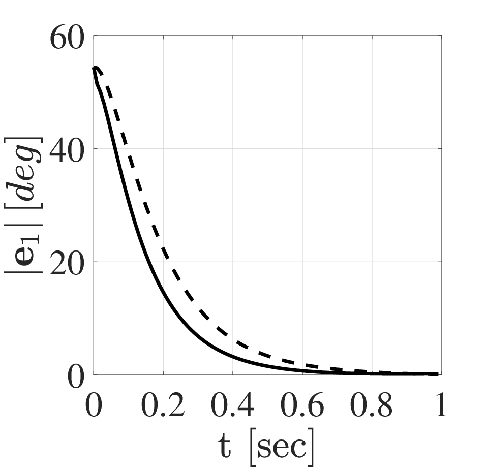
For comparing the trajectory tracking and the limit cycle tracking of the desired trajectory, the seven-link biped walking is simulated for the integrated CPG in the AS and AOS modes (i.e. and ). The results for the transition motion from standing to walking with the step length of and step period of are shown in Fig.16. The CPG parameters are selected such that the control effort for converging to the desired walking trajectory is the same for both modes. The results reveal that for , the robot converges to the desired walking trajectory faster than the case where . Thus, the limit cycle tracking of the desired trajectory provides a higher convergence rate with the same control effort in comparison with the trajectory tracking of the desired trajectory.



IX Conclusion
This paper presents a programmable oscillator that tracks multidimensional periodic trajectories. The programmable oscillator ensures the global stability and convergence of the desired trajectory and can also provide both asymptotic stability and asymptotic orbital stability of the desired trajectory according to an oscillator parameter. The programmable oscillator is also modified by a parametrization technique for bounding the output signal and its first time derivative. We used Lyapunov analysis to prove the global convergence to the desired trajectory for both original and modified oscillators. Both oscillators feature a parameter that controls the convergence to achieve either asymptotic stability (trajectory tracking) or asymptotic orbital stability (limit cycle tracking) of the desired trajectory. Finally, we presented an integrated CPG architecture based on the bounded output programmable oscillator. The proposed architecture is specifically designed for robotic applications where motion modulation is required. The proposed CPG generates smooth, synchronized, and bounded reference trajectory tracking the desired one from any initial condition irrespective of the parameters of the CPG. The desired trajectory is a multidimensional function whose components are either periodic functions or constants. This property is important for those applications where both periodic motions and constant posturing are required. Moreover, the proposed CPG can provide both trajectory tracking and limit cycle tracking of the desired trajectory. Accordingly, one can use the proposed CPG in the automatic or imitating modes. In the automatic mode, the oscillator guarantees the limit cycle tracking of the desired trajectory provided by a library. In the imitating mode, the CPG guarantees trajectory tracking of the desired trajectory measuring online from a human or another robot. The proposed CPG is a reliable and programmable architecture for online motion modulation. We validated the soundness of the proposed CPG with robotic rehabilitation experiments on the Kuka iiwa robot arm, and also walking simulations on a seven-link biped.
Appendix A Proof of Theorem 1
Theorem 1 has 3 items that we prove them in the following.
A-A is bounded and converges to from …
Starting with
| (22) |
where is the PD matrix used in (1b) and
the time derivative of along the system trajectory (1b) is
| (23) |
Since is a PD matrix and is a nonnegative constant, . Moreover, (22) shows that where iff . Hence and are bounded. Assuming that and its first time derivative are bounded, one also concludes the boundedness of for any initial condition. To get convergence of (or ), it is sufficient to examine the largest invariant subset of the set . Considering (1b), it is possible to verify that is the only invariant subset of . Therefore, according to the LaSalle Lemma [22], we can conclude that converges to . The global convergence of to is the consequence of the radially unbounded property of w.r.t. .
A-B if , then is globally AS
A-C if , then is the globally stable limit cycle
The limit cycle tracking and the trajectory tracking concepts are the same for a constant desired trajectory (see Section IV-A). The trajectory tracking of any desired trajectory including a constant one is proved in part A-B. In the following, we discuss the limit cycle tracking of a non-constant desired trajectory.
To investigate the stability of the set , we prove that for ,
- •
,
- •
, and
- •
,
where is the set of the states belonging to the trajectory of , i.e.
| (24) |
Thus, one can conclude that is the stable limit cycle of the system (1b) according to the extension of the Lyapunov stability theorem for invariant sets [23]. The global stability of the limit cycle is the result of the radially unbounded property of . For this purpose, we prove that for , iff . Therefore, the Lyapunov function presented in (22) satisfies the above three conditions, and we can conclude that is the globally stable limit cycle of the system. Since and , one can figure out that if , then . To prove that for , we have , we show that for and where is the -neighborhood of , is the point from the curve of in the shape space having the minimum distance from the current shape states. In this regard, we define the distance between and the curve of in the shape space as
| (25) |
where is the period of , and
| (26) | ||||
In the following, we prove that if . Since is continuous, its extreme is at . Thus, we consider the first and second derivatives of w.r.t. the phase state, i.e.
| (27) | ||||
The lower bound of is as
| (28) | ||||
On the other hand, considering (26), we have
| (29) | ||||
Considering the above relations, (28) is simplified as
| (30) | |||
where and . Note that is PD, and for a non-constant desired trajectory, that . Thus, one can find such that where is the -neighborhood of , we have . As a result, , iff . To investigate the time evolution of , we compute its time derivative along the trajectories of (1b) as
| (31) | ||||
Considering , the time derivative of is as
| (32) | ||||
where . Since , and , we have . Thus, we have
| (33) | ||||
Hence, for every if
| (34) |
we have
| (35) | ||||
Therefore, decreases when the trajectory enters . On the other hand, we have
| (36) |
where is the time instance that the trajectory of the system enters , and is the time instance when . From the above equation, one can concludes that . Hence, if , for all , we have , and thus .
Appendix B Proof of Theorem 2
Appendix C Proof of Theorem 3
Theorem 3 has 4 items which are proven in the following.
C-A is bounded and converges to from …
As the trajectory satisfies the differential equations (8d), is the response of the bounded output programmable oscillator for the initial condition . To prove the bounded property of , we consider
| (40) |
where , and
| (41) |
As , , and are diagonal positive definite matrices, is a PSD based on the Schur complement for block matrices [24]. Note that iff .
The time derivative of along the trajectories of the bounded output programmable oscillator is as
| (42) | ||||
where
| (43) | |||
As , and are diagonal PD matrices, and is a non-negative constant, . Thus, and are bounded. Moreover, as is radially unbounded w.r.t. , one can conclude that and are bounded from any initial condition. In conclusion, if , then the shape state vector is bounded for any initial condition.
For the convergence of to , it is sufficient to examine the largest invariant subset of . According to the dynamic (8d), is the only invariant subset of . Therefore, according to the LaSalle Lemma [22], we can conclude the convergence of to . The global convergence of is the result of the radially unbounded property of w.r.t. .
C-B if , is globally AS
C-C if , is the globally stable limit cycle
is the globally stable limit cycle iff is globally AS where is the set of the states belonging to , i.e. [22]
| (44) |
To investigate the AS of the set , we prove that for ,
- •
,
- •
, and
- •
.
Thus, is the stable limit cycle of the system (8d) according to the extension of the Lyapunov stability theorem for invariant sets [23]. The global stability of is the result of the radially unbounded property of . For this purpose, we prove that for , iff . Since and , one can figure out that if , then . To prove that for , we have , we show that for and where is the -neighborhood of , is the point from the curve of in the shape space having the minimum distance from the current shape states. In this regard, we define the distance between and the curve of in the shape space as
| (45) |
where is the period of and is as
| (46) | ||||
In the following, we prove that if . Since is continuous, its extreme is at . Thus, we consider the first and second derivatives of w.r.t. the phase state, i.e.
| (47) | ||||
The lower bound of is as
| (48) |
where is the minimum eigenvalue of , and . Note that is PD, thus . Since is positive and that , one can find such that where is the -neighborhood of , we have . As a result, , iff . To investigate time evolution of , we compute its time derivative along the trajectories of (8d) as
| (49) | ||||
Considering , the time derivative of is as
| (50) | ||||
where
| (51) |
and and . Based on (50), for if
| (52) |
then we have
| (53) |
Therefore, decreases when the trajectory enters . On the other hand, we have
| (54) |
where is the time instance that the trajectory of the system enters , is the time instance when , and . From the above equation, one can conclude that . Hence, if , for all , we have , and thus .
C-D the output converges to the curve of in …
As converges to , converges to the curve of in the shape . Moreover, according to the definition of in (8d) and the fact that is bounded, we have . In addition, based on the dynamic of the bounded output programmable oscillator, the time derivative of the output is as
| (55) |
Thus, . In conclusion, we have .
References
- [1] M. Mohanan and A. Salgoankar, “A survey of robotic motion planning in dynamic environments,” Robotics and Autonomous Systems, vol. 100, pp. 171–185, 2018.
- [2] R. Zhao, “Trajectory planning and control for robot manipulations,” Ph.D. dissertation, Université Paul Sabatier-Toulouse III, 2015.
- [3] J. Yu, M. Tan, J. Chen, and J. Zhang, “A survey on cpg-inspired control models and system implementation,” IEEE transactions on neural networks and learning systems, vol. 25, no. 3, pp. 441–456, 2014.
- [4] A. J. Ijspeert, J. Nakanishi, H. Hoffmann, P. Pastor, and S. Schaal, “Dynamical movement primitives: Learning attractor models for motor behaviors,” Neural Computation, vol. 25, no. 2, pp. 328–373, 2013.
- [5] M. Ajallooeian, J. van den Kieboom, A. Mukovskiy, M. A. Giese, and A. J. Ijspeert, “A general family of morphed nonlinear phase oscillators with arbitrary limit cycle shape,” Physica D: Nonlinear Phenomena, vol. 263, pp. 41–56, 2013.
- [6] M. Okada, K. Tatani, and Y. Nakamura, “Polynomial design of the nonlinear dynamics for the brain-like information processing of whole body motion,” in Proceedings 2002 IEEE International Conference on Robotics and Automation (Cat. No.02CH37292), vol. 2. IEEE, 2002, pp. 1410–1415.
- [7] M. Ajallooeian, M. N. Ahmadabadi, B. N. Araabi, and H. Moradi, “Design, implementation and analysis of an alternation-based central pattern generator for multidimensional trajectory generation,” Robotics and Autonomous Systems, vol. 60, no. 2, pp. 182–198, 2012.
- [8] V. Pasandi, A. Dinale, M. Keshmiri, and D. Pucci, “A programmable central pattern generator with bounded output,” Robotics and Autonomous Systems, vol. 125, p. 103423, 2020.
- [9] M. Faroni, R. Pagani, and G. Legnani, “Real-time trajectory scaling for robot manipulators,” in 2020 17th International Conference on Ubiquitous Robots (UR). IEEE, 2020, pp. 533–539.
- [10] E. Almasri and M. K. Uyguroğlu, “Trajectory optimization in robotic applications, survey of recent developments,” 2021.
- [11] R. Kaushik, T. Anne, and J.-B. Mouret, “Fast online adaptation in robotics through meta-learning embeddings of simulated priors,” in 2020 IEEE/RSJ International Conference on Intelligent Robots and Systems (IROS). IEEE, 2020, pp. 5269–5276.
- [12] C. H. Kim, H. Tsujino, and S. Sugano, “Online motion selection for semi-optimal stabilization using reverse-time tree,” in 2011 IEEE/RSJ International Conference on Intelligent Robots and Systems. IEEE, 2011, pp. 3792–3799.
- [13] D. G. Hobbelen and M. Wisse, “Limit cycle walking,” in Humanoid Robots, Human-like Machines. IntechOpen, 2007.
- [14] J. K. Hale, “Functional differential equations,” in Analytic theory of differential equations. Springer, 1971, pp. 9–22.
- [15] K. Hirai and K. Maeda, “A method of limit-cycle synthesis and its applications,” IEEE Transactions on Circuit Theory, vol. 19, no. 6, pp. 631–633, 1972.
- [16] D. Green, “Synthesis of systems with periodic solutions satisfying upsilon (x)= 0,” IEEE transactions on circuits and systems, vol. 31, no. 4, pp. 317–326, 1984.
- [17] K. Hirai and H. Chinen, “A synthesis of a nonlinear discrete-time system having a periodic solution,” IEEE Transactions on Circuits and Systems, vol. 29, no. 8, pp. 574–577, 1982.
- [18] V. Pasandi, A. Dinale, M. Keshmiri, and D. Pucci, “A data driven vector field oscillator with arbitrary limit cycle shape,” in 2019 IEEE 58th Conference on Decision and Control (CDC), 2019, pp. 8007–8012.
- [19] M. Charbonneau, F. Nori, and D. Pucci, “On-line joint limit avoidance for torque controlled robots by joint space parametrization,” in 2016 IEEE-RAS 16th International Conference on Humanoid Robots (Humanoids). IEEE, 2016, pp. 899–904.
- [20] Y. Farzaneh, A. Akbarzadeh, and A. A. Akbari, “Online bio-inspired trajectory generation of seven-link biped robot based on t–s fuzzy system,” Applied Soft Computing, vol. 14, pp. 167–180, 2014.
- [21] M. Vukobratović and B. Borovac, “Zero-moment point—thirty five years of its life,” International journal of humanoid robotics, vol. 1, no. 01, pp. 157–173, 2004.
- [22] H. K. Khalil and J. W. Grizzle, Nonlinear systems. Prentice hall Upper Saddle River, NJ, 2002, vol. 3.
- [23] V. I. Zubov, Methods of AM Lyapunov and their Application. P. Noordhoff, 1964.
- [24] F. Zhang, The Schur complement and its applications. Springer Science & Business Media, 2006, vol. 4.
![[Uncaptioned image]](2204.07766v1/authorPhoto/venusPasandi.JPG) |
Venus Pasandi received her bachelor and master degrees in mechanical engineering from Isfahan University of Technology, Iran and Amirkabir University of Technology, Iran in 2010 and 2012, respectively. In 2020, she earned her PhD title in Mechanical Engineering (Robotics and Control) from Isfahan University of Technology, Iran. From 2018-2019, she was a PhD student fellow in the Dynamic Interaction Control lab at Istituto Italiano di Tecnologia, Italy. She is currently a post-doctoral researcher in the Artificial and Mechanical Intelligence lab at Istituto Italiano di Tecnologia, Italy. Her current research interests include nonlinear systems and control, robotics, trajectory planning, and optimization. |
![[Uncaptioned image]](2204.07766v1/hamidSadeghian.png) |
Hamid Sadeghian received the B.Sc. and M.Sc. degrees in Mechanical Engineering from Isfahan University of Technology and Sharif University of Technology, Tehran, Iran, in 2005 and 2008, respectively. He received the Ph.D. degree in mechanical engineering (robotics and control) from Isfahan University of Technology in 2013. From November 2010 to January 2013, he was a visiting scholar with PRISMA Laboratory, Department of Electrical Engineering and Information Technology, University of Naples, Naples, Italy. Starting from 2013 he is an assistant professor of Control and Robotics with Engineering Dept. in University of Isfahan. In Sep. 2015 he visited Institute of Cognitive System at Technical University of Munich and German Aerospace Center (DLR), Munich, Germany, for one year post-doctoral research on locomotion of bipeds. His research interests include physical human-robot interaction/cooperation, medical robotics, and nonlinear control of mechanical systems. He is currently a senior scientist at Munich Institute of Robotics and Machine Intelligence, Technical University of Munich, Munich, Germany. |
![[Uncaptioned image]](2204.07766v1/authorPhoto/mehdiKeshmiri.jpg) |
Mehdi Keshmiri received his BSc and MSc degrees in Mechanical Engineering from Sharif University of Technology, Iran, in 1986 and 1989, respectively. He holds a PhD in Mechanical Engineering (space dynamics) from McGill University, Montreal, Canada. He is currently a Full Professor in the Department of Mechanical Engineering of Isfahan University of Technology (IUT), Isfahan, Iran. His research is mainly focused on system dynamics, control systems and dynamics and control of robotic systems. He has presented and published more than 150 papers in international conferences and journals and supervised more than 80 PhD and master students. He has been also involved in science and technology park development in Iran and is known as one of the leaders in this regard. |
![[Uncaptioned image]](2204.07766v1/authorPhoto/danielePucci.jpg) |
Daniele Pucci received the bachelor and master degrees in Control Engineering with highest honors from ”Sapienza”, University of Rome, in 2007 and 2009, respectively. In 2009, he also received the ”Excellence Path Award” from Sapienza. In 2013, he earned the PhD title with a thesis prepared at INRIA Sophia Antipolis, France, under the supervi- sion of Tarek Hamel and Claude Samson. The PhD program was jointly with ”Sapienza”, University of Rome, so in 2013 Daniele received also the PhD title in Control Engineering from Sapienza with the supervision of Salvatore Monaco. From 2013 to 2017, he has been a postdoc at the Istituto Italiano di Tecnologia (IIT) working within the EU project CoDyCo. From August 2017 to August 2021, he has been the head of the Dynamic Interaction Control lab. The main lab research focus was on the humanoid robot locomotion and physical interaction problem, with specific attention on the control and planning of the associated nonlinear systems. Also, the lab has been pioneering Aerial Humanoid Robotics, whose main aim is to make flying humanoid robots. Daniele has also been the scientific PI of the H2020 European Project AnDy, he is task leader of the H2020 European Project SoftManBot, and he is the coordinator of the joint laboratory between IIT and Honda JP. In 2019, he was awarded as Innovator of the year Under 35 Europe from the MIT Technology Review magazine. Since 2020 and in the context of the split site PhD supervision program, Daniele is a visiting lecturer at University of Manchester. In July 2020, Daniele was selected as a member of the Global Partnership on Artificial Intelligence (GPAI). Since September 1st 2021, Daniele is the PI leading the Artificial and Mechanical Intelligence research line at IIT. The research team combines AI and Mechanics to devise the next generation of Humanoid Robots. |