Safe Self-Refinement for Transformer-based Domain Adaptation
Abstract
Unsupervised Domain Adaptation (UDA) aims to leverage a label-rich source domain to solve tasks on a related unlabeled target domain. It is a challenging problem especially when a large domain gap lies between the source and target domains. In this paper we propose a novel solution named SSRT (Safe Self-Refinement for Transformer-based domain adaptation), which brings improvement from two aspects. First, encouraged by the success of vision transformers in various vision tasks, we arm SSRT with a transformer backbone. We find that the combination of vision transformer with simple adversarial adaptation surpasses best reported Convolutional Neural Network (CNN)-based results on the challenging DomainNet benchmark, showing its strong transferable feature representation. Second, to reduce the risk of model collapse and improve the effectiveness of knowledge transfer between domains with large gaps, we propose a Safe Self-Refinement strategy. Specifically, SSRT utilizes predictions of perturbed target domain data to refine the model. Since the model capacity of vision transformer is large and predictions in such challenging tasks can be noisy, a safe training mechanism is designed to adaptively adjust learning configuration. Extensive evaluations are conducted on several widely tested UDA benchmarks and SSRT achieves consistently the best performances, including 85.43% on Office-Home, 88.76% on VisDA-2017 and 45.2% on DomainNet.
1 Introduction
Deep neural networks have achieved impressive performance in a variety of machine learning tasks. However, the success often relies on a large amount of labeled training data, which can be costly or impractical to obtain. Unsupervised Domain Adaptation (UDA) wilson2020survey handles this issue by transferring knowledge from a label-rich source domain to a different unlabeled target domain. Over the past years, many UDA methods have been proposed ganin2015unsupervised; long2018conditional; zhang2019bridging; shu2018dirt; liang2020we. Among them, adversarial adaptation ganin2015unsupervised; long2018conditional; zhang2019bridging that learns domain-invariant feature representation using the idea of adversarial learning has been a prevailing paradigm. Deep UDA methods are usually applied in conjunction with a pretrained Convolutional Neural Network (CNN, e.g., ResNet he2016deep) backbone in vision tasks. On medium-sized classification benchmarks such as Office-Home venkateswara2017deep and VisDA peng2017visda, the reported state-of-the-arts are very impressive liang2020we. However, on large-scale datasets like DomainNet peng2019moment, the most recent results in the literature by our submission report a best average accuracy of 33.3% li2021semantic, which is far from satisfactory.
With the above observations, we focus our investigation on challenging cases from two aspects:
-
First, from the representation aspect, it is desirable to use a more powerful backbone network. This directs our attention to the recently popularized vision transformers, which have been successfully applied to various vision tasks dosovitskiy2020image; carion2020end; zhang2021multi. Vision transformer processes an image as a sequence of tokens, and uses global self-attention to refine this representation. With its long-range dependencies and large-scale pre-training, vision transformer obtains strong feature representation that is ready for down-stream tasks. Despite this, its application in UDA is still under-explored. Hence we propose to integrate vision transformer to UDA. We find that by simply combining ViT-B/16 dosovitskiy2020image with adversarial adaptation, it can achieve 38.5% average accuracy on DomainNet, better than the current arts using ResNet-101he2016deep; li2021semantic. This shows that the feature representation of vision transformer is discriminative as well as transferable across domains.
-
Second, from the domain adaptation aspect, a more reliable strategy is needed to protect the learning process from collapse due to large domain gaps. As strong backbones with large capacity like vision transformer increase the chance of overfitting to source domain data, a regularization from target domain data is desired. A common practice in UDA is to utilize model predictions for self-training or enforce clustering structure on target domain data zhang2020label; shu2018dirt; liang2020we. While this helps generally, the supervisions can be noisy when the domain gap is large. Therefore, an adaptation method is expected to be Safe li2014towards enough to avoid model collapse.
Motivated by the above discussions, in this paper, we propose a novel UDA solution named SSRT (Safe Self-Refinement for Transformer-based domain adaptation). SSRT takes a vision transformer as the backbone network and utilizes predictions on perturbed target domain data to refine the adapted model. Specifically, we add random offsets to the latent token sequences of target domain data, and minimize the discrepancy of model’s predicted probabilities between the original and perturbed versions using the Kullback Leibler (KL) divergence. This imposes a regularization on the corresponding transformer layers in effect. Moreover, SSRT has several important components that contribute to its excellent performance, including multi-layer perturbation and bi-directional supervision.
To protect the learning process from collapse, we propose a novel Safe Training mechanism. As UDA tasks vary widely even when they are drawn from the same dataset, a specific learning configuration (e.g., hyper-parameters) that works on most tasks may fail on some particular ones. The learning configuration is thus desired to be automatically adjustable. For example, for perturbation-based methods miyato2018virtual; sohn2020fixmatch, a small perturbation may under-exploit their benefits while a large one may result in collapse. Recent works tarvainen2017mean; berthelot2019mixmatch apply a manually defined ramp-up period at the beginning of training. However, this cannot solve the issue when its maximum value is improper for the current task. In contrast, we propose to monitor the whole training process and adjust learning configuration adaptively. We use a diversity measure of model predictions on the target domain data to detect model collapse. Once it occurs, the model is restored to a previously achieved state and the configuration is reset. With this safe training strategy, our SSRT avoids significant performance deterioration on adaptation tasks with large domain gaps. The code is available at https://github.com/tsun/SSRT.
In summary, we make the following contributions:
-
We develop a novel UDA solution SSRT, which adopts a vision transformer backbone for its strong transferable feature representation, and utilizes the predictions on perturbed target domain data for model refinement.
-
We propose a safe training strategy to protect the learning process from collapse due to large domain gaps. It adaptively adjusts learning configuration during the training process with a diversity measure of model predictions on target domain data.
-
SSRT is among the first to explore vision transformer for domain adaptation. Vision transformer-based UDA has shown promising results, especially on large-scale datasets like DomainNet.
-
Extensive experiments are conducted on widely tested benchmarks. Our SSRT achieves the best performances, including 85.43% on Office-Home, 88.76% on VisDA-2017 and 45.2% on DomainNet.

2 Related Work
Unsupervised Domain Adaptation.
There are several prevailing categories of UDA methods. Discrepancy-based methods minimize the distribution divergence between source and target domains with discrepancy measures tzeng2014deep; long2017deep; sun2016deep. Adversarial adaptation methods learn domain-invariant representations by playing a two-player min-max game between the feature extractor and a domain discriminator tzeng2014deep; sun2016deep; ganin2015unsupervised; tzeng2017adversarial. Recently, many works exploit self-training for domain adaptation mei2020instance; zou2019confidence; zou2018unsupervised. They generate pseudo labels for target domain data and take them as labeled data to refine the model.
Transformer in Vision.
Vision Transformer (ViT) dosovitskiy2020image is a pioneering work that applies a convolution-free transformer structure for image classification. Following that, many ViT variants have been proposed touvron2021training; yin2020disentangled; han2021transformer; liu2021swin. Transformer has been applied successfully to various vision tasks including image classification dosovitskiy2020image; touvron2021training, object detection carion2020end, semantic segmentation strudel2021segmenter, etc.
The application of vision transformer in domain adaptation, however, is still very scarce. Notably, two concurrent explorations xu2021cdtrans; yang2021tvt have been recently reported on arXiv. Specifically, CDTrans xu2021cdtrans is a pure transformer solution for UDA, and it applies cross attention on source-target image pairs. TVT yang2021tvt proposes a transferable multi-head self-attention module and combines it with adversarial adaptation. Our method is different in that it uses pairs of target domain data and their perturbed version to refine the model. This guarantees the same semantic class. Besides, we delicately design the components of our model and the training strategy to avoid collapse on challenging tasks.
Consistency Regularization.
Consistency regularization is an important technique in semi-supervised learning that achieves state-of-the-art results sohn2020fixmatch. It leverages the idea that model predictions should be similar for semantically identical data. Some methods create perturbed inputs with adversarial training miyato2018virtual, while others use standard data augmentations berthelot2019mixmatch; sohn2020fixmatch; xie2019unsupervised. These works mostly manipulate raw input images. In contrast, our study focuses on the latent token sequence representation of vision transformer.
3 Proposed Method
3.1 Problem Formulation
In Unsupervised Domain Adaptation, there is a source domain with labeled data from and a target domain with unlabeled data from , where is the input space and is the label space. UDA aims to learn a classifier , where denotes the feature extractor, denotes the class predictor, and is the latent space. Adversarial adaptation learns domain-invariant feature via a binary domain discrimination that maps features to domain labels.
The objective is formulated as
| (1) |
where is the standard cross-entropy loss on source domain data, is domain adversarial loss, defined as
is a trade-off parameter, and is a loss on target domain data. A common choice of is the Mutual Information Maximization loss gomes2010discriminative; shi2012information. In our method, we instantiate it as the self-refinement loss , introduced in Sec. 3.4.
3.2 Method Framework
We aim to regularize the latent feature spaces of transformer backbone by refining the model with perturbed target domain data. Figure 1 illustrates the framework of our proposed SSRT. Only target domain data are shown here. The network consists of a vision transformer backbone and a classifier head. Domain discriminator is not plotted. For each target domain image, the Patch Embedding layer transforms it into a token sequence including a special class token and image tokens. Then the sequence is refined with a series of Transformer Blocks. The classifier head takes the class token and outputs label prediction. We randomly choose one transformer block and add a random offset to its input token sequence. Then the corresponding predicted class probabilities of original and perturbed versions are used for bi-directional self-refinement. To avoid noisy supervision, only reliable predictions are used via a Confidence Filter. To reduce the risk of model collapse, we use a safe training mechanism to learn the model.
3.3 Multi-layer Perturbation for Transformer
While many works manipulate the raw input images miyato2018virtual; berthelot2019mixmatch; sohn2020fixmatch, it may be better to do that at hidden layers verma2019manifold. Vision transformer has some particular properties due to its special architecture. Since the Patch Embedding layer is merely a convolutional layer plus the position embedding, a linear operation on raw input can be shifted equivalently to the first transformer block. Besides, due to residual connections within transformer blocks, the token sequences at adjacent blocks are highly correlated. The best layer to add perturbation, however, varies across tasks. Empirically, perturbing relatively deep layers performs better but at a higher risk of model collapse. Therefore, we randomly choose one from multiple layers, which proves to be more robust than perturbing any single layer from them. In fact, it imposes a regularization on multiple layers simultaneously, making the learning process safer.
Given a target domain image , let be its input token sequence of the -th transformer block. can be viewed as a latent representation of in a hidden space. Since its dimension is high while the support of target domain data is limited in the space, it is inefficient to perturb arbitrarily. Instead, we utilize the token sequence of another randomly chosen target domain image to add an offset. The perturbed token sequence of is obtained as
| (2) |
where is a scalar and means no gradient back-propagation. Note that although gradients cannot back-propagate through the offset, they can pass through . The importance of this is elaborated in the following section.
In addition to the manually injected perturbation, the Dropout layer in the classifier head also works randomly for the two branches. This creates another source of discrepancy for the self-refinement loss.
3.4 Bi-directional Self-Refinement
Now we are ready to define the loss function used for self-refinement. Let and be the predicted probability vectors corresponding to and , respectively. To measure their distance, KL divergence is commonly used.
| (3) |
where is the teacher probability (a.k.a. target probability) and is the student probability. Note that KL divergence is asymmetric in and . While it is natural to take as the teacher probability since it corresponds to the original data, we find the reverse also works. Moreover, as shown in Sec. 4.3, it is more robust to combine them together. Our bi-directional self-refinement loss is defined as
| (4) | ||||
where is a random variable drawn from a Bernoulli distribution , is a Confidence Filter defined as
| (5) |
and is a predefined threshold. refines the model with confident predictions and regularizes it to predict smoothly in the latent feature spaces.
Typically, the loss gradient is only back-propagated through the student probability (i.e., in Eq. 3) miyato2018virtual; oliver2018realistic; berthelot2019mixmatch. We find, however, it is better to back-propagate gradient through both teacher and student probabilities in our framework. Recall that is propagated to identically in Eq. 2. Each model parameter is therefore updated based on the joint effects from and . This avoids excessively large gradients from any single probability. We observe degraded performance when either the gradients of teacher probabilities in KL divergence or that of are blocked.
3.5 Safe Training via Adaptive Adjustment
In the proposed self-refinement strategy, setting a proper value of the perturbation scalar and the self-refinement loss weight is critical. Excessively large perturbations lead to a collapse of the predicted class distribution, while a small one may under-exploit its benefit. Since the target domain is fully unlabeled and domain adaptation tasks vary widely even for the same dataset, it is desired to adjust these values adaptively. Some works tarvainen2017mean; berthelot2019mixmatch apply a ramp-up period at the beginning of training. While this alleviates the tendency to collapse during this period, it cannot solve the issue when the maximum value is improper for current adaptation tasks.
| Method | ArCl | ArPr | ArRw | ClAr | ClPr | ClRw | PrAr | PrCl | PrRw | RwAr | RwCl | RwPr | Avg. |
| ResNet-50 he2016deep | 34.9 | 50.0 | 58.0 | 37.4 | 41.9 | 46.2 | 38.5 | 31.2 | 60.4 | 53.9 | 41.2 | 59.9 | 46.1 |
| CDAN+E long2018conditional | 50.7 | 70.6 | 76.0 | 57.6 | 70.0 | 70.0 | 57.4 | 50.9 | 77.3 | 70.9 | 56.7 | 81.6 | 65.8 |
| SAFN xu2019larger | 52.0 | 71.7 | 76.3 | 64.2 | 69.9 | 71.9 | 63.7 | 51.4 | 77.1 | 70.9 | 57.1 | 81.5 | 67.3 |
| CDAN+TN wang2019transferable | 50.2 | 71.4 | 77.4 | 59.3 | 72.7 | 73.1 | 61.0 | 53.1 | 79.5 | 71.9 | 59.0 | 82.9 | 67.6 |
| SHOT liang2020we | 57.1 | 78.1 | 81.5 | 68.0 | 78.2 | 78.1 | 67.4 | 54.9 | 82.2 | 73.3 | 58.8 | 84.3 | 71.8 |
| DCAN+SCDA li2021semantic | 60.7 | 76.4 | 82.8 | 69.8 | 77.5 | 78.4 | 68.9 | 59.0 | 82.7 | 74.9 | 61.8 | 84.5 | 73.1 |
| CDTrans∗xu2021cdtrans | 68.8 | 85.0 | 86.9 | 81.5 | 87.1 | 87.3 | 79.6 | 63.3 | 88.2 | 82.0 | 66.0 | 90.6 | 80.5 |
| TVT∘ yang2021tvt | 74.89 | 86.82 | 89.47 | 82.78 | 87.95 | 88.27 | 79.81 | 71.94 | 90.13 | 85.46 | 74.62 | 90.56 | 83.56 |
| ViT-S dosovitskiy2020image | 47.01 | 76.98 | 83.54 | 69.84 | 77.11 | 80.42 | 68.15 | 44.08 | 82.86 | 74.78 | 47.97 | 84.66 | 69.78 |
| Baseline-S | 59.59 | 80.11 | 84.67 | 73.84 | 78.49 | 81.36 | 74.41 | 59.82 | 86.27 | 80.10 | 62.59 | 87.23 | 75.71 |
| SSRT-S (ours) | 67.03 | 84.21 | 88.32 | 79.85 | 84.28 | 87.58 | 80.72 | 66.03 | 88.27 | 82.04 | 69.44 | 89.86 | 80.64 |
| ViT-B dosovitskiy2020image | 54.68 | 83.04 | 87.15 | 77.30 | 83.42 | 85.54 | 74.41 | 50.90 | 87.22 | 79.56 | 53.79 | 88.80 | 75.48 |
| Baseline-B | 66.96 | 85.74 | 88.07 | 80.06 | 84.12 | 86.67 | 79.52 | 67.03 | 89.44 | 83.64 | 70.15 | 91.17 | 81.05 |
| Baseline-B+MI | 70.63 | 88.62 | 89.99 | 82.08 | 87.84 | 89.28 | 81.01 | 68.82 | 91.26 | 85.17 | 71.66 | 92.45 | 83.23 |
| SSRT-B (ours) | 75.17 | 88.98 | 91.09 | 85.13 | 88.29 | 89.95 | 85.04 | 74.23 | 91.26 | 85.70 | 78.58 | 91.78 | 85.43 |
|
clp | inf | pnt | qdr | rel | skt | Avg. |
|
clp | inf | pnt | qdr | rel | skt | Avg. | CDAN long2018conditional | clp | inf | pnt | qdr | rel | skt | Avg. | ||||
| clp | - | 19.3 | 37.5 | 11.1 | 52.2 | 41.0 | 32.2 | clp | - | 15.1 | 35.6 | 10.7 | 51.5 | 43.1 | 31.2 | clp | - | 20.4 | 36.6 | 9.0 | 50.7 | 42.3 | 31.8 | ||||
| inf | 30.2 | - | 31.2 | 3.6 | 44.0 | 27.9 | 27.4 | inf | 32.1 | - | 31.0 | 2.9 | 48.5 | 31.0 | 29.1 | inf | 27.5 | - | 25.7 | 1.8 | 34.7 | 20.1 | 22.0 | ||||
| pnt | 39.6 | 18.7 | - | 4.9 | 54.5 | 36.3 | 30.8 | pnt | 40.1 | 14.7 | - | 4.2 | 55.4 | 36.8 | 30.2 | pnt | 42.6 | 20.0 | - | 2.5 | 55.6 | 38.5 | 31.8 | ||||
| qdr | 7.0 | 0.9 | 1.4 | - | 4.1 | 8.3 | 4.3 | qdr | 18.8 | 3.1 | 5.0 | - | 16.0 | 13.8 | 11.3 | qdr | 21.0 | 4.5 | 8.1 | - | 14.3 | 15.7 | 12.7 | ||||
| rel | 48.4 | 22.2 | 49.4 | 6.4 | - | 38.8 | 33.0 | rel | 48.5 | 19.0 | 47.6 | 5.8 | - | 39.4 | 32.1 | rel | 51.9 | 23.3 | 50.4 | 5.4 | - | 41.4 | 34.5 | ||||
| skt | 46.9 | 15.4 | 37.0 | 10.9 | 47.0 | - | 31.4 | skt | 51.7 | 16.5 | 40.3 | 12.3 | 53.5 | - | 34.9 | skt | 50.8 | 20.3 | 43.0 | 2.9 | 50.8 | - | 33.6 | ||||
| Avg. | 34.4 | 15.3 | 31.3 | 7.4 | 40.4 | 30.5 | 26.6 | Avg. | 38.2 | 13.7 | 31.9 | 7.2 | 45.0 | 32.8 | 28.1 | Avg. | 38.8 | 17.7 | 32.8 | 4.3 | 41.2 | 31.6 | 27.7 | ||||
|
clp | inf | pnt | qdr | rel | skt | Avg. |
|
clp | inf | pnt | qdr | rel | skt | Avg. | ViT-B dosovitskiy2020image | clp | inf | pnt | qdr | rel | skt | Avg. | ||||
| clp | - | 20.4 | 43.3 | 15.2 | 59.3 | 46.5 | 36.9 | clp | - | 27.9 | 57.6 | 27.9 | 73.0 | 58.8 | 49.0 | clp | - | 27.2 | 53.1 | 13.2 | 71.2 | 53.3 | 43.6 | ||||
| inf | 32.7 | - | 34.5 | 6.3 | 47.6 | 29.2 | 30.1 | inf | 58.6 | - | 53.4 | 9.6 | 71.1 | 47.6 | 48.1 | inf | 51.4 | - | 49.3 | 4.0 | 66.3 | 41.1 | 42.4 | ||||
| pnt | 46.4 | 19.9 | - | 8.1 | 58.8 | 42.9 | 35.2 | pnt | 60.7 | 24.0 | - | 13.0 | 69.8 | 49.6 | 43.4 | pnt | 53.1 | 25.6 | - | 4.8 | 70.0 | 41.8 | 39.1 | ||||
| qdr | 31.1 | 6.6 | 18.0 | - | 28.8 | 22.0 | 21.3 | qdr | 2.9 | 0.4 | 0.3 | - | 0.7 | 4.7 | 1.8 | qdr | 30.5 | 4.5 | 16.0 | - | 27.0 | 19.3 | 19.5 | ||||
| rel | 55.5 | 23.7 | 52.9 | 9.5 | - | 45.2 | 37.4 | rel | 49.3 | 18.7 | 47.8 | 9.4 | - | 33.5 | 31.7 | rel | 58.4 | 29.0 | 60.0 | 6.0 | - | 45.8 | 39.9 | ||||
| skt | 55.8 | 20.1 | 46.5 | 15.0 | 56.7 | - | 38.8 | skt | 66.8 | 23.7 | 54.6 | 27.5 | 68.0 | - | 48.1 | skt | 63.9 | 23.8 | 52.3 | 14.4 | 67.4 | - | 44.4 | ||||
| Avg. | 44.3 | 18.1 | 39.0 | 10.8 | 50.2 | 37.2 | 33.3 | Avg. | 47.7 | 18.9 | 42.7 | 17.5 | 56.5 | 38.8 | 37.0 | Avg. | 51.5 | 22.0 | 46.1 | 8.5 | 60.4 | 40.3 | 38.1 | ||||
| Baseline-B | clp | inf | pnt | qdr | rel | skt | Avg. |
|
clp | inf | pnt | qdr | rel | skt | Avg. |
|
clp | inf | pnt | qdr | rel | skt | Avg. | ||||
| clp | - | 30.9 | 53.3 | 16.3 | 72.7 | 55.4 | 45.7 | clp | - | 30.5 | 55.8 | 18.1 | 74.7 | 57.5 | 47.3 | clp | - | 33.8 | 60.2 | 19.4 | 75.8 | 59.8 | 49.8 | ||||
| inf | 43.0 | - | 40.8 | 7.8 | 56.4 | 35.9 | 36.8 | inf | 53.2 | - | 52.8 | 9.2 | 68.3 | 45.3 | 45.8 | inf | 55.5 | - | 54.0 | 9.0 | 68.2 | 44.7 | 46.3 | ||||
| pnt | 55.7 | 28.6 | - | 7.4 | 70.5 | 48.3 | 42.1 | pnt | 56.8 | 27.6 | - | 7.3 | 70.8 | 49.3 | 42.4 | pnt | 61.7 | 28.5 | - | 8.4 | 71.4 | 55.2 | 45.0 | ||||
| qdr | 25.5 | 5.2 | 9.7 | - | 15.5 | 17.1 | 14.6 | qdr | 31.6 | 5.1 | 13.3 | - | 25.3 | 23.0 | 19.6 | qdr | 42.5 | 8.8 | 24.2 | - | 37.6 | 33.6 | 29.3 | ||||
| rel | 62.3 | 32.5 | 62.5 | 8.2 | - | 50.7 | 43.2 | rel | 65.7 | 32.4 | 63.9 | 6.9 | - | 51.7 | 44.1 | rel | 69.9 | 37.1 | 66.0 | 10.1 | - | 58.9 | 48.4 | ||||
| skt | 66.4 | 30.6 | 58.0 | 18.1 | 70.1 | - | 48.6 | skt | 68.9 | 30.6 | 61.0 | 19.3 | 72.9 | - | 50.5 | skt | 70.6 | 32.8 | 62.2 | 21.7 | 73.2 | - | 52.1 | ||||
| Avg. | 50.6 | 25.6 | 44.9 | 11.6 | 57.0 | 41.5 | 38.5 | Avg. | 55.2 | 25.2 | 49.4 | 12.2 | 62.4 | 45.3 | 41.6 | Avg. | 60.0 | 28.2 | 53.3 | 13.7 | 65.3 | 50.4 | 45.2 |
| Method | plane | bcycl | bus | car | horse | knife | mcycl | person | plant | sktbrd | train | truck | Avg. |
| ResNet-101 he2016deep | 55.1 | 53.3 | 61.9 | 59.1 | 80.6 | 17.9 | 79.7 | 31.2 | 81.0 | 26.5 | 73.5 | 8.5 | 52.4 |
| DANN ganin2015unsupervised | 81.9 | 77.7 | 82.8 | 44.3 | 81.2 | 29.5 | 65.1 | 28.6 | 51.9 | 54.6 | 82.8 | 7.8 | 57.4 |
| CDAN long2018conditional | 85.2 | 66.9 | 83.0 | 50.8 | 84.2 | 74.9 | 88.1 | 74.5 | 83.4 | 76.0 | 81.9 | 38.0 | 73.9 |
| SAFN xu2019larger | 93.6 | 61.3 | 84.1 | 70.6 | 94.1 | 79.0 | 91.8 | 79.6 | 89.9 | 55.6 | 89.0 | 24.4 | 76.1 |
| SWD lee2019sliced | 90.8 | 82.5 | 81.7 | 70.5 | 91.7 | 69.5 | 86.3 | 77.5 | 87.4 | 63.6 | 85.6 | 29.2 | 76.4 |
| SHOT liang2020we | 94.3 | 88.5 | 80.1 | 57.3 | 93.1 | 94.9 | 80.7 | 80.3 | 91.5 | 89.1 | 86.3 | 58.2 | 82.9 |
| CDTrans∗xu2021cdtrans | 97.1 | 90.5 | 82.4 | 77.5 | 96.6 | 96.1 | 93.6 | 88.6 | 97.9 | 86.9 | 90.3 | 62.8 | 88.4 |
| TVT∘ yang2021tvt | 92.92 | 85.58 | 77.51 | 60.48 | 93.60 | 98.17 | 89.35 | 76.40 | 93.56 | 92.02 | 91.69 | 55.73 | 83.92 |
| ViT-B dosovitskiy2020image | 99.09 | 60.66 | 70.55 | 82.66 | 96.50 | 73.06 | 97.14 | 19.73 | 64.48 | 94.74 | 97.21 | 15.36 | 72.60 |
| Baseline-B | 98.55 | 82.59 | 85.97 | 57.07 | 94.93 | 97.20 | 94.58 | 76.68 | 92.11 | 96.54 | 94.31 | 52.24 | 85.23 |
| Baseline-B+MI | 98.63 | 90.79 | 81.83 | 47.28 | 96.29 | 98.36 | 84.68 | 70.70 | 93.30 | 97.54 | 94.55 | 55.03 | 84.08 |
| SSRT-B (ours) | 98.93 | 87.60 | 89.10 | 84.77 | 98.34 | 98.70 | 96.27 | 81.08 | 94.86 | 97.90 | 94.50 | 43.13 | 88.76 |
We propose a Safe Training mechanism. The observation is that whenever the model begins to collapse, the diversity of model predictions will decrease simultaneously. Our goal is to detect such events while monitoring the training process. Once it occurs, the learning configuration is reset and meanwhile the model is restored to a previously achieved state. Specifically, an adaptive scalar is adopted to modulate and , i.e., and . We define a fixed period and divide the training process into consecutive intervals. A model snapshot is saved at the end of each interval. Then is defined as
| (6) |
where is the current training step. Initially, and . It hence takes steps for to ramp up to 1.0. At the end of each interval, the diversity of model predictions within this interval is checked to find abrupt dropping. If not existed, the formulation of remains unchanged. Otherwise, is reset to current training step , and the model is restored to last snapshot. To avoid oscillation between collapse and restoration, is doubled if the last restoration occurs within steps. Figure 1 illustrates the training process with adaptive adjustment. Two events of diversity dropping are identified (marked with pink areas), leading to two model restorations and reset of .
The remaining issue is which diversity measure to use and how to detect diversity dropping. We find that the number of unique model predicted labels on each target training batch works well. We hence define the following diversity measure:
| (7) |
To detect diversity dropping, we split the interval into sub-intervals and check whether the average diversity value drops across each sub-interval. We implement this at multi-scales to improve the sensitivity of detection. Every consecutive sub-intervals of steps are checked for a given integer . Details are listed in Alg. 1 and Alg. 2.
4 Experiments
We evaluate our method on four popular UDA benchmarks. Office-31 saenko2010adapting contains 4,652 images of 31 classes from three domains: Amazon (A), DSLR (D) and Webcam (W). Office-Home venkateswara2017deep consists of 15,500 images of 65 classes from four domains: Artistic (Ar), Clip Art (Cl), Product (Pr), and Real-world (Rw) images. VisDA-2017 peng2017visda is a Synthetic-to-Real dataset, with about 0.2 million images in 12 classes. DomainNet peng2019moment is the largest DA dataset containing about 0.6 million images of 345 classes in 6 domains: Clipart (clp), Infograph (inf), Painting (pnt), Quickdraw (qdr), Real (rel), Sketch (skt).
We use the ViT-base and ViT-small with 1616 patch size dosovitskiy2020image; steiner2021augreg, pre-trained on ImageNet ILSVRC15, as the vision transformer backbones. For all tasks, we use an identical set of hyper-parameters (, , , , ). Ablation studies on them are provided in Sec. 4.6. More details can be found in the supplementary material.
Our comparison methods include DANN ganin2015unsupervised, CDAN long2018conditional, CDAN+E long2018conditional, SAFN xu2019larger, SAFN+ENT xu2019larger, CDAN+TN wang2019transferable, SHOT liang2020we, DCAN+SCDA li2021semantic, MDD+SCDA li2021semantic, SWD lee2019sliced, MIMTFEL gao2020reducing, TVT yang2021tvt and CDTrans xu2021cdtrans. “Baseline” is ViT with adversarial adaptation (see Sec. 3.1). We also include its combination with Mutual Information (MI) loss gomes2010discriminative; shi2012information in comparison.
4.1 Results on Benchmarks
Tables 1-4 present evaluation results on four benchmarks. We use “-S/B” to indicate results using ViT-small/base backbones, respectively. For Office-Home and Offce-31, CNN-based methods use ResNet-50 as their backbones; whereas for DomainNet and VisDA they use ResNet-101. Generally, the transformer-based results are much better. This is attributed to its strong transferable feature representations. ViT-base is better than ViT-small, due to higher model complexity. Apparently, Baselines improve over source-only training. Integrating Mutual Information (MI) loss further improves. Compared with other methods, SSRT-B performs the best on Office-Home, DomainNet and VisDA. It improves 4.38% on Office-Home, 3.53% on VisDA-2017 and 6.7% on DomainNet over Baseline-B despite that Baseline-B is already very strong. In particular, on the challenging DomainNet dataset, SSRT-B achieves an impressive 45.2% average accuracy. It is worth mentioning that in DomainNet some domains have large gaps from the others, such as inf and qdr. Transferring among these domains and others is very difficult. It is thus desired to transfer safely and not deteriorate the performance significantly. Looking at tasks with qdr being target domain, SSRT-B obtains 29.3% average accuracy, while many other methods perform poorly. We illustrate the effects of some important components that contribute to our excellent performance in the following sections.
| Method | AW | DW | WD | AD | DA | WA | Avg. |
| ResNet-50 he2016deep | 68.4 | 96.7 | 99.3 | 68.9 | 62.5 | 60.7 | 76.1 |
| DANN ganin2015unsupervised | 82.0 | 96.9 | 99.1 | 79.7 | 68.2 | 67.4 | 82.2 |
| SAFN+ENT xu2019larger | 90.1 | 98.6 | 99.8 | 90.7 | 73.0 | 70.2 | 87.1 |
| CDAN+TN wang2019transferable | 95.7 | 98.7 | 100. | 94.0 | 73.4 | 74.2 | 89.3 |
| SHOT liang2020we | 90.1 | 98.4 | 99.9 | 94.0 | 74.7 | 74.3 | 88.6 |
| MDD+SCDA li2021semantic | 95.3 | 99.0 | 100. | 95.4 | 77.2 | 75.9 | 90.5 |
| CDTrans∗xu2021cdtrans | 96.7 | 99.0 | 100. | 97.0 | 81.1 | 81.9 | 92.6 |
| TVT∘yang2021tvt | 96.4 | 99.4 | 100. | 96.4 | 84.9 | 86.1 | 93.8 |
| ViT-S dosovitskiy2020image | 86.9 | 98.6 | 100. | 88.6 | 76.0 | 75.9 | 87.7 |
| Baseline-S | 91.9 | 99.1 | 100. | 89.2 | 78.4 | 77.9 | 89.4 |
| SSRT-S (ours) | 95.7 | 99.2 | 100. | 95.8 | 79.2 | 79.9 | 91.6 |
| ViT-B dosovitskiy2020image | 91.2 | 99.2 | 100. | 90.4 | 81.1 | 80.6 | 90.4 |
| Baseline-B | 92.5 | 99.2 | 100. | 93.6 | 80.7 | 80.7 | 91.1 |
| SSRT-B (ours) | 97.7 | 99.2 | 100. | 98.6 | 83.5 | 82.2 | 93.5 |
| OH | DN | clp† | inf† | pnt† | qdr† | rel† | skt† | |
| Baseline-B | 81.1 | 38.5 | 50.6 | 25.6 | 44.9 | 11.6 | 57.0 | 41.5 |
| SSRT-B (raw) | 85.0 | 44.2 | 58.6 | 26.7 | 51.7 | 13.7 | 63.9 | 50.8 |
| SSRT-B | 85.4 | 45.2 | 60.0 | 28.2 | 53.3 | 13.7 | 65.3 | 50.4 |
4.2 Effects of Multi-layer Perturbation
Table 5 verifies that applying perturbation to the latent token sequences performs better than to the raw input images on Office-Home (OH) and DomainNet (DN). Fig. 5(a) compares performances when adding the same amount of perturbation to each layer while not using safe training. As can be seen, the best layer to apply perturbation varies across tasks. Besides, a layer that works for one task may fail on others. In our experiments, we uniformly choose one layer from {0,4,8}. As a comparison, perturbing any single layer from it decreases the average accuracy on DomainNet by -1.0%, -1.5% and -1.5%, respectively.
| OH | DN | clp† | inf† | pnt† | qdr† | rel† | skt† | |
| Baseline-B | 81.1 | 38.9 | 50.7 | 25.5 | 46.1 | 11.9 | 57.4 | 42.0 |
| 85.5 | 41.1 | 57.3 | 22.0 | 52.2 | 1.8 | 63.4 | 49.9 | |
| 85.7 | 40.1 | 56.6 | 23.4 | 48.1 | 0.3 | 63.3 | 49.0 | |
| 85.4 | 41.8 | 57.0 | 26.6 | 53.0 | 1.8 | 63.2 | 49.5 | |
| 85.4 | 43.4 | 57.0 | 28.2 | 51.8 | 13.0 | 62.9 | 47.4 |
4.3 Effects of Bi-directional Self-Refinement
Our method adopts bi-directional supervision for self-refinement in Eq. 4. The main consideration is to improve method’s safeness. Figure 3 compares with uni-directional self-refinement by fixing to be 0 or 1. In the upper two figures, their performance drops for relatively large confidence threshold . In the lower two figures, model collapse occurs after training for some steps. In contrast, bi-directional self-refinement is more robust as it combines the two losses, thus reduces the negative effect of either one. Table 6 presents some quantitative results. On Office-Home, all losses perform similarly well. On DomainNet, bi-directional self-refinement works better. However, they all fail on challenging tasks when target domain is qdr. This is solved with Safe Training.
Another important issue is when to back-propagate gradients. Table 7 shows that the performance degrades when either the gradient for in Eq. 2 or the teacher probability of KL divergence in Eq. 4 are blocked. An interesting finding is that the bi-directional self-refinement appears to be more robust even when the gradients are blocked. We believe this is because the two losses are complementary.
| PrAr | PrCl | PrRw | ||||
| 4.70 | 2.66 | 16.39 | ||||
| 79.15 | 44.38 | 89.14 | ||||
| 84.10 | 71.32 | 90.75 | ||||
| 84.38 | 72.60 | 90.87 | ||||
| 85.74 | 74.98 | 91.16 |
4.4 Effects of Safe Training
As observed previously, the vanilla training strategy may fail on some tasks. The reason is that the predicted class distribution on target domain data collapses due to excessive perturbation or too large loss weight, even if they work well on other tasks. Safe Training adjusts their values adaptively to avoid such situation. Figure 2 presents detailed training histories on two representative tasks to show how it works. For qdrclp, the adaptive scalar quickly converges to 1.0 and the diversity stabilizes to a relatively high value. Training model with or without Safe Training performs similarly. For clpqdr, diversity drops after some steps, and resets to smaller values. A clear correlation between diversity and accuracy can be observed. For example, at step of 10k, the accuracy drops abruptly and diversity drops concurrently. Without Safe Training, model collapses after about 10k iterations. With Safe Training, the model trains normally and surpasses the baseline finally. It should be noted that model collapse mainly affects target domain data. For clpqdr without safe training, the final accuracy on source domain is 96.9% while that on target domain is only 0.3%.
4.5 Visualization of Perturbation
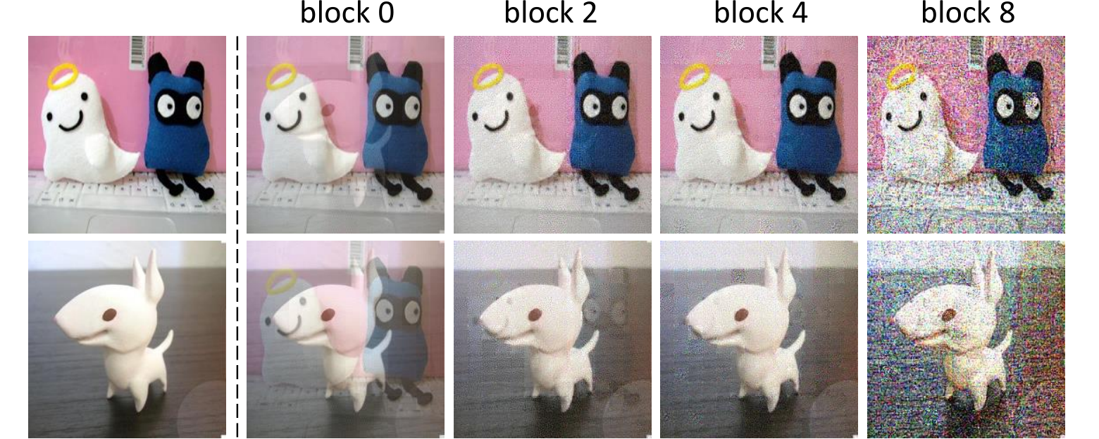
To visualize the perturbed version of a target domain image , we initialize a trainable variable as , and optimize to minimize , where is the perturbed token sequence of and is the corresponding token sequence of . Then gives us an idea on how the perturbation in the latent space reflects on the raw input images. Figure 4 visualizes perturbed version of two images when adding perturbation to different transformer blocks. For shallow layers, an effect of blending with the other image can be observed. However, for deep layers, this effect is less noticeable due to highly non-linear transformation of the network. This also indicates the complementary in using multi-layer perturbation.
4.6 Ablation Studies
Figure 5 presents ablation studies on hyper-parameters. Figure 5(a) plots results of perturbing different layers. Figure 5(b) plots Safe Training with different parameters. and affects its granularity. A smaller implies more quick response. A larger increases sensitivity but at the risk of more false-positive detections. Many combinations of and work well in our method. Figure 5(c) and 5(d) plots accuracy curves vs. the perturbation scalar and the self-refinement loss weight . Even for obviously unreasonable values like , Safe Training can still adjust them adaptively to avoid model collapse. When , our method still has some gain over baseline. This is due to random dropout operations in the classifier head.
5 Conclusion
In this paper, we propose a novel UDA method named SSRT. It leverages a vision transformer backbone, and uses perturbed target domain data to refine the model. A safe training strategy is developed to avoid model collapse. Experiments on benchmarks show its best performance.
Limitation. Although we advance the average accuracy on DomainNet to 45.2%, it is far from saturated. One way is to combine multiple source domains. Another way is to incorporate some meta knowledge about target domains. We plan to extend our study in these directions in the future.
Appendix A More Model and Training Details
Our implementation is based on the timm library11 1 https://github.com/rwightman/pytorch-image-models/blob/master/timm/models/vision_transformer.py. We use ViT-B/16 dosovitskiy2020image (vit_base_patch16_224 in timm) and ViT-S/16 dosovitskiy2020image (vit_small_patch16_224 in timm) as the vision transformer backbones in the paper. Transformer weights are restored from the checkpoints released by official Google JAX implementation22 2 https://github.com/google-research/vision_transformer, which are obtained by first training on ImageNet-21k ILSVRC15 and then fine-tuning on Image-1k steiner2021augreg; ILSVRC15. The classifier head consists of a bottleneck module (Linear BatchNorm1d ReLU Dropout(0.5)) and a class predictor (Linear ReLU Dropout(0.5) Linear). The domain discriminator has the same network structure as the class predictor except having only one output.
During the training procedure, images are first resized to pixels, randomly flipped horizontally, and then randomly cropped and resized to pixels. The only exception is for VisDA-2017 peng2017visda, where center-cropping of size is used. During the test procedure, images are first resized to pixels and then center-cropped to pixels. To train the model, we adopt mini-batch Stochastic Gradient Descent (SGD) with momentum of 0.9. Learning rate is scheduled as , where is initial learning rate, is training step. The learning rate of parameters of vision transformer backbone is set to be 1/10 of .
Appendix B More Analysis on Bi-directional Self-Refinement
Table A.1 provides additional results when blocking gradient back-propagation for different variables. Similar to the results listed in the paper (see Tab. 7), allowing gradient back-propagation of the teacher probabilities in KL divergence and works better than other variants.
Appendix C More Analysis on Safe Training
In our method, we adopt a Confidence Filter to remove noisy supervisions. If it not used (i.e., ), the performance may deteriorate. Table A.6 shows that using Safe Training can avoid significant performance drops, making the method much safer.
| ClAr | ClPr | ClRw | ||||
| 1.61 | 12.71 | 6.08 | ||||
| 81.17 | 85.00 | 87.28 | ||||
| 83.68 | 85.69 | 88.04 | ||||
| 84.55 | 87.27 | 89.49 | ||||
| 85.21 | 87.88 | 89.58 |
Appendix D More Analysis on Multi-layer Perturbation
Figure A.1 provides additional results when adding the same amount of perturbation to each layer while not using safe training. As can be seen in the left figure, the best layer to apply perturbation varies across tasks. Besides, a layer that works for one task may fail on others. To see the importance of allowing gradient back-propagation for (see Sec. 3.3 and Sec. 3.4 in the paper), the right figure shows that the model collapses when add perturbation to relatively deep layers while blocking the gradients of .
Table A.2 includes comparison results when adding the perturbation to raw input or a single layer ({0} or {4} or {8}) in our proposed SSRT method. As can be seen, perturbing raw input performs similarly to perturbing the 0-th transformer block. Besides, perturbing any single layer degrades the performance on some adaptations tasks. In contrast, multi-layer perturbation combines their merits and obtains the best results.
|
clp | inf | pnt | qdr | rel | skt | Avg. | ViT-B | clp | inf | pnt | qdr | rel | skt | Avg. | Baseline-B | clp | inf | pnt | qdr | rel | skt | Avg. | ||||||
| clp | - | 20.4 | 43.3 | 15.2 | 59.3 | 46.5 | 36.9 | clp | - | 27.2 | 53.1 | 13.2 | 71.2 | 53.3 | 43.6 | clp | - | 30.9 | 53.3 | 16.3 | 72.7 | 55.4 | 45.7 | ||||||
| inf | 32.7 | - | 34.5 | 6.3 | 47.6 | 29.2 | 30.1 | inf | 51.4 | - | 49.3 | 4.0 | 66.3 | 41.1 | 42.4 | inf | 43.0 | - | 40.8 | 7.8 | 56.4 | 35.9 | 36.8 | ||||||
| pnt | 46.4 | 19.9 | - | 8.1 | 58.8 | 42.9 | 35.2 | pnt | 53.1 | 25.6 | - | 4.8 | 70.0 | 41.8 | 39.1 | pnt | 55.7 | 28.6 | - | 7.4 | 70.5 | 48.3 | 42.1 | ||||||
| qdr | 31.1 | 6.6 | 18.0 | - | 28.8 | 22.0 | 21.3 | qdr | 30.5 | 4.5 | 16.0 | - | 27.0 | 19.3 | 19.5 | qdr | 25.5 | 5.2 | 9.7 | - | 15.5 | 17.1 | 14.6 | ||||||
| rel | 55.5 | 23.7 | 52.9 | 9.5 | - | 45.2 | 37.4 | rel | 58.4 | 29.0 | 60.0 | 6.0 | - | 45.8 | 39.9 | rel | 62.3 | 32.5 | 62.5 | 8.2 | - | 50.7 | 43.2 | ||||||
| skt | 55.8 | 20.1 | 46.5 | 15.0 | 56.7 | - | 38.8 | skt | 63.9 | 23.8 | 52.3 | 14.4 | 67.4 | - | 44.4 | skt | 66.4 | 30.6 | 58.0 | 18.1 | 70.1 | - | 48.6 | ||||||
| Avg. | 44.3 | 18.1 | 39.0 | 10.8 | 50.2 | 37.2 | 33.3 | Avg. | 51.5 | 22.0 | 46.1 | 8.5 | 60.4 | 40.3 | 38.1 | Avg. | 50.6 | 25.6 | 44.9 | 11.6 | 57.0 | 41.5 | 38.5 | ||||||
| VAT-Bmiyato2018virtual | clp | inf | pnt | qdr | rel | skt | Avg. |
|
clp | inf | pnt | qdr | rel | skt | Avg. |
|
clp | inf | pnt | qdr | rel | skt | Avg. | ||||||
| clp | - | 33.1 | 57.1 | 19.5 | 75.8 | 59.8 | 49.0 | clp | - | 32.7 | 60.0 | 19.0 | 75.3 | 59.8 | 49.3 | clp | - | 33.2 | 59.7 | 19.6 | 75.3 | 58.7 | 49.3 | ||||||
| inf | 48.3 | - | 45.2 | 9.8 | 55.0 | 37.4 | 39.2 | inf | 55.0 | - | 54.0 | 8.9 | 67.8 | 48.1 | 46.8 | inf | 54.8 | - | 53.5 | 9.3 | 67.7 | 46.1 | 46.3 | ||||||
| pnt | 60.0 | 30.9 | - | 7.9 | 71.1 | 52.6 | 44.5 | pnt | 61.6 | 28.6 | - | 8.2 | 71.3 | 55.4 | 45.0 | pnt | 61.2 | 29.0 | - | 7.1 | 71.2 | 55.0 | 44.7 | ||||||
| qdr | 26.7 | 5.4 | 9.2 | - | 18.1 | 18.3 | 15.5 | qdr | 36.3 | 6.2 | 16.1 | - | 32.1 | 31.2 | 24.4 | qdr | 40.8 | 7.0 | 13.2 | - | 35.4 | 31.1 | 25.5 | ||||||
| rel | 68.7 | 35.3 | 65.0 | 7.8 | - | 56.8 | 46.7 | rel | 69.8 | 35.6 | 66.1 | 12.4 | - | 59.2 | 48.6 | rel | 69.6 | 35.7 | 65.7 | 10.7 | - | 58.7 | 48.1 | ||||||
| skt | 70.2 | 33.3 | 65.0 | 17.6 | 72.2 | - | 51.7 | skt | 70.3 | 30.5 | 62.3 | 20.0 | 73.2 | - | 51.3 | skt | 69.7 | 32.1 | 62.0 | 19.0 | 72.8 | - | 51.1 | ||||||
| Avg. | 54.8 | 27.6 | 48.3 | 12.5 | 58.4 | 45.0 | 41.1 | Avg. | 58.6 | 26.7 | 51.7 | 13.7 | 63.9 | 50.8 | 44.2 | Avg. | 59.2 | 27.4 | 50.8 | 13.1 | 64.5 | 49.9 | 44.2 | ||||||
|
clp | inf | pnt | qdr | rel | skt | Avg. |
|
clp | inf | pnt | qdr | rel | skt | Avg. |
|
clp | inf | pnt | qdr | rel | skt | Avg. | ||||||
| clp | - | 31.8 | 58.9 | 17.8 | 75.7 | 59.4 | 48.7 | clp | - | 32.4 | 59.0 | 18.6 | 75.6 | 59.9 | 49.1 | clp | - | 33.8 | 60.2 | 19.4 | 75.8 | 59.8 | 49.8 | ||||||
| inf | 53.5 | - | 50.5 | 8.6 | 67.8 | 47.5 | 45.6 | inf | 55.9 | - | 54.8 | 7.6 | 68.5 | 48.2 | 47.0 | inf | 55.5 | - | 54.0 | 9.0 | 68.2 | 44.7 | 46.3 | ||||||
| pnt | 61.3 | 29.2 | - | 8.1 | 71.3 | 54.3 | 44.8 | pnt | 61.5 | 27.4 | - | 8.5 | 71.4 | 54.6 | 44.7 | pnt | 61.7 | 28.5 | - | 8.4 | 71.4 | 55.2 | 45.0 | ||||||
| qdr | 42.5 | 7.7 | 17.0 | - | 23.3 | 33.4 | 24.8 | qdr | 33.6 | 5.7 | 11.3 | - | 31.4 | 31.8 | 22.7 | qdr | 42.5 | 8.8 | 24.2 | - | 37.6 | 33.6 | 29.3 | ||||||
| rel | 68.7 | 36.1 | 65.5 | 8.2 | - | 57.6 | 47.2 | rel | 69.6 | 36.2 | 65.9 | 6.9 | - | 58.1 | 47.3 | rel | 69.9 | 37.1 | 66.0 | 10.1 | - | 58.9 | 48.4 | ||||||
| skt | 70.1 | 31.8 | 62.2 | 17.7 | 73.1 | - | 51.0 | skt | 69.9 | 30.9 | 62.3 | 19.8 | 73.3 | - | 51.2 | skt | 70.6 | 32.8 | 62.2 | 21.7 | 73.2 | - | 52.1 | ||||||
| Avg. | 59.2 | 27.3 | 50.8 | 12.1 | 62.2 | 50.4 | 43.7 | Avg. | 58.1 | 26.5 | 50.6 | 12.3 | 64.0 | 50.5 | 43.7 | Avg. | 60.0 | 28.2 | 53.3 | 13.7 | 65.3 | 50.4 | 45.2 | ||||||
| ViT-S | clp | inf | pnt | qdr | rel | skt | Avg. | Baseline-S | clp | inf | pnt | qdr | rel | skt | Avg. |
|
clp | inf | pnt | qdr | rel | skt | Avg. | ||||||
| clp | - | 23.0 | 46.2 | 11.9 | 66.3 | 46.2 | 38.7 | clp | - | 27.0 | 49.0 | 12.8 | 68.2 | 49.1 | 41.2 | clp | - | 28.5 | 53.1 | 12.1 | 69.9 | 52.1 | 43.1 | ||||||
| inf | 42.9 | - | 42.8 | 3.8 | 62.3 | 33.9 | 37.1 | inf | 41.8 | - | 43.1 | 2.7 | 63.0 | 33.0 | 36.7 | inf | 47.5 | - | 49.8 | 1.5 | 64.9 | 39.7 | 40.7 | ||||||
| pnt | 45.2 | 22.2 | - | 3.5 | 66.5 | 35.7 | 34.6 | pnt | 48.8 | 25.7 | - | 3.1 | 67.0 | 40.8 | 37.1 | pnt | 53.0 | 26.5 | - | 4.4 | 67.3 | 46.7 | 39.6 | ||||||
| qdr | 19.7 | 3.3 | 7.8 | - | 14.6 | 12.7 | 11.6 | qdr | 21.8 | 5.8 | 9.6 | - | 15.3 | 15.2 | 13.5 | qdr | 31.3 | 6.9 | 13.0 | - | 24.4 | 24.0 | 19.9 | ||||||
| rel | 50.8 | 24.2 | 54.2 | 4.6 | - | 37.3 | 34.2 | rel | 54.6 | 28.7 | 57.5 | 3.6 | - | 41.3 | 37.1 | rel | 60.0 | 31.2 | 60.5 | 4.6 | - | 48.5 | 41.0 | ||||||
| skt | 57.2 | 19.5 | 47.1 | 13.9 | 62.5 | - | 40.0 | skt | 60.9 | 26.2 | 53.9 | 10.6 | 67.5 | - | 43.8 | skt | 63.8 | 28.6 | 57.0 | 13.7 | 68.7 | - | 46.4 | ||||||
| Avg. | 43.1 | 18.5 | 39.6 | 7.5 | 54.4 | 33.2 | 32.7 | Avg. | 45.6 | 22.7 | 42.6 | 6.5 | 56.2 | 35.9 | 34.9 | Avg. | 51.1 | 24.4 | 46.7 | 7.3 | 59.0 | 42.2 | 38.4 |
| Method | ArCl | ArPr | ArRw | ClAr | ClPr | ClRw | PrAr | PrCl | PrRw | RwAr | RwCl | RwPr | Avg. |
| Baseline-B | 66.96 | 85.74 | 88.07 | 80.06 | 84.12 | 86.67 | 79.52 | 67.03 | 89.44 | 83.64 | 70.15 | 91.17 | 81.05 |
| Mixup-B zhang2017mixup | 71.32 | 86.66 | 88.82 | 82.45 | 84.79 | 87.58 | 82.90 | 71.68 | 90.77 | 85.46 | 74.36 | 91.37 | 83.18 |
| VAT-B miyato2018virtual | 71.52 | 89.39 | 90.48 | 86.11 | 88.53 | 89.33 | 84.59 | 72.23 | 90.84 | 86.61 | 72.83 | 92.48 | 84.58 |
| SSRT-B (ours) | 75.17 | 88.98 | 91.09 | 85.13 | 88.29 | 89.95 | 85.04 | 74.23 | 91.26 | 85.70 | 78.58 | 91.78 | 85.43 |
| Method | plane | bcycl | bus | car | horse | knife | mcycl | person | plant | sktbrd | train | truck | Avg. |
| Baseline-B | 98.55 | 82.59 | 85.97 | 57.07 | 94.93 | 97.20 | 94.58 | 76.68 | 92.11 | 96.54 | 94.31 | 52.24 | 85.23 |
| Mixup-B zhang2017mixup | 98.88 | 86.56 | 88.64 | 72.32 | 98.06 | 98.07 | 95.91 | 83.00 | 94.09 | 98.07 | 94.55 | 50.36 | 88.21 |
| VAT-B miyato2018virtual | 99.15 | 87.71 | 90.85 | 67.81 | 98.81 | 98.17 | 97.57 | 76.65 | 92.88 | 98.73 | 96.27 | 57.37 | 88.50 |
| SSRT-B (ours) | 98.93 | 87.60 | 89.10 | 84.77 | 98.34 | 98.70 | 96.27 | 81.08 | 94.86 | 97.90 | 94.50 | 43.13 | 88.76 |
Appendix E Analysis on Model’s Robustness
In our proposed SSRT, we use perturbed target domain data to refine the model during the training procedure. In this section, we provide analysis on model’s robustness against perturbation during the test procedure. For each testing target domain data, we follow the same way as described in the paper to add a random offset to its latent token sequence, and use the perturbed token sequence to make prediction. To analyze model’s robustness against perturbation at different layers, we add perturbation to different transformer block as well as the raw input. The perturbation magnitude is controlled by a scalar as used in the paper. Figure A.3 shows results (averaged over 6 random runs) on and . As can be seen, our method is more robust than Baseline. Even when adding a larger amount of perturbation () than seen during training, SSRT incurs less accuracy decrease.
| Office-Home | VisDA | Domain-Net | clp† | inf† | pnt† | qdr† | rel† | skt† | |
| Baseline-B | 81.1 | 85.2 | 38.5 | 50.6 | 25.6 | 44.9 | 11.6 | 57.0 | 41.5 |
| Mixup-B | 83.2 | 88.2 | – | – | – | – | – | – | – |
| VAT-B | 84.1 | 88.5 | 41.1 | 54.8 | 27.6 | 48.3 | 12.5 | 58.4 | 45.0 |
| SSRT-B | 85.4 | 88.8 | 45.2 | 60.0 | 28.2 | 53.3 | 13.7 | 65.3 | 50.4 |
| ClAr | ClPr | ClRw | PrAr | PrCl | PrRw | |
| Baseline-B | 80.06 | 84.12 | 86.67 | 79.52 | 67.03 | 89.44 |
| SSRT-B† | 59.33 | 86.98 | 89.74 | 73.92 | 20.30 | 90.59 |
| SSRT-B | 84.51 | 86.98 | 89.30 | 82.65 | 67.79 | 91.16 |
Appendix F Comparison with SSL methods
Since Unsupervised Domain Adaptation (UDA) is closely related to Semi-Supervised Learning (SSL), in this section, we compare our method with two representative techniques in SSL, i.e., Mixup zhang2017mixup and VAT miyato2018virtual.
Mixup regularizes the model to predict linearly between samples. Specifically, let and be two target domain data, and be the corresponding model predictions, Mixup first interpolates between two samples by
| (8) |
| (9) |
| (10) |
Its loss function is
| (11) |
VAT enforces the model to predict consistently within the norm-ball neighborhood of each target data . Its loss function is
| (12) |
We use and as the in our objective function. The trade-off parameter is set to be 0.2 for both, same as used in our method. For Mixup, is set to be 0.5. We linearly ramp up to its maximum value over 1/4 of all training steps as used in tarvainen2017mean; berthelot2019mixmatch. Instead of interpolating probabilities, we interpolate unnormalized logits, as it is shown to perform slightly better. For VAT, is set to be 100. Both two techniques are applied to the raw input images.
Table A.5 presents results on three benchmarks using ViT-base backbone. Detailed numbers can be found in Tables A.2-A.4. On Office-Home venkateswara2017deep and VisDA-2017 peng2017visda, Mixup and VAT perform better than Baseline-B, and slightly worse than ours. On DomainNet peng2019moment, VAT still works. However, for Mixup, although we tried different hyper-parameters, it is still inferior to Baseline-B. Figure A.3 shows two adaptations tasks where Mixup fails.
Appendix G Results with ViT-small Backbone
ViT-small is a smaller version of ViT-base by halving the number of Self-Attention Heads and token embedding dimension of ViT-base. It has fewer parameters (22M params) than ResNet-101 (45M params). We empirically found that it convergences much slower than ViT-base, so we double the maximum training iterations. An alternative is to pretrain the model on the source data first and then adapt it to the target data. As can be seen from Tab. A.2, our proposed SSRT-S achieves +5.1% higher accuracy than MDD+SCDA (ResNet-101 backbone) on DomainNet, despite that ViT-small has fewer parameters than ResNet-101.
References
- (1) David Berthelot, Nicholas Carlini, Ian Goodfellow, Nicolas Papernot, Avital Oliver, and Colin Raffel. Mixmatch: A holistic approach to semi-supervised learning. In NeurIPS, 2019.
- (2) Nicolas Carion, Francisco Massa, Gabriel Synnaeve, Nicolas Usunier, Alexander Kirillov, and Sergey Zagoruyko. End-to-end object detection with transformers. In ECCV, pages 213–229, 2020.
- (3) Alexey Dosovitskiy, Lucas Beyer, Alexander Kolesnikov, Dirk Weissenborn, Xiaohua Zhai, Thomas Unterthiner, Mostafa Dehghani, Matthias Minderer, Georg Heigold, Sylvain Gelly, et al. An image is worth 16x16 words: Transformers for image recognition at scale. ICLR, 2021.
- (4) Yaroslav Ganin and Victor Lempitsky. Unsupervised domain adaptation by backpropagation. In ICML, pages 1180–1189, 2015.
- (5) Jian Gao, Yang Hua, Guosheng Hu, Chi Wang, and Neil M Robertson. Reducing distributional uncertainty by mutual information maximisation and transferable feature learning. In ECCV, pages 587–605. Springer, 2020.
- (6) Ryan Gomes, Andreas Krause, and Pietro Perona. Discriminative clustering by regularized information maximization. In NeurIPS, 2010.
- (7) Kai Han, An Xiao, Enhua Wu, Jianyuan Guo, Chunjing Xu, and Yunhe Wang. Transformer in transformer. arXiv preprint arXiv:2103.00112, 2021.
- (8) Kaiming He, Xiangyu Zhang, Shaoqing Ren, and Jian Sun. Deep residual learning for image recognition. In CVPR, pages 770–778, 2016.
- (9) Chen-Yu Lee, Tanmay Batra, Mohammad Haris Baig, and Daniel Ulbricht. Sliced wasserstein discrepancy for unsupervised domain adaptation. In CVPR, pages 10285–10295, 2019.
- (10) Shuang Li, Mixue Xie, Fangrui Lv, Chi Harold Liu, Jian Liang, Chen Qin, and Wei Li. Semantic concentration for domain adaptation. In ICCV, pages 9102–9111, 2021.
- (11) Yu-Feng Li and Zhi-Hua Zhou. Towards making unlabeled data never hurt. In TPAMI, pages 175–188. IEEE, 2014.
- (12) Jian Liang, Dapeng Hu, and Jiashi Feng. Do we really need to access the source data? source hypothesis transfer for unsupervised domain adaptation. In ICML, pages 6028–6039, 2020.
- (13) Ze Liu, Yutong Lin, Yue Cao, Han Hu, Yixuan Wei, Zheng Zhang, Stephen Lin, and Baining Guo. Swin transformer: Hierarchical vision transformer using shifted windows. In ICCV, 2021.
- (14) Mingsheng Long, Zhangjie Cao, Jianmin Wang, and Michael I Jordan. Conditional adversarial domain adaptation. In NeurIPS, pages 1645–1655, 2018.
- (15) Mingsheng Long, Han Zhu, Jianmin Wang, and Michael I Jordan. Deep transfer learning with joint adaptation networks. In ICML, pages 2208–2217, 2017.
- (16) Ke Mei, Chuang Zhu, Jiaqi Zou, and Shanghang Zhang. Instance adaptive self-training for unsupervised domain adaptation. In ECCV, pages 415–430, 2020.
- (17) Takeru Miyato, Shin-ichi Maeda, Masanori Koyama, and Shin Ishii. Virtual adversarial training: a regularization method for supervised and semi-supervised learning. TPAMI, 41(8):1979–1993, 2018.
- (18) Avital Oliver, Augustus Odena, Colin Raffel, Ekin D Cubuk, and Ian J Goodfellow. Realistic evaluation of deep semi-supervised learning algorithms. NeurIPS, 2018.
- (19) Xingchao Peng, Qinxun Bai, Xide Xia, Zijun Huang, Kate Saenko, and Bo Wang. Moment matching for multi-source domain adaptation. In ICCV, pages 1406–1415, 2019.
- (20) Xingchao Peng, Ben Usman, Neela Kaushik, Judy Hoffman, Dequan Wang, and Kate Saenko. Visda: The visual domain adaptation challenge. arXiv preprint arXiv:1710.06924, 2017.
- (21) Olga Russakovsky, Jia Deng, Hao Su, Jonathan Krause, Sanjeev Satheesh, Sean Ma, Zhiheng Huang, Andrej Karpathy, Aditya Khosla, Michael Bernstein, Alexander C. Berg, and Li Fei-Fei. ImageNet large scale visual recognition challenge. IJCV, 115(3):211–252, 2015.
- (22) Kate Saenko, Brian Kulis, Mario Fritz, and Trevor Darrell. Adapting visual category models to new domains. In ECCV, pages 213–226, 2010.
- (23) Yuan Shi and Fei Sha. Information-theoretical learning of discriminative clusters for unsupervised domain adaptation. In ICML, 2012.
- (24) Rui Shu, Hung H Bui, Hirokazu Narui, and Stefano Ermon. A dirt-t approach to unsupervised domain adaptation. In ICLR, 2018.
- (25) Kihyuk Sohn, David Berthelot, Chun-Liang Li, Zizhao Zhang, Nicholas Carlini, Ekin D Cubuk, Alex Kurakin, Han Zhang, and Colin Raffel. Fixmatch: Simplifying semi-supervised learning with consistency and confidence. In NeurIPS, 2020.
- (26) Andreas Steiner, Alexander Kolesnikov, , Xiaohua Zhai, Ross Wightman, Jakob Uszkoreit, and Lucas Beyer. How to train your vit? data, augmentation, and regularization in vision transformers. arXiv preprint arXiv:2106.10270, 2021.
- (27) Robin Strudel, Ricardo Garcia, Ivan Laptev, and Cordelia Schmid. Segmenter: Transformer for semantic segmentation. In ICCV, 2021.
- (28) Baochen Sun and Kate Saenko. Deep coral: Correlation alignment for deep domain adaptation. In ECCV, pages 443–450, 2016.
- (29) Antti Tarvainen and Harri Valpola. Mean teachers are better role models: Weight-averaged consistency targets improve semi-supervised deep learning results. In NeurIPS, 2017.
- (30) Hugo Touvron, Matthieu Cord, Matthijs Douze, Francisco Massa, Alexandre Sablayrolles, and Hervé Jégou. Training data-efficient image transformers & distillation through attention. In ICML, pages 10347–10357, 2021.
- (31) Eric Tzeng, Judy Hoffman, Kate Saenko, and Trevor Darrell. Adversarial discriminative domain adaptation. In CVPR, pages 7167–7176, 2017.
- (32) Eric Tzeng, Judy Hoffman, Ning Zhang, Kate Saenko, and Trevor Darrell. Deep domain confusion: Maximizing for domain invariance. arXiv preprint arXiv:1412.3474, 2014.
- (33) Hemanth Venkateswara, Jose Eusebio, Shayok Chakraborty, and Sethuraman Panchanathan. Deep hashing network for unsupervised domain adaptation. In CVPR, pages 5018–5027, 2017.
- (34) Vikas Verma, Alex Lamb, Christopher Beckham, Amir Najafi, Ioannis Mitliagkas, David Lopez-Paz, and Yoshua Bengio. Manifold mixup: Better representations by interpolating hidden states. In ICML, pages 6438–6447, 2019.
- (35) Ximei Wang, Ying Jin, Mingsheng Long, Jianmin Wang, and Michael Jordan. Transferable normalization: Towards improving transferability of deep neural networks. In NeurIPS, 2019.
- (36) Garrett Wilson and Diane J Cook. A survey of unsupervised deep domain adaptation. ACM TIST, 11(5):1–46, 2020.
- (37) Qizhe Xie, Zihang Dai, Eduard Hovy, Minh-Thang Luong, and Quoc V Le. Unsupervised data augmentation for consistency training. In NeurIPS, 2020.
- (38) Ruijia Xu, Guanbin Li, Jihan Yang, and Liang Lin. Larger norm more transferable: An adaptive feature norm approach for unsupervised domain adaptation. In ICCV, pages 1426–1435, 2019.
- (39) Tongkun Xu, Weihua Chen, Pichao Wang, Fan Wang, Hao Li, and Rong Jin. Cdtrans: Cross-domain transformer for unsupervised domain adaptation. arXiv preprint arXiv:2109.06165v1, 2021.
- (40) Jinyu Yang, Jingjing Liu, Ning Xu, and Junzhou Huang. Tvt: Transferable vision transformer for unsupervised domain adaptation. arXiv preprint arXiv:2108.05988, 2021.
- (41) Minghao Yin, Zhuliang Yao, Yue Cao, Xiu Li, Zheng Zhang, Stephen Lin, and Han Hu. Disentangled non-local neural networks. In ECCV, pages 191–207, 2020.
- (42) Hongyi Zhang, Moustapha Cisse, Yann N Dauphin, and David Lopez-Paz. Mixup: beyond empirical risk minimization. In ICLR, 2018.
- (43) Pengchuan Zhang, Xiyang Dai, Jianwei Yang, Bin Xiao, Lu Yuan, Lei Zhang, and Jianfeng Gao. Multi-scale vision longformer: A new vision transformer for high-resolution image encoding. In ICCV, 2021.
- (44) Yabin Zhang, Bin Deng, Kui Jia, and Lei Zhang. Label propagation with augmented anchors: a simple semi-supervised learning baseline for unsupervised domain adaptation. In ECCV, pages 781–797, 2020.
- (45) Yuchen Zhang, Tianle Liu, Mingsheng Long, and Michael I Jordan. Bridging theory and algorithm for domain adaptation. In ICML, pages 7404–7413, 2019.
- (46) Yang Zou, Zhiding Yu, BVK Kumar, and Jinsong Wang. Unsupervised domain adaptation for semantic segmentation via class-balanced self-training. In ECCV, pages 289–305, 2018.
- (47) Yang Zou, Zhiding Yu, Xiaofeng Liu, BVK Kumar, and Jinsong Wang. Confidence regularized self-training. In ICCV, pages 5982–5991, 2019.