Asymptotic lines and parabolic points of plane fields in $\mathbb{R}^{3}$

Douglas H. da Cruz and Ronaldo A. Garcia

Abstract.

In this paper are studied the simplest qualitative properties of asymptotic lines of a plane field in Euclidean space. These lines are the integral curves of the null directions of the normal curvature of the plane field, on the closure of the hyperbolic region, where the Gaussian curvature is negative. When the plane field is completely integrable, these curves coincides with the classical asymptotic lines on surfaces.

1. Introduction

The classical work about plane fields is [40] and the general reference for the purposes of this work is the book [2]. The normal curvature of a plane field can be introduced as in [13]. This and other concepts of the differential geometry of surfaces in $\mathbb{R}^{3}$ were naturally extended for plane fields in $\mathbb{R}^{3}$ and three manifolds.

The main results of this work are the Theorems 3.2, 3.4, 3.6, 3.7, 3.8 and 4.13.

Motivated by the [19, Theorem 1], [18], the Theorems 3.2, 3.4, 3.6, 3.7, 3.8 concerns about the simplest qualitative properties of asymptotic lines of plane fields in $\mathbb{R}^{3}$ near a regular parabolic surface and are proved in the section 3.

In the section 2, we give the definitions of a plane field, normal curvature, asymptotic line, parabolic point, Gaussian curvature, mean curvature and others objects that will be necessary in the subsequent sections. Furthermore, some preliminaries results are presented.

Theorem 3.2 establishes the behaviour of the asymptotic lines when the asymptotic direction is not tangent to the surface of parabolic points.

The regular curve $\varphi$ of special parabolic points is characterized by the property that the asymptotic direction is tangent to the parabolic surface. Lemma 2.54 show that the curve $\varphi$ is related with the curve $\widetilde{\varphi}$ of singular points of the Lie-Cartan vector field $\mathcal{X}$ , defined in Section 2.11. In Proposition 2.47 we show that the integral curves of $\mathcal{X}$ are projected onto the asymptotic lines.

Theorem 3.4 establishes the behaviour of the asymptotic lines near $\varphi$ when the singular points of $\widetilde{\varphi}$ are of type saddle, node or focus.

Theorem 3.6 concerns with the case where there is a transition of node-focus type at a point of $\varphi$ .

In Theorem 3.7 is analyzed the case where there is a transition of the type saddle-node at a point $r$ of $\varphi$ and Lemma 2.55 shows that this transition occur only if the tangent line of the curve $\varphi$ at $r$ is the asymptotic direction.

In all the above cases, the associated eigenvalues do not cross the imaginary axis.

In Theorem 3.8 it is analyzed the case where, at a point $r$ of $\varphi$ , the pair of complex eigenvalues crosses the imaginary axis. This case only occurs if the tangent line of $\varphi$ at $r$ and the asymptotic direction at $r$ generate the tangent plane of the parabolic surface as shown in Lemma 2.55.

In the section 4, Theorem 4.13 shows that parabolic points studied in the section 3 are generic in the topological sense.

For related works about local and global properties of implicit differential equations see for example [8], [10], [11], [18] and [37]. For global aspects of extrinsic geometry of non integrable plane fields in dimension three see [2], [5] and [24].

A connection of the geometry of plane fields with sub-Riemmanian geometry is presented in [1, Chapter 17]. See also [4] and [41].

2. Geometry of plane fields

In this paper, the Euclidean space $\mathbb{R}^{3}$ is endowed with the Euclidean norm $|\cdot|=\langle\cdot,\cdot\rangle^{\frac{1}{2}}$ . Let $[\cdot,\cdot,\cdot]$ denote the triple product in $\mathbb{R}^{3}$ .

2.1. Plane field in $\mathbb{R}^{3}$

Let $\xi:\mathbb{R}^{3}\rightarrow\mathbb{R}^{3}$ , $\xi(x,y,z)=(a(x,y,z),b(x,y,z),c(x,y,z))$ , be a vector field of class $C^{k}$ , where $k\geq 3$ .

A point $r=(x,y,z)$ is called a singular point of $\xi$ if $\xi(r)=0$ , otherwise it is a regular point.

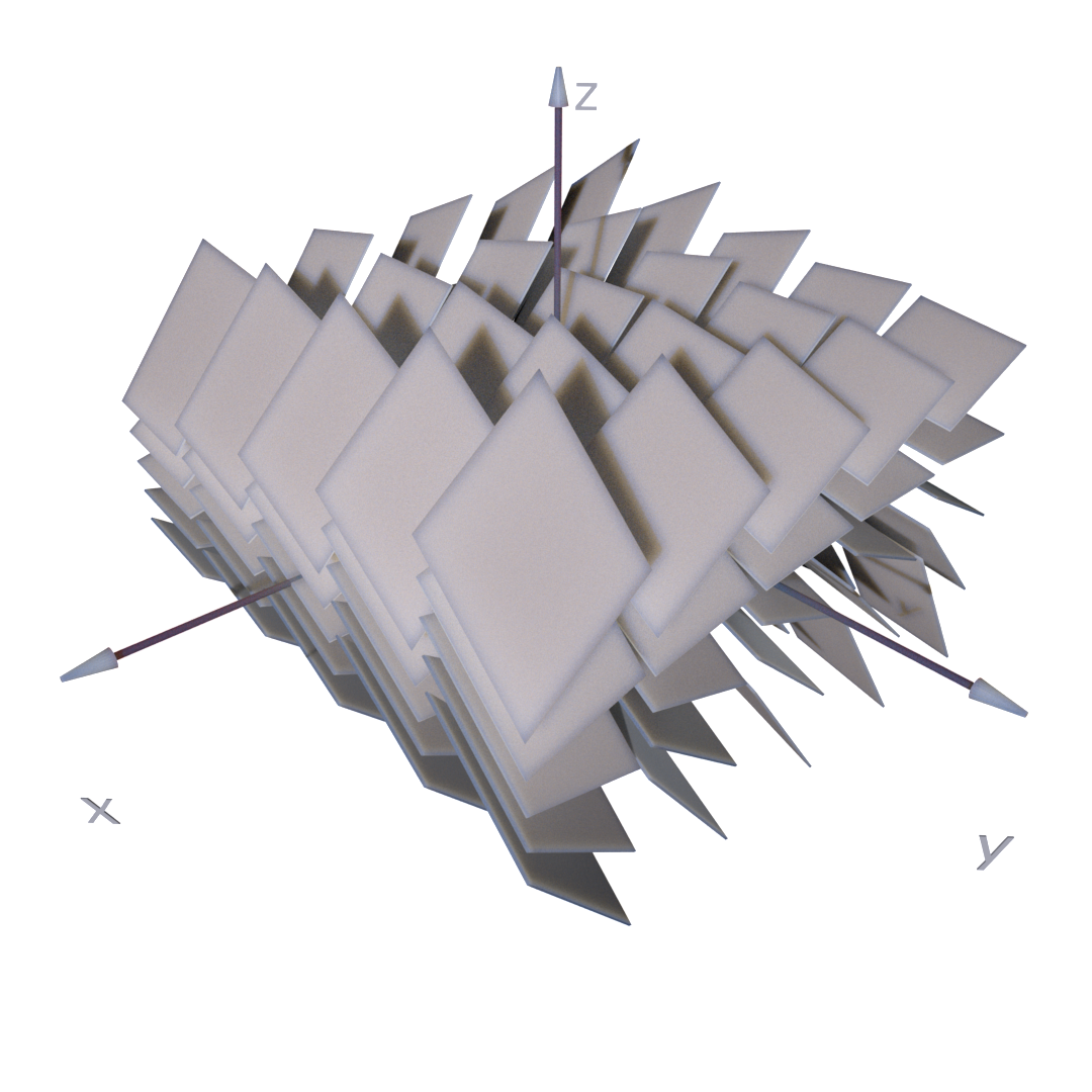
A plane field $\Delta$ in $\mathbb{R}^{3}$ , orthogonal to the vector field $\xi$ , is defined by the equation $\langle\xi,dr\rangle=0$ , where $dr=(dx,dy,dz)$ . See the Figure 2.

If $r=(x,y,z)$ is a singular point of $\xi$ , then the plane of $\Delta$ at $r$ is not defined.

Definition 2.1.

A regular curve $\gamma\colon I\rightarrow\mathbb{R}^{3}$ is an integral curve of a plane field $\Delta$ if $\gamma^{\prime}(t)$ is orthogonal to $\xi(\gamma(t))$ for every $t\in I$ , that is, $\gamma^{\prime}(t)$ is contained in the plane of $\Delta$ at $\gamma(t)$ .

An integral curve of $\Delta$ is also called a Legendre curve of $\Delta$ .

Definition 2.2.

The curl vector field of $\xi$ will be denoted by $curl(\xi)$ , i.e, $curl(\xi)=\left(c_{y}-b_{z},a_{z}-c_{x},b_{x}-a_{y}\right)$ in cartesian coordinates $(x,y,z)$ .

Theorem 2.3 ([2, Jacobi Theorem, p. 2]).

There exist a family of surfaces orthogonal to $\xi$ if, and only if, $\langle\xi,curl(\xi)\rangle\equiv 0$ .

Definition 2.4.

A plane field $\Delta$ is said to be completely integrable if $\langle\xi,curl(\xi)\rangle\equiv 0$ . A surface of the family of surfaces orthogonal to $\xi$ is called an integral surface.

Remark 2.5.

Set the 1-form $\eta=\langle\xi,dr\rangle$ . Then $\eta\wedge d\eta=\langle\xi,curl(\xi)\rangle dx\wedge dy\wedge dz$ . Theorem 2.3 is a special case of the Frobenius Integrability Theorem for differential forms.

2.2. Normal curvature of a plane field

Definition 2.6 ([2, p. 8]).

The normal curvature $k_{n}$ of a plane field, in the direction $dr$ , is defined by

(2.1)

k_{n}=\frac{\langle d^{2}r,\xi\rangle}{\langle dr,dr\rangle}=-\frac{\langle dr,d\xi\rangle}{\langle dr,dr\rangle}.

This definition agrees with the classical one given by L. Euler in [13]. The geometrical interpretation of $k_{n}$ is given by Proposition 2.32.

Proposition 2.7 ([23, Proposition 1.2]).

Let $\Delta$ be a plane field. Then in each plane of $\Delta$ there exists two orthogonal directions at which the normal curvature $k_{n}$ attains the extreme values, minimal and maximal.

Definition 2.8.

The minimal (resp. maximal) principal curvature will be denoted by $k_{1}$ (resp. $k_{2}$ ). The principal direction associated to $k_{1}$ (resp. $k_{2}$ ) will be denoted by $\mathcal{P}_{1}$ (resp. $\mathcal{P}_{2}$ ).

The Euler curvature formula holds for planes fields, see Theorem 2.29:

(2.2)

k_{n}=k_{1}cos^{2}(\theta)+k_{2}sin^{2}(\theta),

where $\theta$ is the angle between $dr$ and the principal direction associated to $k_{1}$ .

2.3. Geodesic curvature and geodesic torsion of a plane field

The geodesic curvature $k_{g}$ of the plane field, in the direction $dr$ , is defined by

(2.3)

k_{g}=\frac{[\xi,dr,d^{2}r]}{\langle dr,dr\rangle^{\frac{3}{2}}}.

See [2, p. 14].

The geodesic torsion $\tau_{g}$ of the plane field, in the direction $dr$ , is defined by

(2.4)

\tau_{g}=\frac{[dr,\xi,d\xi]}{\langle dr,dr\rangle}.

See [2, p. 50]

The geodesic torsion formula for planes fields is given by Theorem 2.33.

2.4. Gaussian curvature and Mean curvature of a plane field

Definition 2.9 ([2, p. 11]).

The Gaussian curvature $\mathcal{K}_{G}$ of a plane field is defined by $\mathcal{K}_{G}=k_{1}k_{2}$ , where $k_{1}$ and $k_{2}$ are the principal curvatures of the plane field.

The Mean curvature $\mathcal{H}_{M}$ of a plane field is defined by $\mathcal{H}_{M}=\frac{k_{1}+k_{2}}{2}$ .

A point $p$ is called, respectively, elliptic, parabolic or hyperbolic when $\mathcal{K}_{G}(p)>0$ , $\mathcal{K}_{G}(p)=0$ or $\mathcal{K}_{G}(p)<0$ .

The set of hyperbolic points (resp. elliptic points) will be denoted by $\mathbb{H}$ (resp. $\mathbb{E}$ ) and is called a hyperbolic region of $\Delta$ (resp. elliptic region of $\Delta$ ). The set of parabolic points will be denoted by $\mathbb{P}$ .

Remark 2.10.

When the plane field is completely integrable, the normal, geodesic curvature and geodesic torsion above coincide with that of curves on surfaces. The definition of the geodesic curvature (resp. geodesic torsion) of a surface can be found in [33, p. 271] and [25, p. 542] (resp. [25, p. 545]).

2.5. Asymptotic lines and parabolic points of a plane field

The directions where $k_{n}=0$ are called asymptotic directions of the plane field and therefore are defined by the following implicit differential equations:

(2.5)

\begin{split}\langle\xi,dr\rangle&=adx+bdy+cdz=0,\\ \langle d\xi,dr\rangle&=a_{x}dx^{2}+(a_{y}+b_{x})dxdy+b_{y}dy^{2}\\ &+(a_{z}+c_{x})dxdz+(b_{z}+c_{y})dydz+c_{z}dz^{2}=0.\end{split}

A solution $dr=(dx,dy,dz)$ of (2.5) is an asymptotic direction. A curve $\gamma$ in $\mathbb{R}^{3}$ is an asymptotic line of the plane field if $\gamma$ is an integral curve of (2.5).

The system (2.5) will be called the implicit differential equation of the asymptotic lines of the plane field.

The line fields of asymptotic directions will be denoted by $\ell_{1}$ and $\ell_{2}$ . They are called asymptotic line fields.

As a consequence of [3, Panov. Corollary of Theorem 4], a closed asymptotic line without parabolic points of a surface in $\mathbb{R}^{3}$ cannot have a convex projection in any plane. See also [9]. However, for plane fields we have no restrictions.

Example 2.11.

The circle in $\mathbb{R}^{3}$ given by $x^{2}+y^{2}=1$ , $z=0$ , is an asymptotic line without parabolic points of the plane field $\Delta$ orthogonal to the vector field $\xi=(a,b,c)$ , where $a=x^{2}yz+y^{3}z-x^{2}y-y^{3}+xz-2yz+y$ , $b=x^{3}-x^{3}z-xy^{2}z+xy^{2}+2xz+yz-x$ and $c=-x^{2}-y^{2}$ . The plane field $\Delta$ is not completely integrable.

The ordered pair $\{\ell_{1},\ell_{2}\}$ is well defined in the hyperbolic region $\mathbb{H}$ , where these directions are real, see the Proposition 2.19.

The asymptotic foliations of $\Delta$ are the integral foliations $\mathcal{A}_{1}$ of $\ell_{1}$ and $\mathcal{A}_{2}$ of $\ell_{2}$ ; they fill out the hyperbolic region $\mathbb{H}$ , see the Proposition 2.19.

Proposition 2.12.

If a straight line is a integral curve of a plane field $\Delta$ , then it is also an asymptotic line of $\Delta$ .

Proof.

Let $\ell(t)=p_{0}+tv$ be a parametrization of the straight line with $v\in\Delta$ . Since $\langle\xi(\ell(t)),v\rangle=0$ it follows that $\langle d\xi(\ell(t))v,v\rangle=0$ . Then the straight line $\ell$ is an asymptotic line of $\Delta$ . ∎

Proposition 2.13.

Given a plane field $\Delta$ , let $h:\mathbb{R}^{3}\rightarrow\mathbb{R}$ be a signal defined smooth function. Then a curve $\gamma$ is an asymptotic line of $\Delta$ if, and only if, $\gamma$ is an asymptotic line of the plane field $\widetilde{\Delta}$ orthogonal to the vector field $\widetilde{\xi}=h\xi$ .

Proof.

The implicit differential equations of the asymptotic lines of $\widetilde{\Delta}$ are given by

(2.6)

\langle\widetilde{\xi},dr\rangle=h\langle\xi,dr\rangle=0,\ \ \langle d\widetilde{\xi}(dr),dr\rangle=dh(dr)\langle\xi,dr\rangle+h\langle d\xi(dr),dr\rangle=0.

Then $\gamma$ is an asymptotic line of $\Delta$ if, and only if, $\gamma$ is an asymptotic line of the plane field $\widetilde{\Delta}$ . ∎

Proposition 2.14.

Let $\gamma$ be a integral curve, parameterized by arc length $s$ , with nonvanishing curvature, of a plane field $\Delta$ and let $\{T,N,B=T\wedge N\}$ be the Frenet orthonormal frame associated to $\gamma$ with the Frenet equations $T^{\prime}=kN$ , $N^{\prime}=-kT+\tau B$ , $B^{\prime}=-\tau N$ , where $k$ is the curvature of $\gamma$ and $\tau$ is the torsion of $\gamma$ . Then $k_{n}^{2}+k_{g}^{2}=k^{2}$ and the following conditions are equivalent:

•

$\gamma$ is an asymptotic line of $\Delta$ .
•

$k_{g}=\pm k$ , where $k_{g}(s)$ is the geodesic curvature 2.3 of $\Delta$ evaluated at the direction of $T(s)$ .
•

for every $s$ , the osculating plane of $\gamma$ at $\gamma(s)$ is the plane of $\Delta$ at $\gamma(s)$ .

Furthermore, if $\gamma$ is an asymptotic line of $\Delta$ , then $\tau_{g}=\tau$ , where $\tau_{g}(s)$ is the geodesic torsion 2.4 of $\Delta$ evaluated at the direction of $T(s)$ .

Proof.

At $\gamma$ , $\xi(s)=cos(\theta(s))N(s)+sin(\theta(s))B(s).$ Then, at $\gamma$ , we have that $d\xi(\gamma^{\prime})=-kcos(\theta)T-(\theta^{\prime}+\tau)sin(\theta)N+(\theta^{\prime}+\tau)cos(\theta)B$ . It follows that the normal 2.1 and geodesic curvatures 2.3, and geodesic torsion 2.4 of $\Delta$ , evaluated at the direction $T$ , are given by $k_{n}=kcos(\theta)$ , $k_{g}=ksin(\theta)$ , $\tau_{g}=\tau+\theta^{\prime}$ and so $k_{n}^{2}+k_{g}^{2}=k^{2}$ . If $\gamma$ is an asymptotic line, which means that $k_{n}=0$ , then $cos(\theta)=0$ and so $sin(\theta)=\pm 1$ , which gives $k_{g}=\pm k$ (or, by the formula $k_{n}^{2}+k_{g}^{2}=k^{2}$ , $k_{g}=\pm k$ ). If $k_{g}=\pm k$ , then $cos(\theta)=0$ and so $\xi=\pm B$ . It follows that, for every $s$ , the osculating plane of $\gamma$ at $\gamma(s)$ is the plane of $\Delta$ at $\gamma(s)$ . If for every $s$ , the osculating plane of $\gamma$ at $\gamma(s)$ is the plane of $\Delta$ at $\gamma(s)$ , then $\xi(s)$ is parallel to $B(s)$ and then $cos(\theta(s))=0$ for every $s$ . It follows that $k_{n}=0$ .

If $\gamma$ is asymptotic line, then $\theta$ is constant, and it follows that $\tau_{g}=\tau$ . ∎

Remark 2.15.

The Proposition 2.14 is the version for plane fields of the equivalent results for surfaces in $\mathbb{R}^{3}$ that are stated, for example, in [39, p. 196].

Lemma 2.16.

Let $\Delta$ be a plane field such that $r=(x,y,z)$ is not a singular point of $\xi=(a,b,c)$ . Then we can choose a coordinate system such that $c(r)\neq 0$ . In this coordinate system, the implicit differential equations of the asymptotic lines, in a neighbourhood of $r$ , becomes

(2.7)

\begin{split}dz=-\left(\frac{a}{c}\right)dx-\left(\frac{b}{c}\right)dy,\quad edx^{2}+2fdxdy+gdy^{2}=0,\end{split}

where

(2.8)

\begin{split}e&=a_{x}-\frac{(a_{z}+c_{x})a}{c}+\frac{a^{2}c_{z}}{c^{2}},\ \ g=b_{y}-\frac{(b_{z}+c_{y})b}{c}+\frac{b^{2}c_{z}}{c^{2}},\\ f&=\frac{a_{y}+b_{x}}{2}-\frac{(a_{z}+c_{x})b}{2c}-\frac{(b_{z}+c_{y})a}{2c}+\frac{abc_{z}}{c^{2}}.\end{split}

Furthermore, in this neighbourhood, the parabolic set of $\Delta$ is given by $eg-f^{2}=0$ .

Proof.

Since $\xi(r)\neq(0,0,0)$ , we can choose a coordinate system such that $c(r)\neq 0$ . In a neighbourhood of $r$ , the equation $\langle\xi,dr\rangle=0$ of (2.5) can be solved for $dz$ and then we get the first equation of (2.7). Replace this $dz$ on the equation $\langle d\xi,dr\rangle=0$ of (2.5) to get the second equation of (2.7).

By (2.7), at a point $(x,y,z)$ , all directions are asymptotic directions if, and only if, $e(x,y,z)=f(x,y,z)=g(x,y,z)=0$ and, at a point $(x,y,z)$ , the asymptotic directions coincides if, and only if, $e(x,y,z)g(x,y,z)-(f(x,y,z))^{2}=0$ . ∎

Definition 2.17.

Let $\Delta$ be a plane field satisfying the assumptions of the Lemma 2.16. Set $\mathcal{K}=eg-f^{2}$ and $\mathcal{H}=-\left(\frac{e+g}{2}\right)$ .

Proposition 2.18 ([2, p. 11]).

Let $\Delta$ be a plane field satisfying the assumptions of the Lemma 2.16.

•

$\mathcal{K}(0,0,0)=\mathcal{K}_{G}(0,0,0)$ and $\mathcal{H}(0,0,0)=\mathcal{H}_{M}(0,0,0)$ ,
•

$\mathcal{K}=0$ if, and only if, $\mathcal{K}_{G}=0$ and $\mathcal{H}=0$ if, and only if, $\mathcal{H}_{M}=0$ .

Proposition 2.19.

The asympotic directions are well defined in the hyperbolic region $\mathbb{H}$ , the directions are real. The asymptotic foliations fill out the hyperbolic region $\mathbb{H}$ . Locally, the asymptotic lines in $\mathbb{H}$ are as show in the Figure 3.

Proof.

Let $r=(x,y,z)$ be a point of a open subset of $\mathbb{H}$ . By Lemma 2.16, the implicit differential equations of the asymptotic lines, in a neighbourhood of $r$ , are given by (2.7). Since $r\in\mathbb{H}$ , in a neighbourhood $\Lambda$ of $r$ , the functions $e$ , $f$ , $g$ does not vanishes simultaneously. Without loss of generality, suppose that $e$ does not vanishes at $\Lambda$ . Then we can solve the equation $edx^{2}+2fdxdy+gdy^{2}=0$ for $dy$ to get

(2.9)

dy=\left(\frac{-f\pm\sqrt{-\mathcal{K}}}{e}\right)dx.

By (2.7),

(2.10)

dz=\left[-\left(\frac{a}{c}\right)-\left(\frac{-bf\pm b\sqrt{-\mathcal{K}}}{ce}\right)\right]dx.

This defines the following two vector fields $Z_{+}(x,y,z)$ and $Z_{-}(x,y,z)$ in $\Lambda$ :

(2.11)

Z_{\pm}=\left(1,\frac{dy}{dx},\frac{dz}{dx}\right)=\left(1,\left(\frac{-f\pm\sqrt{-\mathcal{K}}}{e}\right),-\left(\frac{a}{c}\right)-\left(\frac{-bf\pm b\sqrt{-\mathcal{K}}}{ce}\right)\right).

Since $\mathcal{K}$ never vanishes, then, at each point of $\Lambda$ , the integral curves of $Z_{+}$ and $Z_{-}$ are transversal. ∎

Remark 2.20.

We can apply the Tubular Flow Theorem (see, for example, [32, Tubular Flow Theorem, p. 40]) for one of the vector fields $Z_{\pm}$ , but we cannot apply it directly for both vector fields simultaneously.

Remark 2.21.

The Proposition 2.19 is the version for asymptotic lines of plane fields of the [27, Theorem 2.2, p. 166].

Lemma 2.22.

Let $\Delta$ be a plane field satisfying the assumptions of Lemma 2.16. If $(0,0,0)\in\mathbb{H}\cup\mathbb{P}$ , then in a neighbourhood of $(0,0,0)$ , $\xi=(a,b,c)$ where

(2.12)

\begin{split}a&=a_{2}y+a_{3}z+(a_{11}x^{2}+a_{12}xy+a_{13}xz+a_{22}y^{2}+a_{23}yz+a_{33}z^{2})\\ &+(a_{111}x^{3}+a_{112}x^{2}y+a_{113}x^{2}z+a_{122}xy^{2}+a_{123}xyz+a_{133}xz^{2}+a_{222}y^{3}\\ &+a_{223}y^{2}z+a_{233}yz^{2}+a_{333}z^{3})+\sum_{i+j+k=4}a_{ij}^{k}x^{i}y^{j}z^{k}+\mathcal{O}^{5}(x,y,z),\\ b&=b_{1}x+b_{2}y+b_{3}z+(b_{11}x^{2}+b_{12}xy+b_{13}xz+b_{22}y^{2}+b_{23}yz+b_{33}z^{2})\\ &+(b_{111}x^{3}+b_{112}x^{2}y+b_{113}x^{2}z+b_{122}xy^{2}+b_{123}xyz+b_{133}xz^{2}+b_{222}y^{3}\\ &+b_{223}y^{2}z+b_{233}yz^{2}+b_{333}z^{3})+\sum_{i+j+k=4}b_{ij}^{k}x^{i}y^{j}z^{k}+\mathcal{O}^{5}(x,y,z),\\ c&=1+(c_{11}x^{2}+c_{12}xy+c_{13}xz+c_{22}y^{2}+c_{23}yz+c_{33}z^{2})\\ &+(c_{111}x^{3}+c_{112}x^{2}y+c_{113}x^{2}z+c_{122}xy^{2}+c_{123}xyz+c_{133}xz^{2}+c_{222}y^{3}\\ &+c_{223}y^{2}z+c_{233}yz^{2}+c_{333}z^{3})+\sum_{i+j+k=4}c_{ij}^{k}x^{i}y^{j}z^{k}+\mathcal{O}^{5}(x,y,z).\end{split}

Furthermore, the implicit differential equation of the asymptotic lines evaluated at $(0,0,0)$ are given by

(2.13)

dz=0,\ \ (a_{2}+b_{1})dxdy+b_{2}dy^{2}=0.

$\mathcal{K}(0,0,0)=-(a_{2}+b_{1})^{2}$ and

(2.14)

\nabla\mathcal{K}(0,0,0)=(2b_{2}a_{11},(a_{3}b_{1}+a_{12})b_{2},[a_{13}-(a_{3})^{2}]b_{2}).

Proof.

By the Proposition 2.13 we can suppose that $\xi$ is unitary. By Lemma 2.16, we can choose a coordinate system in $\mathbb{R}^{3}$ such that $c(0,0,0)\neq 0$ . Moreover, without loss of generality, this coordinate system can be taken such that $\xi(0,0,0)=(0,0,1)$ . Then $c_{x}(0,0,0)=c_{y}(0,0,0)=c_{z}(0,0,0)=0$ . By 2.16, the implicit differential equation of the asymptotic lines evaluated at $(0,0,0)$ becomes

(2.15)

dz=0,\ \ a_{x}(0,0,0)dx^{2}+\left(\frac{a_{y}(0,0,0)+b_{x}(0,0,0)}{2}\right)dxdy+b_{y}(0,0,0)dy^{2}=0.

There is a rotation in $\mathbb{R}^{3}$ around the $z$ axis that makes $(dx,0,0)$ be one asymptotic direction at $(0,0,0)$ , that is, $a_{x}(0,0,0)=0$ . It follows that $\xi=(a,b,c)$ , where $a$ , $b$ and $c$ are given by (2.12) and that the implicit differential equations of the asymptotic lines (2.7) evaluated at $(0,0,0)$ are given by (2.13).

Then, $e(0,0,0)=0$ , $f(0,0,0)=a_{2}+b_{1}$ , $g(0,0,0)=b_{2}$ and $\mathcal{K}(0,0,0)=-(a_{2}+b_{1})^{2}$ . ∎

Remark 2.23.

In [2] there is defined the following Mean curvature of first kind: $\mathcal{H}_{1}=-\left(\frac{a_{x}+b_{y}}{2}\right)$ , related with the divergence of the vector field $\xi$ . It follows that $\mathcal{H}\neq\mathcal{H}_{1}$ , but $\mathcal{H}(0,0,0)=\mathcal{H}_{1}(0,0,0)$ .

Proposition 2.24.

If $(0,0,0)\in\mathbb{P}$ , then $a_{2}=-b_{1}$ . If $b_{2}\neq 0$ , then at $(0,0,0)$ the two asymptotic directions coincides with the asymptotic direction $\mathcal{A}=\left(dx,0,0\right)$ , $dx\neq 0$ , where, without loss of generality, we can assume $dx=1$ . If $b_{2}=0$ , then at $(0,0,0)$ , all directions in the plane of $\Delta$ at $(0,0,0)$ are asymptotic directions.

Proof.

By Lemma 2.22, $\xi=(a,b,c)$ where $a$ , $b$ and $c$ are given by (2.12). The implicit differential equations of the asymptotic lines (2.7) evaluated at $(0,0,0)$ are given by (2.13). Since $\mathcal{K}(0,0,0)=-(a_{2}+b_{1})^{2}$ , it follows that $a_{2}=-b_{1}$ . The equations (2.13) becomes $dz=0$ , $b_{2}dy^{2}=0$ . If $b_{2}\neq 0$ , then the asymptotic direction at $(0,0,0)$ is given by $\mathcal{A}=(dx,0,0)$ . If $b_{2}=0$ , then all the directions $(dx,dy,0)$ are asymptotic directions. Note that the plane of $\Delta$ at $(0,0,0)$ is given by $dz=0$ . ∎

2.6. Principal directions

The principal directions of a plane field $\Delta$ are defined by the following system of implicit differential equations, see [2] and [24]:

(2.16)

\langle\xi,dr\rangle=0,\ \ 2[d\xi,dr,\xi]+\langle curl(\xi),\xi\rangle\langle dr,dr\rangle=0.

Definition 2.25.

The equations (2.16) are said to be the implicit differential equations of the principal curvature lines of $\Delta$ .

Definition 2.26.

A solution $dr=(dx,dy,dz)$ of (2.16) is called of principal direction of $\Delta$ . A curve $\gamma$ in $\mathbb{R}^{3}$ is a principal curvature line of $\Delta$ if $\gamma$ is a integral curve of (2.16).

Remark 2.27.

If $(x,y,z)$ is a singular point of $\xi$ , then the principal directions are not defined in $(x,y,z)$ .

Proposition 2.28.

The second equation of (2.16) is equivalent to $2\tau_{g}+\langle curl(\xi),\xi\rangle=0$ . Furthermore, let $\tau_{g,i}$ , $i=1,2$ , be the geodesic torsion evaluated at the principal direction associated to the principal curvature $k_{i}$ . Then $\tau_{g,1}=\tau_{g,2}$ .

Proof.

By the definition of geodesic torsion 2.4, it is clear that the second equation of (2.16) is equivalent to $2\tau_{g}+\langle curl(\xi),\xi\rangle=0$ . It follows from the two equations $2\tau_{g,i}+\langle curl(\xi),\xi\rangle=0$ , $i=1,2$ , that $\tau_{g,1}-\tau_{g,2}=0$ . ∎

Theorem 2.29 (Euler curvature formula for a plane field).

Let $\Delta$ be a plane field, then

(2.17)

k_{n}=k_{1}cos^{2}(\theta)+k_{2}sin^{2}(\theta),

where $\theta$ is the angle between the direction $dr$ and the principal direction associated with $k_{1}$ .

Proof.

The proof given in [13] holds for plane fields. For different proofs, see [2, p. 12] and the Section 2.8. ∎

Proposition 2.30.

[2, Section 1.2] The equation (2.16) defines two principal directions at every point that is not a partially umbilic point. At a partially umbilic point, all directions are principal directions.

Proposition 2.31.

If $(0,0,0)\in\mathbb{P}$ , then one asymptotic direction at $(0,0,0)$ is a principal direction.

Proof.

In $(0,0,0)$ the implicit differential equations of the principal curvatures lines of the plane field $\Delta$ are given by $b_{2}dxdy=0$ and $dz=0$ and then one principal direction in $(0,0,0)$ is given by $(dx,0,0)=\mathcal{A}$ . If $b_{2}=0$ , then all directions in $\Delta$ are principal directions and then $(0,0,0)$ is a partially umbilic point of $\Delta$ . ∎

2.7. Geometrical interpretation of the normal curvature of a plane field

Proposition 2.32.

The normal curvature $k_{n}$ of a plane field $\Delta$ evaluated at a point $P$ and in the direction $dr$ is the curvature $k$ , evaluated at $P$ , of a plane curve $\gamma$ , which is the integral curve of the line field $\ell$ defined by the intersection of the plane $\mathcal{N}$ generated by $dr$ and $\xi(P)$ with the plane field $\Delta$ , see the Figure 4.

Proof.

There is no loss of generality in assuming that $\langle dr,dr\rangle=1$ and that $\xi$ is unitary. Let $\zeta^{\bot}$ be the projection of $\xi$ onto the plane $\mathcal{N}$ :

(2.18)

\zeta^{\bot}(x,y,z)=\xi(x,y,z)-\langle\xi(x,y,z),(\xi(P)\wedge dr)\rangle(\xi(P)\wedge dr).

Let $\zeta$ be the vector field at $\mathcal{N}$ orthogonal to $\zeta^{\bot}$ , that is, $\langle\zeta^{\bot},\zeta\rangle\equiv 0$ and $\langle(\xi(P)\wedge dr),\zeta\rangle\equiv 0$ . By equation (2.18), we have that $\langle\xi,\zeta\rangle\equiv 0$ . It follows that $\zeta$ defines the straight line field $\ell$ and $\zeta(P)$ is parallel to $dr$ . Now, $\gamma$ is a curve such that $\gamma(0)=P$ , $\gamma^{\prime}(t)=\zeta(\gamma(t))$ and $\gamma^{\prime}(0)=dr$ . It follows that the normal vector of $\gamma$ at $P$ is $\xi(P)$ and, at $\gamma$ , $\langle\xi,\gamma^{\prime}\rangle\equiv 0$ . Then the curvature $k$ of $\gamma$ at $P$ is given by $k=\langle\xi(P),\gamma^{\prime\prime}(0)\rangle$ . Since $\langle\xi(\gamma),\gamma^{\prime}\rangle\equiv 0$ , then, at $\gamma$ , $\langle\xi,\gamma^{\prime\prime}\rangle=-\langle d\xi(\gamma^{\prime}),\gamma^{\prime}\rangle$ . Then, at $P$ ,

(2.19)

k=-\langle d\xi(\gamma^{\prime}(0)),\gamma^{\prime}(0)\rangle=-\langle d\xi(dr),dr\rangle=k_{n},

where $k_{n}$ is the normal curvature defined by equation (2.1), evaluated at $P$ in the direction $dr$ . ∎

2.8. Darboux frame

Let $\gamma:I\rightarrow\mathbb{R}^{3}$ be a integral curve of a plane field $\Delta$ , parametrized by arc lenght $s$ . The Darboux frame $\{X(s),Y(s),(X\wedge Y)(s)=\xi(s)\}$ associated to $\gamma$ , where $\gamma^{\prime}(s)=X(s)$ , $\langle X(s),Y(s)\rangle=0$ , $\langle Y(s),Y(s)\rangle=1$ , $\langle(X\wedge Y)(s),(X\wedge Y)(s)\rangle=1$ , is defined by the equations:

(2.20)

\begin{split}\left.\nabla_{X}X\right|_{\gamma(s)}&=k_{g}(s)Y(s)+k_{n}(s)(X\wedge Y)(s),\\ \left.\nabla_{X}Y\right|_{\gamma(s)}&=-k_{g}(s)X(s)+\tau_{g}(s)(X\wedge Y)(s),\\ \left.\nabla_{X}(X\wedge Y)\right|_{\gamma(s)}&=-k_{n}(s)X(s)-\tau_{g}(s)Y(s),\end{split}

where $k_{n}$ , $k_{g}$ and $\tau_{g}$ are the normal curvature (2.1), geodesic curvature (2.3) and geodesic torsion (2.4) of the plane field $\Delta$ in the direction $X$ :

(2.21)

\begin{split}k_{n}(s)&=\langle\left.\nabla_{X}X\right|_{\gamma(s)},(X\wedge Y)(s)\rangle=-\langle X(s),\left.\nabla_{X}(X\wedge Y)\right|_{\gamma(s)}\rangle,\\ k_{g}(s)&=((X\wedge Y)(s),X(s),\left.\nabla_{X}X\right|_{\gamma(s)})\\ &=\langle Y(s),\left.\nabla_{X}X\right|_{\gamma(s)}\rangle=-\langle\left.\nabla_{X}Y\right|_{\gamma(s)},X(s)\rangle,\\ \tau_{g}(s)&=(X(s),(X\wedge Y)(s),\left.\nabla_{X}(X\wedge Y)\right|_{\gamma(s)})\\ &=-\langle Y(s),\left.\nabla_{X}(X\wedge Y)\right|_{\gamma(s)}\rangle=\langle\left.\nabla_{X}Y\right|_{\gamma(s)},(X\wedge Y)(s)\rangle.\end{split}

Also, at $\gamma(s)$ , we have that

(2.22)

\begin{split}\left.\nabla_{Y}Y\right|_{\gamma(s)}&=-k_{g,Y}(s)X(s)+k_{n,Y}(s)(X\wedge Y)(s),\\ \left.\nabla_{Y}X\right|_{\gamma(s)}&=k_{g,Y}(s)Y(s)-\tau_{g,Y}(s)(X\wedge Y)(s),\\ \left.\nabla_{Y}(X\wedge Y)\right|_{\gamma(s)}&=\tau_{g,Y}(s)X(s)-k_{n,Y}(s)Y(s),\end{split}

where $k_{n,Y}$ , $k_{g,Y}$ and $\tau_{g,Y}$ are the normal curvature (2.1), geodesic curvature (2.3) and geodesic torsion (2.4) of the plane field $\Delta$ , at $\gamma(s)$ , in the direction $Y$ .

Theorem 2.33.

Let $\Delta$ be a plane field. Then

(2.23)

\tau_{g}-\widetilde{\tau}_{g}=(k_{2}-k_{1})cos(\theta)sin(\theta),

where $k_{1}$ and $k_{2}$ are the principal curvatures of $\Delta$ , $\theta$ is the angle between the direction $dr$ and the principal direction associated to $k_{1}$ and $\widetilde{\tau}_{g}$ is the geodesic torsion evaluated in the principal direction.

Remark 2.34.

The version of the Theorem 2.33 for surfaces in $\mathbb{R}^{3}$ , see for example [39, Proposition 2, p.192], states that $\tau_{g}=(k_{2}-k_{1})cos(\theta)sin(\theta)$ . This difference happens because, at surfaces, $\tau_{g,1}=\tau_{g,2}=0$ , see for example [39, p. 196].

Proof of the Theorems 2.29 and 2.33.

At a point $(x,y,z)$ , let $\gamma$ be a integral curve of $\Delta$ , parametrized by arc length $s$ , such that $\gamma(0)=(x,y,z)$ . Consider the Darboux frame $\{X(s),Y(s),(X\wedge Y)(s)=\xi(s)\}$ associated to $\gamma$ , where $\gamma^{\prime}(s)=X(s)$ . At $\gamma$ , $X=cos(\theta)X_{1}+sin(\theta)X_{2}$ and so $Y=-sin(\theta)X_{1}+cos(\theta)X_{2}$ , where at a point $\gamma(s)$ , $X_{1}(s)$ and $X_{2}(s)$ are the two principal directions at it. It follows that

(2.24)

\begin{split}\left.\nabla_{X}(X\wedge Y)\right|_{\gamma(s)}&=cos(\theta)\left.\nabla_{X_{1}}(X\wedge Y)\right|_{\gamma(s)}+sin(\theta)\left.\nabla_{X_{2}}(X\wedge Y)\right|_{\gamma(s)}\\ &=cos(\theta)\left.\nabla_{X_{1}}(X_{1}\wedge X_{2})\right|_{\gamma(s)}+sin(\theta)\left.\nabla_{X_{2}}(X_{1}\wedge X_{2})\right|_{\gamma(s)}.\end{split}

By (2.20), $\left.\nabla_{X_{1}}(X_{1}\wedge X_{2})\right|_{\gamma(s)}=-k_{1}X_{1}-\tau_{g,1}X_{2}$ , where $k_{1}$ is the principal direction associated with $X_{1}$ and $\tau_{g,1}$ is the geodesic torsion evaluated in the direction $X_{1}$ . By (2.22), $\left.\nabla_{X_{2}}(X_{1}\wedge X_{2})\right|_{\gamma(s)}=-k_{2}X_{2}+\tau_{g,2}X_{1}$ , where $k_{2}$ is the principal direction associated with $X_{2}$ and $\tau_{g,2}$ is the geodesic torsion evaluated in the direction $X_{2}$ .

By Proposition 2.28, it follows that $\widetilde{\tau}_{g}=\tau_{g,1}=\tau_{g,2}$ .

Then $k_{n}(s)=-\langle X(s),\left.\nabla_{X}(X\wedge Y)\right|_{\gamma(s)}\rangle=k_{1}cos^{2}(\theta)+k_{2}sin^{2}(\theta)$ , which prove the Theorem 2.29 and $\tau_{g}(s)=-\langle Y(s),\left.\nabla_{X}(X\wedge Y)\right|_{\gamma(s)}\rangle=(k_{2}-k_{1})cos(\theta)sin(\theta)+\widetilde{\tau}_{g}$ , which prove the Theorem 2.33. ∎

Remark 2.35.

The Euler curvature formula (2.17) and the formula (2.23) are equivalent to the formulas [38, 3 and 4, p. 105] respectively.

2.8.1. Triple orthogonal system of plane fields

With the notation above, we have that

(2.25)

\begin{split}\left.\nabla_{X\wedge Y}(X\wedge Y)\right|_{\gamma(s)}&=l_{1}(s)X(s)+l_{2}(s)Y(s)\\ \left.\nabla_{X\wedge Y}X\right|_{\gamma(s)}&=l_{3}(s)Y(s)-l_{1}(s)(X\wedge Y)(s),\\ \left.\nabla_{X\wedge Y}Y\right|_{\gamma(s)}&=-l_{3}(s)X(s)-l_{2}(s)(X\wedge Y)(s).\\ \end{split}

Let $\Delta_{X}$ and $\Delta_{Y}$ be plane fields such that $\{\Delta,\Delta_{X},\Delta_{Y}\}$ is a triple orthogonal system of plane fields and, for all $s$ , the vector orthogonal to $\Delta_{X}$ (resp. $\Delta_{Y}$ ) at $\gamma(s)$ is $X(s)$ (resp. $Y(s)$ ).

Let $k_{n}^{\Delta_{X}}$ , $k_{g}^{\Delta_{X}}$ , $\tau_{g}^{\Delta_{X}}$ (resp. $k_{n}^{\Delta_{Y}}$ , $k_{g}^{\Delta_{Y}}$ , $\tau_{g}^{\Delta_{Y}}$ ) be respectively the normal curvature, geodesic curvature and geodesic torsion of the plane field $\Delta_{X}$ (resp. $\Delta_{Y}$ ) evaluated at the direction $X\wedge Y$ . It follows, directly from the definitions 2.1, 2.3, 2.4, that $l_{1}=k_{n}^{\Delta_{X}}=k_{g}^{\Delta_{Y}}$ , $l_{2}=k_{n}^{\Delta_{Y}}=-k_{g}^{\Delta_{X}}$ and $l_{3}=\tau_{g}^{\Delta_{X}}=\tau_{g}^{\Delta_{Y}}$ .

2.9. The second fundamental form of a plane field

Let $\{X,Y\}$ be a local basis for the plane field $\Delta$ , that is, locally, $X\wedge Y=\xi$ .

Definition 2.36 ([36]).

The second fundamental form $II$ of $\Delta$ is defined by

(2.26)

II(X,Y)=\frac{1}{2}\langle\nabla_{X}Y+\nabla_{Y}X,\xi\rangle.

Remark 2.37 ([36]).

In the case that $\Delta$ is completely integrable, $II$ is the second fundamental form of the integral surfaces.

Proposition 2.38.

Let $X_{i}$ , $i=1,2$ , be the principal direction associated with $k_{i}$ . Then $II(X_{1},X_{2})=0$ and

(2.27)

\frac{II(X_{1},X_{1})}{\langle X_{1},X_{1}\rangle}=k_{1},\ \ \frac{II(X_{2},X_{2})}{\langle X_{2},X_{2}\rangle}=k_{2}.

Proof.

The principal curvatures $k_{i}$ , $i=1,2$ , are given by $k_{i}=\frac{\langle\nabla_{X_{i}}X_{i},\xi\rangle}{\langle X_{i},X_{i}\rangle}$ . It follows that $\frac{II(X_{i},X_{i})}{\langle X_{i},X_{i}\rangle}=k_{i}$ . The geodesic torsion evaluated at the direction $X_{1}$ (resp. $X_{2}$ ) is given by $\tau_{g,1}=\frac{\langle\nabla_{X_{1}}X_{2},\xi\rangle}{\langle X_{1},X_{1}\rangle}$ (resp. $\tau_{g,2}=-\frac{\langle\nabla_{X_{2}}X_{1},\xi\rangle}{\langle X_{2},X_{2}\rangle}$ ). It follows that $\frac{II(X_{1},X_{2})}{\langle X_{1},X_{1}\rangle\langle X_{2},X_{2}\rangle}=\frac{\tau_{g,1}-\tau_{g,2}}{2}$ . By Proposition 2.28, $\tau_{g,1}-\tau_{g,2}=0$ and then $II(X_{1},X_{2})=0$ . ∎

Remark 2.39.

The [29, Lemma 2.4, item 3] asserts that $II(X_{1},X_{2})=0$ if $X_{1}$ , $X_{2}$ are the principal directions and can be used to prove the Proposition 2.38.

Theorem 2.40.

The following holds

(2.28)

\begin{split}\mathcal{K}_{G}&=\frac{II(X,X)II(Y,Y)-(II(X,Y))^{2}}{\langle X,X\rangle\langle Y,Y\rangle-\langle X,Y\rangle^{2}},\\ \mathcal{H}_{M}&=\frac{II(X,X)\langle Y,Y\rangle-2II(X,Y)\langle X,Y\rangle+II(Y,Y)\langle X,X\rangle}{2(\langle X,X\rangle\langle Y,Y\rangle-\langle X,Y\rangle^{2})},\end{split}

where $\mathcal{K}_{G}$ (resp. $\mathcal{H}_{M}$ ) is the Gauss curvature (resp. Mean curvature) of $\Delta$ .

Proof.

We can write $X$ and $Y$ as

(2.29)

X=cos(\theta)X_{1}+sin(\theta)X_{2},\ \ Y=cos(\alpha)X_{1}+sin(\alpha)X_{2},

where $X_{i}$ , $i=1,2$ , is the principal direction associated to $k_{i}$ . It follows that

(2.30)

\begin{split}\langle X,X\rangle&=\langle X_{1},X_{1}\rangle cos^{2}(\theta)+\langle X_{2},X_{2}\rangle sin^{2}(\theta),\\ \langle Y,Y\rangle&=\langle X_{1},X_{1}\rangle cos^{2}(\alpha)+\langle X_{2},X_{2}\rangle sin^{2}(\alpha),\\ \langle X,Y\rangle&=\langle X_{1},X_{1}\rangle cos(\theta)cos(\alpha)+\langle X_{2},X_{2}\rangle sin(\theta)sin(\alpha).\end{split}

Then

(2.31)

\langle X,X\rangle\langle Y,Y\rangle-\langle X,Y\rangle^{2}=(cos(\theta)sin(\alpha)-cos(\alpha)sin(\theta))^{2}\langle X_{1},X_{1}\rangle\langle X_{2},X_{2}\rangle,

and

(2.32)

\begin{split}II(X,X)&=II(X_{1},X_{1})cos^{2}(\theta)+2II(X_{1},X_{2})cos(\theta)sin(\theta)+II(X_{2},X_{2})sin^{2}(\theta),\\ II(Y,Y)&=II(X_{1},X_{1})cos^{2}(\alpha)+2II(X_{1},X_{2})cos(\alpha)sin(\alpha)+II(X_{2},X_{2})sin^{2}(\alpha),\\ II(X,Y)&=II(X_{1},X_{1})cos(\theta)cos(\alpha)+II(X_{1},X_{2})(cos(\theta)sin(\alpha)+cos(\alpha)sin(\theta))\\ &+II(X_{2},X_{2})sin(\theta)sin(\alpha).\end{split}

It follows that

(2.33)

\frac{II(X,X)II(Y,Y)-(II(X,Y))^{2}}{\langle X,X\rangle\langle Y,Y\rangle-\langle X,Y\rangle^{2}}=\frac{II(X_{1},X_{1})II(X_{2},X_{2})-(II(X_{1},X_{2}))^{2}}{\langle X_{1},X_{1}\rangle\langle X_{2},X_{2}\rangle},

and

(2.34)

\begin{split}&\frac{II(X,X)\langle Y,Y\rangle-2II(X,Y)\langle X,Y\rangle+II(Y,Y)\langle X,X\rangle}{2(\langle X,X\rangle\langle Y,Y\rangle-\langle X,Y\rangle^{2})}\\ &=\frac{II(X_{1},X_{1})\langle X_{2},X_{2}\rangle+II(X_{2},X_{2})\langle X_{1},X_{1}\rangle}{2\langle X_{1},X_{1}\rangle\langle X_{2},X_{2}\rangle}.\end{split}

By Proposition 2.38, $\frac{II(X_{1},X_{1})}{\langle X_{1},X_{1}\rangle}=k_{1}$ and $\frac{II(X_{2},X_{2})}{\langle X_{2},X_{2}\rangle}=k_{2}$ . ∎

Remark 2.41.

The Mean curvature $\mathcal{H}_{M}$ of a plane field as the expression given in (2.28) is defined in [36]. The expression of $\mathcal{K}_{G}$ of (2.28) is defined in [28, Definition 2.5], where is called of sectional curvature of the plane field.

2.10. Tubular neighbourhood around an integral curve of the plane field

Let $\gamma$ be a integral curve of the plane field $\Delta$ , parametrized by arc lenght $u$ .

Set $X(u)=\gamma^{\prime}(u)$ and consider the Darboux frame defined in Section 2.8 with the equations (2.20), (2.22) and (2.25).

By Theorems 2.29 and 2.33,

(2.35)

\begin{split}k_{n}(u)&=k_{1}(u)cos^{2}(\theta(u))+k_{2}(u)sin^{2}(\theta(u)),\\ \tau_{g}(u)&=\widetilde{\tau}_{g}(u)+(k_{1}(u)-k_{2}(u))cos(\theta(u))sin(\theta(u)).\end{split}

Since $\langle X(u),Y(u)\rangle=0$ for all $u$ , then

(2.36)

\begin{split}k_{n,Y}(u)&=k_{1}(u)sin^{2}(\theta(u))+k_{2}(u)cos^{2}(\theta(u)),\\ \tau_{g,Y}(u)&=\widetilde{\tau}_{g}(u)-(k_{1}(u)-k_{2}(u))cos(\theta(u))sin(\theta(u)).\end{split}

Let $\alpha:\Lambda\subset\mathbb{R}^{3}\rightarrow\mathbb{R}^{3}$ defined by

(2.37)

\alpha(u,v,w)=\gamma(u)+vY(u)+w(X\wedge Y)(u),

where $\Lambda$ is a open subset.

Definition 2.42.

The map $\alpha$ is a tubular neighbourhood around the integral curve $\gamma$ .

Lemma 2.43.

In the tubular neighbourhood around an integral curve of the plane field, $\mathcal{K}=\mathcal{K}_{G}$ and $\mathcal{H}=\mathcal{H}_{M}$ .

Proof.

Since $d\alpha=\alpha_{u}du+\alpha_{v}dv+\alpha_{w}dw$ , then

(2.38)

d\alpha=[(1-vk_{g}-wk_{n})du]X+[dv-w\tau_{g}du]Y+[v\tau_{g}du+dw]X\wedge Y.

Since $\xi(u,0,0)=(X\wedge Y)(u)$ , at the tubular neighbourhood $\alpha$ , the Taylor expansion of $\xi$ is given by

(2.39)

\begin{split}&\xi(u,v,w)=(X\wedge Y)(u,0,0)+v\left.\nabla_{Y}(X\wedge Y)\right|_{\gamma(u)}+w\left.\nabla_{X\wedge Y}(X\wedge Y)\right|_{\gamma(u)}\\ &+\Bigg(\frac{v^{2}m_{11}(u)}{2}+vwm_{21}(u)+\frac{w^{2}m_{31}(u)}{2}+\frac{n_{11}(u)v^{3}}{6}+\frac{n_{21}(u)v^{2}w}{2}+\frac{n_{31}(u)vw^{2}}{2}\\ &+\frac{n_{41}(u)w^{3}}{6}+\mathcal{O}^{4}_{u}(v,w)\Bigg)X(u)+\Bigg(\frac{v^{2}m_{12}(u)}{2}+vwm_{22}(u)+\frac{w^{2}m_{32}(u)}{2}\\ &+\frac{n_{12}(u)v^{3}}{6}+\frac{n_{22}(u)v^{2}w}{2}+\frac{n_{32}(u)vw^{2}}{2}+\frac{n_{42}(u)w^{3}}{6}+\mathcal{O}^{4}_{u}(v,w)\Bigg)Y(u)\\ &+\Bigg(\frac{v^{2}m_{13}(u)}{2}+vwm_{23}(u)+\frac{w^{2}m_{33}(u)}{2}+\frac{n_{13}(u)v^{3}}{6}+\frac{n_{23}(u)v^{2}w}{2}+\frac{n_{33}(u)vw^{2}}{2}\\ &+\frac{n_{43}(u)w^{3}}{6}+\mathcal{O}^{4}_{u}(v,w)\Bigg)(X\wedge Y)(u).\end{split}

We have that $d\xi=\xi_{u}du+\xi_{v}dv+\xi_{w}dw$ . The implicit differential equations (2.5) of the asymptotic lines are given by $\langle\xi,d\alpha\rangle=0$ and $\langle d\xi,d\alpha\rangle=0$ . We can solve the equation $\langle\xi,d\alpha\rangle=0$ for $dw$ and substitute it in $\langle d\xi,d\alpha\rangle=0$ . Then the equations of the asymptotic lines becomes $dw=Adu+Bdv$ and $edu^{2}+2fdudv+gdv^{2}=0$ , where

(2.40)

\begin{split}e(u,v,w)&=-k_{n}(u)+\mathcal{O}^{1}_{u}(v,w),\quad f(u,v,w)=-\frac{\tau_{g}(u)-\tau_{g,Y}(u)}{2}+\mathcal{O}^{1}_{u}(v,w),\\ g(u,v,w)&=-k_{n,Y}(u)+\mathcal{O}^{1}_{u}(v,w).\end{split}

It follows from equations (2.35) and (2.36) that

(2.41)

\mathcal{K}(u,0,0)=e(u,0,0)g(u,0,0)-(f(u,0,0))^{2}=k_{1}(u)k_{2}(u)=\mathcal{K}_{G}(u,0,0)

and

(2.42)

\mathcal{H}(u,0,0)=-\frac{(e(u,0,0)+g(u,0,0))}{2}=\frac{k_{1}(u)+k_{2}(u)}{2}=\mathcal{H}_{M}(u,0,0).

∎

2.11. Lie-Cartan hypersurface and Lie-Cartan vector field

Let $\Delta$ be a plane field satisfying the assumptions of the Lemma 2.16. Define $F:\mathbb{R}^{4}\rightarrow\mathbb{R}$ by $F(x,y,z,p)=e+2fp+gp^{2}$ .

Definition 2.44.

The set defined by the equation $F=0$ is called Lie-Cartan hypersurface, and will be denoted by $\mathbb{L}$ . The subset of $\mathbb{L}$ defined by the equations $F=0$ , $F_{p}=0$ is called criminant surface, and will be denoted by $\widetilde{\mathbb{P}}$ .

Let $\pi:\mathbb{R}^{4}\rightarrow\mathbb{R}^{3}$ be the map defined by $\pi(x,y,z,p)=(x,y,z)$ .

Proposition 2.45.

Let $\Delta$ be a plane field satisfying the assumptions of the Lemma 2.16. Then the following holds

(1)

$\pi(\widetilde{\mathbb{P}})\subset\mathbb{P}$ .
(2)

If $(0,0,0)$ is a parabolic point such that the two asymptotic directions coincides then $\pi(0,0,0,0)=(0,0,0)$ and $\pi^{-1}(0,0,0)=\{(0,0,0,0)\}$ .

Proof.

Let us prove the first item. Suppose that $g(x,y,z)=0$ . From $F_{p}=0$ we have that $f(x,y,z)=0$ and then from $F=0$ we have that $e(x,y,z)=0$ . Then $(x,y,z)\in\mathbb{P}$ . Now suppose that $g(x,y,z)\neq 0$ . From $F_{p}=0$ we will have that $p=-\frac{f(x,y,z)}{g(x,y,z)}$ and with this $p$ , the equation $F=0$ becomes $e(x,y,z)g(x,y,z)-(f(x,y,z))^{2}=0$ and so $(x,y,z)\in\mathbb{P}$ .

Now we will prove the second item. In a neighbourhood of $(0,0,0)$ we can assume that $\xi$ can be written in the form given by Lemma 2.22. Suppose that $(0,0,0)$ is a parabolic point such that the two asymptotic directions coincides. Then by the Proposition 2.24 we can suppose that $b_{2}\neq 0$ . Solving $F_{p}(0,0,0,p)=0$ for $p$ we get $p=0$ . It follows that $(0,0,0,0)\in\widetilde{\mathbb{P}}$ since $F(0,0,0,0)=0$ . ∎

Proposition 2.46.

Let $\Delta$ be a plane field satisfying the assumptions of the Lemma 2.16. If $(0,0,0)$ is a parabolic point where the two asymptotic directions coincides, then the Lie-Cartan hypersurface and the criminant surface are both regular in a neighbourhood of $(0,0,0,0)$ .

Proof.

In a neighbourhood of $(0,0,0)$ we can assume that $\xi$ can be written in the form given by Lemma 2.22. After the calculations, we get that $b_{2}F_{x}(0,0,0,0)=(\mathcal{K})_{x}(0,0,0)$ , $b_{2}F_{y}(0,0,0,0)=(\mathcal{K})_{y}(0,0,0)$ and $b_{2}F_{z}(0,0,0,)=(\mathcal{K})_{z}(0,0,0)$ . As the parabolic set defined by $\mathcal{K}=0$ is a regular surface in a neighbourhood of $(0,0,0)$ then the Lie-Cartan hypersurface defined by $F=0$ is regular in a neighbourhood of $(0,0,0,0)$ . Since $F_{p}(0,0,0,0)=0$ and $F_{pp}(0,0,0,0)=2b_{2}\neq 0$ , the gradient vectors $\nabla F(0,0,0,0)$ and $\nabla F_{p}(0,0,0,0)$ are lineament independents and so the criminant, which is defined by $F=F_{p}=0$ , is a regular surface in a neighbourhood of $(0,0,0,0)$ . ∎

Proposition 2.47.

Let $\Delta$ be a plane field, orthogonal to a vector field $\xi$ of class $C^{k}$ , $k\geq 3$ , satisfying the assumptions of the Lemma 2.16. Then the equations $F=0$ , $dy-pdx=0$ , $dz-qdx=0$ , $F_{x}dx+F_{y}dy+F_{z}dz+F_{p}dp=0$ , where $q=-\frac{a}{c}-\frac{b}{c}p$ , defines a line field $\widetilde{\mathcal{A}}$ tangent to $\mathbb{L}$ , which in a neighbourhood of $(0,0,0,0)$ , is spanned by the following vector field of class $C^{k-2}$

(2.43)

\mathcal{X}=F_{p}\frac{\partial}{\partial x}+pF_{p}\frac{\partial}{\partial y}+qF_{p}\frac{\partial}{\partial z}-(F_{x}+pF_{y}+qF_{z})\frac{\partial}{\partial p},

which can be written in the form $\mathcal{X}=(F_{p},pF_{p},qF_{p},-(F_{x}+pF_{y}+qF_{z}))$ .

Furthermore, if $\widetilde{\gamma}(t)=(x(t),y(t),z(t),p(t))$ is a integral curve of $\mathcal{X}$ , then $\gamma(t)=\pi(\widetilde{\gamma}(t))=(x(t),y(t),z(t))$ is an asymptotic line of $\Delta$ and if $\gamma(t)=(x(t),y(t),z(t))$ is an asymptotic line of $\Delta$ , then $\widetilde{\gamma}(t)=(x(t),y(t),z(t),p(t))$ is a integral curve of $\mathcal{X}$ , where $p(t)=\left.\left(\frac{dy}{dt}\right)\right/\left(\frac{dx}{dt}\right)$ .

Proof.

For each $(x,y,z,p)$ , the equations $dy-pdx=0$ , $dz-qdx=0$ , $F_{x}dx+F_{y}dy+F_{z}dz+F_{p}dp=0$ defines a straight line with coordinates $(dx,dy,dz,dp)$ and so varying $(x,y,z,p)$ we have a field of straight lines in $\mathbb{R}^{3}$ . We will show that this field of straight lines is locally defined by a vector field $\mathcal{X}$ .

From the three equations above we have that $(F_{x}+pF_{y}+qF_{z})dx+F_{p}dp=0$ , which the solution $(dx,dp)$ is given by $dp=-(F_{x}+pF_{y}+qF_{z})$ and $dx=F_{p}$ . Therefore, we have that $dy=pdx=pF_{p}$ and $dz=qdx=qF_{p}$ . This defines locally the vector field $\mathcal{X}=(\dot{x},\dot{y},\dot{z},\dot{p})$ where

(2.44)

\dot{x}=F_{p},\ \ \dot{y}=pF_{p},\ \ \dot{z}=qF_{p},\ \ \dot{p}=-(F_{x}+pF_{y}+qF_{z}),

which can be written in the following notation

(2.45)

\mathcal{X}=F_{p}\frac{\partial}{\partial x}+pF_{p}\frac{\partial}{\partial y}+qF_{p}\frac{\partial}{\partial z}-(F_{x}+pF_{y}+qF_{z})\frac{\partial}{\partial p}.

Now, let $\widetilde{\gamma}$ be a integral curve of $\mathcal{X}$ , $\widetilde{\gamma}(t)=(x(t),y(t),z(t),p(t)).$ From $F(\widetilde{\gamma})=0$ we have that $e(x(t),y(t),z(t))+2f(x(t),y(t),z(t))p(t)+g(x(t),y(t),z(t))(p(t))^{2}=0$ . But $\frac{dy}{dt}=p(t)\frac{dx}{dt}$ and so $\left(\frac{dy}{dt}\right)^{2}=(p(t))^{2}\left(\frac{dx}{dt}\right)^{2}.$ Then multiplying the equation $F(\widetilde{\gamma})=0$ by $\left(\frac{dx}{dt}\right)^{2}$ we get the equation

(2.46)

e(\gamma(t))\left(\frac{dx}{dt}\right)^{2}+2f(\gamma(t))\left(\frac{dx}{dt}\right)\left(\frac{dy}{dt}\right)+g(\gamma(t))\left(\frac{dy}{dt}\right)^{2}=0.

Then $\gamma$ satisfies the equation $edx^{2}+2fdxdy+gdy^{2}=0$ of (2.7). We have that $\frac{dz}{dt}-q(t)\frac{dx}{dt}=0$ and $q(t)=-\left(\frac{a(\gamma(t))}{c(\gamma(t))}\right)-\left(\frac{b(\gamma(t))}{c(\gamma(t))}\right)p(t)$ and so

\frac{dz}{dt}=-\left(\frac{a(\gamma(t))}{c(\gamma(t))}\right)\left(\frac{dx}{dt}\right)-\left(\frac{b(\gamma(t))}{c(\gamma(t))}\right)\left(\frac{dy}{dt}\right).

With that, $\gamma$ satisfies the equation $dz=-\left(\frac{a}{c}\right)dx-\left(\frac{b}{c}\right)dy$ of (2.7). This concludes that $\gamma$ is an asymptotic line of the plane field $\Delta$ .

Now, if $\gamma$ is an asymptotic line of the plane field, then $\gamma$ and $\gamma^{\prime}=\left(\frac{dx}{dt},\frac{dy}{dt},\frac{dz}{dt}\right)$ satisfies the equations (2.7):

(2.47)

\begin{split}&e(\gamma)\left(\frac{dx}{dt}\right)^{2}+2f(\gamma)\left(\frac{dx}{dt}\right)\left(\frac{dy}{dt}\right)+g(\gamma)\left(\frac{dy}{dt}\right)^{2}=0,\\ &\frac{dz}{dt}=-\left(\frac{a(\gamma)}{c(\gamma)}\right)\left(\frac{dx}{dt}\right)-\left(\frac{b(\gamma)}{c(\gamma)}\right)\left(\frac{dy}{dt}\right).\end{split}

As $dy-pdx=0$ , $dz-qdx=0$ then $p(t)=\frac{dy}{dx}=\left.\left(\frac{dy}{dt}\right)\right/\left(\frac{dx}{dt}\right)$ , $q(t)=\frac{dz}{dx}=\left.\left(\frac{dz}{dt}\right)\right/\left(\frac{dx}{dt}\right)$ . Dividing the first equation (respectively the second equation) of (2.47) by $\left(\frac{dx}{dt}\right)^{2}$ (respectively by $\frac{dx}{dt}$ ) we get that

e(\gamma(t))+2f(\gamma(t))p(t)+g(\gamma(t))(p(t))^{2}=0,\ \ q(t)=-\frac{a(\gamma(t))}{c(\gamma(t))}-\left(\frac{b(\gamma(t))}{c(\gamma(t))}\right)p(t).

Then $F(\widetilde{\gamma})=0$ . Differentiating the equation $F(\widetilde{\gamma})=0$ with relation of $t$ we get that

F_{x}(\widetilde{\gamma})\frac{dx}{dt}+F_{y}(\widetilde{\gamma})\frac{dy}{dt}+F_{z}(\widetilde{\gamma})\frac{dz}{dt}+F_{p}(\widetilde{\gamma})\frac{dp}{dt}=0.

It follows that the tangents of $\widetilde{\gamma}$ belongs to the field of straight lines which is locally defined by $\mathcal{X}$ and so $\widetilde{\gamma}$ is an integral curve of $\mathcal{X}$ . ∎

Definition 2.48.

The vector field $\mathcal{X}$ given in Proposition 2.47 is called Lie-Cartan vector field, see [20]. It is called of suspended vector field, see [19] and lifted field [7].

Remark 2.49.

To prove a more general version of the second item of the Proposition 2.45, we need to consider $G:\mathbb{R}^{4}\rightarrow\mathbb{R}$ defined by $G(x,y,z,p)=eq^{2}+2fq+g$ , where $dz-qdx=0$ .

Proposition 2.50.

Let $\Delta$ be a plane field satisfying the assumptions of the Lemma 2.16. Suppose that $(0,0,0)$ is a parabolic point such that the two asymptotic directions coincides. Let $\theta$ be the angle between $\nabla\mathcal{K}(0,0,0)$ and the asymptotic direction $\mathcal{A}$ on $(0,0,0)$ . Then $(0,0,0,0)\in\widetilde{\mathbb{P}}$ is a singular point of the Lie-Cartan vector field $\mathcal{X}$ if, and only if, $\theta=\frac{\pi}{2}$ , which implies that $a_{11}=0$ .

Proof.

By Lemma 2.22, $\xi=(a,b,c)$ , where $a$ , $b$ , $c$ are given by 2.12. By Proposition 2.24, $a_{2}=-b_{1}$ , $b_{2}\neq 0$ and the asymptotic direction at $(0,0,0)$ is $\mathcal{A}=\left(1,0,0\right)$ .

From $(\mathcal{K})_{x}(0,0,0)=2a_{11}b_{2}$ it follows that

(2.48)

\langle\nabla\mathcal{K}(0,0,0),\mathcal{A}\rangle=|\nabla\mathcal{K}(0,0,0)|cos(\theta)=2a_{11}b_{2}.

After calculations, $\mathcal{X}(0,0,0,0)=\left(0,0,0,-\frac{|\nabla\mathcal{K}(0,0,0)|cos(\theta)}{b_{2}}\right)$ . Then $(0,0,0,0)$ is a singular point of the Lie-Cartan vector field if, and only if, $\theta=\frac{\pi}{2}$ . If $\theta=\frac{\pi}{2}$ , $a_{11}=0$ follows from (2.48). ∎

Proposition 2.51.

Let $\Delta$ be a plane field satisfying the assumptions of the Lemma 2.16 and let $\widetilde{\varphi}$ be a curve of singular points of $\mathcal{X}$ passing by $(0,0,0,0)$ . Then in a neighbourhood of $(0,0,0,0)$ , the jacobian matrix $D\mathcal{X}(\widetilde{\varphi})$ of $\mathcal{X}$ evaluated at $\widetilde{\varphi}$ is given by

(2.49)

D\mathcal{X}(\widetilde{\varphi})=\left(\begin{array}[]{cccc}F_{px}&F_{py}&F_{pz}&F_{pp}\\ pF_{px}&pF_{py}&pF_{pz}&pF_{pp}\\ qF_{px}&qF_{py}&qF_{pz}&qF_{pp}\\ A&B&C&D\\ \end{array}\right)

where $A=-(F_{xx}+pF_{xy}+q_{x}F_{z}+qF_{xz})$ , $B=-(F_{xy}+pF_{yy}+q_{y}F_{z}+qF_{yz})$ , $C=-(F_{xz}+pF_{yz}+q_{z}F_{z}+qF_{zz})$ and $D=-(F_{xp}+pF_{yp}+F_{y}+q_{p}F_{z}+qF_{pz})$ .

Furthermore, the not necessarily zero eigenvalues $\lambda_{1}$ and $\lambda_{2}$ of $D\mathcal{X}$ are given by

(2.50)

\begin{split}\lambda_{1}=-\frac{F_{y}+q_{p}F_{z}}{2}+\frac{\sqrt{\Omega}}{2},\quad\lambda_{2}=-\frac{F_{y}+q_{p}F_{z}}{2}-\frac{\sqrt{\Omega}}{2}\end{split}

where

(2.51)

\begin{split}\Omega&=F_{y}^{2}+4(pF_{py}+qF_{pz})F_{y}+4F_{px}^{2}+4(F_{y}+2pF_{py}+2qF_{pz})F_{px}\\ &+4[p^{2}F_{py}^{2}+2pqF_{py}F_{pz}+q^{2}F_{pz}^{2}+(A_{x}+pB_{y}+qC_{z})F_{pp}].\end{split}

The eigenvectors $\vartheta_{1},\vartheta_{2}$ , associated to the eigenvalues $\lambda_{1},\lambda_{2}$ respectively, are given by

(2.52)

\begin{split}\vartheta_{1}&=\Bigg(1,p,q,-\frac{F_{y}+2(F_{px}+pF_{py}+qF_{pz})}{2F_{pp}}+\frac{\sqrt{\Omega}}{2F_{pp}}\Bigg)\\ &=\Bigg(1,p,q,\frac{\lambda_{1}}{F_{pp}}-\frac{F_{px}+pF_{py}+qF_{pz}}{F_{pp}}\Bigg),\\ \vartheta_{2}&=\Bigg(1,p,q,-\frac{F_{y}+2(F_{px}+pF_{py}+qF_{pz})}{2F_{pp}}-\frac{\sqrt{\Omega}}{2F_{pp}}\Bigg)\\ &=\Bigg(1,p,q,\frac{\lambda_{2}}{F_{pp}}-\frac{F_{px}+pF_{py}+qF_{pz}}{F_{pp}}\Bigg).\end{split}

Proof.

Let $\mathcal{X}_{4}=-(F_{x}+pF_{y}+qF_{z})$ . Then the jacobian matrix $D\mathcal{X}$ is given by

(2.53)

D\mathcal{X}=\left(\begin{array}[]{cccc}F_{px}&F_{py}&F_{pz}&F_{pp}\\ pF_{px}&pF_{py}&pF_{pz}&F_{p}+pF_{pp}\\ q_{x}F_{p}+qF_{px}&q_{y}F_{p}+qF_{py}&q_{z}F_{p}+qF_{pz}&q_{p}F_{p}+qF_{pp}\\ (\mathcal{X}_{4})_{x}&(\mathcal{X}_{4})_{y}&(\mathcal{X}_{4})_{z}&(\mathcal{X}_{4})_{p}\\ \end{array}\right)

But in $\widetilde{\mathbb{P}}$ we have that $F=0$ , $F_{p}=0$ and so

(2.54)

D\mathcal{X}(\widetilde{\varphi})=\left(\begin{array}[]{cccc}F_{px}&F_{py}&F_{pz}&F_{pp}\\ pF_{px}&pF_{py}&pF_{pz}&pF_{pp}\\ qF_{px}&qF_{py}&qF_{pz}&qF_{pp}\\ (\mathcal{X}_{4})_{x}&(\mathcal{X}_{4})_{y}&(\mathcal{X}_{4})_{z}&(\mathcal{X}_{4})_{p}\\ \end{array}\right).

The matrix $D\mathcal{X}(\widetilde{\varphi})$ has two zero eigenvalues and two not necessarily zero eigenvalues $\lambda_{1}$ and $\lambda_{2}$ . Performing the calculations, we find the expressions for $\lambda_{1}$ and $\lambda_{2}$ given by (2.50) and the expressions for the associated eigenvectors given by (2.52). ∎

Proposition 2.52.

Let $\Delta$ be a plane field satisfying the assumptions of the Lemma 2.16. Suppose that $(0,0,0)$ is a parabolic point such that the two asymptotic directions coincides and suppose that $(0,0,0,0)$ is a singular point of the Lie-Cartan vector field with real not necessarily zero eigenvalues $\lambda_{1}$ and $\lambda_{2}$ . Then, at $(0,0,0,0)$ , the eigenvector $\vartheta_{i}$ associated to the eigenvalue $\lambda_{i}$ is tangent to the criminant if, and only if, $\lambda_{i}=0$ .

Proof.

The tangent plane, in coordinates $(dx,dy,dz,dp)$ , of the criminant surface at $(0,0,0,0)$ is given by

(2.55)

F_{x}dx+F_{y}dy+F_{z}dz=0,\ \ F_{px}dx+F_{py}dy+F_{pz}dz+F_{pp}dp=0,

where $F_{i}$ and $F_{jk}$ are evaluated at $(0,0,0,0)$ . By Proposition 2.51, at $(0,0,0,0)$ , the eigenvector $\vartheta_{i}$ associated to the eigenvalue $\lambda_{i}$ is given by

(2.56)

\vartheta_{i}=\left(1,0,0,\frac{\lambda_{i}-F_{px}}{F_{pp}}\right).

Set $\ell(\Phi)=(1,0,0,\Phi)$ . We will prove that $\ell(\Phi)$ is a solution of (2.55) only if $\Phi=-\frac{F_{px}}{F_{pp}}$ . After replacing $(dx,dy,dz,dp)=\ell(\Phi)$ at (2.55) we get $F_{px}+F_{pp}\Phi=0$ and $F_{x}=0$ , which is already satisfied since $(0,0,0,0)$ is a singular point of $\mathcal{X}$ . Then we get $\Phi=-\frac{F_{px}}{F_{pp}}=-\frac{a_{12}+2b_{11}-a_{3}b_{1}}{2b_{2}}$ is the only solution of (2.55) evaluated at $\ell(\Phi)$ . Since $\vartheta_{i}=\ell\left(\frac{\lambda_{i}-F_{px}}{F_{pp}}\right)$ , it follows that $\vartheta_{i}$ is tangent to the criminant if, and only if, $\lambda_{i}=0$ . ∎

2.12. Parabolic surface and curve of special parabolic points

Definition 2.53.

A point $r$ of the parabolic surface is called special parabolic point if $\langle\nabla\mathcal{K}(r),\mathcal{A}(r)\rangle=0$ at $r$ .

Lemma 2.54.

Let $\Delta$ be a plane field satisfying the assumptions of the Lemma 2.16. Let $\varphi$ be a regular curve of parabolic points. Then $\varphi$ is a curve of special parabolic points if, and only if, $\widetilde{\varphi}$ is a curve of singular points of the Lie-Cartan vector field $\mathcal{X}$ .

Proof.

From $edx^{2}+2fdxdy+gdy^{2}=0$ and $F=e+2fp+gp^{2}=0$ it follows that, at the parabolic surface, $p=\frac{dy}{dx}=-\frac{f}{g}$ . Then

(2.57)

q=\frac{dz}{dx}=-\frac{a}{c}+\frac{bf}{bg}.

Then, at the parabolic surface, the asymptotic direction at a point $r$ is given by

(2.58)

\mathcal{A}=\left(1,-\frac{f}{g},-\frac{a}{c}+\frac{bf}{bg}\right).

After a straightfoward calculation, it follows that

(2.59)

cg^{2}\langle\nabla\mathcal{K},\mathcal{A}\rangle-cg^{3}(F_{x}+pF_{y}+qF_{z})=[(bg_{z}-cg_{y})f+(cg_{x}-ag_{z})g](eg-f^{2}).

The result follows since $eg-f^{2}=0$ at the parabolic surface,d $F_{p}=0$ if, and only if, $eg-f^{2}=0$ and $\mathcal{X}=(F_{p},pF_{p},qF_{p},-(F_{x}+pF_{y}+qF_{z}))$ . ∎

Lemma 2.55.

Let $\Delta$ be a plane field satisfying the assumptions of the Lemma 2.16. Let $\varphi$ be a regular curve of special parabolic points passing though $(0,0,0)$ . Then $\varphi^{\prime}(0,0,0)$ belongs to the plane field if, and only if, $\lambda_{1}+\lambda_{2}=0$ , $\lambda_{1}\lambda_{2}=0$ or $\Upsilon=0$ where $\Upsilon$ is given by (2.64).

Furthermore, if $\lambda_{1}+\lambda_{2}=0$ then $\varphi^{\prime}(0,0,0)$ is an asymptotic direction and if $\lambda_{1}\lambda_{2}=0$ then the asymptotic direction at $(0,0,0)$ and $\varphi^{\prime}(0,0,0)$ generate the tangent plane of the parabolic surface.

Proof.

The curve $\varphi$ of special parabolic points is given by $\mathcal{K}(x,y,z)=0$ and $\langle\nabla\mathcal{K}(x,y,z),\mathcal{A}(x,y,z)\rangle=0$ , where

(2.60)

\mathcal{A}(x,y,z)=\left(1,-\frac{f(x,y,z)}{g(x,y,z)},-\frac{a(x,y,z)}{b(x,y,z)}+\frac{b(x,y,z)f(x,y,z)}{c(x,y,z)g(x,y,z)}\right).

By Lemma 2.16 and Proposition 2.50 or Lemmma 2.54

(2.61)

\nabla\mathcal{K}(0,0,0)=(0,(a_{3}b_{1}+a_{12})b_{2},[a_{13}-(a_{3})^{2}]b_{2}).

Since the parabolic set is a regular surface and $b_{2}\neq 0$ then $a_{3}b_{1}+a_{12}\neq 0$ or $a_{13}-(a_{3})^{2}\neq 0$ .

•

Suppose that $a_{13}-(a_{3})^{2}\neq 0$ .

Then, in a neighbourhood of $(0,0,0)$ , the parabolic surface is given by

(2.62)

z(x,y)=-\frac{(a_{3}b_{1}+a_{12})y}{a_{13}-(a_{3})^{2}}+\mathcal{O}^{2}(x,y).

It follows that the equation $\langle\nabla\mathcal{K},\mathcal{A}\rangle=0$ becomes

(2.63)

[6a_{111}b_{2}-(a_{12}+b_{11})(a_{12}-a_{3}b_{1}+2b_{11})]x+\frac{\Upsilon y}{a_{13}-(a_{3})^{2}}+\mathcal{O}^{2}(x,y)=0,

where

(2.64)

\begin{split}\Upsilon&=(a_{12})^{2}a_{23}-2a_{12}a_{13}a_{22}+2a_{12}a_{22}(a_{3})^{2}+a_{12}a_{23}a_{3}b_{1}-2a_{13}a_{22}b_{11}+a_{12}a_{23}b_{11}\\ &+2a_{22}(a_{3})^{2}b_{11}+a_{23}a_{3}b_{1}b_{11}-a_{12}a_{13}b_{12}+a_{12}(a_{3})^{2}b_{12}-a_{13}b_{11}b_{12}+(a_{3})^{2}b_{11}b_{12}\\ &+(a_{12})^{2}b_{13}+a_{12}a_{3}b_{1}b_{13}+a_{12}b_{11}b_{13}+a_{3}b_{1}b_{11}b_{13}-2a_{113}a_{12}b_{2}+2a_{112}a_{13}b_{2}\\ &+3a_{12}a_{13}a_{3}b_{2}-2a_{112}(a_{3})^{2}b_{2}-a_{12}(a_{3})^{3}b_{2}+2(a_{13})^{2}b_{1}b_{2}-2a_{113}a_{3}b_{1}b_{2}\\ &+a_{13}a_{3}b_{11}b_{2}-(a_{3})^{3}b_{11}b_{2}-2(a_{12})^{2}a_{3}b_{3}-a_{12}a_{13}b_{1}b_{3}-a_{12}(a_{3})^{2}b_{1}b_{3}\\ &-2a_{12}a_{3}b_{11}b_{3}-a_{13}b_{1}b_{11}b_{3}-(a_{3})^{2}b_{1}b_{11}b_{3}+2a_{12}a_{3}b_{2}c_{11}+2a_{13}b_{1}b_{2}c_{11}.\end{split}

Direct calculations shows that

(2.65)

\lambda_{1}+\lambda_{2}=a_{3}b_{1}+a_{12},\quad\lambda_{1}\lambda_{2}=6a_{111}b_{2}-(a_{12}+b_{11})(a_{12}-a_{3}b_{1}+2b_{11})

Since $\varphi$ is a regular curve, then $\lambda_{1}\lambda_{2}\neq 0$ or $\Upsilon\neq 0$ .

If $\Upsilon\neq 0$ then

(2.66)

\varphi(x)=\left(x,-\frac{[a_{13}-(a_{3})^{2}]\lambda_{1}\lambda_{2}x}{\Upsilon}+\mathcal{O}^{2}(x),\frac{(\lambda_{1}+\lambda_{2})\lambda_{1}\lambda_{2}x}{\Upsilon}+\mathcal{O}^{2}(x)\right)

Since $\xi(0,0,0)=(0,0,1)$ then

(2.67)

\langle\xi(0,0,0),\varphi^{\prime}(0)\rangle=\frac{(\lambda_{1}+\lambda_{2})\lambda_{1}\lambda_{2}}{\Upsilon}.

If $\lambda_{1}\lambda_{2}\neq 0$ then

(2.68)

\varphi(y)=\left(-\frac{\Upsilon y}{[a_{13}-(a_{3})^{2}]\lambda_{1}\lambda_{2}}+\mathcal{O}^{2}(y)+\mathcal{O}^{2}(y),y,-\frac{(\lambda_{1}+\lambda_{2})y}{a_{13}-(a_{3})^{2}}+\mathcal{O}^{2}(y)\right)

and

(2.69)

\langle\xi(0,0,0),\varphi^{\prime}(0)\rangle=-\frac{\lambda_{1}+\lambda_{2}}{a_{13}-(a_{3})^{2}}.

•

Suppose that $a_{3}b_{1}+a_{12}\neq 0$ , i.e, $\lambda_{1}+\lambda_{2}\neq 0$ .

Then, in a neighbourhood of $(0,0,0)$ , the parabolic surface is given by

(2.70)

y(x,z)=-\frac{(a_{13}-(a_{3})^{2})z}{a_{3}b_{1}+a_{12}}+\mathcal{O}^{2}(x,z)

and $\langle\nabla\mathcal{K},\mathcal{A}\rangle=0$ becomes

(2.71)

[6a_{111}b_{2}-(a_{12}+b_{11})(a_{12}-a_{3}b_{1}+2b_{11})]x+\frac{\Upsilon z}{a_{3}b_{1}+a_{12}}+\mathcal{O}^{2}(x,z)=0,

that is, $\lambda_{1}\lambda_{2}x+\frac{\Upsilon z}{\lambda_{1}+\lambda_{2}}+\mathcal{O}^{2}(x,z)=0$ .

If $\Upsilon\neq 0$ then

(2.72)

\varphi(x)=\left(x,\frac{[a_{13}-(a_{3})^{2}]\lambda_{1}\lambda_{2}x}{\Upsilon}+\mathcal{O}^{2}(x),-\frac{(\lambda_{1}+\lambda_{2})\lambda_{1}\lambda_{2}x}{\Upsilon}+\mathcal{O}^{2}(x)\right)

and

(2.73)

\langle\xi(0,0,0),\varphi^{\prime}(0)\rangle=\frac{(\lambda_{1}+\lambda_{2})\lambda_{1}\lambda_{2}}{\Upsilon}.

If $\lambda_{1}\lambda_{2}\neq 0$ then

(2.74)

\varphi(z)=\left(-\frac{\Upsilon z}{(\lambda_{1}+\lambda_{2})\lambda_{1}\lambda_{2}}+\mathcal{O}^{2}(z),\frac{(a_{13}-(a_{3})^{2})z}{\lambda_{1}+\lambda_{2}}+\mathcal{O}^{2}(z),z\right)

and $\langle\xi(0,0,0),\varphi^{\prime}(0)\rangle=1$ .

∎

3. Asymptotic lines near the parabolic surface

In this section, assume that $\Delta$ is a plane field satisfying the assumptions of the Lemma 2.16 and assume that the parabolic set is a regular surface such that $d\mathcal{K}\neq 0$ at it, where $d\mathcal{K}=k_{1}dk_{2}+k_{2}dk_{1}$ . This implies that $\mathcal{H}$ does not vanishes at the parabolic surface.

3.1. Cuspidal parabolic point

Proposition 3.1.

Suppose that $(0,0,0)$ is a parabolic point where the two asymptotic directions coincides at it. Let $\theta$ be the angle between $\nabla\mathcal{K}(0,0,0)$ and the asymptotic direction at $(0,0,0)$ . If $\theta\neq\frac{\pi}{2}$ , then $a_{11}\neq 0$ and the parabolic surface in the neighbourhood of $(0,0,0)$ is given by

(3.1)

x(y,z)=-\left(\frac{a_{3}b_{1}+a_{12}}{2a_{11}}\right)y-\left(\frac{a_{13}-(a_{3})^{2}}{2a_{11}}\right)z+\mathcal{O}^{2}(y,z).

Proof.

By Proposition 2.24, $b_{2}\neq 0$ and $a_{2}=-b_{1}$ and $\mathcal{A}=(1,0,0)$ . It follows that $\langle\nabla\mathcal{K}(0,0,0),\mathcal{A}\rangle=\mathcal{K}_{x}(0,0,0)=2b_{2}a_{11}\neq 0$ . By the Implicit Function Theorem, the parabolic surface in a neighbourhood of $(0,0,0)$ is given by 3.1. ∎

Theorem 3.2.

Suppose that $(0,0,0)$ is a parabolic point where the two asymptotic directions coincides at it. Denote by $\Gamma_{1}$ and $\Gamma_{2}$ the asymptotic lines in $\mathbb{H}\cup\mathbb{P}$ such that $\Gamma_{1}(0,0,0)=\Gamma_{2}(0,0,0)=(0,0,0)$ . Let $\theta$ be the angle between $\nabla\mathcal{K}(0,0,0)$ and the asymptotic direction at $(0,0,0)$ . If $\theta\neq\frac{\pi}{2}$ , then the image of the asymptotic lines $\Gamma_{1}$ and $\Gamma_{2}$ is locally parameterized by $\gamma:(-\varepsilon,\varepsilon)\rightarrow\mathbb{R}^{3}$ ,

\begin{split}\gamma(t)&=\Bigg(-\left(\frac{3^{\frac{2}{3}}\mathcal{I}}{2^{\frac{1}{3}}(a_{11})^{\frac{2}{3}}}\right)t^{2}+\mathcal{O}^{3}(t),t^{3}+\mathcal{O}^{4}(t),\left(\frac{3^{\frac{2}{3}}\mathcal{I}\mathcal{R}}{2^{\frac{4}{3}}5(a_{11})^{\frac{2}{3}}}\right)t^{5}+\mathcal{O}^{6}(t)\Bigg),\end{split}

where $\mathcal{I}=|\nabla\mathcal{K}(0,0,0)||\mathcal{A}|cos(\theta)$ and $\mathcal{R}=\langle curl(\xi)(0,0,0),\xi(0,0,0)\rangle$ . The curve $\gamma$ is locally of the type of the curve $(t^{2},t^{3},t^{5})$ and has a cuspidal singularity of the type $(t^{2},t^{3},0)$ in $(0,0,0)$ . Furthermore, the asymptotic lines in a neighbourhood of $(0,0,0)$ is as show in the Figures 6 and 7.

Proof.

By Propositions 2.24 and 3.1, $b_{2}\neq 0$ , $a_{2}=-b_{1}$ and $a_{11}\neq 0$ . We first observe that $\mathcal{F}(t)=0+\mathcal{O}^{5}(t)$ and $\mathcal{G}(t)=0+\mathcal{O}^{5}(t)$ , where $\mathcal{F}(t)=\langle\xi(\gamma(t)),\gamma^{\prime}(t)\rangle$ and $\mathcal{G}(t)=\langle\xi(\gamma(t)),\gamma^{\prime\prime}(t)\rangle$ , which are nothing but (2.5) evaluated at $\gamma(t)$ in the direction $\gamma^{\prime}(t)$ . It follows that the image of the asymptotic lines $\Gamma_{1}$ and $\Gamma_{2}$ is locally parameterized by $\gamma$ . Note that $\gamma_{1}(s)=\gamma(\sqrt{s})$ parametrises one asymptotic line, say $\Gamma_{1}$ , and $\gamma_{2}(s)=\gamma(-\sqrt{s})$ parametrises the another asymptotic line $\Gamma_{2}$ , and $\gamma_{1}^{\prime}(0)=\gamma_{2}^{\prime}(0)=-\left(\frac{3^{\frac{2}{3}}\mathcal{I}}{2^{\frac{1}{3}}(a_{11})^{\frac{2}{3}}}\right)\mathcal{A}$ , where $\mathcal{A}$ is the asymptotic direction at $(0,0,0)$ given in 2.24, with $dx=1$ . Applying the change of coordinates $\varsigma(x,y,z)=\left(-\left(\frac{2^{\frac{1}{3}}(a_{11})^{\frac{2}{3}}}{3^{\frac{2}{3}}\mathcal{I}}\right)x,y,\left(\frac{2^{\frac{4}{3}}5(a_{11})^{\frac{2}{3}}}{3^{\frac{2}{3}}\mathcal{I}\mathcal{R}}\right)z\right)$ in $\gamma$ , we get $\varsigma\circ\gamma(t)=\left(t^{2}+\mathcal{O}^{3}(t),t^{3}+\mathcal{O}^{4}(t),t^{5}+\mathcal{O}^{6}(t)\right)$ . From [21, Theorem 2.1] it follows that $\gamma$ has a cuspidal singularity of the type $(t^{2},t^{3},0)$ in $(0,0,0)$ . ∎

3.2. Parabolic point of saddle type, node type and focus type

Definition 3.3.

A singular point $(x,y,z,p)$ of the Lie-Cartan vector field is called of saddle type (resp. node type) if the eigenvalues $\lambda_{1}$ and $\lambda_{2}$ of $D\mathcal{X}(x,y,z,p)$ , given in Proposition 2.51, are real and $\lambda_{1}\lambda_{2}<0$ (resp. $\lambda_{1}\lambda_{2}>0$ ) and is called of focus type if the eigenvalues $\lambda_{1}$ and $\lambda_{2}$ are complex and $\lambda_{1}\lambda_{2}\neq 0$ . If $(x,y,z,p)$ is a singular point of saddle type (resp. node type and focus type), then $\pi(x,y,z,p)=(x,y,z)$ is called of parabolic point of saddle type (resp. node type and focus type).

Theorem 3.4.

Suppose that $(0,0,0)$ is a parabolic point where the two asymptotic directions coincides at it and suppose there exists a curve $\varphi$ of parabolic points passing by $(0,0,0)$ such that the two asymptotic directions coincides at each of then and where his lift $\widetilde{\varphi}$ to the Lie-Cartan hypersurface is a curve of singular points of the Lie-Cartan vector field $\mathcal{X}$ such that the singular points are entirely of the saddle, node or focus type and in a neighbourhood of $\widetilde{\varphi}$ , the only singular points are in $\widetilde{\varphi}$ . Then the integral curves of $\mathcal{X}$ near $(0,0,0,0)$ is as show in Figures 8b, 9b, 10b and the asymptotic lines near $(0,0,0)$ is as show in Figures 8a, 8c, 9b, 9c, 10a, 10c.

Proof.

By Proposition 2.46, the criminant set is a regular surface and by Proposition 2.52, at each singular point $\widetilde{\varphi}(t)$ , both eigenvectors of $DX(\widetilde{\varphi}(t))$ are transversal to the criminant surface. Then the integral curves of $\mathcal{X}$ near $(0,0,0,0)$ is as show in Figures 8b, 9b, 10b. By Proposition 2.47, the asymptotic lines are the projection of the integral curves of $\mathcal{X}$ by $\pi(x,y,z,p)=\pi(x,y,z)$ . Then the asymptotic lines near $(0,0,0)$ is as show in Figures 8a, 8c, 9b, 9c, 10a, 10c. ∎

3.3. Parabolic point of node-focus transition type

Definition 3.5.

A singular point $(x,y,z,p)$ of the Lie-Cartan vector field $\mathcal{X}$ is called node-focus if the eigenvalues $\lambda_{1}$ and $\lambda_{2}$ of $D\mathcal{X}(x,y,z,p)$ , given in Proposition 2.51, satisfies the following conditions:

•

$\lambda_{1}-\lambda_{2}=0$ and $(\lambda_{1},\lambda_{2})\neq(0,0)$ at $(x,y,z,p)$ ,
•

the $\Omega$ given by (2.51) changes sign at $(x,y,z,p)$ as we move along $\widetilde{\varphi}$ .

By Propositions 2.24 and 2.50, $b_{2}\neq 0$ , $a_{2}=-b_{1}$ and $a_{11}=0$ . It follows that, at $(0,0,0,0)$ ,

(3.2)

\lambda_{i}=-\frac{a_{3}b_{1}+a_{12}}{2}\pm\frac{\sqrt{(3a_{12}-a_{3}b_{1}+4b_{11})^{2}-48b_{2}a_{111}}}{2}.

The assumption $\lambda_{1}-\lambda_{2}=0$ means that

(3.3)

a_{111}=\frac{(3a_{12}-a_{3}b_{1}+4b_{11})^{2}}{48b_{2}}.

Theorem 3.6.

Suppose that $(0,0,0)$ is a parabolic point where the two asymptotic directions coincide at it and suppose there exists a curve $\varphi$ of parabolic points passing by $(0,0,0)$ such that the two asymptotic directions coincide at each of then and where its lift $\widetilde{\varphi}$ to the Lie-Cartan hypersurface is a curve of singular points of the Lie-Cartan vector field $\mathcal{X}$ such that at $(0,0,0,0)$ there exists a node-focus transition.

Then the integral curves of $\mathcal{X}$ near $(0,0,0,0)$ is as show in Figure 11 and the asymptotic lines near $(0,0,0)$ is as shown in Figure 12.

(a)

Figure 13. Projection by

\pi

of the integral curves of Fig. 11 onto the asymptotic lines at the node-focus parabolic point.

Proof.

The singular point $(0,0,0,0)$ is of node type since $\lambda_{1}=\lambda_{2}\neq 0$ at it.

By Proposition 2.52, both node weak and strong separatrices are not tangent to the criminant surface at $(0,0,0,0)$ .

∎

3.4. Parabolic point of saddle-node transition type

Theorem 3.7.

Suppose that $(0,0,0)$ is a parabolic point where the two asymptotic directions coincides at it and suppose there exists a curve $\varphi$ of parabolic points passing by $(0,0,0)$ such that the two asymptotic directions coincides at each of then and where his lift $\widetilde{\varphi}$ to the Lie-Cartan hypersurface is a curve of singular points of the Lie-Cartan vector field $\mathcal{X}$ such that at $(0,0,0,0)$ there exists a saddle-node transition. More specifically, the eigenvalues $\lambda_{1}$ and $\lambda_{2}$ , given in 2.51, satisfies the conditions that $\lambda_{1}\lambda_{2}$ changes sign at $(0,0,0,0)$ as we move along $\widetilde{\varphi}$ and $\lambda_{1}\lambda_{2}=0$ , $(\lambda_{1},\lambda_{2})\neq(0,0)$ at $(0,0,0,0)$ .

Proof.

By Propositions 2.24 and 2.50, $b_{2}\neq 0$ , $a_{2}=-b_{1}$ and $a_{11}=0$ . The assumption $\lambda_{1}\lambda_{2}=0$ means that

(3.4)

a_{111}=\frac{(a_{12})^{2}+3a_{12}b_{11}+2(b_{11})^{2}-a_{3}b_{1}(a_{12}+b_{11})}{6b_{2}}.

With that, $\lambda_{1}=0$ . Now, the assumption that $\lambda_{2}\neq 0$ means that $a_{3}b_{1}+a_{12}\neq 0$ . By the Implicit Function Theorem, the Lie-Cartan hypersurface in a neighbourhood of $(0,0,0,0)$ is parametrized by $y=y(x,z,p)$ , where

(3.5)

\begin{split}&y(x,z,p)=\left(\frac{(a_{3})^{2}-a_{13}}{a_{3}b_{1}+a_{12}}\right)z+L_{1}pz+L_{2}xz+L_{3}z^{2}-\left(\frac{2b_{2}}{a_{3}b_{1}+a_{12}}\right)p^{2}\\ &+\left(\frac{(a_{12}+b_{11})(a_{3}b_{1}-a_{12}-2b_{11})}{(a_{3}b_{1}+a_{12})b_{2}}\right)x^{2}+\left(\frac{a_{3}b_{1}-a_{12}-2b_{11}}{a_{3}b_{1}+a_{12}}\right)px+\mathcal{O}^{3}(x,z,p).\end{split}

Let $\mathcal{Y}$ be the Lie-Cartan vector field $\mathcal{X}$ restricted to (3.5). Then

(3.6)

\mathcal{Y}(x,z,p)=(F_{p},qF_{p},-(F_{x}+pF_{y}+qF_{z}))(x,y(x,y,p),z,p).

The eigenvector $\vartheta_{2}$ associated to the eigenvalue $\lambda_{2}=-(a_{3}b_{1}+a_{12})$ is given by $\vartheta_{2}=\left(1,0,-\frac{a_{12}+b_{11}}{b_{2}}\right)$ and the eigenvector $\vartheta_{1}$ associated to the eigenvalue $\lambda_{1}=0$ is given by $\vartheta_{1}=\left(1,0,\frac{a_{3}b_{1}-a_{12}-b_{11}}{2b_{2}}\right)$ .

The criminant surface $F=F_{p}=0$ can be parametrized by $p=p(x,z)$ and the curve $\widetilde{\varphi}$ can be parametrized by $z=z(x)$ .

We have that $\frac{\partial}{\partial x}(\lambda_{1}\lambda_{2})(\widetilde{\varphi})=(\lambda_{1})_{x}(0)\lambda_{2}\neq 0$ . Then, by [26, Theorem 4.1, p.42], there exist a invariant manifold $W^{s}(\widetilde{\varphi})$ , of class $C^{k-3}$ , and $\widetilde{\varphi}$ is normally hyperbolic attractor, which is locally given by $p(x,z)=0+\mathcal{O}^{2}(x,z)$ .

Let $\mathcal{Z}$ be the Lie-Cartan vector field $\mathcal{Y}$ restricted to $W^{s}(\widetilde{\varphi})$ . After the change of coordinates $(\widetilde{x},\widetilde{z})=M\cdot(x,y)$ , where

(3.7)

M=\left(\begin{array}[]{cc}\frac{(a_{12}+b_{11})(a_{12}-a_{3}b_{1}+2b_{11})}{b_{2}\lambda_{2}}&\frac{a_{12}-a_{3}b_{1}+2b_{11}}{\lambda_{2}}\\ \frac{-(a_{12}+b_{11})(a_{12}-a_{3}b_{1}+2b_{11})}{b_{2}\lambda_{2}}&-\frac{2(a_{12}+b_{11})}{\lambda_{2}}\\ \end{array}\right),

we get $\widetilde{\mathcal{Z}}(x,z)=M\cdot\mathcal{Z}(\widetilde{x},\widetilde{z})=(A(x,z),\lambda_{2}z+B(x,z))$ , where $A(0,0)=B(0,0)=A_{x}(0,0)=B_{x}(0,0)=A_{z}(0,0)=B_{z}(0,0)=0$ .

Let $z=z(x)$ be the solution of the equation $\lambda_{2}z+B(x,z)=0$ in a neighbourhood of $(0,0)$ and set $\widetilde{G}(x)=A(x,z(x))$ . Performing the calculations, we have that $\widetilde{G}(x)=\rho_{2}x^{2}+\mathcal{O}^{3}(x)$ .

By [12, Theorem 2.19, item $iii$ , p. 74, 75] the Lie-Cartan vector field, in a neighbourhood of $(0,0,0,0)$ , is as show in the Figures 14 and 15.

By Proposition 2.52, the strong separatrix (resp. weak separatrix) is transversal (resp. tangent) to the criminant surface at the point $(0,0,0,0)$ . ∎

3.5. Parabolic point with a pair of complex eigenvalues crossing the imaginary axis

Theorem 3.8.

Let $\varphi$ be a parabolic curve where the tangent directions coincides and suppose $(0,0,0)$ that is a parabolic point of $\varphi$ where its lift $(0,0,0,0)$ to the Lie-Cartan hypersurface is a singular point of the Lie-Cartan vector-field which possesses a pair of nonzero eigenvalues which cross the imaginary axis as we move along the curve of singular points $\widetilde{\varphi}$ in such way that the derivative $\delta$ of the real part of the eigenvalues (2.50) in the direction of the tangent of $\widetilde{\varphi}$ does not vanished when evaluated in $(0,0,0,0)$ . This means that the nonzero eigenvalues cross the imaginary axis transversely.

Then if $\delta>0$ (resp. $\delta<0$ ) the stable and unstable invariant manifolds of the Lie-Cartan vector field is as shown in the Figures 21 (resp. Figures 23), and the asymptotic lines are as shown in the Figure 22 (resp. Figure 24).

Definition 3.9.

In the Theorem 3.8, the point $(0,0,0)$ is called Hopf parabolic point and $(0,0,0,\widetilde{p})$ is called of Hopf singular point of the Lie-Cartan vector field. The parabolic point of the case $(a)$ (respectively $(b)$ ) is called hyperbolic Hopf parabolic point (respectively elliptic Hopf parabolic point).

Proof of Theorem 3.8.

By Propositions 2.24 and 2.50, $b_{2}\neq 0$ , $a_{2}=-b_{1}$ and $a_{11}=0$ . By Proposition 2.51, $F_{y}(0,0,0,0)=0$ , which means that $a_{12}=-a_{3}b_{1}$ . The Implicit Function Theorem implies that the Lie-Cartan hypersurface $\mathbb{L}$ (resp. the criminant surface $\mathbb{P}$ and the curve $\widetilde{\varphi}$ ) is locally given by $z=z(x,y,p)$ (resp. $p=p(x,y)$ and $x=x(y)$ ) where

(3.8)

\begin{split}z(x,y,p)&=\left(\frac{3a_{111}}{(a_{3})^{2}-a_{13}}\right)x^{2}+\left(\frac{(a_{3})^{2}b_{1}+a_{13}b_{1}+2b_{1}c_{11}+2a_{112}}{(a_{3})^{2}-a_{13}}\right)xy\\ &+\left(\frac{a_{23}b_{1}-a_{22}a_{3}+b_{1}c_{12}+a_{122}}{(a_{3})^{2}-a_{13}}\right)y^{2}+\left(\frac{2b_{11}-2a_{3}b_{1}}{(a_{3})^{2}-a_{13}}\right)px\\ &+\left(\frac{b_{12}-a_{3}b_{2}+b_{1}b_{3}+2a_{22}}{(a_{3})^{2}-a_{13}}\right)py+\left(\frac{b_{2}}{(a_{3})^{2}-a_{13}}\right)p^{2}+\mathcal{O}^{3}(x,y,p).\end{split}

(3.9)

p(x,y)=\left(\frac{a_{3}b_{1}-b_{11}}{b_{2}}\right)x+\left(\frac{a_{3}b_{2}-b_{1}b_{3}+2a_{22}+b_{12}}{b_{2}}\right)y+\mathcal{O}^{2}(x,y).

(3.10)

\begin{split}x(y)&=8\Bigg(\frac{(a_{3}b_{2}-b_{1}b_{3}-2a_{22}-b_{12})b_{11}+a_{3}(b_{1})^{2}b_{3}+2a_{112}b_{2}}{(\lambda_{1}-\lambda_{2})^{2}}\\ &+\frac{(2a_{13}b_{2}-(a_{3})^{2}b_{2}+2a_{22}a_{3}+a_{3}b_{12}+2b_{2}c_{11})b_{1}}{(\lambda_{1}-\lambda_{2})^{2}}\Bigg)y+\mathcal{O}^{2}(y).\end{split}

The pair of nonzero eigenvalues crosses the imaginary axis as we move along the curve of singular points $\widetilde{\varphi}$ in such way that the derivative of each eigenvalue in the direction of the tangent of $\varphi$ does not vanishes if

(3.11)

\delta=\left.\frac{\partial}{\partial y}\bigg(F_{y}\Big(\mu(y)\Big)+q_{p}\Big(\mu(y)\Big)F_{z}\Big(\mu(y)\Big)\bigg)\right|_{y=0}\neq 0,

where $\mu(y)=(x(y),x,z\big(x(y),x(y),p(x(y),x)\big),p(x(y),y))$ . Let $\widetilde{\mathcal{X}}$ be the restriction of the Lie-Cartan vector field to the Lie-Cartan hypersurface,

(3.12)

\widetilde{\mathcal{X}}(x,y,p)=(\widetilde{\mathcal{X}}_{1},\widetilde{\mathcal{X}}_{2},\widetilde{\mathcal{X}}_{3})=\left(F_{p},pF_{p},-(F_{x}+pF_{y}+qF_{z})\right)(x,y,z(x,y,p),p).

By [15, Theorem 1.1], [17, Theorem 1.1], [31, Theorem 5.1], the coordinates in the eigenspace of $D\widetilde{\mathcal{X}}$ associated with the pair of complex eigenvalues at $(0,0,0)$ are the $x$ and $p$ axis. It follows that $(\widetilde{\mathcal{X}}_{2})_{xx}(0,0,0)+(\widetilde{\mathcal{X}}_{2})_{pp}(0,0,0)=4b_{2}=\frac{\mathcal{H}(0,0,0)}{4}\neq 0$ . By [16, Theorem 1.5], there exist $\varepsilon>0$ such that any solution $\widetilde{\gamma}(t)$ witch stays in a neighbourhood of radios $\varepsilon$ of $(0,0,0,\widetilde{p})$ for all positive or negative times (possibly both) converges to a single singular point on the curve $\widetilde{\varphi}$ , which locally is the $x$ axis.

If $\delta>0$ , then we have the hyperbolic case of the [16, Theorem 1.5]: all the nonequilibrium trajectories leave the neighborhood $U$ in positive or negative time directions (possibly both). The asymptotically stable and unstable sets of $(0,0,0,0)$ form the cone of the Figures 21a, 21b. Furthermore, the integral curves of the Lie-Cartan vector-field is tangent to a family of hyperboloids of one and two sheets, some are in Figure 21a and 21c.

If $\delta<0$ , then we have the elliptic case of the [16, Theorem 1.5]: all nonequilibrium trajectories starting sufficiently close to $(0,0,0,\widetilde{p})$ are heteroclinic between the singular points $\widetilde{\varphi}(x^{+})$ and $\widetilde{\varphi}(x^{-})$ , witch are on opposite sides of $\widetilde{\varphi}(0)=(0,0,0,\widetilde{p})$ . The two-dimensional strong stable and strong unstable manifolds of such singular point $\widetilde{\varphi}(x^{+})$ , $\widetilde{\varphi}(x^{-})$ intersect at an angle with exponentially small upper bound in terms of $|s_{\pm}|$ . ∎

4. Generic parabolic points

Consider $C^{k}(\mathbb{R}^{3},\mathbb{R}^{3})$ with the Whitey $C^{k}$ -topology, $k\geq 3$ , as defined in [35, Section 5].

Definition 4.1.

Define $P_{1}\subset C^{k}(\mathbb{R}^{3},\mathbb{R}^{3})$ , $k\geq 3$ , as the set of the vector fields $\xi$ such that:

•

The Gauss curvature $\mathcal{K}$ of $\Delta$ has the property that $\mathcal{K}$ and $d\mathcal{K}$ do not vanish simultaneously.

Definition 4.2.

Set $\phi=\langle\nabla\mathcal{K},\mathcal{A}\rangle$ and $\rho=\langle\mathcal{P},\varphi^{\prime}\rangle$ , where at $\mathbb{P}$ , $\mathcal{P}$ is the principal direction associated with the principal curvature that equals zero, $\mathcal{A}$ is the asymptotic direction that coincides with $\mathcal{P}$ and $\mathcal{K}$ is the Gaussian curvature.

Definition 4.3.

Define $P_{2}$ as the set of the vector fields $\xi$ such that:

•

At $\mathbb{P}$ , the function $\phi$ has the property that $\phi$ and $d\phi$ do not vanish simultaneously.

Definition 4.4.

Define $P_{3}$ as the set of the vector fields $\xi$ such that:

•

At $\{\phi=0\}$ , the function $\rho$ has the property that $\rho$ and $d\rho$ do not vanish simultaneously.
•

At $\{\phi=0\}$ , the function $(k_{1})_{v}$ has the property that $(k_{1})_{v}$ and $d((k_{1})_{v})$ do not vanish simultaneously.

Definition 4.5.

Define $P_{4}$ as the set of the vector fields $\xi$ such that:

•

At $\{\phi=0\}$ , the function $\delta$ of Theorem 3.8 has the property that $\delta$ and $d\delta$ do not vanish simultaneously.

Theorem 4.6.

The sets $P_{1}$ , $P_{2}$ , $P_{3}$ and $P_{4}$ are residual subsets of $C^{k}(\mathbb{R}^{3},\mathbb{R}^{3})$ , $k\geq 3$ .

Remark 4.7.

The definitions 4.1, 4.3 and 4.4 are adaptations for plane fields of the definitions given in [6]. The Theorem 4.6 is a partial version for plane fields of the [6, Theorem 1.1] and [14, Theorem 3.3]. The Theorem 4.6 was motivated by [35], [34] and [6].

Definition 4.8.

Set

•

$\mathbb{K}_{1}=\{j^{r}(\xi)(p)\in J^{r}(\mathbb{R}^{3},\mathbb{R}^{3});\mathcal{K}(p)=0\ \ and\ \ d\mathcal{K}_{p}\neq 0\}$ ,
•

$\mathbb{K}_{2}=\{j^{r}(\xi)(p)\in\mathbb{K}_{1};\phi(p)=\langle\nabla\mathcal{K}(p),\mathcal{A}(p)\rangle=0\ \ and\ \ d\phi_{p}\neq 0\}$ ,
•

$\mathbb{K}_{3}=\{j^{r}(\xi)(p)\in\mathbb{K}_{2};\rho(p)=\langle\mathcal{P}(p),\varphi^{\prime}(p)\rangle=0\ \ and\ \ d\rho_{p}\neq 0\}$ ,
•

$\mathbb{K}_{4}=\{j^{r}(\xi)(p)\in\mathbb{K}_{2};(k_{1})_{v}(p)=0\ \ and\ \ d((k_{1})_{v})_{p}\neq 0\}$ ,
•

$\mathbb{K}_{5}=\{j^{r}(\xi)(p)\in\mathbb{K}_{2};\delta(p)=0\ \ and\ \ d\delta_{p}\neq 0\}$ .

Proposition 4.9.

$\mathbb{K}_{1}$ is a regular submanifold of codimension 1 in $J^{r}(\mathbb{R}^{3},\mathbb{R}^{3})$ , $\mathbb{K}_{2}$ is a regular submanifold of codimension 2 in $J^{r}(\mathbb{R}^{3},\mathbb{R}^{3})$ , $\mathbb{K}_{3}$ , $\mathbb{K}_{4}$ and $\mathbb{K}_{5}$ are regular submanifolds of codimension 3 in $J^{r}(\mathbb{R}^{3},\mathbb{R}^{3})$ .

Proof.

Let $\Psi_{1}:J^{r}(\mathbb{R}^{3},\mathbb{R}^{3})\rightarrow\mathbb{R}$ , $\Psi_{1}(j^{r}(\xi)(p))=\mathcal{K}(p)$ . Since $\mathcal{K}$ only depends of the derivatives of $\xi$ of order 1, $\Psi_{1}$ is well defined. $(\Psi_{1})^{-1}(0)=\mathbb{K}_{1}$ and since $\xi\in\mathbb{K}_{1}$ , $\Psi_{1}$ and $d\Psi_{1}$ does not vanish simultaneously.

The proof for $\mathbb{K}_{i}\subset P_{i}$ , $i=2,3,4,5$ , is similar. Set

•

$\Psi_{2}:J^{r}(\mathbb{R}^{3},\mathbb{R}^{3})\rightarrow\mathbb{R}$ , $\Psi_{2}(j^{r}(\xi)(p))=(\mathcal{K}(p),\phi(p))$ ,
•

$\Psi_{3}:J^{r}(\mathbb{R}^{3},\mathbb{R}^{3})\rightarrow\mathbb{R}$ , $\Psi_{3}(j^{r}(\xi)(p))=(\mathcal{K}(p),\phi(p),\rho(p))$ ,
•

$\Psi_{4}:J^{r}(\mathbb{R}^{3},\mathbb{R}^{3})\rightarrow\mathbb{R}$ , $\Psi_{4}(j^{r}(\xi)(p))=(\mathcal{K}(p),\phi(p),(k_{1})_{v})$ ,
•

$\Psi_{5}:J^{r}(\mathbb{R}^{3},\mathbb{R}^{3})\rightarrow\mathbb{R}$ , $\Psi_{5}(j^{r}(\xi)(p))=(\mathcal{K}(p),\phi(p),\delta(p))$ .

Since $\phi$ (resp. $\rho$ , $(k_{1})_{v}$ , $\delta$ ) only depends of the derivatives of $\xi$ of order 1, 2 (resp. order 1, 2, 3), the maps $\Psi_{i}$ , $i=2,3,4,5$ , are well defined. ∎

Proposition 4.10.

If $j^{r}(\xi)\pitchfork\mathbb{K}_{1}$ then $(j^{r})^{-1}(\mathbb{K}_{1})$ is a regular submanifold of codimension 1 of $\mathbb{R}^{3}$ and $(j^{r})^{-1}(\mathbb{K}_{1})=\mathbb{P}$ .

If $j^{r}(\xi)\pitchfork\mathbb{K}_{2}$ then $(j^{r})^{-1}(\mathbb{K}_{2})$ is a regular submanifold of codimension 2 of $\mathbb{R}^{3}$ and $(j^{r})^{-1}(\mathbb{K}_{2})=\{\phi=0\}$ .

If $j^{r}(\xi)\pitchfork\mathbb{K}_{3}$ then $(j^{r})^{-1}(\mathbb{K}_{3})$ is a regular submanifold of codimension 3 of $\mathbb{R}^{3}$ and $(j^{r})^{-1}(\mathbb{K}_{3})=\{\rho=0\}\subset\{\phi=0\}$ .

If $j^{r}(\xi)\pitchfork\mathbb{K}_{4}$ then $(j^{r})^{-1}(\mathbb{K}_{4})$ is a regular submanifold of codimension 3 of $\mathbb{R}^{3}$ and $(j^{r})^{-1}(\mathbb{K}_{4})=\{(k_{1})_{v}=0\}\subset\{\phi=0\}$ .

If $j^{r}(\xi)\pitchfork\mathbb{K}_{5}$ then $(j^{r})^{-1}(\mathbb{K}_{5})$ is a regular submanifold of codimension 3 of $\mathbb{R}^{3}$ and $(j^{r})^{-1}(\mathbb{K}_{5})=\{\delta=0\}\subset\{\phi=0\}$ .

Proof.

It follows from [30, Proposition 1, p.23] that each $(j^{r})^{-1}(\mathbb{K}_{i})$ is a regular submanifold of $\mathbb{R}^{3}$ with the respective codimension given by the statement of the Proposition 4.10. Now, $(j^{r})^{-1}(\mathbb{K}_{1})=\{p\in\mathbb{R}^{3};\mathcal{K}(p)=0\}=\mathbb{P}$ .

It is easy to check that $(j^{r})^{-1}(\mathbb{K}_{2})=\{\phi=0\}$ , $(j^{r})^{-1}(\mathbb{K}_{3})=\{\rho=0\}\subset\{\phi=0\}$ , $(j^{r})^{-1}(\mathbb{K}_{4})=\{(k_{1})_{v}=0\}\subset\{\phi=0\}$ , $(j^{r})^{-1}(\mathbb{K}_{5})=\{\delta=0\}\subset\{\phi=0\}$ . ∎

Definition 4.11.

Set $\widetilde{P}_{i}=\{\xi\in C^{r}(\mathbb{R}^{3},\mathbb{R}^{3});j^{r}(\xi)\pitchfork\mathbb{K}_{i}\}$ , $i=1,2,3,4,5$ .

Proof of Theorem 4.6.

By [30, Transversality Theorem of Thom, p.32], [22, Thom Transversality Theorem 4.9], the set $\widetilde{P}_{1}$ is residual in $C^{k}(\mathbb{R}^{3},\mathbb{R}^{3})$ . If $\xi\in\widetilde{P}_{1}$ , Proposition 4.10 shows that $\mathcal{K}$ and $d\mathcal{K}$ does not vanish simultaneously and so $\xi\in P_{1}$ . It follows that $\widetilde{P}_{1}\subset P_{1}$ . The proof for $\widetilde{P}_{i}\subset P_{i}$ , $i=2,3,4,5$ , is similar. ∎

Definition 4.12.

Let $\mathcal{G}_{1}\subset C^{k}(\mathbb{R}^{3},\mathbb{R}^{3})$ , $k\geq 3$ , be the set of vector fields $\xi$ such that the plane field $\Delta$ orthogonal to $\xi$ has the following properties:

•

the parabolic set $\mathbb{P}$ of $\Delta$ is a regular surface (submanifolds of codimension 1),
•

the set of parabolic points of type saddle, focus, node, saddle-node, node-focus and Hopf, is a regular curve (a submanifold of codimension 2),
•

all the others parabolic points are of cusp type.

Theorem 4.13.

$\mathcal{G}_{1}$ is a residual subset of $C^{k}(\mathbb{R}^{3},\mathbb{R}^{3})$ , $k\geq 3$ .

Proof.

Let $\xi\in\bigcap\limits_{i=1}^{4}P_{i}$ , which, by Theorem 4.6, is a residual set. We will prove that $\xi\in\mathcal{G}_{1}$ . Since $\xi\in P_{1}$ , the parabolic set is a regular surface. Since $\xi\in P_{2}$ , the set of singular points of the Lie-Cartan vector field is a regular curve $\widetilde{\varphi}$ . Since $\xi\in P_{3}$ , let $\varphi$ be a regular curve of special parabolic points such that $\varphi^{\prime}(s_{0})$ belongs to the plane of $\Delta$ at $\varphi(s_{0})$ . Let $\gamma$ be a integral curve of $\Delta$ , parametrized by arc lenght $u$ , such that $\gamma(0)=\varphi(s_{0})$ and $\gamma^{\prime}(0)=\varphi^{\prime}(s_{0})$ . Set $X(u)=\gamma^{\prime}(u)$ and consider the Darboux frame defined in Section 2.8 with the equations (2.20), (2.22) and (2.25). Suppose that $k_{1}(u)=0$ end $k_{2}(u)<0$ . By Theorems 2.29 and 2.33,

(4.1)

k_{n}(u)=k_{2}(u)sin^{2}(\theta(u)),\ \ \tau_{g}(u)=\widetilde{\tau}_{g}(u)+k_{2}(u)cos(\theta(u))sin(\theta(u)).

Since $\langle X(u),Y(u)\rangle=0$ for all $u$ , then

(4.2)

k_{n,Y}(u)=k_{2}(u)cos^{2}(\theta(u)),\ \ \tau_{g,Y}(u)=\widetilde{\tau}_{g}(u)-k_{2}(u)cos(\theta(u))sin(\theta(u)).

Let $\alpha:\Lambda\subset\mathbb{R}^{3}\rightarrow\mathbb{R}^{3}$ defined by $\alpha(u,v,w)=\gamma(u)+vY(u)+w(X\wedge Y)(u)$ , where $\Lambda$ is a open subset. The map $\alpha$ is a tubular neighbourhood around $\gamma$ . Since $d\alpha=\alpha_{u}du+\alpha_{v}dv+\alpha_{w}dw$ , then

(4.3)

d\alpha=[(1-vk_{g}-wk_{n})du]X+[dv-w\tau_{g}du]Y+[v\tau_{g}du+dw]X\wedge Y.

Since $\xi(u,0,0)=(X\wedge Y)(u)$ , at the tubular neighbourhood $\alpha$ , the Taylor expansion of $\xi$ is given by (2.39).

By equations (2.20), (2.22), (2.25) and equations (4.1), (4.2), we have that

(4.4)

\begin{split}\xi&=\Bigg((\widetilde{\tau}_{g}-k_{2}cos(\theta)sin(\theta))v+l_{1}w+\frac{m_{11}v^{2}}{2}+m_{21}vw+\frac{m_{31}w^{2}}{2}\\ &+\frac{n_{11}v^{3}}{6}+\frac{n_{21}v^{2}w}{2}+\frac{n_{31}vw^{2}}{2}+\frac{n_{41}w^{3}}{6}+\mathcal{O}^{4}_{u}(v,w)\Bigg)X\\ &+\Bigg(-k_{2}cos^{2}(\theta)v+l_{12}w+\frac{v^{2}m_{12}}{2}+vwm_{22}+\frac{w^{2}m_{32}}{2}\\ &+\frac{n_{12}v^{3}}{6}+\frac{n_{22}v^{2}w}{2}+\frac{n_{32}vw^{2}}{2}+\frac{n_{42}w^{3}}{6}+\mathcal{O}^{4}_{u}(v,w)\Bigg)Y\\ &+\Bigg(1+\frac{v^{2}m_{13}}{2}+vwm_{23}+\frac{w^{2}m_{33}}{2}\\ &+\frac{n_{13}v^{3}}{6}+\frac{n_{23}v^{2}w}{2}+\frac{n_{33}vw^{2}}{2}+\frac{n_{43}w^{3}}{6}+\mathcal{O}^{4}_{u}(v,w))\Bigg)X\wedge Y.\end{split}

(4.5)

\begin{split}&A=-2\widetilde{\tau}_{g}v-l_{1}w+\bigg([\widetilde{\tau}_{g}-k_{2}cos(\theta)sin(\theta)]k_{g}-\frac{m_{11}}{2}\bigg)v^{2}+\bigg(k_{g}l_{1}-\frac{m_{31}}{2}\\ &-(\widetilde{\tau}_{g}+k_{2}cos(\theta)sin(\theta))k_{2}cos^{2}(\theta)+(\widetilde{\tau}_{g}-k_{2}cos(\theta)sin(\theta))k_{2}sin^{2}(\theta)-m_{21}\bigg)vw\\ &+\bigg(k_{2}l_{1}sin^{2}(\theta)+(\widetilde{\tau}_{g}+k_{2}cos(\theta)sin(\theta))l_{2}\bigg)w^{2}+\mathcal{O}_{u}^{3}(v,w),\end{split}

(4.6)

B=k_{2}cos^{2}(\theta)v-l_{2}w-\frac{m_{12}v^{2}}{2}-m_{22}vw-\frac{m_{32}w^{2}}{2}+\mathcal{O}_{u}^{3}(v,w),

(4.7)

\begin{split}&e=-k_{2}sin^{2}(\theta)+(\widetilde{\tau}_{g}^{\prime}-2k_{2}\theta^{\prime}cos^{2}(\theta)-k_{2}^{\prime}cos(\theta)sin(\theta)+k_{g}k_{2}-2\widetilde{\tau}_{g}l_{1}+k_{2}\theta^{\prime})v\\ &+(2\widetilde{\tau}_{g}k_{2}cos(\theta)sin(\theta)-(k_{2})^{2}cos^{2}(\theta)-k_{g}l_{2}+(\widetilde{\tau}_{g})^{2}+(k_{2})^{2}-(l_{1})^{2}+l_{1}^{\prime})w\\ &+\bigg((k_{2})^{3}cos^{4}(\theta)-(k_{2})^{3}cos^{2}(\theta)-2\widetilde{\tau}_{g}(k_{2})^{2}cos^{3}(\theta)sin(\theta)+2\widetilde{\tau}_{g}(k_{2})^{2}cos(\theta)sin(\theta)\\ &-(k_{g})^{2}k_{2}\theta^{\prime}cos^{2}(\theta)+2k_{g}k_{2}cos^{2}(\theta)-k_{g}k_{2}l_{1}cos(\theta)sin(\theta)-k_{g}k_{2}\theta^{\prime}\\ &+2(\widetilde{\tau}_{g})^{2}k_{2}cos^{2}(\theta(u))-(\widetilde{\tau}_{g})^{2}k_{2}+k_{g}k_{2}^{\prime}cos(\theta)sin(\theta)+3k_{g}\widetilde{\tau}_{g}l_{1}-2\widetilde{\tau}_{g}m_{21}-k_{g}\widetilde{\tau}_{g}^{\prime}\\ &+\frac{1}{2}[k_{2}m_{13}cos^{2}(\theta)-k_{g}m_{12}-k_{2}m_{13}-l_{1}m_{11}+m_{11}^{\prime}]\bigg)v^{2}\\ &+\bigg(-\widetilde{\tau}_{g}k_{2}cos^{2}(\theta(u))l_{1}+k_{2}^{\prime}\widetilde{\tau}_{g}^{2}cos(\theta)-k_{g}(\widetilde{\tau}_{g})^{2}+(\widetilde{\tau}_{g})^{2}l_{2}-2m_{31}\widetilde{\tau}_{g}-k_{g}l_{1}^{\prime}\\ &+(k_{g})^{2}l_{2}+2k_{g}(l_{1})^{2}-2l_{1}m_{21}+\widetilde{\tau}_{g}k_{2}l_{1}-2\widetilde{\tau}_{g}k_{2}\theta^{\prime}cos(\theta)sin(\theta)\\ &+2\widetilde{\tau}_{g}k_{2}l_{2}cos(\theta)sin(\theta)-(k_{2})^{2}l_{2}cos^{4}(\theta)+(k_{2})^{2}l_{2}cos^{2}(\theta)+(k_{2})^{2}\theta^{\prime}cos^{2}(\theta)\\ &+k_{2}m_{23}cos^{2}(\theta)+k_{2}\widetilde{\tau}_{g}^{\prime}cos^{2}(\theta)-(k_{2})^{2}l_{1}cos^{3}(\theta)sin(\theta)-k_{g}m_{22}+m_{21}^{\prime}\\ &+k_{2}k_{2}^{\prime}cos(\theta)sin(\theta)+(k_{2})^{2}l_{1}cos(\theta)sin(\theta)-k_{2}\widetilde{\tau}_{g}^{\prime}-k_{2}m_{23}-(k_{2})^{2}\theta^{\prime}\bigg)vw\\ &+\bigg(k_{g}k_{2}l_{2}sin^{2}(\theta)-[\widetilde{\tau}_{g}+k_{2}cos(\theta)sin(\theta)]l_{2}^{\prime}-k_{2}l_{1}^{\prime}sin^{2}(\theta)+k_{2}(l_{1})^{2}sin^{2}(\theta)\\ &-[\widetilde{\tau}_{g}+k_{2}cos(\theta)sin(\theta)]k_{g}l_{1}+[\widetilde{\tau}_{g}+k_{2}cos(\theta)sin(\theta)]l_{1}l_{2}+\frac{1}{2}[k_{2}m_{33}cos^{2}(\theta)\\ &-k_{2}m_{33}-k_{g}m_{32}-3l_{1}m_{31}+m_{31}^{\prime}\bigg)w^{2}+\mathcal{O}_{u}^{3}(v,w),\end{split}

(4.8)

\begin{split}&f=-k_{2}cos(\theta)sin(\theta)+\frac{1}{2}(k_{2}l_{1}cos^{2}(\theta)+2k_{2}\theta^{\prime}cos(\theta)sin(\theta)-k_{2}^{\prime}cos^{2}(\theta)-2\widetilde{\tau}_{g}l_{2}\\ &+m_{11})v+\frac{1}{2}(2k_{2}\widetilde{\tau}_{g}cos^{2}(\theta)+(k_{2})^{2}cos(\theta)sin(\theta)+k_{g}l_{1}-k_{2}\widetilde{\tau}_{g}-2l_{1}l_{2}+l_{2}^{\prime}+m_{21})w\\ &+\frac{1}{4}\Big(2\widetilde{\tau}_{g}(k_{2})^{2}cos^{2}(\theta)-4\widetilde{\tau}_{g}(k_{2})^{2}cos^{4}(\theta)-2(k_{2})^{3}cos^{3}(\theta)sin(\theta)-2k_{2}k_{g}l_{1}cos^{2}(\theta)\\ &-2k_{g}k_{2}l_{2}cos(\theta)sin(\theta)+k_{2}m_{13}cos(\theta)sin(\theta)+2k_{2}m_{21}cos^{2}(\theta)+2k_{g}\widetilde{\tau}_{g}l_{2}-l_{1}m_{12}\\ &-4\widetilde{\tau}_{g}m_{22}-3\widetilde{\tau}_{g}m_{13}-k_{g}m_{11}-l_{2}m_{11}+n_{11}+m_{12}^{\prime}\Big)v^{2}+\frac{1}{2}\Big(k_{2}m_{11}cos^{2}(\theta)\\ &-k_{2}m_{12}cos(\theta)sin(\theta)+k_{2}m_{31}cos^{2}(\theta)+2k_{g}l_{1}l_{2}-2\widetilde{\tau}_{g}m_{23}-\widetilde{\tau}_{g}m_{12}-2l_{1}m_{22}\\ &-l_{1}m_{13}-2\widetilde{\tau}_{g}m_{32}-k_{2}m_{11}-2l_{2}m_{21}+m_{22}^{\prime}+n_{21}\Big)vw+\frac{1}{4}\Big(2k_{2}(l_{2})^{2}cos(\theta)sin(\theta)\\ &-2k_{2}l_{1}l_{2}cos^{2}(\theta)-k_{2}m_{33}cos(\theta)sin(\theta)-2k_{2}m_{22}cos(\theta)sin(\theta)+2k_{2}m_{21}cos^{2}(\theta)\\ &+2\widetilde{\tau}_{g}(l_{2})^{2}+2k_{2}l_{1}l_{2}-2l_{1}m_{23}-\widetilde{\tau}_{g}m_{33}-2\widetilde{\tau}_{g}m_{22}-3l_{1}m_{32}-2k_{2}m_{21}+k_{g}m_{31}\\ &-3l_{2}m_{31}+n_{31}+m_{32}^{\prime}\Big)w^{2}+\mathcal{O}_{u}^{3}(v,w)\end{split}

(4.9)

\begin{split}&g=-k_{2}cos^{2}(\theta)+(k_{2}l_{2}cos^{2}(\theta)+m_{12})v+(m_{22}-(l_{2})^{2})w+\frac{1}{2}[2k_{2}m_{13}cos^{2}(\theta)\\ &+n_{12}+2k_{2}m_{22}cos^{2}(\theta)-l_{2}m_{12}]v^{2}+[k_{2}m_{23}cos^{2}(\theta)+k_{2}m_{32}cos^{2}(\theta)-2l_{2}m_{22}\\ &-l_{2}m_{13}+n_{22}]vw+\frac{1}{2}[n_{32}-2l_{2}m_{23}-3l_{2}m_{32}]w^{2}+\mathcal{O}_{u}^{3}(v,w).\end{split}

The derivatives $(\mathcal{K})_{v}$ and $(\mathcal{K})_{w}$ evaluated at $(u,0,0)$ are given by

(4.10)

\begin{split}&(\mathcal{K})_{v}=(k_{1})_{v}k_{2}=[2\widetilde{\tau}_{g}l_{1}cos^{2}(\theta)-k_{g}k_{2}cos^{2}(\theta)sin^{2}(\theta)\\ &-k_{g}k_{2}cos^{4}(\theta)-\widetilde{\tau}_{g}^{\prime}cos^{2}(\theta)+k_{2}\theta^{\prime}cos^{2}(\theta)sin^{2}(\theta)+k_{2}\theta^{\prime}cos^{4}(\theta)\\ &-m_{12}sin^{2}(\theta)-k_{2}l_{2}cos^{2}(\theta)sin^{2}(\theta)+m_{11}cos(\theta)sin(\theta)\\ &-2\widetilde{\tau}_{g}l_{2}cos(\theta)sin(\theta)+k_{2}l_{1}cos^{3}(\theta)sin(\theta)]k_{2},\end{split}

and

(4.11)

\begin{split}&(\mathcal{K})_{w}=(k_{1})_{w}k_{2}=[(l_{1})^{2}cos^{2}(\theta)-(\widetilde{\tau}_{g})^{2}cos^{2}(\theta)\\ &-k_{2}\widetilde{\tau}_{g}cos^{3}(\theta)sin(\theta)+k_{g}l_{2}cos^{2}(\theta)-l_{1}^{\prime}cos^{2}(\theta)-m_{22}sin^{2}(\theta)\\ &+(l_{2})^{2}sin^{2}(\theta)+m_{21}cos(\theta)sin(\theta)-2l_{1}l_{2}cos(\theta)sin(\theta)\\ &-k_{2}\widetilde{\tau}_{g}cos(\theta)sin^{3}(\theta)+k_{g}l_{1}cos(\theta)sin(\theta)+l_{2}^{\prime}cos(\theta)sin(\theta)]k_{2}.\end{split}

Set $F=e+2fp+gp^{2}$ and $q=-\left(\frac{a}{c}\right)-\left(\frac{b}{c}\right)p$ . Let $\mathcal{X}$ be the Lie-Cartan vector field $\mathcal{X}=(F_{p},pF_{p},qF_{p},-(F_{u}+pF_{v}+qF_{w}))$ . Then

(4.12)

\mathcal{X}\left(u,0,0,-\frac{sin(\theta(u))}{cos(\theta(u))}\right)=\left(0,0,0,-\frac{(k_{1})_{v}(u)sin(\theta(u))}{cos^{3}(\theta(u))}\right).

It follows that $\left(u_{0},0,0,-\frac{sin(\theta(u_{0}))}{cos(\theta(u_{0}))}\right)$ is a singular point of $\mathcal{X}$ in $F^{-1}(0)$ if, and only if, $\theta(u_{0})=0$ or $(k_{1})_{v}(u_{0})=0$ .

Let $\lambda_{1}(u)$ and $\lambda_{2}(u)$ be the not necessarily zero eigenvalues of

(4.13)

D\mathcal{X}\left(u,0,0,-\frac{sin(\theta(u))}{cos(\theta(u))}\right).

Then $(k_{1})_{v}(u)=(\lambda_{1}(u)+\lambda_{2}(u))cos^{2}(\theta(u))$ . If $\theta(u_{0})=0$ , then $\varphi^{\prime}(s_{0})$ is a principal direction and $\lambda_{1}(u_{0})\lambda_{2}(u_{0})=0$ . It follows that $\rho=0$ at $(u_{0},0,0)$ and that $(u_{0},0,0,0)$ is a singular point which is a transition of type saddle-node.

If $(k_{1})_{v}(u_{0})=0$ , then $\lambda_{1}(u_{0})+\lambda_{2}(u_{0})=0$ , and so $\left(u_{0},0,0,-\frac{sin(\theta(u_{0}))}{cos(\theta(u_{0}))}\right)$ is a singular point of type saddle, node or a transition that occurs when the pair of complex eigenvalues crosses the imaginary axis.

Since $(k_{1})_{v}$ and $\rho$ has the property that each one do not vanishes simultaneously with the respectively derivative, then the transitions above occurs at isolated points of $\varphi$ .

Since $\xi\in P_{4}$ , the parabolic points are of type saddle, focus, node, saddle-node, node-focus and Hopf. We conclude that $\bigcap\limits_{i=1}^{4}P_{i}\subset\mathcal{G}_{1}$ . Since $\mathcal{G}_{1}$ contains a residual set, then $\mathcal{G}_{1}$ is a residual subset of $C^{k}(\mathbb{R}^{3},\mathbb{R}^{3})$ . ∎

5. Examples

Proposition 5.1.

[2, p. 23] Let $\xi(x,y,z)=(f(x,y,z),g(x,y,z),1)$ . Then

(5.1)

\mathcal{K}=(f_{x}-ff_{z})(g_{y}-gg_{z})-\frac{(f_{y}-fg_{z}+g_{x}-gf_{z})^{2}}{4}=\langle\wp,\xi\rangle-\frac{\langle curl(\xi),\xi\rangle}{4}^{2},

where $\wp=(det(\xi_{y},\xi_{z},\xi),det(\xi_{z},\xi_{x},\xi),det(\xi_{x},\xi_{y},\xi))$ .

5.1. Generic parabolic points

Example 5.2.

Cuspidal parabolic point. Consider the vector field $\xi(x,y,z)=(x^{2}-y,x+y,1)$ . The equation of the plane field $\langle\xi,dr\rangle=0$ is given by $(x^{2}-y)dx+(x+y)dy+dz=0$ , see the Figure 25. The parabolic surface of the plane field is given by $x=0$ . All points are of the cuspidal type.

Example 5.3.

Parabolic point of saddle type, node type and focus type. Consider the vector field $\xi(x,y,z)=(xy-y,x+y,1)$ . The equation of the plane field $\langle\xi,dr\rangle=0$ is given by $(xy-y)dx+(x+y)dy+dz=0$ , see the Figure 26. The parabolic surface of the plane field is given by $4y-x^{2}=0$ . The curve $x=y=0$ , i.e, the $z$ axis, is a curve of parabolic points of saddle type.

Consider the vector field $\xi(x,y,z)=(xy-y+5z,x^{2}+x+y,1)$ . The equation of the plane field $\langle\xi,dr\rangle=0$ is given by $(xy-y+5z)dx+(x^{2}+x+y)dy+dz=0$ , see the Figure 27. The parabolic surface of the plane field is given by $-5xy+6y-25z-(-(5/2)x^{2}-x-(5/2)y)^{2}=0$ . The curve $-5xy+6y-25z-(-(5/2)x^{2}-x-(5/2)y)^{2}=0$ , $5x^{2}+2x+5y=0$ is a curve $\varphi$ of parabolic points of node type, $\varphi(x)=\left(x,-x^{2}-(2/5x),((1/5)x^{3}-(4/25)x^{2}-(12/125x)\right)$ .

Consider the vector field $\xi(x,y,z)=(x^{3}-y+z,x+y,1)$ . The equation of the plane field $\langle\xi,dr\rangle=0$ is given by $(x^{3}-y+z)dx+(x+y)dy+dz=0$ , see the Figure 28. The parabolic surface of the plane field is given by $x^{3}-(11/4)x^{2}-y+z+(1/2)xy+(1/4)y^{2}=0$ . The curve $x=-y+z+(1/4)y^{2}=0$ is a curve $\varphi$ of parabolic points of focus type, $\varphi(y)=\left(0,y,y-(1/4)y^{2}\right)$ .

Example 5.4.

Parabolic point of saddle-node transition type. Consider the vector field $\xi(x,y,z)=((2/3)x^{3}-y+xy+z,x^{2}+x+y,1)$ . The equation of the plane field $\langle\xi,dr\rangle=0$ is given by $((2/3)x^{3}-y+xy+z)dx+(x^{2}+x+y)dy+dz=0$ , see the Figure 29. The parabolic surface of the plane field is given by $x^{2}+2y+(1/3)x^{3}-z-(1/4)x^{4}-(1/2)x^{2}y-(1/4)y^{2}=0$ . The curve $x=2y-(1/4)y^{2}-z=0$ is the curve $\varphi(y)=\left(0,y,2y-(1/4)y^{2}\right)$ , of parabolic points of saddle type $(y<0)$ and node type $(y>0)$ with a saddle-node transition at $y=0$ , i.e, the point $\varphi(0)=(0,0,0)$ is a parabolic point of saddle-node transition type.

Example 5.5.

Parabolic point of node-focus transition type. Consider the vector field $\xi(x,y,z)=((3/4)x^{3}-y+xy+z,x^{2}+x+y,1)$ . The equation of the plane field $\langle\xi,dr\rangle=0$ is given by $((3/4)x^{3}-y+xy+z)dx+(x^{2}+x+y)dy+dz=0$ , see the Figure 30. The parabolic surface of the plane field is given by $(5/4)x^{2}+2y+(1/4)x^{3}-z-(1/4)x^{4}-(1/2)x^{2}y-(1/4)y^{2}=0$ . The curve $(5/4)x^{2}+2y+(1/4)x^{3}-z-(1/4)x^{4}-(1/2)x^{2}y-(1/4)y^{2}=0$ , $(1/4)x+x^{2}+y=0$ is the curve $\varphi(x)=\left(x,-(1/4)x-x^{2},-(49/64)x^{2}-(1/2)x+(1/4)x^{3}\right)$ , of parabolic points of node type $(x<0)$ and focus type $(x>0)$ with a node-focus transition at $x=0$ , i.e, the point $\varphi(0)=(0,0,0)$ is a parabolic point of node-focus transition type.

Example 5.6.

Parabolic point with a pair of complex eigenvalues crossing the imaginary axis. Consider the vector field $\xi(x,y,z)=(x^{3}-xy-y+z,x+y,1)$ . The equation of the plane field $\langle\xi,dr\rangle=0$ is given by $(x^{3}-xy-y+z)dx+(x+y)dy+dz=0$ , see the Figure 31. The parabolic surface of the plane field is given by $x^{3}-2x^{2}+(1/4)y^{2}+z=0$ . The curve $x^{3}-2x^{2}+(1/4)y^{2}+z=0$ , $4x-y=0$ , given by $\varphi(x)=\left(x,-4x,-x^{3}-2x^{2}\right)$ , is a curve of parabolic points of focus type. The point $(0,0,0)$ is a parabolic point with a pair of complex eigenvalues crossing the imaginary axis. Furthermore, $(0,0,0)$ is an hyperbolic Hopf parabolic point

Consider the vector field $\xi(x,y,z)=(x^{3}-3xy-3y+z,3x+y,1)$ . The equation of the plane field $\langle\xi,dr\rangle=0$ is given by $(x^{3}-3xy-3y+z)dx+(3x+y)dy+dz=0$ , see the Figure 32. The parabolic surface of the plane field is given by $x^{3}+6x^{2}+z+(1/4)y^{2}=0$ . The curve $y=x^{3}+6x^{2}+z+(1/4)y^{2}=0$ , given by $\varphi(x)=\left(x,-4x,-x^{3}-10x^{2}\right)$ , is a curve of parabolic points of focus type. The point $(0,0,0)$ is a parabolic point with a pair of complex eigenvalues crossing the imag inary axis. Furthermore, $(0,0,0)$ is an elliptic Hopf parabolic point.

5.2. Parabolic set

Example 5.7.

Let $\xi(x,y,z)=(f(x,y,z),g(x,y,z),1)$ , where $f(x,y,z)=-x$ and $g(x,y,z)=\frac{2x^{3}}{3}+2y^{2}x+2z^{2}x-x-y$ . Then the equation of the plane field is given by

\begin{split}-xdx+\left(\frac{2}{3}x^{3}+2x(y^{2}+z^{2})-x-y\right)dy+dz=0\end{split}

By the Proposition 5.1, the equation of the parabolic set $\mathcal{K}=0$ is given by

\begin{split}\mathcal{K}&=48x^{2}z^{3}-48x^{4}z^{2}-16x^{4}z+48x^{2}y^{2}z-12x^{4}-24x^{2}y^{2}-24x^{2}z^{2}-12y^{4}\\ &-24y^{2}z^{2}-12z^{4}-24x^{2}z-48xyz+12x^{2}-48xy+12y^{2}+12z^{2}+9=0,\end{split}

and a compact component is topologically a sphere, see Figure 33.

Acknowledgments

The second author is fellow of CNPq and coordinator of Project PRONEX/ CNPq/FAPEG 2017 10 26 7000 508.

References

[1] A. Agrachev, D. Barilari, and U. Boscain. A comprehensive introduction to sub-Riemannian geometry, volume 181 of Cambridge Studies in Advanced Mathematics. Cambridge University Press, Cambridge, 2020. From the Hamiltonian viewpoint, With an appendix by Igor Zelenko.
[2] Y. Aminov. The geometry of vector fields. Gordon and Breach Publishers, Amsterdam, 2000.
[3] V. I. Arnold. Topological problems in the theory of asymptotic curves. Tr. Mat. Inst. Steklov, 225(Solitony Geom. Topol. na Perekrest.):11–20, 1999.
[4] D. Barilari, U. Boscain, and D. Cannarsa. On the induced geometry on surfaces in 3D contact sub-Riemannian manifolds. ESAIM Control Optim. Calc. Var., 28:Paper No. 9, 28, 2022.
[5] D. Bennequin. Entrelacements et équations de Pfaff. In Third Schnepfenried geometry conference, Vol. 1 (Schnepfenried, 1982), volume 107 of Astérisque, pages 87–161. Soc. Math. France, Paris, 1983.
[6] D. Bleecker and L. Wilson. Stability of Gauss maps. Illinois J. Math., 22(2):279–289, 1978.
[7] J. W. Bruce and F. Tari. On binary differential equations. Nonlinearity, 8(2):255–271, 1995.
[8] R. A. Chertovskih and A. O. Remizov. On pleated singular points of first-order implicit differential equations. J. Dyn. Control Syst., 20(2):197–206, 2014.
[9] D. H. da Cruz and R. A. Garcia. Finite type $\xi$ -asymptotic lines of plane fields in $\mathbb{R}^{3}$ . J. Singul., 22:17–27, 2020.
[10] A. A. Davydov. The normal form of a differential equation, that is not solved with respect to the derivative, in the neighborhood of its singular point. Funktsional. Anal. i Prilozhen., 19(2):1–10, 96, 1985.
[11] A. A. Davydov. Qualitative theory of control systems, volume 141 of Translations of Mathematical Monographs. American Mathematical Society, Providence, RI, 1994. Translated from the Russian manuscript by V. M. Volosov.
[12] F. Dumortier, J. Llibre, and J. C. Artés. Qualitative theory of planar differential systems. Universitext. Springer-Verlag, Berlin, 2006.
[13] L. Euler. Recherches sur la courbure des surfaces. Mémoires de l’Académie des Sciences de Berlin, 16(119–143):9, 1760.
[14] E. A. Feldman. On parabolic and umbilic points of immersed hypersurfaces. Trans. Amer. Math. Soc., 127:1–28, 1967.
[15] B. Fiedler and S. Liebscher. Generic Hopf bifurcation from lines of equilibria without parameters. II. Systems of viscous hyperbolic balance laws. SIAM J. Math. Anal., 31(6):1396–1404, 2000.
[16] B. Fiedler, S. Liebscher, and J. C. Alexander. Generic Hopf bifurcation from lines of equilibria without parameters. I. Theory. J. Differential Equations, 167(1):16–35, 2000.
[17] B. Fiedler, S. Liebscher, and J. C. Alexander. Generic Hopf bifurcation from lines of equilibria without parameters. III. Binary oscillations. Internat. J. Bifur. Chaos Appl. Sci. Engrg., 10(7):1613–1621, 2000.
[18] R. Garcia, C. Gutierrez, and J. Sotomayor. Structural stability of asymptotic lines on surfaces immersed in $\mathbb{R}^{3}$ . Bull. Sci. Math., 123(8):599–622, 1999.
[19] R. Garcia and J. Sotomayor. Structural stability of parabolic points and periodic asymptotic lines. Mat. Contemp., 12:83–102, 1997.
[20] R. Garcia and J. Sotomayor. Differential equations of classical geometry, a qualitative theory. Publicações Matemáticas do IMPA. [IMPA Mathematical Publications]. Instituto Nacional de Matemática Pura e Aplicada (IMPA), Rio de Janeiro, 2009.
[21] C. G. Gibson and C. A. Hobbs. Simple singularities of space curves. Math. Proc. Cambridge Philos. Soc., 113(2):297–310, 1993.
[22] M. Golubitsky and V. Guillemin. Stable mappings and their singularities. Springer-Verlag, New York-Heidelberg, 1973. Graduate Texts in Mathematics, Vol. 14.
[23] A. J. Gomes. Geometria extrínseca de campos de vetores em $\mathbb{R}^{3}$ . Tese de Doutorado, Universidade Federal de Goiás, 2016.
[24] A. J. Gomes and R. A. Garcia. Principal cycles of one dimensional foliations associated to a plane field in $\mathbb{R}^{3}$ . arXiv:2003.08323, 2020.
[25] A. Gray, E. Abbena, and S. Salamon. Modern differential geometry of curves and surfaces with Mathematica. Studies in Advanced Mathematics. Chapman & Hall/CRC, Boca Raton, FL, third edition, 2006.
[26] M. W. Hirsch, C. C. Pugh, and M. Shub. Invariant manifolds. Lecture Notes in Mathematics, Vol. 583. Springer-Verlag, Berlin-New York, 1977.
[27] H. Hopf. Differential geometry in the large. Seminar lectures New York University 1946 and Stanford University 1956. With a preface by S. S. Chern. 2nd ed., volume 1000. Berlin etc.: Springer-Verlag, 2nd ed. edition, 1989.
[28] V. Krouglov. The curvature of contact structures on 3-manifolds. Algebr. Geom. Topol., 8(3):1567–1579, 2008.
[29] V. Krouglov. A note on the conjecture of Blair in contact Riemannian geometry. Tohoku Math. J. (2), 64(4):561–567, 2012.
[30] H. I. Levine. Singularities of differentiable mappings. In C. Wall, editor, Proceedings of Liverpool Singularities — Symposium I, Berlin, Heidelberg, 1971. Springer Berlin Heidelberg.
[31] S. Liebscher. Bifurcation without parameters, volume 2117 of Lecture Notes in Mathematics. Springer, Cham, 2015.
[32] J. Palis, Jr. and W. de Melo. Geometric theory of dynamical systems. Springer-Verlag, New York-Berlin, 1982.
[33] N. M. Patrikalakis and T. Maekawa. Shape interrogation for computer aided design and manufacturing. Springer-Verlag, Berlin, 2002.
[34] M. M. Peixoto. Structural stability on two-dimensional manifolds. Topology, 1:101–120, 1962.
[35] M. M. Peixoto. On an approximation theorem of Kupka and Smale. J. Differential Equations, 3:214–227, 1967.
[36] B. L. Reinhart. The second fundamental form of a plane field. J. Differential Geom., 12(4):619–627 (1978), 1977.
[37] A. O. Remizov and F. Tari. Singularities of the geodesic flow on surfaces with pseudo-Riemannian metrics. Geom. Dedicata, 185:131–153, 2016.
[38] R. A. P. Rogers. Some differential properties of the orthogonal trajectories of a congruence of curves, with an application to curl and divergence of vectors. Proc. Roy. Ir. Acad. 29, 92-117 (1912)., 1912.
[39] M. Spivak. A comprehensive introduction to differential geometry. Vol. III. Publish or Perish, Inc., Wilmington, Del., second edition, 1979.
[40] A. Voss. Geometrische Interpretation der Differentialgleichung $Pdx+Qdy+Rdz=0$ . Math. Ann., 16(4):556–559, 1880.
[41] I. Zelenko and M. Zhitomirskiĭ. Rigid paths of generic $2$ -distributions on $3$ -manifolds. Duke Math. J., 79(2):281–307, 1995.

Asymptotic lines and parabolic points of plane fields in ℝ3\mathbb{R}^{3}

Abstract.

1. Introduction

2. Geometry of plane fields

2.1. Plane field in ℝ3\mathbb{R}^{3}

Definition 2.1.

Definition 2.2.

Theorem 2.3 ([2, Jacobi Theorem, p. 2]).

Definition 2.4.

Remark 2.5.

2.2. Normal curvature of a plane field

Definition 2.6 ([2, p. 8]).

Proposition 2.7 ([23, Proposition 1.2]).

Definition 2.8.

2.3. Geodesic curvature and geodesic torsion of a plane field

2.4. Gaussian curvature and Mean curvature of a plane field

Definition 2.9 ([2, p. 11]).

Remark 2.10.

2.5. Asymptotic lines and parabolic points of a plane field

Example 2.11.

Proposition 2.12.

Proof.

Proposition 2.13.

Proof.

Proposition 2.14.

Proof.

Remark 2.15.

Lemma 2.16.

Proof.

Definition 2.17.

Proposition 2.18 ([2, p. 11]).

Proposition 2.19.

Proof.

Remark 2.20.

Remark 2.21.

Lemma 2.22.

Proof.

Remark 2.23.

Proposition 2.24.

Proof.

2.6. Principal directions

Definition 2.25.

Definition 2.26.

Remark 2.27.

Proposition 2.28.

Proof.

Theorem 2.29 (Euler curvature formula for a plane field).

Proof.

Proposition 2.30.

Proposition 2.31.

Proof.

2.7. Geometrical interpretation of the normal curvature of a plane field

Proposition 2.32.

Proof.

2.8. Darboux frame

Theorem 2.33.

Remark 2.34.

Proof of the Theorems 2.29 and 2.33.

Remark 2.35.

2.8.1. Triple orthogonal system of plane fields

2.9. The second fundamental form of a plane field

Definition 2.36 ([36]).

Remark 2.37 ([36]).

Proposition 2.38.

Proof.

Remark 2.39.

Theorem 2.40.

Proof.

Remark 2.41.

2.10. Tubular neighbourhood around an integral curve of the plane field

Definition 2.42.

Lemma 2.43.

Proof.

2.11. Lie-Cartan hypersurface and Lie-Cartan vector field

Definition 2.44.

Proposition 2.45.

Proof.

Proposition 2.46.

Proof.

Proposition 2.47.

Asymptotic lines and parabolic points of plane fields in $\mathbb{R}^{3}$

2.1. Plane field in $\mathbb{R}^{3}$