Spectroscopic Line Modeling of the Fastest Rotating O-type StarsJournal: ApJFacilities: CFHT (ESPaDOnS), HST (COS), IUE, VLT:Kueyen (X-shooter, FLAMES)TLUSTY/SYNSPEC
Abstract
We present a spectroscopic analysis of the most rapidly rotating stars currently known, VFTS 102 ( km s-1; O9: Vnnne+) and VFTS 285 ( km s-1; O7.5: Vnnn), both members of the 30 Dor complex in the Large Magellanic Cloud. This study is based on high resolution ultraviolet spectra from HST/COS and optical spectra from VLT X-shooter plus archival VLT GIRAFFE spectra. We utilize numerical simulations of their photospheres, rotationally distorted shape, and gravity darkening to calculate model spectral line profiles and predicted monochromatic absolute fluxes. We use a guided grid search to investigate parameters that yield best fits for the observed features and fluxes. These fits produce estimates of the physical parameters for these stars (plus a Galactic counterpart, Oph) including the equatorial rotational velocity, inclination, radius, mass, gravity, temperature, and reddening. We find that both stars appear to be radial velocity constant. VFTS 102 is rotating at critical velocity, has a modest He enrichment, and appears to share the motion of the nearby OB association LH 99. These properties suggest that the star was spun up through a close binary merger. VFTS 285 is rotating at of critical velocity, has a strong He enrichment, and is moving away from the R136 cluster at the center of 30 Dor. It is mostly likely a runaway star ejected by a supernova explosion that released the components of the natal binary system.
Keywords:
Stellar rotation (1629); Massive stars (732); Large Magellanic Cloud (903)I Introduction
We now understand that the lives of massive stars depend critically on both stellar mass and rotation, and the evolutionary paths and surface abundances of rapidly rotating stars are radically different from those of slow rotators. Ekström et al. 2008, Brott et al. 2011, Georgy et al. 2013, Groh et al. 2019, Murphy et al. 2021, Eggenberger et al. 2021, and others have presented grids of evolutionary tracks for massive stars of varying mass, rotation rate, and abundance. They generally find that massive rapidly rotating stars (equatorial velocities greater than km s-1) become brighter and hotter through their H-core burning lifetime, rather than the usual stellar cooling associated with evolution towards the red supergiant branch. This behavior is due to the extreme rotationally-induced mixing that occurs in the interiors of rapidly rotating stars which transports hydrogen fuel into the core and brings processed helium towards the surface. The result of this homogeneous evolution through mixing is that the star will continue to move up the main sequence until the entirety of the internal hydrogen supply is depleted. Evidence for this form of evolution is an observed enhancement of the helium and nitrogen abundances, which are indicators of the CNO nuclear burning process actively occurring in the core of the star (Roy et al. 2020).
How massive stars attain such fast rotation rates is a subject of considerable debate. Stars might be born with an inherently large angular momentum while others may experience a spin up through interactions in close binary systems, a common occurrence among the massive star population. de Mink et al. 2013; de Mink et al. 2014 argue that many main sequence stars were spun up through processes that transform binary orbital angular momentum into the spin angular momentum of the components. Very close binary systems may begin interacting during the components’ core H-burning stage, and depending on the circumstances, may ultimately merge during a common envelope event. The merger product may appear as a rejuvenated, rapidly spinning single star. Binary systems with larger separations may instead interact at a later evolutionary stage in which steady mass transfer can lead to the stripping of the mass donor and the spin up of the mass gainer (Wellstein et al. 2001).
Investigating the origins of massive rapid rotators requires careful analysis of their spectra including accounting for the physical changes in stellar properties with rotation. The primary measurement from the Doppler broadening of the spectral lines is the projected equatorial velocity, . The inclination can be directly measured for nearby stars through long baseline interferometry (Che et al. 2011), but otherwise we must rely on subtle changes in the predicted spectral line shapes with inclination in order to determine the equatorial velocity from . This requires the use of a spectrum synthesis code that performs a numerical integration of the predicted flux emanating from the visible hemisphere of a rotationally distorted star. If we divide the surface of the star into a grid, each surface element contributes a spectral flux increment that is the product of its projected area and the Doppler-shifted specific intensity which is a function of the local effective temperature, surface gravity, atmospheric abundance, and the cosine of the angle between the line of sight and the surface normal. The summation of all the flux spectra increments yields a model line profile that can be directly compared with observations.
At high rotation rates, the equatorial radius of the star grows and the polar radius decreases. The result is a systematic temperature variation from the hotter pole to the cooler equator that is known as gravity darkening. The apparent brightness of a star experiencing gravity darkening will depend on the orientation of the star relative to the observer’s line of sight. If the star is oriented closer to pole-on, , then the star will be brighter overall and the measured will be small. If the star is oriented more equator-on, , the overall brightness will be darker and the measured projected rotational velocity larger. However, because the equatorial zone contributes to the largest Doppler shifts but with relatively less flux, the true rotational velocity can be underestimated unless the gravity darkening is modeled accurately (Townsend et al. 2004). The traditional approach relies on the von Zeipel law (von Zeipel 1924) in which the local temperature varies with colatitude as a power law of the local effective gravity, , where for stars with radiative envelopes. More recent work by Espinosa Lara & Rieutord 2011; Espinosa Lara & Rieutord 2013 demonstrates the importance of dealing with the interior structure of rotating stars in defining the surface temperature variation. They present an -model as an analytical approximation of the results from detailed numerical models. This -model predicts a smaller difference between the polar and equatorial temperatures than does the von Zeipel law.
A spectrum synthesis analysis based upon the von Zeipel law for gravity darkening was made by Howarth & Smith 2001, who investigated three stars within our galaxy that, at the time, were the most rapidly rotating stars known with km s-1 and : HD 93521 (O9.5: V), HD 149757 ( Oph, O9.5: V), and HD 191423 (ON9: III n). Here is the angular velocity at the stellar equator and is the critical angular velocity, or the Keplerian angular velocity in the Roche model (with the equatorial radius equal to the polar radius; Rieutord 2016). They utilized a grid of hydrostatic, plane-parallel, H and He, non-LTE model atmospheres generated by the code TLUSTY to create specific intensity spectra for flux integration. Howarth & Smith 2001 found that all three stars have an atmospheric He abundance that is about twice the solar value, providing strong evidence of rotationally-induced internal mixing. More recently, the record holder for the fastest rotating massive star in the Galaxy was passed to the star LAMOST J040643.69+542347.8 (O6.5: Vnnn(f)p). Li 2020 discovered that this is a runaway star with a projected rotational velocity of km s-1. This will be a key object for future high resolution spectroscopy and spectrum synthesis analysis to determine its true equatorial velocity.
The fastest rotating stars known today were discovered in the massive star forming region of 30 Doradus in the Large Magellanic Cloud (LMC). The VLT-FLAMES Tarantula Survey (VFTS; Evans et al. 2011) is a large spectroscopic survey of over 800 massive stars in this region that has led to numerous investigations of stellar properties. Ramírez-Agudelo et al. 2013 published a plot showing the distribution of projected rotational velocities among O-stars in the 30 Dor region (see their Fig. 11). Their histogram of shows a general decline with increasing rotational velocity that reaches zero near km s-1. However, in several velocity bins beyond this, they find two extremely rapid rotators, the stars VFTS 102 and VFTS 285, with estimated projected velocities of 610 and 609 km s-1, respectively. These two stars are the subject of this paper.
Dufton et al. 2011 were the first to point out the extraordinary nature of VFTS 102 (O9: Vnnne+; Walborn et al. 2014) and to discuss its possible origin. They measured the widths and radial velocities of its very broadened and shallow He absorption lines (see their Fig. 1) and estimated its physical properties. Their derived radial velocity is lower than that of other neighboring massive stars, and as a result they suggested that VFTS 102 is a runaway star. Furthermore, they showed that a nearby pulsar PSR J0537-6910 displays an X-ray emitting bow-shock that points back to the general direction of VFTS 102. This led them to suggest that VFTS 102 is the survivor of a supernova explosion in a binary system that led to the ejection of the pulsar.
The spectrum of the second rapid rotator, VFTS 285 (O7.5: Vnnn), was first described by Walborn et al. 2012; Walborn et al. 2014. Walborn et al. 2014 show (in their Fig. 6) the blue portion of the spectrum of VFTS 285 in relation to other rapidly rotating O-stars from the VFTS survey. The He lines of VFTS 285 are so astoundingly wide and shallow compared to those of the other spectra, that the authors appended an exclamation mark to its labelled spectral classification to highlight its remarkable nature. The star’s basic properties were estimated by Sabín-Sanjulián et al. 2017, and its astrometric motion suggests that it is a runaway from the central R136 cluster (Platais et al. 2018).
Shepard et al. 2020 described the first ultraviolet spectra of VFTS 102 and VFTS 285 that were obtained with the Cosmic Origins Spectrograph on the Hubble Space Telescope (discussed further in this work). They found that the hotter star, VFTS 285, has a two component stellar wind. The N V doublet shows a fast, sparse outflow associated with the hotter polar regions, while the Si IV lines show a slower, but dense outflow associated with the cooler, equatorial zone. They found no P Cygni wind features in the UV spectrum of VFTS 102, but they confirmed the existence of a circumstellar disk which is indicated by the double-peaked emission of the H Balmer lines (especially H) and the Paschen series.
Here we investigate the UV and optical spectra (§2) of VFTS 102 and VFTS 285 to determine their rotational properties and other physical parameters. We first present new radial velocity measurements (§3) that indicate that both stars are radial velocity constant and probably single. We then describe our spectrum synthesis code (§4) that we use to calculate model spectra for sixteen lines of interest. These models are compared to observed spectral profiles (§5) in order to derive the rotational velocities and other parameters. We compare our results to models of single star and binary star evolution (§6) to explore the possible origins of these extreme stars. Our conclusions are summarized in §7.
II Observations
Our sample of observations consists of both far-ultraviolet (FUV) and optical spectra for VFTS 102, VFTS 285, and a Galactic counterpart, Oph. We include an analysis of the spectra of Oph as a check on our methods in comparison to the corresponding work by Howarth & Smith 2001 and as Galactic comparison benchmark for considering the results for the two LMC stars.
II.1 FUV
We obtained high resolution spectra of VFTS 102 and VFTS 285 with the Cosmic Origins Spectrograph (COS) on board the Hubble Space Telescope (HST). Comparable spectra of Oph were collected from the archive of the International Ultraviolet Explorer (IUE).
HST/COS is a high dispersion spectrograph designed to record the FUV spectra of faint point sources (Green et al. 2012; Fischer 2019). The observations reported here were obtained during Cycle 23 as a part of the program GO-14246. The observations of VFTS 102 were made over a series of three orbits on 2017 January 1, while the observations of VFTS 285 were obtained during one orbit on 2016 April 10. These FUV spectra were all obtained using the G130M grating in order to record the spectrum over the range from 1150 to 1450 Å with a spectral resolving power of . The two detectors on COS are separated by a small gap, therefore the central wavelength was varied slightly between observations (1300, 1309, and 1318 Å) for VFTS 102 in order to fill in the missing flux. In each of these settings, four sub-exposures were obtained at four FP-POS, or focal plane offset positions, in order to avoid fixed-pattern problems. The VFTS 285 spectra were made using the same method except only two central wavelength positions were selected, 1300 and 1318 Å, due to orbital time restrictions. The spectrograph parameters are summarized in Table 1.
=0.1mm
| Spectrograph | Mode | Wavelength Range | Resolving | PI | ||||
|---|---|---|---|---|---|---|---|---|
| (Å ) | Power | (pixel-1) | VFTS 102 | VFTS 285 | Oph | Name | ||
| HST/COS | G130M | 1150-1440 | 18000 | 5 | 1 | 1 | 0 | Gies |
| IUE | SWP/High | 1150-2000 | 10000 | 4 | 0 | 0 | 72 | Bolton |
| X-shooter-UVB | Slit 0.5x11 | 3350-5500 | 9700 | 48 | 4 | 7 | 0 | Gies, Przybilla |
| X-shooter-VIS | Slit 0.9x11 | 5540-10150 | 8900 | 70 | 2 | 7 | 0 | Gies, Przybilla |
| X-shooter-VIS | Slit 0.4x11 | 5540-10150 | 18400 | 70 | 2 | 0 | 0 | Gies, Przybilla |
| X-shooter-NIR | Slit 0.6x11 | 9959-20800 | 8100 | 47 | 5 | 7 | 0 | Gies, Przybilla |
| GIRAFFE-UV | Medusa/LR | 3950-4570 | 6300 | 50 | 32 | 34 | 0 | Evans |
| GIRAFFE-VIS | Medusa/LR | 4500-5070 | 7500 | 35 | 3 | 4 | 0 | Evans |
| GIRAFFE-NIR | Medusa/LR | 6439-6820 | 17000 | 44 | 2 | 4 | 0 | Evans |
| ESPaDOnS | SpecPolar | 3700-107500 | 68000 | 9 | 0 | 0 | 146 | Wade |
The HST/COS observations were processed using the standard COS pipeline, merged onto a single barycentric wavelength grid, and transformed onto a uniform wavelength grid. The resulting spectra have a signal-to-noise ratio of per pixel in the central, best exposed regions. For additional information on this procedure see Shepard et al. 2020. The FUV spectra for all three stars are illustrated in Figure 1. The primary components are strong Ly absorption (interstellar), the N V and Si IV wind lines, numerous sharp interstellar lines, and shallow blends of photospheric lines.

The IUE instrumentation suite consisted of two UV spectrographs, two apertures, two dispersion modes, and four cameras (Boggess et al. 1978). Our spectra were obtained using the Short Wavelength Prime camera in the high resolution dispersion mode (Table 1). For the purposes of this work, the spectra were flux normalized to unity in the relatively line-free regions, transformed to a wavelength grid, and co-added to form one spectrum with a high ratio (Fig. 1).
II.2 Optical
Our sample of optical spectra of VFTS 102 and VFTS 285 consists of new medium resolution spectra from the X-shooter spectrograph on the Very Large Telescope (VLT) plus archival spectra from the VLT Fibre Large Array Multi Element Spectrograph (FLAMES) instrument used with the GIRAFFE spectrograph. The optical spectra of Oph were collected from the archive of the ESPaDOnS spectrograph mounted on the Canada-France-Hawaii Telescope. The spectrograph properties are given in Table 1, and the averaged spectra appear in Figure 2.
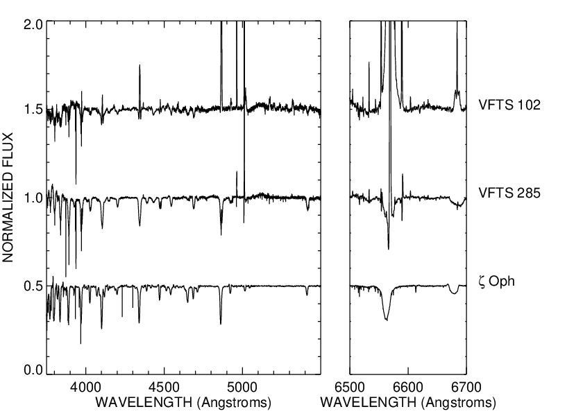
The X-shooter instrument was designed to record the spectra of a wide variety of astronomical objects, ranging from nearby faint point sources to bright extragalactic sources (Vernet et al. 2011). The observations for VFTS 102 were acquired under program 092.D-0108(A) (Przybilla), and additional spectra were obtained for both VFTS 102 and VFTS 285 under program 098.D-0375(A) (Gies). The X-shooter instrument records spectra in three arms corresponding to increasing wavelength bands labelled as UVB, VIS, and NIR (see Table 1). Collectively, these spectra cover a range from 3350 to 20800 Å. The spectra were reduced by the standard pipeline, normalized to unity at the continuum, and then co-added with weighting factors determined by the ratio.
The GIRAFFE spectrograph is a medium-to-high resolution spectrograph that was designed to record the optical spectra of high spatial density galactic and extragalactic objects (Pasquini et al. 2002). Spectral observations for both VFTS 102 and VFTS 285 were obtained as part of the VLT-FLAMES Tarantula Survey of massive stars in the 30 Doradus region in the LMC under programs 182.D-0222(A), (B), and (C). The observations were made using the Medusa fibers on the GIRAFFE spectrograph, which allow for up to 132 objects to be observed at once. The fibers have an entrance aperture equal to arcsec on the sky. The spectra utilized in this work cover a range from 3958 to 6820 Å and are labelled as UV, VIS, and NIR (corresponding to different bands than those with similar names for X-shooter; see Table 1). The reduced spectra were collected from the ESO Science Archive11 1 http://archive.eso.org/wdb/wdb/adp/phase3_spectral/form?phase3_collection=GIRAFFE_MEDUSA, rectified to unity at the continuum, and co-added to form one high ratio spectrum. In the final step, the X-shooter and GIRAFFE spectra were co-added where possible on a uniform grid for optimum . These coadded spectra were the focus of this study, and samples of the line profiles are presented in Figures 10 and 11 below. We did not reduce the effective resolving power of the X-shooter spectra to match that of the GIRAFFE spectra because the rotational broadening of the stellar features far exceeds that of the instrumental broadening, and as a result the line profiles appeared identical in both the X-shooter and GIRAFFE average spectra.
ESPaDOnS is a high resolution spectrograph and spectropolarimeter that was designed to record the optical spectrum with a resolving power of (Donati 2003). The ESPaDOnS spectra of Oph were obtained from the archive at the PolarBase website22 2 http://polarbase.irap.omp.eu/ (Petit et al. 2014) as a part of the Magnetism in Massive Stars (MiMeS) survey that collected data from 2005 to 2013 for 560 O- and B-type stars (Wade et al. 2015; Wade et al. 2016). The reduced spectra were rectified, and co-added on a uniform wavelength grid.
II.3 Spectral Energy Distributions
The rotation code described in §4 calculates both the line profiles and the absolute monochromatic flux in the nearby continuum regions. The absolute flux predictions taken together with the distance and interstellar extinction can be compared to the observed spectral energy distribution (SED) to determine the stellar radius. Figures 3, 4, and 5 show the observed SEDs for Oph, VFTS 102, and VFTS 285, respectively, together with the model estimates for 16 wavelengths (§4). The observed ultraviolet fluxes for comparison with the models were collected at the two FUV wavelengths from archival, high dispersion IUE spectra for Oph and from the HST/COS spectra for VFTS 102 and VFTS 285. The figures show instead low resolving power ( UV spectra from low dispersion IUE spectra for Oph and rebinned versions of the HST/COS spectra for VFTS 102 and VFTS 285. The optical fluxes of Oph are from the spectrophotometry of Burnashev 1985, and those for VFTS 102 and VFTS 285 are collected from various sources of broad-band photometry including VFTS (Evans et al. 2011), HTTP (Sabbi et al. 2016), SkyMapper (Wolf et al. 2018), and Gaia EDR3 (Gaia Collaboration et al. 2016; Gaia Collaboration et al. 2021). The infrared fluxes are collected from SAGE (Meixner et al. 2006), 2MASS (Skrutskie et al. 2006), and WISE (Wright et al. 2010).
Figures 3, 4, and 5 also show simple flux models for non-rotating stars from the TLUSTY grid (Lanz & Hubeny 2003) for the average temperature, gravity, abundance, distance, and extinction described in §4. These model spectra have a low resolving power similar to the observed broad-band fluxes, and they serve to show the general SED trends with wavelength. The SED of VFTS 102 displays an infrared excess from its circumstellar disk, and Figure 4 shows both the stellar component (dotted line) and combined stellar plus disk flux (solid line) for a simple power law expression for the disk flux (see §4.2). We will adopt wavelength-interpolated estimates of the optical monochromatic fluxes below (§4) directly from the observed values for the cases of Oph and VFTS 285, and from the star plus disk model fit for the case of VFTS 102.
III Radial Velocities of VFTS 102 and VFTS 285
The absorption lines in the spectra of both targets are extremely broad and shallow. Consequently, we need the best ratio possible in order to examine their rotationally broadened profiles. This can be accomplished for the ground-based, optical spectra through co-addition of the individual spectra. However, we need to first check for any evidence of radial velocity variability to insure that the spectra are properly wavelength registered before co-addition and to explore the possibility that these stars are spectroscopic binaries with faint companions (the possible remnant donors of past mass transfer). We describe below measurements of both the absorption and emission line features. Our results are summarized in Table 2 (VFTS 102) and Table 3 (VFTS 285).
There are two main methods that we use to make our measurements, the line bisector method for emission lines and the cross-correlation method for absorption lines. The bisector method is useful for the spectra of VFTS 102 which displays numerous emission lines formed in its circumstellar disk and in the surrounding nebula and SN remnant (known variously as 30 Dor B, Chu et al. 1992; N157B, Chen et al. 2006; and B0538-691, Micelotta et al. 2009). The bisector method determines the line center position by a Gaussian sampling of the line wings (Shafter et al. 1986). This has the advantage of measuring emission wings from the disk while ignoring the nebular emission that appears in the line core. We form a template using two oppositely signed Gaussians at offset positions from line center, and then the cross-correlation function (CCF) is made using this template and the emission line feature. The zero crossing of the resulting CCF yields the velocity corresponding to the wing bisector position. The wings of emission features form in the circumstellar disk close in to the star where the rotating disk has the highest Keplerian orbital motion. Since the disk is assumed to be centered on and tied to the star, by measuring the disk’s radial velocity we are also measuring the star’s radial velocity. In general we set the offset positions of the sampling Gaussians at velocities where the emission declines to of the peak value. However, if the feature has extraneous emission or absorption in the center due to residual problems from nebular sky subtraction or disk emission, we lower this threshold to around of the peak value in order to avoid the central region.
The second method was applied to the broad absorption lines in the spectra of both stars. We generated a model spectrum which was rotationally broadened to a projected rotational velocity of km s-1 using the TLUSTY/SYNSPEC model flux spectra from the OSTAR2003 grid of Lanz & Hubeny 2003. We then formed the CCF of the observed and model spectra over a wavelength range encompassing specific absorption lines. The exact regions that were used were limited to only the line profiles and did not include the continuum between features. The peak position of the CCF yielded an estimate of radial velocity.
The results for VFTS 102 appear in Table 2 which lists the heliocentric Julian date of mid-exposure, the spectrograph of origin, and radial velocities from the emission and absorption lines. The radial velocity measurements for the X-shooter spectra are averages from the emission features (column 3) of H, H, H, H I , and He I and from the absorption features (column 4) of H and He II . H consists of a broadened absorption feature with a double-peaked emission line in the center. Despite the central emission, we were able to measure the wings of the absorption line, so this radial velocity is included among the absorption line average.
We attempted to measure the radial velocities of the absorption lines reported by Dufton et al. 2011, which consist of He I and He II . However, we found that all but He II were too broad and shallow for reliable measurements in individual spectra. Dufton et al. 2011 used co-added spectra to enable their measurements.
The measurements of the GIRAFFE spectra include the emission features H, H, and H. Several of the GIRAFFE spectra have very low making the measurements difficult, and these are excluded from consideration. All of the emission line measurements were made using the line bisector method. The only absorption line measured was He II . In this case, we first cross-correlated the observed He II profile with a broadened model profile. We then measured the radial velocity using the line bisector on the CCF. This combination of methods allowed us to obtain a measurement from the He II feature despite its extremely shallow profile. The measurement from the HST/COS spectrum was aquired by cross-correlating the observed spectrum with a rotationally broadened model spectrum. We used a short wavelength region that includes N IV , C III (plus a blend of six other features), and Si III in addition to a mid-range region that includes Fe V and Si IV . The result is listed in column 4 of Table 2.
The final rows of Table 2 list the error weighted averages of all the measurements made from the X-shooter and GIRAFFE spectra. The uncertainties are the standard deviations of the individual measurements. There is satisfactory agreement between the absorption and emission line velocities, and this confirms that we are indeed measuring the radial velocity of the star itself through measurements of the disk gas emission. Additional verification comes from detailed fits made of the absorption lines presented in Section 5.2 below. Each model line was shifted in wavelength space until it matched the observed profile. This yields a radial velocity for each absorption line in the mean spectrum, and the average for the nine lines used in the analysis yields a radial velocity of (standard deviation) km s-1, in agreement with the results presented in Table 2. Furthermore, there is reasonable consistency in the results from X-shooter, GIRAFFE, and HST/COS. The weighted mean of the averages from both emission and absorption lines and all three instruments for VFTS 102 is km s-1.
The velocity results from the absorption lines in the spectra of VFTS 285 are given in Table 3. The radial velocities for the X-shooter spectra were obtained by cross-correlating a series of features with a rotationally broadened model. The features include H, H, H, and He II . The GIRAFFE measurements were obtained from cross-correlation functions based upon H, H, He I and He II . The measurement obtained for the HST/COS spectrum was obtained from the cross-correlation function of a short wavelength region (including C III and Si III ) and a mid-wavelength region (Fe V ). The bottom rows of Table 3 show that there is good agreement between the averages from X-shooter and GIRAFFE. The mean of the X-shooter, GIRAFFE, and HST/COS results is km s-1.
=0.1mm
| Heliocentric | Spectrograph | (emission) | (absorption) |
|---|---|---|---|
| Julian Date | Name | (km s-1) | (km s-1) |
| 2454822.754 | GIRAFFE | 265 18 | |
| 2454822.797 | GIRAFFE | 268 10 | |
| 2454822.840 | GIRAFFE | 266 11 | |
| 2454825.740 | GIRAFFE | 269 15 | 252 27 |
| 2454825.783 | GIRAFFE | 268 16 | 235 11 |
| 2454825.826 | GIRAFFE | 267 18 | 248 4 |
| 2454858.720 | GIRAFFE | 266 8 | |
| 2454889.552 | GIRAFFE | 262 9 | |
| 2455114.772 | GIRAFFE | 199 30 | |
| 2456605.711 | X-shooter | 271 2 | 268 11 |
| 2456606.726 | X-shooter | 274 2 | 267 10 |
| 2457299.761 | GIRAFFE | 274 18 | |
| 2457335.798 | GIRAFFE | 264 10 | |
| 2457339.714 | GIRAFFE | 261 12 | |
| 2457339.796 | GIRAFFE | 263 17 | |
| 2457366.740 | GIRAFFE | 260 16 | |
| 2457394.668 | GIRAFFE | 266 9 | |
| 2457398.739 | GIRAFFE | 262 12 | |
| 2457400.582 | GIRAFFE | 251 40 | |
| 2457402.618 | GIRAFFE | 265 19 | |
| 2457415.563 | GIRAFFE | 262 12 | |
| 2457416.575 | GIRAFFE | 261 14 | |
| 2457417.579 | GIRAFFE | 271 11 | |
| 2457418.628 | GIRAFFE | 273 14 | |
| 2457420.638 | GIRAFFE | 268 11 | |
| 2457423.615 | GIRAFFE | 266 16 | |
| 2457427.623 | GIRAFFE | 269 9 | |
| 2457432.533 | GIRAFFE | 280 13 | |
| 2457622.882 | GIRAFFE | 267 14 | |
| 2457681.726 | GIRAFFE | 272 9 | |
| 2457692.759 | GIRAFFE | 267 13 | |
| 2457698.764 | GIRAFFE | 258 10 | |
| 2457726.726 | GIRAFFE | 264 12 | |
| 2457755.380 | HST/COS | 223 15 | |
| 2457797.584 | X-shooter | 267 2 | 269 11 |
| 2457819.533 | X-shooter | 268 2 | 257 11 |
| Average | X-shooter | 270 3 | 265 6 |
| Average | GIRAFFE | 266 13 | 247 9 |
| Heliocentric | Spectrograph | (absorption) |
|---|---|---|
| Julian Date | Name | (km s-1) |
| 2454794.686 | GIRAFFE | 248 4 |
| 2454794.730 | GIRAFFE | 248 4 |
| 2454794.828 | GIRAFFE | 270 4 |
| 2454798.803 | GIRAFFE | 276 5 |
| 2454836.645 | GIRAFFE | 245 4 |
| 2454836.691 | GIRAFFE | 245 4 |
| 2454867.558 | GIRAFFE | 251 4 |
| 2457299.761 | GIRAFFE | 232 4 |
| 2457332.749 | GIRAFFE | 261 4 |
| 2457335.798 | GIRAFFE | 251 4 |
| 2457339.714 | GIRAFFE | 258 4 |
| 2457339.796 | GIRAFFE | 255 4 |
| 2457366.740 | GIRAFFE | 238 4 |
| 2457379.567 | GIRAFFE | 269 4 |
| 2457394.668 | GIRAFFE | 243 4 |
| 2457398.739 | GIRAFFE | 249 4 |
| 2457400.582 | GIRAFFE | 268 5 |
| 2457402.618 | GIRAFFE | 229 12 |
| 2457415.563 | GIRAFFE | 254 4 |
| 2457416.575 | GIRAFFE | 268 4 |
| 2457417.579 | GIRAFFE | 268 4 |
| 2457418.628 | GIRAFFE | 258 4 |
| 2457420.638 | GIRAFFE | 234 4 |
| 2457421.711 | GIRAFFE | 270 3 |
| 2457423.615 | GIRAFFE | 253 4 |
| 2457427.623 | GIRAFFE | 267 4 |
| 2457432.533 | GIRAFFE | 254 4 |
| 2457488.626 | HST/COS | 252 17 |
| 2457622.882 | GIRAFFE | 247 5 |
| 2457651.777 | GIRAFFE | 233 6 |
| 2457681.726 | GIRAFFE | 263 4 |
| 2457692.759 | GIRAFFE | 268 4 |
| 2457698.764 | GIRAFFE | 254 4 |
| 2457724.723 | GIRAFFE | 243 9 |
| 2457726.726 | GIRAFFE | 263 4 |
| 2457765.726 | X-shooter | 240 3 |
| 2457766.733 | X-shooter | 241 3 |
| 2457775.634 | X-shooter | 256 5 |
| 2457787.536 | X-shooter | 243 4 |
| 2457790.533 | X-shooter | 249 4 |
| 2457790.570 | X-shooter | 253 3 |
| Average | X-shooter | 247 7 |
| Average | GIRAFFE | 259 13 |
The standard deviation between observations (external error) is approximately the same as the mean of the individual error estimates (internal error) for both stars, so they appear to be radial velocity constant. Thus, we can reasonably perform a simple co-addition of the spectra to improve the without needing to consider shifting individual spectra to account for any binary orbital motion. The final mean velocities are and km s-1 for VFTS 102 and VFTS 285, respectively, which are the error weighted mean and uncertainty from the sample averages at the bottom of Tables 2 and 3. These radial velocities are comparable to the average for the single, B-type stars in the 30 Dor region, km s-1, found by Evans et al. 2015. In both cases, our results are slightly higher than found in earlier work: km s-1 (Dufton et al. 2011) and km s-1 (Sana et al. 2013) for VFTS 102 and km s-1 (Sana et al. 2013) for VFTS 285. However, given the difficulty of measuring such broad and shallow absorption lines and differences in our methods, we doubt that the resulting differences in velocity are significant.
IV Spectral Synthesis Models
Our primary goal is to compare models of the flux emitted by very rapidly rotating stars with observed spectral line profiles and the associated spectral energy distribution. Each model is based on parameters for its equatorial rotational velocity, physical parameters, and axial orientation to our line of sight. Fits of the model spectra to the observed spectra help inform final estimates of all these parameters. In this section, we describe the elements of the model and the parameter fitting methods. The results of the model fitting are discussed in §5.
IV.1 Method
We utilize a numerical code that simulates the distorted shape and latitude-dependent photospheric properties of a rapidly rotating star that is viewed at an inclination angle between the axis of rotation and the line of sight. The spectral line synthesis code is written in IDL, and the original version was presented by Huang & Gies 2006. The shape of the star is defined by Roche geometry which assumes that most of the mass is concentrated towards the stellar core. The stellar photosphere is represented by a grid of 40,000 surface elements with approximately equal area that are distributed in co-latitude and azimuth . An integration is made of the flux from each surface element by first calculating the angle between the surface normal and the line of sight in order to determine if the element is situated on the visible hemisphere of the star. For each element, the code determines a local effective temperature (dependent on the gravity darkening model; §4.4), effective gravity (gravitational plus centrifugal), area of the surface element projected in the sky (dependent on = cosine of the angle between the surface normal and line of sight), and the rotational radial velocity (assuming solid body rotation). These parameters are used to interpolate in a pre-computed grid of spectral specific intensities as a function of wavelength, , , and associated with an assumed chemical abundance. The product of the projected area and the specific intensity yields the flux increment from the element, and the sum of all such increments gives the total flux to be compared with the observations. The outputs are a wavelength dependent line profile and a monochromatic flux estimate for the immediate vicinity of a particular spectral feature or line blend. This type of spectrum synthesis is common among many past investigations of rotational shape and spectral line broadening (Collins 1963; Stoeckley 1968; Howarth & Smith 2001; Townsend et al. 2004; Aufdenberg et al. 2006; Abdul-Masih et al. 2020).
The model parameters are listed in Table 4 together with the derived values for the three target stars of this study. Column 2 identifies those parameters that are fit (F), set in advance (S), and derived in the model from the previous parameters (D). The set of fitting parameters includes the projected rotational velocity , rotational axis inclination , polar radius , stellar mass , polar effective temperature , He abundance by number relative to H, and interstellar reddening . The set parameters were determined by independent constraints, and they include the adopted gravity darkening law (§4.4), distance , and ratio of total-to-selective extinction (§4.2). The remaining derived parameters describe the physical characteristics of the star and the goodness-of-fit of the model. The derived rotation parameters are the equatorial rotational velocity , the critical velocity in the Roche model (where the equatorial radius is the polar radius and centrifugal acceleration balances gravity at the equator), and the ratio of the angular velocity to the critical angular velocity (Rieutord 2016). The other physical parameters for the star include the equatorial radius , the logarithm of the effective gravity at the pole , at the equator , averaged over the visible hemisphere (avg), the effective temperature at the equator , and the flux-weighted average temperature (avg). We also calculate the area-integrated average temperature (all) and logarithm of the total luminosity by integrating over the entire surface. Those parameters listed with solar units were obtained by adopting the IAU recommended nominal values for the Sun (Prša et al. 2016).
| Parameter | KindaaD = derived from model; F = fit; S = set. | Oph | OphbbFrom Howarth & Smith 2001. | VFTS 102 | VFTS 285 | VFTS 285 |
|---|---|---|---|---|---|---|
| Gravity darkening | S | -model | von Zeipel | -model | -model | von Zeipel |
| (km s-1) | F | 400 | ||||
| (degrees) | F | |||||
| (km s-1) | D | 413 | 425 | 649 | 648 | 726 |
| (km s-1) | D | 508 | 652 | 796 | 795 | |
| D | 0.95 | 1.00 | 0.95 | 0.99 | ||
| () | F | 7.5 | ||||
| () | D | 8.11 | 8.08 | 7.16 | 7.65 | |
| () | F | 20.0 | ||||
| (dex cgs) | D | 3.94 | 4.23 | 4.39 | 4.39 | |
| (dex cgs) | D | 3.35 | 3.58 | 2.26 | 3.81 | 3.47 |
| (avg) (dex cgs) | D | 3.62 | 3.64 | 4.05 | 4.01 | |
| (kK) | F | |||||
| (kK) | D | 28.3 | 30.7 | 23.2 | 31.6 | 25.3 |
| (avg) (kK) | D | 31.4 | 32.9 | 34.9 | 35.0 | |
| (all) (kK) | D | 31.4 | 34.3 | 33.3 | 35.0 | 33.3 |
| D | 4.67 | 4.96 | 4.75 | 4.76 | 4.71 | |
| F | ||||||
| (kpc) | S | 0.14 | ||||
| S | 2.76 | 2.76 | 2.76 | |||
| (mag) | F | |||||
| [line] | D | 16.5 | 1.7 | 4.1 | 4.1 | |
| () | D | 0.042 | 0.127 | 0.056 | 0.057 |
There are several simplifications in the model that are justifiable assumptions. The shape of a star is subject to differential rotation, but detailed calculations suggest that differential rotation is modest in rapidly rotating massive stars (varying by only a few percent with colatitude; Espinosa Lara & Rieutord 2013). Consequently we expect that our neglect of differential rotation and the use of the Roche model for the stellar surface are good approximations (Zahn et al. 2010; Rieutord 2016). The spectral specific intensity calculations are based upon plane-parallel stellar atmospheres (§4.3), so effects due to extended atmospheres and stellar winds are not treated. However, we expect any such effects to be minimal in the case of the three targets discussed here. We showed in an earlier paper (Shepard et al. 2020) that wind features are present in some spectral lines in the ultraviolet, and we discuss the influence of the circumstellar disk of VFTS 102 below (§4.2). Finally, we are neglecting any processes related to macroturbulence in this analysis. Simón-Díaz & Herrero 2007 used a Fourier transform method to analyze the broadened spectral line profiles of O-type stars to extract both the projected rotational velocity and the macroturbulent velocity, and they argue that macroturbulence generally becomes a significant contributor to line broadening among the more luminous supergiant stars (Simón-Díaz & Herrero 2014). The net line broadening varies approximately as the quadratic sum of the rotational and macroturbulent velocities, and because the rotational component is so dominant in the stars discussed here, we can safely neglect any macroturbulent broadening terms.
IV.2 Integrated Flux
The model calculates the integrated monochromatic flux produced by the star, and this can be compared to the observed flux to help estimate the stellar radius. For a spherical star, the ratio of the observed to emitted flux is
where is the angular diameter and is the wavelength-dependent extinction. Thus, this ratio becomes an important criterion to establish the stellar polar radius of a rotating star once the distance and extinction are known. Here we fix the known distances of the targets and solve for a reddening that sets the amount of interstellar extinction according to an adopted value of the ratio of total-to-selective extinction .
Our adopted distances are listed in Table 4. The distance of Oph is taken from the parallax measurement from Gaia EDR3 (Bailer-Jones et al. 2021), and this value is in good agreement with other independent estimates (Gordon et al. 2018). The distance of VFTS 102 and VFTS 285 is set to the accurate LMC distance from Pietrzyński et al. 2019 based upon eclipsing binaries and other standard candles in the LMC.
The wavelength dependent extinction curve is taken from the model described by Fitzpatrick 1999 that is determined from the reddening and ratio of total-to-selective extinction . We solve for by comparing the observed and model SED using an adopted value for (Table 4). This is set to the result from Zuo et al. 2021 for Oph. Unfortunately, there are no published results on for the two LMC targets. We adopted the value of for the nearby LMC2 supershell region determined by Gordon et al. 2003 (and we used their special extinction prescription for VFTS 102 and VFTS 285), although we caution that the actual value may vary considerably among the stars of the 30 Dor region. For example, both Maíz Apellániz et al. 2014 and De Marchi & Panagia 2019 find a larger value of the ratio, .
Special care is required in the flux analysis of VFTS 102, because this star has an extensive circumstellar disk that also contributes to the observed flux. The SED of VFTS 102 (Fig. 4) shows a strong infrared excess that is a common signature of circumstellar disks around Be stars (Vieira et al. 2015; Klement et al. 2019). The disk emission is often represented approximately as a power law (Waters 1986),
where is the observed star plus disk flux, is the stellar flux rescaled by distance, is wavelength in reference to a standard wavelength m, is the extinction, and and are the power law parameters describing the infrared excess. A simple fit of the SED using a TLUSTY model for the stellar flux was obtained with and , and is shown with the observed SED in Figure 4.
This disk flux excess in the spectrum of VFTS 102 has two important consequences: (1) the model stellar flux must be increased by the amount of the flux excess before comparison with the observed flux, and (2) the model line depths need to be reduced to account for the excess continuum flux (sometimes referred to as “line veiling”). We did this by calculating a line depth factor at the central wavelength of each line,
The model stellar fluxes were divided by to rescale them to the total star plus disk flux, and the continuum normalized line depths were multiplied by to account for the added disk continuum, i.e.,
where is the continuum normalized spectrum (§4.5). This approach corrects for the added continuum flux of the disk, but not for any stellar flux that may be obscured by the disk if seen edge on. The calculations necessary to account for disk obscuration are outside the scope of this paper, and we therefore leave this complication to future work.
IV.3 Specific Intensity Profiles
The core of the simulation is the radiative specific intensity that we derive from two TLUSTY grids of line-blanketed, non-LTE, model atmospheres, OSTAR2002 (Lanz & Hubeny 2003) and BSTAR2006 (Lanz & Hubeny 2007). High resolving power model spectra are calculated from these model atmospheres using the SYNSPEC radiative transfer code (Hubeny & Lanz 2017). These assume the solar abundance pattern from Grevesse & Sauval 1998 for Galactic “G” models (with a He abundance by number relative to H of ) that we use in the line synthesis for Oph. We adopt their LMC “L” models that have the same H and He abundance with all other elements reduced by half (Rolleston et al. 2002) for the analyses of VFTS 102 and VFTS 285. We found it necessary to explore models with greater than solar He abundance (§4.7), and this was done by a numerical up-scaling of the He to H number ratio by , , and the solar value with the SYNSPEC code. We caution that this is an approximation that is not fully self-consistent with the abundances assumed in the TLUSTY atmospheres.
The BSTAR2006 grid covers the temperature range from 15 to 30 kK for an assumed microturbulent velocity of 2 km s-1, while the OSTAR2003 grid ranges from 27.7 to 55 kK using a microturbulent velocity of 10 km s-1. In order to create a smooth transition between these differing cases, we formed a temperature grid with a step size of 1 kK (like that in the BSTAR2006 grid), and then interpolated in the temperature overlap region scaling by , , and between the BSTAR2006/OSTAR2003 grids at 28, 29, and 30 kK, respectively.
For each spectral region, the SYNSPEC results were transformed to a common and equally spaced wavelength grid to create a specific intensity matrix, for 10 equal steps in , the cosine of the angle between the normal and line of sight, from 0.1 to 1.0, 41 steps in from 15 to 55 kK, and 12 steps in from 2.0 to 4.75. These matrices were calculated for two regions in the far-ultraviolet and 14 regions in the optical spectrum for comparison with the observed spectra (§5). We show an example of these specific intensity profiles in Figure 6. These show that the central depths of strong lines are almost the same at all angles (formed high in the atmosphere where the temperature and line source function are approximately constant) while the continuum levels decline from to 0.1 (limb darkening associated with the drop in temperature and source function higher in the atmosphere). Thus, in a continuum normalized representation, the spectral line depths look relatively weaker at the limb () compared to the center of the stellar disk (). This is a reminder that the observed rotational broadening is not strictly a convolution of a fixed depth photospheric profile and a rotational broadening function.

Our analysis of the spectral lines is based upon this framework of specific intensities from the published TLUSTY grids, so the results are dependent on the approximations in the code in addition to those described above. For example, TLUSTY includes the turbulent pressure associated with microturbulence as a component of the total pressure. Thus, the pressure treatment is different between the BSTAR2006 and OSTAR2003 grids because of the different assumed values of microturbulence (2 and 10 km s-1, respectively), and this might influence the model Stark broadening of the H Balmer lines (important in the derivation of stellar mass; Section 4.6). However, the BSTAR2006 grid does include the larger 10 km s-1 microturbulence value in a subset of models appropriate for lower gravity giants and supergiants. A comparison of model H lines for the same parameters but with microturbulent velocities of 2 and 10 km s-1 shows only very small differences in the profiles. Thus, the hybrid treatment of microturbulence in this application should have no significant impact on our results.
IV.4 Gravity Darkening
von Zeipel 1924 found that the local energy radiated (and hence the local temperature) of a rotating star varies as , so that the higher gravity pole is hotter than the equator. However, this can only be strictly correct in cases where the gas is barotropic (pressure dependent on density only), which is generally not the case for stars (Rieutord 2016). The full solution to the problem requires consideration of the interior state and motions (ESTER code; Espinosa Lara & Rieutord 2013). Fortunately Espinosa Lara & Rieutord 2011 found an analytical representation of the surface temperature variation with colatitude that matches that from the detailed models quite well. We used this -model in our code by solving equations 18 and 23 in the development presented by Rieutord 2016 to determine the ratio of .
Generally we adopt the -model for our models, however, we show an example of how the line profiles differ between the predictions of the von Zeipel law and the -model. Figure 7 shows the results for a model star with , , kK, km s-1, and km s-1, i.e., a case close to critical rotation. The images in the first column show the surface brightness (specific intensity) in the far-ultraviolet (1181 Å) where the contrast between the pole and equator is especially striking. The top image shows the limb darkened disk for the corresponding non-rotating model, while the lower three images show the same stellar model at near critical rotation described by the -model with inclination angles of , , and . The next columns illustrate the appearance of several surface-integrated flux profiles for these orientations and the two gravity darkening laws considered. The top row shows the non-rotating case for the spectrum in the vicinity of C III , He I , and He II . The next three rows give the rotationally broadened model profiles plotted as a function of Doppler shift relative to . If plotted versus actual Doppler shift the profiles would appear narrower at lower inclination (, 562, and 458 km s-1 for rows 2,3, and 4, respectively) due to the inclination shift from equator-on, where the extreme rotation is best observed, to pole-on, which shows no rotational broadening. However, by plotting the profiles relative to , it is easier to discern overall changes in the shape of the line profile with inclination and between the predictions for the -model (solid lines) and von Zeipel law (dotted lines) for gravity darkening.

These models help to demonstrate how the differences between the gravity laws manifest in line profiles. The -model predicts a pole to equator temperature variation that is less extreme than that from the von Zeipel prescription. This difference shows up best in the He II profiles for (row 2, column 4). In the von Zeipel case, the darker equator is more extensive and hotter pole more limited in colatitude, and because the He II line is preferentially formed in hotter environments, it appears weaker in the von Zeipel case where hot conditions are confined to a smaller area. The opposite is true of the other lines that grow in strength at relatively cooler temperatures.
A comparison of the relative changes in line shape and strength with inclination angle shows that some lines change significantly (He II) while others are approximately constant (C III). This demonstrates that an analysis of the rotational broadening among a sample of different line species can potentially help to constrain the value of the rotational inclination.
IV.5 Transformation to the Observer’s Frame
The derived model spectrum is created in units of physical flux in the rest wavelength frame of the star, and there are several steps required in order to compare the model directly with the observed line profile. The first step is to shift the spectrum to the observed Doppler shift of the star. Initially we assumed a radial velocity of km s-1 for Oph (Reid et al. 1993), however we made a number of small revisions to this estimate for the different lines in the sample. We adopted the mean of the radial velocities of VFTS 102 and VFTS 285, but again we introduced small changes ( km s-1) on a line-by-line basis in order to align the model and observed line profiles. The model profiles were then transformed to the observed wavelength grid by an integration scheme.
The spectra were re-normalized to a unit continuum by selecting wavelength regions immediately to the blue and red of the main absorption feature, where we formed the ratio of observed-to-model fluxes in these regions. The model spectrum was then multiplied by a linear fit of the flux ratios in the rectification regions, so that the local continua of the observed and model spectra are in agreement. The resulting model spectrum was then convolved with a Gaussian function to account for the minor amount of instrumental broadening associated with each spectrograph. The models of spectra for VFTS 102 were subject to a small reduction in line depth to account for the wavelength-dependent contribution of extra continuum flux from the circumstellar disk (§4.2). Finally the calculated portion of the model spectrum was inserted into an otherwise flat continuum spectrum outside of the wavelength range in the simulation, and these boundaries appear in some of the spectral plots below where there appears to be a sudden jump to unity.
IV.6 Parameter Fits
Our goal is to optimize the seven fitting parameters given in Table 4 in order to best match the observed and model fluxes and rectified line profiles. We found that we could converge to a unique solution through a guided grid search method that relies primarily on the continuum fluxes to set and , and then uses fits of the line profiles to help determine , , , and . The final parameter is the He abundance which we discuss separately in the next subsection.
The procedure begins using assumed values for the parameters that are reasonably well known at the outset: , , , and . The first step is to compare the observed and model fluxes that span the full ultraviolet to optical range (including the circumstellar disk flux contribution in the case of VFTS 102). We perform preliminary model simulations and check if there are any systematic trends in the observed-to-model flux ratio as a function of wavelength. If so, then the reddening parameter is revised in order to find consistent observed-to-model flux ratios across the spectrum. Next, we consider the mean value of the observed-to-model flux ratio, and we revise the polar radius in order to make this ratio unity for the given values of distance and interstellar extinction (set through the derived and fixed values).
The procedure next considers the fits of the spectral line profiles. A goodness-of-fit estimate is found by comparing the observed and model line profiles over a limited wavelength range that spans the full absorption profile while excluding any problem regions that are marred by background nebular or disk emission. This is particularly important in the case of VFTS 102, where fits of the H and He I lines were restricted to the extreme line wings to avoid emission components in the central parts of these profiles. The scatter between the observed and model profiles is compared to that in nearby continuum regions to find a reduced chi-squared statistic for each spectral feature. The code also measures the ratio of (Observed - Calculated) / Observed equivalent width to determine the sense of remaining discrepancies in the model, and these are used to estimate the He abundance (§4.7).
The observed and model line comparison begins with the H-Balmer lines that are sensitive to both temperature and gravity (through Stark broadening) in the O- and B-type stars. With the polar temperature and radius set at this stage, the gravity dimension is explored through the calculation of the Balmer lines for a test grid of model masses. For each test value of mass, we create model Balmer lines from an integration of the surface with the local gravity set for each surface element based upon its radial distance from the center of the star and its rotational velocity, and then the corresponding specific intensity profile (with the associated Stark broadening) is derived from the pre-computed set (§4.3). Then we compare the model and observed flux profiles to determine the goodness-of-fit for each Balmer line. A spline fit is made of the variation of the mean as a function of assumed mass, and the minimum of this fit yields the estimate of mass .
The basic procedure outlined above is repeated over a grid of test values for polar temperature , and the variation with assumed of the mean derived from all the lines in the sample is used to find the best fit polar temperature. The final step is to conduct this complete analysis over a grid of assumed inclination and projected rotational velocity , determine the global minimum of the mean , and find estimates for and .
We found that there were significant mismatches between the observed and model profiles for certain line profiles that occurred in the analysis of all three target stars. These are systematic problems related to incomplete lists of possible line blends with other features, non-standard abundances, and/or problems with the physical properties assigned to the atomic transitions in TLUSTY/SYNSPEC. After some experimentation, we limited the line sample to a set that gave mutually consistent results, therefore any systematic errors that remain in the analysis are treated consistently for all three stars. The line set adopted for the parameter estimation includes H , H , H , He I , and He II . We show in §5 the fits for these nine features and for the remaining seven excluded line profiles.
IV.7 Helium Abundance
We noticed at the outset of the analysis that the He line model profiles calculated using specific intensity matrices based upon the solar He abundance were often much weaker than the observed profiles. Consequently we computed additional model specific intensity matrices using SYNSPEC for assumed He abundances of , , and the adopted solar value. The same parameter fitting procedure was conducted for these different He abundances and the He line trends were examined in each case to determine how the models predicted He line strengths that were systematically too weak and too strong.
We show an example of the trends in Figure 8 for the case of Oph. The corresponding trends found for VFTS 102 and VFTS 285 are qualitatively similar. Figure 8 shows the fractional differences in (Observed - Calculated) / Observed line equivalent width as function of assumed polar temperature for three He I and three He II lines. The He II equivalent width ratios show a net decline from underestimating the strength to overestimating the strength with increasing . The He I equivalent width ratio shows the opposite trend as expected, while the He I ratios are approximately constant. We suspect that the latter two features are actually line blends that change with temperature in differing ways so that the composite profile is relatively constant (for example, the blend of He I and He II ). The large plus sign near the center marks the average position of all the He I and He II trend crossings. This occurs at for the solar model (left panel; He too weak) and at for the solar model (right panel; He too strong). Thus, the best match of the He line strengths occurs for an intermediate He abundance between these cases.
We made similar plots for all four test cases of He abundance , and we used a spline fit of to find the zero-crossing position that corresponds to the best fit of the helium abundance based upon these six He lines. The results are listed with the other parameters in Table 4 with uncertainties based upon the scatter in the He I and He II intersection points in these plots.
IV.8 Parameter Uncertainties
The predominant source of uncertainty in the parameter estimations comes from the spread in derived parameter values for fits of the individual lines in the default set of three H, three He I, and three He II features. These are systematic errors related to the model itself, so in most cases we have estimated the parameter uncertainties from the line-to-line standard deviation of the results found using the individual line fits. There are two other sources of significant uncertainty that must also be considered. The fractional uncertainty in distance is largest for the case of Oph (), therefore this is the most important factor in assessing the uncertainty in polar radius which is linearly dependent on the assumed distance. The other key element in the uncertainty is the interstellar extinction that depends on the assumed value of the ratio of total-to-selective extinction . The reddening is modest for Oph and VFTS 285, so the underlying uncertainty in has only a small affect on the results. However, the reddening of VFTS 102 is much larger, so uncertainties in are important. We tested the sensitivity of the results by making simple SED fits (like those in Fig. 4) for both the adopted value of and the nominal value of , and we found that the derived angular diameter increased by using the latter value. The polar radius varies directly with angular size, so we included this factor in the final uncertainty estimate for for VFTS 102.
The bottom two rows of Table 4 list the statistics associated with the fits. The reduced chi-square is the average of the individual chi-square measurements for all the lines used in the sample. It can be somewhat misleading given the complicated and often deceiving nature of extreme rotational broadening. For example, is the smallest for fits of the lines of VFTS 102, but this is mainly the result of extremely shallow lines that have a depth not much larger than the scatter in the continuum. The final row reports the standard deviation of the observed to model flux ratio for all 16 spectral regions from the FUV to the optical, and it provides a sense of the success of the flux fits (worse in the case of VFTS 102 where complications exist due to the flux of the circumstellar disk). The fits associated with the parameter estimates in Table 4 are discussed in the next section.
V Spectrum Synthesis Fitting Results
V.1 Oph
Figure 9 shows the 16 spectral features that we modeled with the rotation code described in §4. The default set of nine lines used in the parameter fitting code (indicated by asterisks in the identifying labels) are generally well fit by the model, however discrepancies from the fit in other cases deserve some comment. The C III feature appears to show a significant blue-shift compared to the model, and we suspect that this transition is partially influenced by the stellar wind, appearing like a weak P Cygni feature (observed as a wind feature in the O-star binary UW CMa; Drechsel et al. 1981). The other ultraviolet feature is the Fe IV blend that appears to be slightly too weak in the model, perhaps due to the choice of microturbulence in the TLUSTY model or to uncertainties in the atomic oscillator strengths. The H , He I , and He II lines all appear to be consistently too deep in the model (including the C III line in the blue wing of the latter), so they were excluded from the parameter fit. The longer wavelength transitions of He I appear to show disk-like emission in their extreme wings (possibly also present in He I ), so they were also omitted from the fit. The spectrum of Oph does occasionally exhibit double-peaked emission like that of the disk emission observed in Be stars (Vogt & Penrod 1983), but no H emission is apparent in the Oph spectra used here.
Our motivation for including Oph in this study was to test our parameter fitting results with those obtained independently using a similar code by Howarth & Smith 2001. The two sets of results are compared in columns 2 and 3 of Table 4. There is good agreement in most of the derived parameters. The polar temperature derived by Howarth & Smith 2001 is slightly higher due to our use of fully line-blanketed model atmospheres that tend to assign lower than models based on H and He line opacities alone (Lanz & Hubeny 2003). The other difference is the use of the von Zeipel law for gravity darkening used by Howarth & Smith 2001. The equator to polar temperature contrast is larger in the von Zeipel description versus the -model for a given rotation rate, and we arrive at the same ratio of as derived by Howarth & Smith 2001 (who utilized the Von Zeipel law) by using a relatively larger angular velocity ratio when using the -model.
Our derived He abundance is the same within uncertainties as found by Howarth & Smith 2001, , confirming the apparent He enrichment in the atmosphere of Oph. Models that neglect the changes of the star’s shape and gravity darkening due to rotation tend to arrive at a lower He abundance: for example, from Herrero et al. 1992, from Villamariz & Herrero 2005, and from Cazorla et al. 2017. The fast projected rotational velocity we find is similar to that found in most other studies, with the exception of Simón-Díaz & Herrero 2014, who split the apparent broadening between rotation, km s-1, and macroturbulence, km s-1.
V.2 VFTS 102
Many of the spectral line features of VFTS 102 are altered in some way by the presence of a well-developed circumstellar disk. We discussed above in §4.2 how disk emission adds to the spectral energy distribution at longer wavelengths and how the disk continuum acts to make the spectral lines appear shallower. The other striking aspect is how the disk emission appears as a new profile component in the core of the H Balmer and He I lines as shown in Figure 10. For these cases, the observed and model profile goodness-of-fit statistic was calculated only for the line wing portions of the profile where no disk emission appears. This approach is successful in showing the presence of residual disk emission that is not obvious on first inspection (for example, the He I profile in Fig. 10). Making a fit of the line wings failed in the case of H because disk emission extends into the far wings, so this feature was omitted from the parameter fitting procedure. This leaves only fits of H and H for the determination of the mass through the apparent Stark (collisional) broadening. Tests showed that omission of H in fits of the spectra of Oph and VFTS 285 changed the derived mass by less than , therefore we doubt the omission of H has any significant impact on the final parameter solution for VFTS 102.
The derived average parameters in Table 4 all agree within uncertainties with those estimated in the discovery paper by Dufton et al. 2011 (see their Table 1). In particular, the estimate of projected rotational velocity km s-1 is the largest among all three stars, and the equatorial velocity is the same as the critical velocity within errors. Thus, VFTS 102 appears to be a star that has attained critical rotation. This extraordinary spin probably assists those mass loss processes that feed gas into the circumstellar disk, creating a vigorous decretion disk despite the disk gas ablation that occurs due to the harsh radiation field of the star (Kee et al. 2016).
V.3 VFTS 285
The rotational model parameter fits for VFTS 285 indicate that the star is the hottest and most massive of the three targets. The star’s true equatorial velocity is about the same as that of VFTS 102, however because the star is more massive, the critical velocity is higher, and therefore the star has a sub-critical spin, . The hotter temperature and slower spin relative to critical rotation are probably the reasons why no circumstellar disk is found for VFTS 285 (in contrast to the case of VFTS 102; §5.2). The average parameters given in column 5 of Table 4 agree within errors with those derived from Sabín-Sanjulián et al. 2017 that do not include rotational deformation in the model. The one exception is the He abundance that Sabín-Sanjulián et al. 2017 find to be only somewhat enhanced, compared to our result of (the largest He overabundance among the three stars). This same kind of difference was noted above between rotating and non-rotating physical model results for Oph (§5.1). In the non-rotating models He II line formation occurs over the entire visible hemisphere, while in the rotating models that include gravity darkening, He II line formation is more restricted to the hotter polar zones (because the He II lines weaken in the cooler equatorial zone). Consequently, in order to match the observed line strength, the rotating models compensate for the smaller area of formation by increasing the He abundance. The other difference in our work is the neglect of stellar winds in the TLUSTY models. The He II line that we use is sensitive to wind emission in more luminous stars (Walborn 1971), but in the case of VFTS 285, the model He II line appears to match the observed line as well as found for the other He II lines (Fig. 11).
The spectral line fits shown in Figure 11 are mostly satisfactory among the default set (marked by asterisks in the figure panels), except in the cores of some of the H Balmer and He I lines where sharp features remain from over- or under-subtraction of the nebular emission from the surrounding gas. These core regions were excluded from the goodness-of-fit measurements.
We decided to experiment with model fits of the spectral features of VFTS 285 by changing the gravity darkening prescription to the von Zeipel law in order to demonstrate how the choice of gravity darkening influences the solution. The resulting parameters using the von Zeipel law are shown in the final column of Table 4. We found that the model predicted He I and He II line profiles that were still too weak () compared to the observed profiles even with the largest assumed He overabundance, (§4.7). Thus, applying a rotational model using the von Zeipel law appears to lead to an over-estimate of He abundance in this case. Rather than extrapolate to even higher He abundances, we simply report the results of the fits in Table 4. The von Zeipel model is best fit with a star that is rotating somewhat closer to the critical rate with greater equatorial extension and a larger range in the polar to equatorial temperature.
VI Evolutionary Origins
VI.1 Single Star Models
Both VFTS 102 and VFTS 285 display exceptionally large rotational line broadening compared to other O-type stars in the VFTS sample (Ramírez-Agudelo et al. 2013). Here we consider what processes may have contributed to their extreme spins. The first possibility is that both are very young stars that attained their rapid spin due to accretion of their natal disks. Ekström et al. 2008 and Brott et al. 2011 calculated evolutionary tracks for stars born as rapid rotators, and in Figure 12 we show evolutionary tracks in the Hertzsprung-Russell Diagram (HRD) for three massive stars from Brott et al. 2011. These particular tracks were made assuming LMC abundances and initial equatorial velocities of km s-1. The track for the model shows the normal evolution to higher luminosity and cooler temperature as core H-burning concludes, but the tracks for and show evolution to higher temperatures. This behavior in massive, fast rotators is due to extensive mixing in the interior that replenishes the H core and dredges up the processed He into the envelope. Thus, mixing tends to homogenize the composition of the core and envelope.

We also plot in Figure 12 the derived estimates of (all) and from Table 4 for VFTS 102 and VFTS 285. Note that the estimates for the models of Brott et al. 2011 are based upon an average over the surface of the star assuming a von Zeipel gravity darkened flux, so they are not exactly comparable to our results for the -model (but the difference is small; see the two gravity darkening cases for VFTS 285 in Table 4). Furthermore, the model equatorial velocities are somewhat smaller than our estimates for the stars, so trends related to rotation might be even more extreme for evolutionary tracks at higher rotation speeds. The position of VFTS 102 is somewhat overluminous for its estimated mass () and is slightly cooler than predicted for the age of the nearby stars in the vicinity of the LH 99 OB association of 5.7 Myr (Schneider et al. 2018). Furthermore, an enhanced He abundance of is obtained at an older age of 6.9 Myr (or longer for masses lower than ) and at a hotter temperature than is observed for VFTS 102. The position of VFTS 285 is cooler and less luminous than predicted for its estimated mass (), and the observed He over-abundance of only occurs at much higher temperatures in the track. This comparison between the observed and model tracks for VFTS 102 and VFTS 285 indicates that these stars are likely different than predicted for models of stars with fast rotation at birth.
Stars may also become rapid rotators towards the terminal age main sequence (TAMS) stage due to the transfer of angular momentum from core to surface by meridional currents (Ekström et al. 2008). However, this spin-up occurs over a relatively short time near the TAMS, and both VFTS 102 and VFTS 285 appear to be too young to have reached the TAMS. Consequently, we doubt that their fast rotation is related to mixing and spin-up associated with the TAMS phase.
VI.2 Binary Star Models
There are several processes involving interacting binary stars that can lead to the spin up of the mass gainer star (de Mink et al. 2013). Binary systems born with short periods will probably enter a mass transfer stage during slow core-H burning expansion (Case A), and in many circumstances this will result in a merger through a common envelope event (CEE). Population synthesis models by de Mink et al. 2014 suggest that of massive stars drawn from a constant star formation sample are, in fact, such merger products. Menon et al. 2021 present models for binary mergers in the LMC, and they show that many binaries with initial periods less than two days will produce a merger. Our understanding of the physical processes leading up to a CEE is still developing (Ivanova et al. 2013), however the merged star is likely to exhibit rapid rotation, equatorial mass loss, an enriched surface He abundance, and overluminosity for its mass (Ivanova & Podsiadlowski 2003). The properties of the merger product depend critically on the extent of He dredged up into the envelope and the time since the merger (Glebbeek et al. 2013). One key example is the hot merger remnant model that is successful in describing the properties of the B-supergiant progenitor of SN 1987A (Podsiadlowski et al. 1992; Menon & Heger 2017). Another example is the magnetic star Sco that may have formed through a merger that generated a strong magnetic field as described by Schneider et al. 2019; Schneider et al. 2020. Their models suggest that the merger product will spin-down on a thermal timescale ( years) as a result of redistribution of angular momentum in the stellar interior.
Massive binaries with periods greater than a few days will begin mass transfer as the larger mass donor star expands in the H-shell burning stage (Case B). Mass transfer will lead to the spin up of the mass gainer which becomes a rejuvenated star of larger mass than it initially started with (de Mink et al. 2014). When the donor explodes as a supernova, the binary may become unbound (if the donor mass remained large after the mass transfer episode or the donor experiences an asymmetric kick during the SN) or the SN remnant may remain to orbit the mass gainer. The latter systems are observed as massive X-ray binaries in which reverse mass transfer occurs to the neutron star or black hole remnant. Both circumstances will impart a runaway velocity to the surviving gainer that is comparable to the orbital velocity at the time of the SN. Many of the fast-moving OB runaway stars appear to be rapid rotators and are often single stars (Blaauw 1961; Blaauw 1993; Gies & Bolton 1986; Hoogerwerf et al. 2001; Platais et al. 2018; Schneider et al. 2018).
VI.3 Dynamical Processes
The central region of the R136 cluster in the 30 Dor region has a very high spatial number density of massive stars (Massey & Hunter 1998; Crowther 2019), and dynamical encounters between stars and binaries can play an important role in their evolution. In rare cases, a physical stellar collision can lead to the formation of a rapidly rotating star with properties similar to those formed by a close binary merger (Sills et al. 2005; Fujii et al. 2012). Gravitational encounters between wider binary and single stars (and binary and binary stars) offer another way to eject a high velocity star through an interaction that transforms the orbital binding energy of a target binary into the kinetic energy of the escapee (Gualandris et al. 2004).
In the following subsections, we will compare the predictions from these different processes with the observed properties of the three rapid rotators investigated in this paper.
VI.4 Oph
Oph is the closest Galactic O-star and it is a well-known runaway star (Blaauw 1961). Its trajectory across the sky shows that it was ejected from the Upper-Centaurus-Lupus (UCL) Association (Hoogerwerf et al. 2001). van Rensbergen et al. 1996 argue that it was a member of an interacting binary system that spun up the mass gainer ( Oph) prior to a SN explosion that disrupted the system and imparted a runaway velocity. The fact that there is no evidence of orbital motion (Gies & Bolton 1986) is consistent with its status as a single star. Neuhäuser et al. 2020 presented an analysis of the motions of Oph and nearby pulsars, and they argue that the SN that created the radio pulsar PSR B1706-16 caused the ejection of Oph, in addition to the release of a significant amount of 60Fe gas (some of which was eventually captured on Earth). Thus, Oph is a prime example of a star that was spun up to near critical rotation () by mass transfer from a companion that exploded as a SN and imparted a runaway velocity to the survivor.
VI.5 VFTS 102
The SN ejection mechanism that explains the properties of Oph was explored as the origin of the rapid rotation of VFTS 102 in the discovery paper by Dufton et al. 2011. They noted that the nearby pulsar PSR J0537-6910 is surrounded by an X-ray emitting bow shock that appears to be directed away from the position of VFTS 102, and this implies that the pulsar is a runaway object from the vicinity of VFTS 102. Furthermore, they argued that their measurement of radial velocity, km s-1, was sufficiently different from the mean for the region that VFTS 102 was also a runaway object. However, the runaway status of VFTS 102 is controversial. Our derived average radial velocity is km s-1, and this is the same within errors as the mean for stars in the region around the LH 99 association, km s-1 (Evans et al. 2015). Furthermore, the apparent proper motions of VFTS 102 from Gaia EDR3 (Gaia Collaboration et al. 2021) are mas yr-1 and mas yr-1 which agree with the mean values for other nearby massive stars. For example, we formed a sample of 65 O-type stars within a 2 arcmin separation from the massive star Brey 73, which lies near the center of the OB-association LH 99 that is close in the sky to VFTS 102 (Lortet et al. 1991). The mean proper motions of these stars from Gaia EDR3 are mas yr-1 and mas yr-1, i.e., the same within errors as those for VFTS 102. These results suggest that VFTS 102 is not a runaway star. The difference between its spatial velocity and that of the LH 99 association stars is no more than km s-1, which is smaller than we would expect from a runaway star.
Jiang et al. 2013 presented a binary merger model for VFTS 102, and they showed how a close binary with an initial primary star mass of , mass ratio , and orbital period d can evolve into contact and merge to create a rapidly rotating star. These parameters are consistent with the current mass of provided some mass loss occurred during the CEE. VFTS 102 does display the properties predicted for a merger: very rapid rotation, enhanced He abundance, overluminosity, and evidence of ongoing mass loss into a large equatorial gas disk. Furthermore, our analysis suggests that it is rotating at essentially the critical rate, so little time has elapsed since the spin-up event for active spin-down processes to occur that are related to evolution (Brott et al. 2011), wind mass loss (Gagnier et al. 2019), angular momentum loss into the circumstellar disk (Krtička et al. 2011), and internal restructuring (Schneider et al. 2020). These facts, combined with the lack of a substantial runaway velocity, suggest that a recent binary merger is the best explanation for the rapid rotation of VFTS 102. An example of a possible merger progenitor is the nearby contact binary VFTS 352 with an orbital period of 1.1 d (Almeida et al. 2015).
VI.6 VFTS 285
VFTS 285 is among some ten objects that appear to be fleeing from the R136 cluster at the center of 30 Dor (Evans et al. 2010; Lennon et al. 2018; Platais et al. 2018; Renzo et al. 2019; Gebrehiwot & Teklehaimanot 2021). These are all examples of ejection by SN or dynamical encounters. VFTS 285 has a relative tangential velocity in the range of 26 to 48 km s-1 with a time of flight since ejection of 0.6 to 0.7 Myr if it originated in the R136 complex at the center of the NGC 2070 cluster (Platais et al. 2018; Gebrehiwot & Teklehaimanot 2021). We find that the radial velocity is km s-1 that is only somewhat smaller than the mean for its cluster of origin, NGC 2070, km s-1 (Evans et al. 2015), so both the radial and tangential velocities are consistent with the idea that VFTS 285 is a “slow” runaway star.
There are several factors to consider in determining how VFTS 285 was ejected. Schneider et al. 2018 estimate an age of Myr for VFTS 285 (see Platais et al. 2018) that is consistent with its location in the HRD near the ZAMS position of a track for its mass (Fig. 12). If this is the actual age, then it is too young for sufficient time to have elapsed for the companion to evolve and explode as a SN (at least 3 Myr for the most massive stars). This young age would indicate instead that the star was ejected by dynamical processes in the R136 complex that has a similar age ( Myr; Bestenlehner et al. 2020). On the other hand, VFTS 285 may have been ejected from another site in the NGC 2070 cluster, which has a median age of 3.6 Myr (Schneider et al. 2018). In this case, there is sufficient time for a binary companion to reach the SN stage and eject VFTS 285, and then its estimated age would correspond to that of the rejuvenated star after mass accretion in the binary.
The other fact to note is the very high He abundance we determined for VFTS 285 (). This level of He enrichment is not predicted by single star evolution for a star of its mass and youth, but it could happen through mass transfer from an evolved companion or by large scale mixing associated with a merger. The large He abundance implies an interaction with some kind of evolved object, so the binary path is probably the most likely one for the evolutionary history VFTS 285. It may have been spun up through mass transfer from a companion that exploded and disrupted the binary (like the case of Oph). Bestenlehner et al. 2020 found that the most massive WN5h-type stars in the core of R136 are all He enriched at their surfaces even at very young ages ( Myr), so mass transfer from such a progenitor companion could potentially explain the He overabundance in VFTS 285. There is one other system that may be a post-mass transfer binary in the 30 Dor region. Clark et al. 2015 found that the rapid rotator VFTS 399 is a strong emitter of variable X-ray emission that is usually associated with thermal emission from an accreting neutron star, so they suspect that VFTS 399 is a high-mass X-ray binary. This would indicate that there has been enough time in some parts of 30 Dor for a possible binary companion of VFTS 285 to explode as a SN, so the formation channel by a SN disruption of the original binary is a viable and attractive explanation.
We doubt that VFTS 285 is the result of a merger, because it would have formed from two lower mass, longer-lived stars, which conflicts with the young age derived from its kinematical and cluster properties. It is possible, however, that a dynamical encounter with another binary led to the ejection of a binary with such high eccentricity that the pair collided and merged on an orbital timescale. Thus, the merger scenario should not be entirely ruled out.
VII Conclusions
VFTS 102 and VFTS 285 are the current record holders for the fastest projected equatorial velocity, and our findings have only solidified that standing. We applied a spectrum synthesis method to create model spectral line profiles that depend on the physical parameters and the inclination angle between the spin axis and our line-of-sight. Fits of these to the observed profiles led to determinations of both the projected rotational velocity and the physical equatorial velocity (Table 4). We found that both stars are exceptionally fast rotators with VFTS 102 rotating at km s-1 () and VFTS 285 rotating at km s-1 (). The physical parameters associated with our best fit for VFTS 102 are: , , and K. VFTS 285 is slightly larger and more massive: , , and K.
Both stars exhibit very broad and shallow (and often blended) line profiles due to the extreme rotational line broadening. We calculated models for 16 line or line blend features, and from these we selected three H Balmer, three He I, and three He II lines that could be modeled with a self-consistent set of parameters. We found that the best fit parameters also led to predicted profiles for UV features that matched well with the observed, strongly blended spectra. The temperature related variations of surface specific intensities have a much greater contrast between the pole and equator in the UV than in the optical, so the profile shapes are expected to differ (Hutchings 1976). Thus, it is encouraging that our models which incorporate the wavelength dependence of specific intensity are generally successful in fits of both the UV and optical lines.
As a part of our analysis we attempted to measure the He abundance after it became clear that the models associated with a solar He abundance were far too weak to match our observed spectra. We found that all of the target stars are He overabundant ( Oph, solar; VFTS 102, solar; VFTS 285, solar). This general He overabundance is probably the result of internal mixing promoted by extreme rotation and/or by past mass transfer of He from an evolved mass donor companion. We caution that while these stars all appear He enriched, the actual He abundances may have systematic errors because the fits were made by simply increasing the He abundance in the radiative transfer solution for the line profiles without re-calculating the full atmospheric structure for the revised He abundance (see Section 4.3).
A comparison of the stellar parameters to those of evolutionary tracks for rapid rotators (Brott et al. 2011) shows that both VFTS 102 and VFTS 285 appear to be somewhat overluminous for their mass. Furthermore, both stars are much more enriched in He than predicted by mixing in these model tracks. These characteristics as well as their implied youth suggest that both VFTS 102 and VFTS 285 may have been rejuvenated by mass transfer from an interacting binary companion. Their current fast rotation may be the result of angular momentum accretion during past mass transfer.
VFTS 102 is rotating very close to the critical rate, is shedding mass and angular momentum into a circumstellar disk, and is enriched in He. These are all the characteristics of a recent, post-merger object as suggested by Jiang et al. 2013. The star’s radial velocity and proper motion are similar to those of the nearby OB-association LH 99, so we doubt that VFTS 102 is a runaway star (as suggested by Dufton et al. 2011).
VFTS 285, on the other hand, does appear to be a runaway star ejected from the R136 cluster based upon its proper motion (Platais et al. 2018). An attractive scenario is that VFTS 285 was spun up via mass transfer prior to its companion exploding in a supernova. The binary was disrupted and the orbital motion of the survivor was transformed into the linear ejection velocity of VFTS 285. In this picture, the extreme overabundance of He in the atmosphere of the star marks the remains of nuclear-processed gas from the interior of the mass donor companion. This scenario is similar to the current origin theory for Oph (Neuhäuser et al. 2020), which has a similar He abundance to that of VFTS 285. Our work adds to a growing body of evidence that a significant fraction of the rapid rotators among the massive stars were spun up through binary mass transfer (Bodensteiner et al. 2020; Wang et al. 2021; Gies et al. 2022).
References
- Abdul-Masih et al. (2020) Abdul-Masih, M., Sana, H., Conroy, K. E., et al. 2020, A&A, 636, A59, doi: 10.1051/0004-6361/201937341
- Almeida et al. (2015) Almeida, L. A., Sana, H., de Mink, S. E., et al. 2015, ApJ, 812, 102, doi: 10.1088/0004-637X/812/2/102
- Aufdenberg et al. (2006) Aufdenberg, J. P., Mérand, A., Coudé du Foresto, V., et al. 2006, ApJ, 645, 664, doi: 10.1086/504149
- Bailer-Jones et al. (2021) Bailer-Jones, C. A. L., Rybizki, J., Fouesneau, M., Demleitner, M., & Andrae, R. 2021, AJ, 161, 147, doi: 10.3847/1538-3881/abd806
- Bestenlehner et al. (2020) Bestenlehner, J. M., Crowther, P. A., Caballero-Nieves, S. M., et al. 2020, MNRAS, 499, 1918, doi: 10.1093/mnras/staa2801
- Blaauw (1961) Blaauw, A. 1961, Bull. Astron. Inst. Netherlands, 15, 265
- Blaauw (1993) Blaauw, A. 1993, in Astronomical Society of the Pacific Conference Series, Vol. 35, Massive Stars: Their Lives in the Interstellar Medium, ed. J. P. Cassinelli & E. B. Churchwell, 207
- Bodensteiner et al. (2020) Bodensteiner, J., Shenar, T., & Sana, H. 2020, A&A, 641, A42, doi: 10.1051/0004-6361/202037640
- Boggess et al. (1978) Boggess, A., Carr, F. A., Evans, D. C., et al. 1978, Nature, 275, 372, doi: 10.1038/275372a0
- Brott et al. (2011) Brott, I., de Mink, S. E., Cantiello, M., et al. 2011, A&A, 530, A115, doi: 10.1051/0004-6361/201016113
- Burnashev (1985) Burnashev, V. I. 1985, Abastumanskaia Astrofizicheskaia Observatoriia Byulleten, 59, 83
- Cazorla et al. (2017) Cazorla, C., Morel, T., Nazé, Y., et al. 2017, A&A, 603, A56, doi: 10.1051/0004-6361/201629841
- Che et al. (2011) Che, X., Monnier, J. D., Zhao, M., et al. 2011, ApJ, 732, 68, doi: 10.1088/0004-637X/732/2/68
- Chen et al. (2006) Chen, Y., Wang, Q. D., Gotthelf, E. V., et al. 2006, ApJ, 651, 237, doi: 10.1086/507017
- Chu et al. (1992) Chu, Y.-H., Kennicutt, Robert C., J., Schommer, R. A., & Laff, J. 1992, AJ, 103, 1545, doi: 10.1086/116167
- Clark et al. (2015) Clark, J. S., Bartlett, E. S., Broos, P. S., et al. 2015, A&A, 579, A131, doi: 10.1051/0004-6361/201424427
- Collins (1963) Collins, George W., I. 1963, ApJ, 138, 1134, doi: 10.1086/147712
- Crowther (2019) Crowther, P. A. 2019, Galaxies, 7, 88, doi: 10.3390/galaxies7040088
- De Marchi & Panagia (2019) De Marchi, G., & Panagia, N. 2019, ApJ, 878, 31, doi: 10.3847/1538-4357/ab1d68
- de Mink et al. (2013) de Mink, S. E., Langer, N., Izzard, R. G., Sana, H., & de Koter, A. 2013, ApJ, 764, 166, doi: 10.1088/0004-637X/764/2/166
- de Mink et al. (2014) de Mink, S. E., Sana, H., Langer, N., Izzard, R. G., & Schneider, F. R. N. 2014, ApJ, 782, 7, doi: 10.1088/0004-637X/782/1/7
- Donati (2003) Donati, J. F. 2003, in Astronomical Society of the Pacific Conference Series, Vol. 307, Solar Polarization, ed. J. Trujillo-Bueno & J. Sanchez Almeida, 41
- Drechsel et al. (1981) Drechsel, H., Rahe, J., Kondo, Y., & McCluskey, G. E., J. 1981, A&A, 94, 285
- Dufton et al. (2011) Dufton, P. L., Dunstall, P. R., Evans, C. J., et al. 2011, ApJ, 743, L22, doi: 10.1088/2041-8205/743/1/L22
- Eggenberger et al. (2021) Eggenberger, P., Ekström, S., Georgy, C., et al. 2021, A&A, 652, A137, doi: 10.1051/0004-6361/202141222
- Ekström et al. (2008) Ekström, S., Meynet, G., Maeder, A., & Barblan, F. 2008, A&A, 478, 467, doi: 10.1051/0004-6361:20078095
- Espinosa Lara & Rieutord (2011) Espinosa Lara, F., & Rieutord, M. 2011, A&A, 533, A43, doi: 10.1051/0004-6361/201117252
- Espinosa Lara & Rieutord (2013) —. 2013, A&A, 552, A35, doi: 10.1051/0004-6361/201220844
- Evans et al. (2010) Evans, C. J., Walborn, N. R., Crowther, P. A., et al. 2010, ApJ, 715, L74, doi: 10.1088/2041-8205/715/2/L74
- Evans et al. (2011) Evans, C. J., Taylor, W. D., Hénault-Brunet, V., et al. 2011, A&A, 530, A108, doi: 10.1051/0004-6361/201116782
- Evans et al. (2015) Evans, C. J., Kennedy, M. B., Dufton, P. L., et al. 2015, A&A, 574, A13, doi: 10.1051/0004-6361/201424414
- Fischer (2019) Fischer, W. J. 2019, Cosmic Origins Spectrograph Instrument Handbook, Version 11.0 (Baltimore: STScI)
- Fitzpatrick (1999) Fitzpatrick, E. L. 1999, PASP, 111, 63, doi: 10.1086/316293
- Fujii et al. (2012) Fujii, M. S., Saitoh, T. R., & Portegies Zwart, S. F. 2012, ApJ, 753, 85, doi: 10.1088/0004-637X/753/1/85
- Gagnier et al. (2019) Gagnier, D., Rieutord, M., Charbonnel, C., Putigny, B., & Espinosa Lara, F. 2019, A&A, 625, A89, doi: 10.1051/0004-6361/201832581
- Gaia Collaboration et al. (2016) Gaia Collaboration, Prusti, T., de Bruijne, J. H. J., et al. 2016, A&A, 595, A1, doi: 10.1051/0004-6361/201629272
- Gaia Collaboration et al. (2021) Gaia Collaboration, Brown, A. G. A., Vallenari, A., et al. 2021, A&A, 649, A1, doi: 10.1051/0004-6361/202039657
- Gebrehiwot & Teklehaimanot (2021) Gebrehiwot, Y. M., & Teklehaimanot, B. T. 2021, New A, 82, 101455, doi: 10.1016/j.newast.2020.101455
- Georgy et al. (2013) Georgy, C., Ekström, S., Granada, A., et al. 2013, A&A, 553, A24, doi: 10.1051/0004-6361/201220558
- Gies & Bolton (1986) Gies, D. R., & Bolton, C. T. 1986, ApJS, 61, 419, doi: 10.1086/191118
- Gies et al. (2022) Gies, D. R., Shepard, K., Wysocki, P., & Klement, R. 2022, AJ, 163, 100, doi: 10.3847/1538-3881/ac43be
- Glebbeek et al. (2013) Glebbeek, E., Gaburov, E., Portegies Zwart, S., & Pols, O. R. 2013, MNRAS, 434, 3497, doi: 10.1093/mnras/stt1268
- Gordon et al. (2003) Gordon, K. D., Clayton, G. C., Misselt, K. A., Landolt, A. U., & Wolff, M. J. 2003, ApJ, 594, 279, doi: 10.1086/376774
- Gordon et al. (2018) Gordon, K. D., Gies, D. R., Schaefer, G. H., et al. 2018, ApJ, 869, 37, doi: 10.3847/1538-4357/aaec04
- Green et al. (2012) Green, J. C., Froning, C. S., Osterman, S., et al. 2012, ApJ, 744, 60, doi: 10.1088/0004-637X/744/1/60
- Grevesse & Sauval (1998) Grevesse, N., & Sauval, A. J. 1998, Space Sci. Rev., 85, 161, doi: 10.1023/A:1005161325181
- Groh et al. (2019) Groh, J. H., Ekström, S., Georgy, C., et al. 2019, A&A, 627, A24, doi: 10.1051/0004-6361/201833720
- Gualandris et al. (2004) Gualandris, A., Portegies Zwart, S., & Eggleton, P. P. 2004, MNRAS, 350, 615, doi: 10.1111/j.1365-2966.2004.07673.x
- Herrero et al. (1992) Herrero, A., Kudritzki, R. P., Vilchez, J. M., et al. 1992, A&A, 261, 209
- Hoogerwerf et al. (2001) Hoogerwerf, R., de Bruijne, J. H. J., & de Zeeuw, P. T. 2001, A&A, 365, 49, doi: 10.1051/0004-6361:20000014
- Howarth & Smith (2001) Howarth, I. D., & Smith, K. C. 2001, MNRAS, 327, 353, doi: 10.1046/j.1365-8711.2001.04658.x
- Huang & Gies (2006) Huang, W., & Gies, D. R. 2006, ApJ, 648, 580, doi: 10.1086/505782
- Hubeny & Lanz (2017) Hubeny, I., & Lanz, T. 2017, arXiv e-prints, arXiv:1706.01859. https://arxiv.org/abs/1706.01859
- Hutchings (1976) Hutchings, J. B. 1976, PASP, 88, 5, doi: 10.1086/129885
- Ivanova & Podsiadlowski (2003) Ivanova, N., & Podsiadlowski, P. 2003, in From Twilight to Highlight: The Physics of Supernovae, ed. W. Hillebrandt & B. Leibundgut, 19, doi: 10.1007/10828549_3
- Ivanova et al. (2013) Ivanova, N., Justham, S., Chen, X., et al. 2013, A&A Rev., 21, 59, doi: 10.1007/s00159-013-0059-2
- Jiang et al. (2013) Jiang, D., Han, Z., Yang, L., & Li, L. 2013, MNRAS, 428, 1218, doi: 10.1093/mnras/sts105
- Kee et al. (2016) Kee, N. D., Owocki, S., & Sundqvist, J. O. 2016, MNRAS, 458, 2323, doi: 10.1093/mnras/stw471
- Klement et al. (2019) Klement, R., Carciofi, A. C., Rivinius, T., et al. 2019, ApJ, 885, 147, doi: 10.3847/1538-4357/ab48e7
- Krtička et al. (2011) Krtička, J., Owocki, S. P., & Meynet, G. 2011, A&A, 527, A84, doi: 10.1051/0004-6361/201015951
- Lanz & Hubeny (2003) Lanz, T., & Hubeny, I. 2003, ApJS, 146, 417, doi: 10.1086/374373
- Lanz & Hubeny (2007) —. 2007, ApJS, 169, 83, doi: 10.1086/511270
- Lennon et al. (2018) Lennon, D. J., Evans, C. J., van der Marel, R. P., et al. 2018, A&A, 619, A78, doi: 10.1051/0004-6361/201833465
- Li (2020) Li, G.-W. 2020, ApJ, 892, L26, doi: 10.3847/2041-8213/ab8123
- Lortet et al. (1991) Lortet, M. C., Testor, G., & Schild, H. 1991, in Wolf-Rayet Stars and Interrelations with Other Massive Stars in Galaxies, ed. K. A. van der Hucht & B. Hidayat, Vol. 143, 644
- Maíz Apellániz et al. (2014) Maíz Apellániz, J., Evans, C. J., Barbá, R. H., et al. 2014, A&A, 564, A63, doi: 10.1051/0004-6361/201423439
- Massey & Hunter (1998) Massey, P., & Hunter, D. A. 1998, ApJ, 493, 180, doi: 10.1086/305126
- Meixner et al. (2006) Meixner, M., Gordon, K. D., Indebetouw, R., et al. 2006, AJ, 132, 2268, doi: 10.1086/508185
- Menon & Heger (2017) Menon, A., & Heger, A. 2017, MNRAS, 469, 4649, doi: 10.1093/mnras/stx818
- Menon et al. (2021) Menon, A., Langer, N., de Mink, S. E., et al. 2021, MNRAS, 507, 5013, doi: 10.1093/mnras/stab2276
- Micelotta et al. (2009) Micelotta, E. R., Brandl, B. R., & Israel, F. P. 2009, A&A, 500, 807, doi: 10.1051/0004-6361/200809849
- Murphy et al. (2021) Murphy, L. J., Groh, J. H., Ekström, S., et al. 2021, MNRAS, 501, 2745, doi: 10.1093/mnras/staa3803
- Neuhäuser et al. (2020) Neuhäuser, R., Gießler, F., & Hambaryan, V. V. 2020, MNRAS, 498, 899, doi: 10.1093/mnras/stz2629
- Pasquini et al. (2002) Pasquini, L., Avila, G., Blecha, A., et al. 2002, The Messenger, 110, 1
- Petit et al. (2014) Petit, P., Louge, T., Théado, S., et al. 2014, PASP, 126, 469, doi: 10.1086/676976
- Pietrzyński et al. (2019) Pietrzyński, G., Graczyk, D., Gallenne, A., et al. 2019, Nature, 567, 200, doi: 10.1038/s41586-019-0999-4
- Platais et al. (2018) Platais, I., Lennon, D. J., van der Marel, R. P., et al. 2018, AJ, 156, 98, doi: 10.3847/1538-3881/aad280
- Podsiadlowski et al. (1992) Podsiadlowski, P., Joss, P. C., & Hsu, J. J. L. 1992, ApJ, 391, 246, doi: 10.1086/171341
- Prša et al. (2016) Prša, A., Harmanec, P., Torres, G., et al. 2016, AJ, 152, 41, doi: 10.3847/0004-6256/152/2/41
- Ramírez-Agudelo et al. (2013) Ramírez-Agudelo, O. H., Simón-Díaz, S., Sana, H., et al. 2013, A&A, 560, A29, doi: 10.1051/0004-6361/201321986
- Reid et al. (1993) Reid, A. H. N., Bolton, C. T., Crowe, R. A., et al. 1993, ApJ, 417, 320, doi: 10.1086/173315
- Renzo et al. (2019) Renzo, M., de Mink, S. E., Lennon, D. J., et al. 2019, MNRAS, 482, L102, doi: 10.1093/mnrasl/sly194
- Rieutord (2016) Rieutord, M. 2016, Physical Processes Leading to Surface Inhomogeneities: The Case of Rotation, ed. J.-P. Rozelot & C. Neiner, Vol. 914, 101, doi: 10.1007/978-3-319-24151-7_5
- Rolleston et al. (2002) Rolleston, W. R. J., Trundle, C., & Dufton, P. L. 2002, A&A, 396, 53, doi: 10.1051/0004-6361:20021088
- Roy et al. (2020) Roy, A., Sutherland, R. S., Krumholz, M. R., Heger, A., & Dopita, M. A. 2020, MNRAS, 494, 3861, doi: 10.1093/mnras/staa781
- Sabbi et al. (2016) Sabbi, E., Lennon, D. J., Anderson, J., et al. 2016, ApJS, 222, 11, doi: 10.3847/0067-0049/222/1/11
- Sabín-Sanjulián et al. (2017) Sabín-Sanjulián, C., Simón-Díaz, S., Herrero, A., et al. 2017, A&A, 601, A79, doi: 10.1051/0004-6361/201629210
- Sana et al. (2013) Sana, H., de Koter, A., de Mink, S. E., et al. 2013, A&A, 550, A107, doi: 10.1051/0004-6361/201219621
- Schneider et al. (2020) Schneider, F. R. N., Ohlmann, S. T., Podsiadlowski, P., et al. 2020, MNRAS, 495, 2796, doi: 10.1093/mnras/staa1326
- Schneider et al. (2019) —. 2019, Nature, 574, 211, doi: 10.1038/s41586-019-1621-5
- Schneider et al. (2018) Schneider, F. R. N., Ramírez-Agudelo, O. H., Tramper, F., et al. 2018, A&A, 618, A73, doi: 10.1051/0004-6361/201833433
- Shafter et al. (1986) Shafter, A. W., Szkody, P., & Thorstensen, J. R. 1986, ApJ, 308, 765, doi: 10.1086/164549
- Shepard et al. (2020) Shepard, K., Gies, D. R., Lester, K. V., et al. 2020, ApJ, 888, 82, doi: 10.3847/1538-4357/ab5a82
- Sills et al. (2005) Sills, A., Adams, T., & Davies, M. B. 2005, MNRAS, 358, 716, doi: 10.1111/j.1365-2966.2005.08809.x
- Simón-Díaz & Herrero (2007) Simón-Díaz, S., & Herrero, A. 2007, A&A, 468, 1063, doi: 10.1051/0004-6361:20066060
- Simón-Díaz & Herrero (2014) —. 2014, A&A, 562, A135, doi: 10.1051/0004-6361/201322758
- Skrutskie et al. (2006) Skrutskie, M. F., Cutri, R. M., Stiening, R., et al. 2006, AJ, 131, 1163, doi: 10.1086/498708
- Stoeckley (1968) Stoeckley, T. R. 1968, MNRAS, 140, 121, doi: 10.1093/mnras/140.2.121
- Townsend et al. (2004) Townsend, R. H. D., Owocki, S. P., & Howarth, I. D. 2004, MNRAS, 350, 189, doi: 10.1111/j.1365-2966.2004.07627.x
- van Rensbergen et al. (1996) van Rensbergen, W., Vanbeveren, D., & De Loore, C. 1996, A&A, 305, 825
- Vernet et al. (2011) Vernet, J., Dekker, H., D’Odorico, S., et al. 2011, A&A, 536, A105, doi: 10.1051/0004-6361/201117752
- Vieira et al. (2015) Vieira, R. G., Carciofi, A. C., & Bjorkman, J. E. 2015, MNRAS, 454, 2107, doi: 10.1093/mnras/stv2074
- Villamariz & Herrero (2005) Villamariz, M. R., & Herrero, A. 2005, A&A, 442, 263, doi: 10.1051/0004-6361:20052848
- Vogt & Penrod (1983) Vogt, S. S., & Penrod, G. D. 1983, ApJ, 275, 661, doi: 10.1086/161564
- von Zeipel (1924) von Zeipel, H. 1924, MNRAS, 84, 665, doi: 10.1093/mnras/84.9.665
- Wade et al. (2015) Wade, G. A., Neiner, C., Alecian, E., et al. 2015, MNRAS, 456, 2, doi: 10.1093/mnras/stv2568
- Wade et al. (2016) —. 2016, MNRAS, 456, 2, doi: 10.1093/mnras/stv2568
- Walborn (1971) Walborn, N. R. 1971, ApJS, 23, 257, doi: 10.1086/190239
- Walborn et al. (2012) Walborn, N. R., Sana, H., Taylor, W. D., Simón-Díaz, S., & Evans, C. J. 2012, in Astronomical Society of the Pacific Conference Series, Vol. 465, Proceedings of a Scientific Meeting in Honor of Anthony F. J. Moffat, ed. L. Drissen, C. Robert, N. St-Louis, & A. F. J. Moffat, 490. https://arxiv.org/abs/1112.4435
- Walborn et al. (2014) Walborn, N. R., Sana, H., Simón-Díaz, S., et al. 2014, A&A, 564, A40, doi: 10.1051/0004-6361/201323082
- Wang et al. (2021) Wang, L., Gies, D. R., Peters, G. J., et al. 2021, AJ, 161, 248, doi: 10.3847/1538-3881/abf144
- Waters (1986) Waters, L. B. F. M. 1986, A&A, 162, 121
- Wellstein et al. (2001) Wellstein, S., Langer, N., & Braun, H. 2001, A&A, 369, 939, doi: 10.1051/0004-6361:20010151
- Wolf et al. (2018) Wolf, C., Onken, C. A., Luvaul, L. C., et al. 2018, PASA, 35, e010, doi: 10.1017/pasa.2018.5
- Wright et al. (2010) Wright, E. L., Eisenhardt, P. R. M., Mainzer, A. K., et al. 2010, AJ, 140, 1868, doi: 10.1088/0004-6256/140/6/1868
- Zahn et al. (2010) Zahn, J. P., Ranc, C., & Morel, P. 2010, A&A, 517, A7, doi: 10.1051/0004-6361/200913817
- Zuo et al. (2021) Zuo, W., Li, A., & Zhao, G. 2021, ApJS, 252, 22, doi: 10.3847/1538-4365/abcc6d